1. Introduction
In line with the multi-faceted plans to meet sustainable development goals, the fossil fuel share in the energy portfolio is steadily declining. Reasons for this decline include exhaustibility and low energy security, steady price increases and greenhouse gas emissions from fossil fuels [
1]. One of the largest consumers of fossil fuels today is the transportation sector [
2]. Fossil fuels provide a large part of the energy required by private vehicles, public transport fleets as well as lorries (trucks) [
3]. In line with the other industries, the transportation sector has also undergone various short, medium, and long-term planning changes to achieve sustainable development goals. Reducing fossil fuels’ share through increased adoption of electric vehicles (EVs) is one of these plans’ main themes [
4]. In the most developed countries, time horizons of 10 to 20 years are considered to complete the elimination of fossil-fuel-based vehicles and replace them with various EV types. In other countries, as well, this trend is pursued, although at a slower speed [
5]. One of the vital factors in increasing EVs’ adoption by society is eliminating or reducing the owners’ current challenges. Among the most important of these challenges is the time required for battery charging and the cost of the electricity used [
6].
EVs’ long charging time is mainly due to two reasons: charging with low speed (low power) chargers or time spent in the queue at the charging station. The first problem has almost been solved with the advent of new fast chargers [
7,
8]. However, the second problem remains in areas with a low number of charging stations. The problem is that even with an increase in the number of charging stations, given the changing patterns of EVs’ location and accumulation, it may not be enough to meet the charging demand completely. On the other hand, the high EV charging electricity cost is another challenge for their adoption. Reducing the cost of the electricity required for EV charging will have a considerable impact on their adoption. One practical solution for this problem is to arbitrage the energy required for charging the EVs employing battery energy storage. In this case, the battery stores energy in low load demand periods with lower electricity prices. Then, it discharges to provide cheap energy for EV charging during peak hours, when electricity is expensive. The unchangeable geographic location of the fixed charging stations will impose the following consequences:
Higher charging fees, especially at high energy prices of peak time periods.
Stress on the grid while charging EVs, especially at peak time periods.
Lower charging resiliency in case of emergency events of line outages connecting charging stations.
Incomplete accordance in terms of variable distribution of the EVs with respect to the fixed locations of the charging stations.
Confined practical expansion of the EV charging infrastructure’s capacity beyond the grid limitations.
Mobile charging stations can address all of the abovementioned challenges. In this case, a transportable battery energy storage can be tailored to be used as a movable charging station. Accordingly, the energy arbitrage application of the battery solves high electricity costs for EV charging. Besides, its movability feature helps to offer electric energy for the EV owners everywhere is needed. In other words, its location can change in line with the EVs location and accumulation pattern. Utilizing transportable batteries in the power grids has already been studied, and their various technical and economic advantages have been described [
9,
10]. In this new application, the mobile battery energy storage turns into a movable charging station by adding the required EV charging piles [
11,
12]. The mobile charging station will be charged at the appropriate time periods with lower electricity periods. Like the conventional charging station, the stored energy is used to charging the EVs, especially during peak hours of demand [
13].
This idea has already been evaluated but to a very limited extent. The concept of using a mobile system for EV charging was evaluated in [
14]. To this end, a mobile charging station was compared with the conventional fixed piles employing a mathematical model to assess this new concept’s economic competitiveness. In [
15], two different types of mobile charging stations, i.e., with and without battery storage, have been optimally dispatched. Accordingly, an information management network based on the internet is designed to connect the main server, EV drivers, and mobile and fixed charging stations. In [
16], the mobile charging station concept is developed for two different configurations, mobile plug-in charger and mobile battery-swapping station. The authors have been proposed an analytical approach based on the queuing concept to design the problem parameters optimally. In [
17], an online to offline mobile EV charging station fleet is optimally planed and operated. A simulation-based optimization technique and a scenario-sampling-based online method are proposed for the planning and operation stages, in turn. The authors in [
18] have been proposed an optimal operation model for the mobile charging stations, which works based on the various booking reservations data from the EV drivers. The model considered both conventional and fast charging methods employing time windows and multiple mode service in a mixed-integer linear model. Finally, the internet of things (IoT) is used to manage the power supply paradigm of the mobile charging stations in [
19], where a stochastic optimization model based on a Lyapunov online distributed algorithm is proposed to maximize the profit.
The most critical issue about this new application of the MBES as an MCS is its mathematical modeling and optimal scheduling. This issue includes finding the optimal operation paradigm of the MCS, including spatio-temporal status in addition to the charging and discharging power of the battery. These decision variables can be defined through accurate mathematical modeling of the problem, including the behavior of EVs, the FCSs, and the specific operating characteristics of the MCS. Tackling this problem in an electric power distribution network is aimed at in this paper. Accordingly, a new mathematical model for the optimal management of the mobile charging stations in distribution networks in the presence of fixed stations is proposed. The considered MCS is mainly a truck-mounted battery energy storage system capable of transporting in the distribution grid. Besides, the designated MBES is equipped with the required piles for EV charging. In the proposed model, all spatio-temporal constraints related to the mobile charging station’s operation are modeled. Furthermore, a new paradigm for EVs charging management in the FCS is proposed considering the MCS’s presence and the possibility to use its charging piles.
Then, the optimization problem is solved to reduce energy costs and vehicle charging queue. It is considered that the battery truck itself is also an EV to maintain the transition process from a traditional to an electric transportation sector. Its internal battery supplies the energy required to move this electric truck. In other words, the MCS is an electric and self-powered truck-mounted battery energy storage tailored for EV charging. The required formulations for this feature are also developed, and its impact on the daily MCS operation schedule is included. Besides, it is assumed that the MCS employs a self-driving system for transportation in the network. This consideration will also help to lessen MCS transportation cost, and in turn, the total daily operation cost of the system. The novelties of the paper can be summarized as:
Proposing a new scheduling method for battery-integrated mobile charging station;
Optimizing power and energy of the MCS battery besides spatiotemporal status;
Modeling an electric self-powered mechanism for mobile charging station;
Proposing a new queuing and charging paradigm for the EVs.
The rest of the paper is organized as follows. After this introduction the conceptual framework of the proposed model is described in
Section 2. Then, the details of the proposed mathematical model are outlined. In
Section 3, the proposed model is implemented on a test case to evaluate its functionality and effectiveness. Results of the simulation are then presented and discussed. Finally, the concluding remarks of the work are presented in
Section 4.
2. Concept and Mathematical Formulation of the Proposed Model
In this section, the proposed method for optimal operation scheduling of the MCS in the presence of the FCS will be outlined and explained. In order to mathematically model the problem, it is necessary first to specify the assumptions. Accordingly, a municipal electricity distribution network is considered, as depicted in
Figure 1. In some parts of this network, a fixed charging station (FCS) may be connected. Each FCS is connected to only one bus of the network, and the required energy for charging EVs is taken from this bus [
20]. Also, there is a mobile battery energy storage (MBES) in the form of a mobile charging station (MCS) in the network. This MBES is equipped with required sockets for charging EVs and can be connected to network buses for charging. The MCS will charge at the grid-connected mode using the distribution network energy.
In contrast, it will be disconnected from the grid in the discharge mode to use the stored energy for charging EVs. The MCS should be located in one of the FCS locations (network buses) to be able to charge the EVs. In this way, the MCS will help reduce the EVs charging queue at that station. Besides, the electric energy offered to the EVs for charging is stored previously at low demand periods with lower energy costs. The spatio-temporal status of the MCS is modeled using a two-dimensional binary variable. The two dimensions of this binary status variable are the connection bus and the operating time interval. Possible values of the dimensions of the spatio-temporal binary status variable are depicted in
Figure 1. The first limitation in the MCS operation is that it cannot connect to more than one network bus at any time. This constraint is formulated in Equation (1). After the end of the daily operation periods, the MCS must return to its original position in the network, given in Equation (2):
The most critical limitation in modeling the spatio-temporal behavior of MCS is the limitation of transportation time between network buses. In other words, MCS can only change its connection bus if the transportation time between the current bus and the next bus has elapsed. During transportation, the MCS cannot be connected to any of the network buses. The transportation time limit has two consequences, which are:
- (1)
When changing the MCS connection bus, the time interval between the origin and destination bus connection should be equal to the required time for the transportation.
- (2)
During the transportation period, the MCS is disconnected from the network and cannot charge or discharge.
Equation (3) ensures that the time interval between connecting two buses that are not the same is at least equal to the time required for transporting the MCS between them. Equation (4) states that the MCS must be connected to the network after elapsing the required transportation time:
The considered MCS possesses a self-driving as well as a self-powered mechanism. As a result, it is necessary to supply the required energy for transportation from its battery storage. For this purpose, a variable representing the MCS transportation in the network is defined. This variable is a binary type and denoted the MCS’s transportation from a previous location to a new one. The value of this binary variable will be equal to one of the following two conditions are met:
- (1)
The spatio-temporal binary status variables of the MCS before and after transportation are equal to one.
- (2)
The time interval between the two above variables is equal to the required transportation time between them.
Based on the above two conditions, the binary variable determining the MCS transportation in the network is defined in Equation (5). Accordingly, with each transportation of the MCS in the network, this variable’s value is equal to one:
As was stated before, the MCS is itself an electric truck and uses a self-powering mechanism. In this way, the required electric energy for transportation is provided from the internal battery of the MCS. Therefore, the energy used for each transportation should be calculated. The required energy for transportation is modeled in Equation (6), equal to the time interval between two buses multiplied by the MCS energy consumption per unit of transportation time. This energy consumption term will be activated if the MCS performs transportation, denoted by the multiplication of the transportation binary variable in the equation’s right-hand-side. This value is then reduced from the remained energy in the MCS battery:
If the MCS is connected to the network buses, it can exchange power, provided that the passing power does not exceed its rated power. Also, the MCS can perform only one of the charging or discharging actions at any time interval. These constraints are modeled in Equations (7)–(9) [
21]:
The energy stored in the MCS battery is positive and cannot exceed its nominal value, formulated in Equation (10) [
22]. The energy stored at any time period is equal to the previously stored energy plus the net charged and minus the total net discharged value, modeled in Equation (11). The net discharged value includes the energy used to charge the EVs and the energy used to transport the MCS, which is modeled previously:
The energy drawn from the grid employing the FCS is a function of the under charging EVs in the station and nominal charging power, formulated in Equation (12). Similarly, the discharged power from the MCS battery is a function of the EVs under charging in the station in addition to the charging power, formulated in Equation (13). The number of EV charging sockets in the FCS is a constant and a predefined value. In contrast, although there are a fixed number of charging sockets on the MCS, some of them may not be available at some time periods, unlike the FCS. Therefore, the number of available charging sockets in the MCS has to be defined regarding its limitations. The first point is that number of available MCS charging sockets will always be lower than the installed sockets, as modeled in Equation (14). Besides, the MCS available charging sockets are a function of its presence at the FCS location, battery energy, and required energy for charging each EV, formulated in Equation (15):
Figure 2 illustrates the relation between the input, charging queue and under charging EVs of the FCS and the MCS. As can be observed, there is two types of EV charging request at any time period. The first one is the incoming EVs arriving at the station currently for charging. This charging request is denoted by “Current Input” in
Figure 2. The second charging request is previous EVs charging queue remained from the past time period, denoted by “Previous Queue. This charging demand is the accumulation of EVs charging demand more than the charging capacity, which is not met previously. Therefore, the total EV charging demand for any time period of operation is equal to the current input in addition to the previous queue of the EVs. This charging demand will be met by means of both MCS and FCS. If the MCS is present in the FCS vicinity, its available charging sockets will be used up to the charging requests. If there are more charging requests than the MCS capacity, the FCS charging sockets will be used to meet the demand completely. The total number of EVs using the charging sockets in the MCS and FCS is denoted by “under charging” in
Figure 2. In this situation, the charging demand may be greater than the total capacity of the MCS plus FCS. In this case, the surplus charging demand will not be met and postpones to the next time period, denoted by “Current Queue”. In other words, the total EV charging demand, which is itself composed of the current input plus the previous queue, will be divided into the under charging EVs and the current queue. The under charging EVs are, in turn, composed of the occupied charging sockets in the MCS and FCS.
It should be noted that an FCS and an MCS are considered in the network. The charging sockets of the MCS will be used if it is present at the FCS vicinity. In this case, a share of the EV charging demand will be covered by the available sockets of the MCS. Otherwise, if the MCS is not present in the FCS vicinity or its charging sockets are not available because of depleted energy battery, the FCS will cover the charging demand by its sockets. The remaining charging demand higher than the FCS sockets will be transferred to the subsequent time period as the charging queue.
The MCS available capacity will first be used to cover EV charging requests. Accordingly, the total EV charging demand is compared to the available capacity of the MCS. Suppose the demand is greater than the MCS capacity. In that case, the MCS is loaded at maximum capacity, and the additional demand is met through the FCS sockets. If the number of remaining requests is still greater than the FCS sockets, the remaining charging demand is transferred as a queue to the next time period. These situations are modeled mathematically in the following. Equations (16) and (17) compare the total EV charging requests with FCS and the MCS’s total capacity. In this way, two binary indicator variables are assigned for comparison. If the total EV charging demand is more than the MCS’s capacity, the MCS will be used with the maximum capacity as modeled by Equation (18). Otherwise, the number of under charging EVs in the MCS will be equal to the total EV charging demand, i.e., the input EVs plus the previous hour queue, modeled in Equation (19):
If in the previous comparison, the first case occurs and the demand is greater than the capacity of the MCS, then a comparison will be made again between the remaining demand and the capacity of the FCS, which is modeled in Equations (20) and (21). If the remaining demand is less than the FCS capacity, its undercharged EVs would be equal to the remaining demand based on Equation (22). Otherwise, the MCS will be used at its maximum capacity (Equation (23)), and the rest of the charging demand will be transferred to the next hour as the charging queue (Equation (24)):
After modeling interactions between the FCS and the MCS, the power flow equations related to the network operation must be considered. In this context, Equation (25) denotes active power balance in the network buses, while Equation (26) is responsible for reactive power balance. The apparent power flow is limited to the capacity of the line in Equation (27). The linear version of the DistFlow described in [
23] is used and represented in Equation (28), while Equation (29) enforces bus voltages to a predefined range:
Finally, Equation (30) represents the objective function of the problem. It is assigned to the total daily operation cost of the system. The operation costs of all devices used in the network have to be considered in the total daily operation cost. The cost of the energy provided by the up-stream substation and also distributed resources are counted directly. For the MCS, the energy required for the transportation and driver manpower’s wage constitutes the operation costs. Considering that an electric and self-powered MCS is utilized, the transportation energy is modeled, and its effect on the battery stored energy is counted. Besides, the scheduled MCS is a self-driving truck-mounted station without driver manpower cost. As can be observed, the total daily operation cost is equal to the substation energy cost and the distributed generation power production cost elaborated over all time periods of the daily operation:
It should be noted that a pie-wise linear function is used as the substation energy cost. This value should be minimized to obtain the least cost operation schedule in the network. The problem variables are charge, discharge, and spatio-temporal binary status variables, which are highly interrelated, as discussed previously.
3. Case Study and Simulation Results
The proposed model for MCS management is tested on a sample case in this section. To this end, the IEEE 33 bus distribution test system with required modifications is used, as depicted in
Figure 3. The system is equipped with a fixed charging station at bus 31, a wind farm at bus 25, and a photovoltaic power plant at bus 22. The system layout, bus active and reactive load and line data are the same as [
24]. Hourly load for the whole system along with the wind and photovoltaic profiles is shown in
Figure 4. Also, the piece-wise linear model of the substation energy cost is shown in
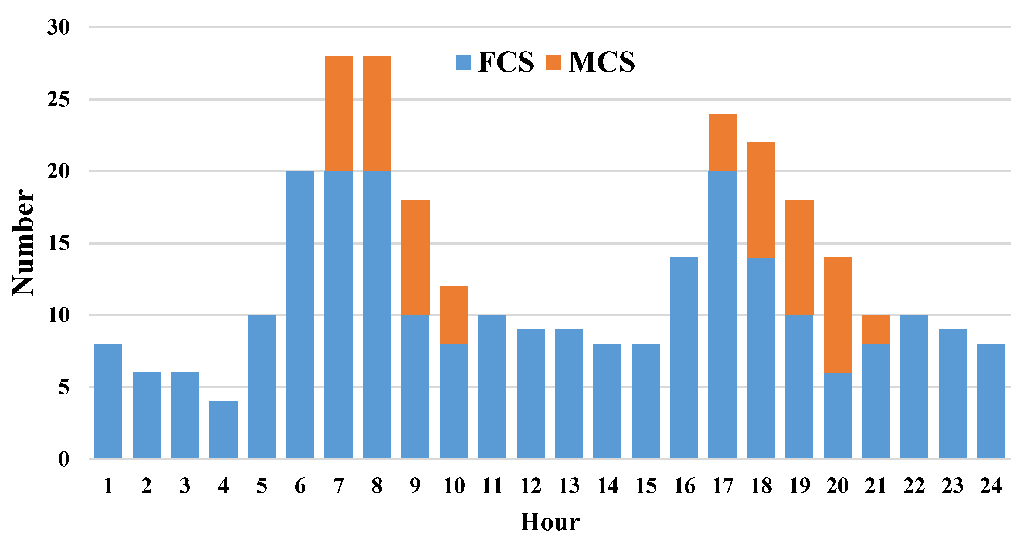
Figure 5. It is also assumed that renewable resources’ power production cost is zero owning to the network operator’s ownership. The hourly requests for the EV charging are as
Figure 6, each demanding 25 kWh of energy.
For the sake of simplicity and without loss of generality, it is assumed that both the fixed and mobile charging stations use fast chargers, which fully charge the EV batteries at one hour [
25]. In other words, each EV spends only one hour in the station under charging and with 25 kW of drawn power.
Due to the dependence of battery lifetime on the discharging power rate, employing a fast charging method may reduce battery lifetime. This study has ignored this effect to match the EVs charging time with the operation horizon time slices. On the other hand, using fast chargers will reduce the charging time the EV has to be spent in the station to fully charged.
The fixed charging station at bus 31 is capable of charging 20 vehicles per hour. The network is also equipped with a mobile charging station with 200 kW of power rating and 800 kWh of energy capacity. The MCS battery’s power rating can charge eight EVs per hour if enough stored energy is available. It is located at bus 1 with zero initial energy at the beginning of the time periods, and the charging and discharging efficiencies are both 0.95. It is also considered that, because of the space requirements for MCS and EVs parking for charging, the mobile charging station can be charged at buses 1, 3, 6, 12, 22, 25, and 31. On the contrary, it can only be discharged for EV charging when located at bus 31. In other words, the stored energy in the mobile battery is used only for EV charging. The transportation time between all candidate locations is considered to be one hour, and the consumed energy for each transport is equal to 2 kW per hour. The model is simulated for two cases, the case without MCS and the case with MCS. Then, the obtained results are analyzed and compared to evaluate the effectiveness of using the MCS.
The main results of the simulations are presented in
Table 1. It contains the total daily operation cost and the statistics related to the fixed charging station for both cases. In this regard, the hourly charging queue and consumed energy are calculated from Equations (24) and (12). The total daily charging queue and empty sockets are obtained by elaborating the corresponding hourly values over the day’s total hours. The number of FCS under charging EVs is calculated using Equation (22) or Equation (23), regarding the problem situation. In other words, the relation between the total number of charging requests and the available capacity of the MCS defines the number of under charging EVS in the FCS. Besides, the number of MCS empty sockets is equal to its charging sockets minus under charging EVs. Accordingly, the total daily operation cost is reduced by
$314, equivalent to about a 3.5% reduction due to using and optimizing the MCS. Besides daily operation cost reduction, the statistics related to EV charging are also improved. The total daily charging queue is reduced from 64 to only four, which shows about 94% improvement.
In addition, the total daily available empty sockets in the fixed charging station are increased by 58, meaning an 18.53% growth. This means that a significant part of the fixed charging station’s load is transferred to the mobile charging station due to the lower charging cost. In other words, the MCS not only causes a reduced charging cost but also diminishes the load on the fixed charging station result in a lesser charging queue. A total number of 58 EVs are transferred to the MCS in the whole day, resulting in reducing exactly the same amount of charging load on the fixed charging station. The last column of
Table 1 indicates the total energy consumed by the fixed charging station in both cases, along with the net and relative difference. As expected, the energy drawn from the grid is reduced by the amount of reduced charging station load, namely 18.53%.
Figure 7 depicts the number of under charging EVS at the MCS and FCS. It magnifies the impact of the MCS deployment on the peak charging demand reduction. MCS behavior is described in the following. The MCS has spent the first five hours of operation in bus 1. It was then transported to bus 31 at 6 o’clock and has been at this bus location from 7 A.M. to 10 P.M. Finally, the battery is transported again during hour 23 to be at the initial location at the last time period, namely hour 24 at bus 1. MCS battery hourly power and energy profile are shown in
Figure 8 and
Figure 9, respectively. Based on the results, the MCS has performed two charging-discharging cycles according to the two peaks of the EV charging demand. The first cycle is assigned to the first peak EV charging demand during 7–10 A.M.
To this end, the battery is charged during 1–5 A.M. As can be observed, the total charging energy in this period is equal to 844 kWh. Considering having a generic (non-ideal) battery and storing a net value of 800 kWh stored energy, a 0.95 charging efficiency is denoted by the results. Then, the stored energy is discharged for charging the EVs’ batteries during 7–10 A.M. For the second peak load on the fixed charging station, the MCS is charged from 11 A.M. to 3 P.M. to be able to discharge during 5–9 P.M. Another point is that the MCS battery is not entirely discharged at 10 P.M. and keeps a small amount. This energy, 2 kWh, is the amount that the MCS needs to relocate to the initial location due to its self-powered mechanism.
The hourly charging queue in the fixed charging station for both cases is depicted in
Figure 10. As can be observed, the fixed charging station experienced the highest charging queue during morning hours without employing the MCS, namely 7–9 A.M. In this period, at most, 16 EVs are in the charging queue. Besides, there is a lighter charging burden during evening hours between 5–9 P.M when the MCS is not used.
Using the MCS, the fixed charging station will have a very small load of the charging queue only at 7 A.M. and 8 A.M. More precisely, using the MCS and reducing the fixed charging station’s load, the queue of EVs for charging will be reduced to only three at 7 A.M. and two at 8 A.M., which is a negligible value.
Figure 11 presents hourly available empty sockets for charging in the fixed charging station for both simulation cases. Based on the results, the MCS helps reduce the charging queue during peak demand hours and increases the empty sockets by reducing the fixed charging station’s load at other times. This, in turn, will increase the station’s flexibility in accepting more EVs.
The hourly power drawn from the grid due to EV charging in the fixed station at bus 31 is depicted in
Figure 12. As can be observed, the fixed charging station energy demand has declined over two periods. The first one is related to the first peak EVs charging demand, from 8–11 A.M. The second period is related to the second and lower peak of the EVs’ charging load during 5–9 P.M. The fixed charging station energy demand pattern is entirely in accordance with the MCS behavior discussed previously. In other words, these two periods are in line with the MCS’ battery discharging periods presented in
Figure 8 or the stored energy depletion pattern in
Figure 9. The reduction in the energy demand of the fixed charging station will, in turn, impact other technical parameters of the network, which is described in the following.
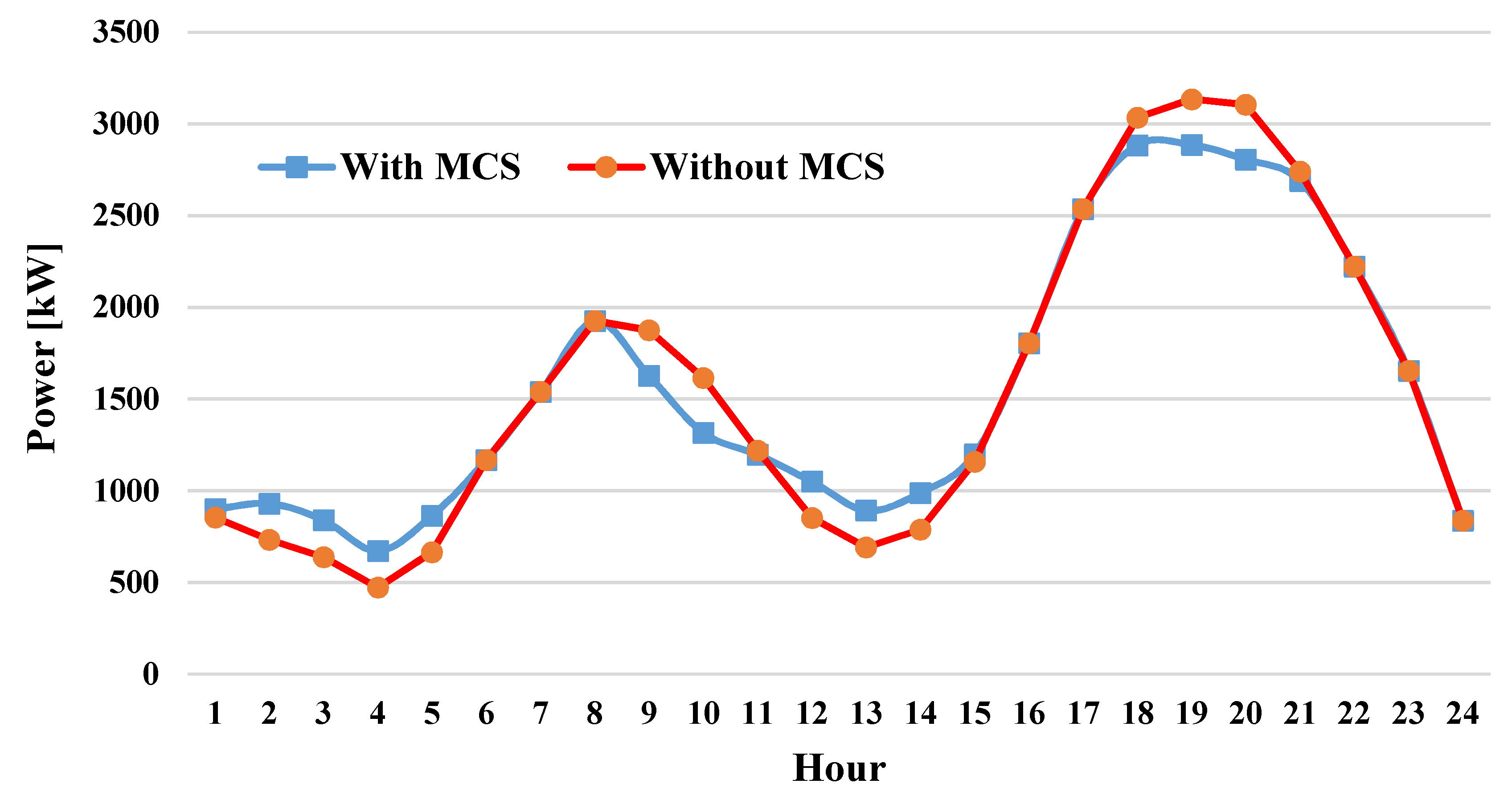
The hourly output power of the up-stream substation for the network without MCS and the network with MCS are shown in
Figure 13. Accordingly, the substation’s output power has experienced two cycles of the subsequent decrease and increase due to using the MCS. These increases and decreases are related to the charging and discharging of the MCS’ battery, respectively. In the first power decrease, the battery is charged during 1–5 A.M. Then, it is discharged for charging EVs at the first peak of charging demand. This, in turn, causes a decreasing charging load of the fixed charging stations, demanded power, and finally drawn power from the substation during 8–11 A.M. This increase and decrease power cycle are repeated in the subsequent time periods. Accordingly, the fixed charging station’s power demand at the peak period is reduced effectively employing the MCS. This peak shaving is performed by releasing the previously stored energy during hours 11–15 at the peak power demand during 6–10 P.M. As a result, the MCS’s energy arbitrage has reduced both the EV charging queue and electricity cost. However, it has also significantly reduced the peak load of the network. Reducing the network’s peak load, in turn, will reduce the voltage drop across the lines. This reduction will improve the network buses’ voltage during peak hours and bring the voltage range closer to one per-unit’s nominal value.
Figure 14 presents the voltage magnitude of the network buses at peak load hour, namely 8 P.M. It validates the positive impact of the MCS optimal operation on the buses’ voltage. As can be observed, the voltage of the network buses demonstrates an increase at two time periods. This increase in the buses’ voltage directly results from the charging load reduction of the fixed charging station and lower power flow in the network lines.
The sensitivity of the results with respect to the MCS’ battery specifications is performed, and results are provided in the following.
Table 2 presents the impact of changing the MCS’s battery’s power rating on the results. It contains the total daily operation cost, total daily EVs charged by the MCs, and the total daily queue of the EVs’ for charging in the fixed charging station. It should be noted that the charging sockets of the MCS are also changed concerning its battery’s power rating. In other words, considering the 25 kW charging power of each socket, the power rating is divided by this value to obtain the number of MCS charging sockets.
As can be observed, besides decreasing total daily operation cost, increasing MCS’s battery power rating will decrease the EV charging queue. The reduction in the charging queue is in line with the number of under charging EVs in the MCS. In other words, by increasing the power rating of the MCS’s battery, the charging queue of the EVs is decreased as a result of increased charging sockets in the MCS and consequently the number of charged EVs.
Table 3 shows the same results for the changes in the energy capacity of the MCS’s battery. The effect of changing the batteries’ energy capacity from 500 kWh to 1100 kWh on the results is also provided in
Table 3. As was expected, decreasing the energy capacity of the MCS’s battery will decrease obtained benefits. Strictly speaking, by reducing energy capacity from 1100 kWh to 500 kWh, the total daily operation cost will increase by
$153 per day. Also, the number of EVs in the charging queue will reach at most 24, which denotes a total daily number of 38 EVs charged in the MCs. It should be noted that, based on the obtained results, the impact of the power rating on the obtained benefits of using MCs is much more than the energy capacity.


