Article

Prediction Performance Analysis of Artificial Neural Network Model by Input Variable Combination for Residential Heating Loads

1
Department of Building and Plant Engineering, Hanbat National University, Daejeon 34158, Korea
2
Department of Architectural Engineering, Hanbat University, Daejeon 34158, Korea
3
Department of Architectural Engineering, Ulsan University, Ulsan 44610, Korea
*
Author to whom correspondence should be addressed.
Submission received: 21 December 2020 / Revised: 21 January 2021 / Accepted: 26 January 2021 / Published: 1 February 2021
(This article belongs to the Special Issue Data-Driven Energy-Cost Analysis of HVAC System for Buildings)

Abstract

:
In Korea apartment buildings, most energy is consumed as heating energy. In order to reduce heating energy in apartment buildings, it is required to reduce the amount of energy used in heating systems. Energy saving in heating systems can be achieved through operation and control based on efficient operation plans. The efficient operation plan of the heating system should be based on the predicted heating load. Thus, various methods have been developed for predicting heating loads. Recently, artificial intelligence techniques (e.g., ANN: artificial neural network) have been used to predict heating loads. The process for determination of input data variables is necessary to obtain the accuracy of predicted results using an ANN model. However, there is a lack of studies to evaluate the accuracy level of the predicted results caused by the selection and combination of input variables. There is a need to evaluate the performance of an ANN model for prediction of residential heating loads. Therefore, the purpose of this study is, for a residential building, to evaluate the accuracy levels of predicted heating loads using an ANN model with various combinations of input variables. To achieve the study purpose, each case was classified according to the combination of the input variables and the prediction results were analyzed. Through this, the worst, mean, and best were selected according to the predicted performance. In addition, an actual case was selected consisting of variables that can be measured in an actual building. The derived cv(RMSE) of each case resulted in a percentage value of 38.2% for the worst, 7.3% for the mean, 3.0% for the best, and 5.4% for the actual. The largest difference between the best and worst resulted in 33.2%, and thus the precision of the predicted heating loads was highly affected by the selection and combination of the input variables used for the ANN model.

1. Introduction

1.1. Background and Purpose

In 2018, the Intergovernmental Panel on Climate Change (IPCC) recommended stabilizing the increase of the Earth’s surface temperature to within 1.5 °C compared to the period before industrialization [1]. In addition, the achievement of Net Zero, which minimizes anthropogenic carbon emission by 2050, is becoming a common international goal. To accommodate and accomplish these international goals and perception change, it is essential to reduce greenhouse gas emissions in the energy sector, which accounts for 86.8% of the total national greenhouse gas emissions in Korea [2]. Accordingly, there have been continued nationwide efforts to save energy in the fields of industry, power generation, buildings, and transportation. In particular, the building sector continues to strengthen related regulations in an attempt to save energy [3].
Energy consumption in buildings in Korea stems mostly from energy use in apartment buildings, hospitals, schools, and commercial buildings (see Figure 1) [4]. Among them, the energy consumption of apartments is about 17.0%, accounting for the largest percentage. Therefore, energy saving and efficient energy usage in relation to apartment housings will have a significant influence on energy maintenance throughout the country. In particular, about 67.1% of the energy consumed in apartment housings in Korea is used for heating, so it is required to focus on heating energy reduction [5]. Therefore, the use of high-efficiency systems that can save energy (district heating systems, geothermal heat pumps, high-efficiency boilers, etc.) is increasing. However, the performance of these heating systems can be maximized only when optimal system operation and control are involved. In general, to operate the systems at an appropriate and optimal level, it is essential to predict and evaluate the heating load that a heating system must handle. If a demand for the heating loads is identified in advance and an optimal system operation for the heating loads is planned, it is possible to prevent overheating and to save energy. Furthermore, the system operation plan based on the identified heating loads may enhance thermal satisfaction in indoor spaces. Therefore, it is necessary for the technology on predicting heating loads to minimize over/under heating usages and to maintain a comfortable indoor space environment.
To achieve optimal control of the heating system based on the predicted heating loads, the temporal scale of the predicted heating load is important If the temporal scale of the heating loads predictive model is the same as the control time (timestep), it is possible to efficiently control according to variation of the heating demand.
In general, the typical heating load evaluation methods include the equation-based load calculation for building facades, simulation programs (EnergyPlus [6], TRANSYS [7], DOE-2 [8], etc.), regression models, and artificial intelligence techniques. Among them, the equation-based load calculation for building façades and simulation programs require various and detailed input parameters for each structure of a building. This significantly affects the accuracy and reliability of the heating load calculation result. However, when using a regression model and artificial neural network (ANN), relatively simple input variables are required. In particular, the ANN model has a high computational speed and excellent prediction performance for energy prediction regarding existing buildings [9]. The prediction performance of the ANN model depends on data type and quality. Therefore, data preprocessing and selection of input and output variables are very important. When selecting input variables and output variables, how input variables affect output variables should be analyzed in advance. Therefore, this study analyzed and evaluated how the setting of input variables affects the heating load prediction results when predicting the heating load of an apartment housing using the ANN model.

1.2. Literature Review

To determine the input variables used for an ANN model, this study conducted a literature review associated with the predicted heating loads, especially using artificial intelligence techniques. It should be noted that this study did not include previous literatures based on an equation and/or simulation program since they have fixed input variables used for the prediction. This study categorized the determined input variables by the physical thermal relationship. That is, heating loads are generally influenced by the outdoor/indoor environment, building materials, mechanical heating system, and others. The determined input variables were divided into four categories: weather, construction, zone, and system. The summary of the conducted literature review is given in Table 1.
Among the reviewed studies, 16 cases used artificial intelligence (AI) techniques and 8 cases used regression models (Reg). In particular, 13 cases used artificial intelligence techniques and 6 cases used regression models over the last 7 years (2014–2020). However, in five out of the six cases that used a regression model, artificial intelligence techniques were also employed, so only one study used a regression model alone. Based on the literature review, it was identified that the majority of the prediction methods for the heating load were the AI techniques.
Weather data was selected to reflect the effect of outdoor thermal conditions, regional characteristics, etc. of buildings on heating loads. Weather data were classified into outdoor air temperature (OAT), solar radiation (Solar), relative humidity (RH), wind speed (V), and other items. The outdoor air temperature was used as an input variable in 12 studies. This was the most frequently used item among the input variables used to predict a heating load. Solar radiation was used as an input variable in eight cases, relative humidity in three cases, and wind speed in five studies.
Construction data were selected to reflect the effect of building thermal conditions, geographic characteristics, etc. of buildings on heating loads. Construction data were classified into heat permeability (U-value), building area (A: Area), window-to-wall ratio (WWR), and building orientation (BO). Heat permeability was used as an input variable in two studies, building area in nine studies, window-to-wall ratio in two studies, and building orientation in seven studies.
Zone data were selected to reflect heat gain and the operation status of the building. Zone data, i.e., zone mean air temperature (ZMT), schedule (Sch), and heating load (HL), were used as input variables in two studies. Zone data were used to reflect the characteristics of residents’ heating usage.
System data were selected to reflect heating loads according to facility operation. System data were classified into supply water temperature (SWT), mass flow rate ( m ˙ ), and return water temperature (RWT) and were used as input variables in three studies.
This study selected input variables based on prior studies, evaluated the prediction performance based on the combination of each input variable, and defined the combination of input variables. For this, each variable of weather, construction, zone, and system data was selected, where a variable that is frequently used in each item was used as an input variable. OAT and solar were selected for the weather data and A and BO were selected for the construction data. These four variables were the second most used variables in prior studies. Regarding zone data and system data, all variables were considered because all the variables were used in the same number of prior studies. Therefore, ZMT, Sch, and HL were selected for the zone data and SWT, RWT, and m were selected for the system data.
In addition, when reviewing prior studies, studies, except for [14] and [22], predicted the current heating load based on the current timestep data. Those two studies, i.e., [14] and [22], used past data based on the past heating load history. However, variables other than the past heating load history were used based on the current timestep data. Therefore, the prior studies referenced in this study cannot predict the current heating load if the current timestep data cannot be obtained. In general, it is required to understand a heating load in advance to devise an efficient operation plan of a heating system. For this, it is necessary to predict the current heating load based on the past timestep data. Therefore, in this study, the ANN model that predicts a heating load based on the past data was used to analyze the effect of input variables and a model that predicts a heating load based on the past data was developed.

2. Methodology

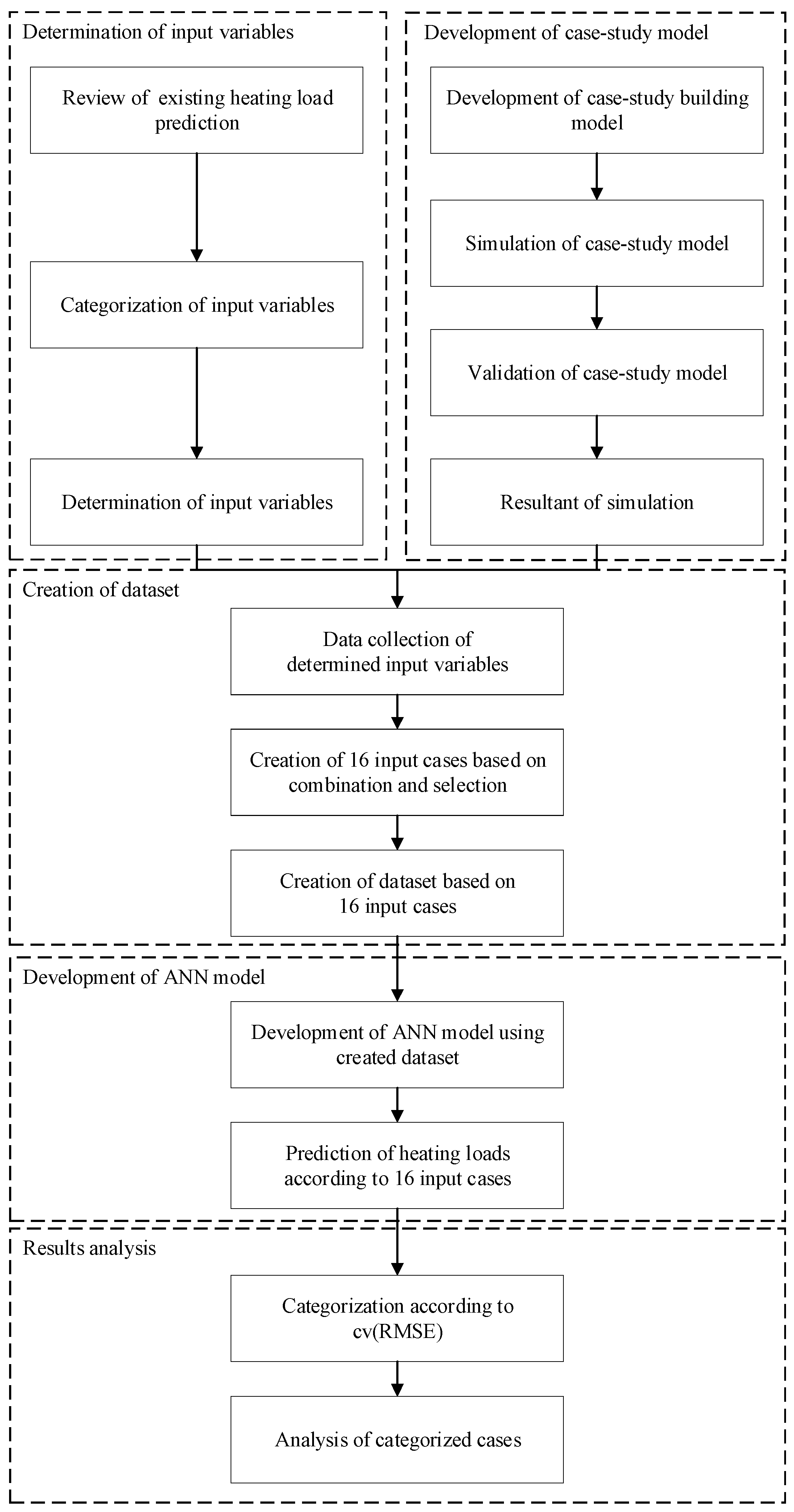
2.1. Overall Study Process

This study evaluated the influence of input variables on the ANN model when predicting a heating load and analyzed the predicted heating load. Figure 2 shows the overall flowchart of this research.
To configure the input variables of the ANN model, previous studies on building load prediction were reviewed (see Section 1.2). Input variables were selected based on the reviewed previous studies.
A case-study simulation model that can simulate the thermal behavior of an actual building was developed to produce a dataset of the ANN model. The case-study model was developed based on an apartment housing located in Daejeon, Korea. EnergyPlus was used to develop the model. The case-study model was verified by comparing its result with the heating load value of an actual apartment building. Data of the selected input variables and the heating load were extracted through the case-study model and a dataset was developed based on the results. To develop the ANN model, this study utilized the Neural Network toolbox included in MATLAB [32].
The input variables selected to configure the input variables of the ANN model were classified into essential variables and optional variables. Each case was classified according to the combination of optional variables. Weather data that can be easily measured and which have been widely used in prior studies were used as essential variables. The ANN model predicted a heating load using the input variables of each case. The error rate was analyzed based on the predicted data. The prediction results were analyzed by selecting three cases (worst, mean, and best) based on the calculated error rate. In addition, the prediction results were analyzed by selecting an actual case consisting of input variables that can be measured in an actual apartment building.

2.2. Case-Study Simulation Modeling

This study developed a case-study model that can realize the thermal behavior of an actual apartment building to produce a dataset of the ANN model. For this objective, this study developed a simulation model based on apartment A in Daejeon, Korea. The heating system of apartment A uses district heating as a heat source. The zone configuration was classified according to the outer wall insulation characteristics of the location of each household in the case-study building, where A and F were sidewall households, B was the middle household, and C and E were households facing the non-heating spaces and middle households. The case-study model used Daejeon weather data for the simulation obtained from IWEC2 (International Weather Files for Energy Calculation 2.0) weather files [33]. Table 2 presents the monthly outdoor air temperatures during the heating period, including the minimum, maximum, and average values of the Daejeon weather data. The lowest average temperature, −1.2 °C, was observed in January, and this month had a minimum of −18.8 °C and a maximum of 10.3 °C.
EnergyPlus was used to develop a case-study model that reflects the characteristics of apartment A. The produced model consists of the ground floor, middle floor, and top floor to reflect the load characteristics of low, middle, and high floors of an apartment housing by varying the thermal boundary conditions of the floors and ceilings of each three floors. The remaining simulation conditions were produced based on apartment A. Table 3 shows the simulation parameters. Figure 3 shows the zone configuration of the actual apartment building and the shape of the case-study model.

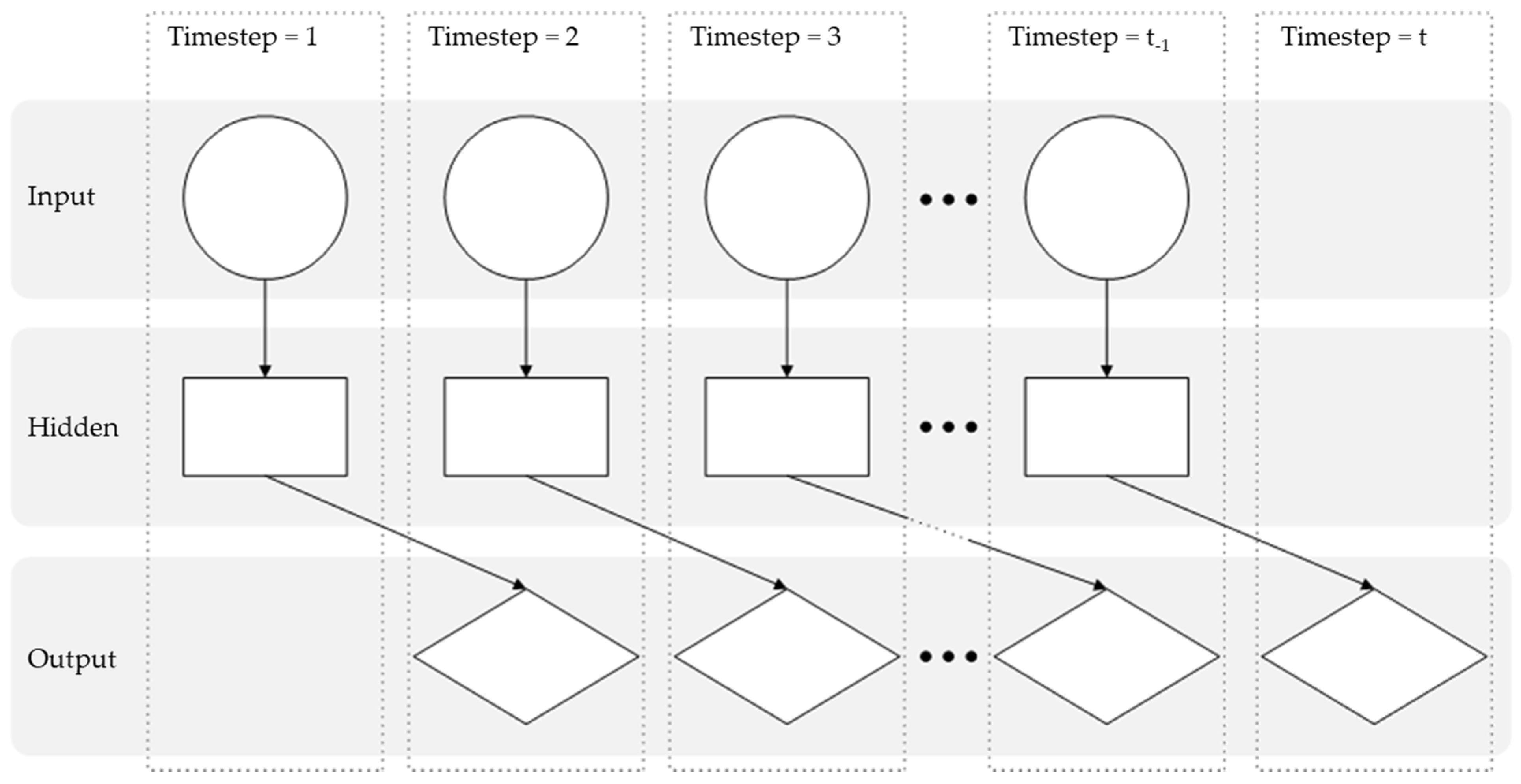
2.3. Development of Artificial Neural Network Model for Heating Load Prediction

In this study, a dataset was created to develop the ANN-based heating load prediction model. The dataset used data from 13 January to 19 January. The resultant data extracted from EnergyPlus simulation for the case-study model were used for the dataset to develop the ANN model.
In addition, since the ANN model predicted the future heating loads using current input data, the datasets were arranged. The temporal scale of the predicted heating loads was set as the next timestep (10 min). Figure 4 is the timestep of the input values and target values of the ANN model designed in this study.
In this study, the ANN model was developed to determine input variables. Table 4 shows the information of the ANN model. The ANN model was developed using MATLAB’s Neural Network toolbox. The number of hidden layers (NHLs) was set to one layer. The number of hidden neurons (NHNs) value was calculated using Equation (1) [34], where N is the sum of the input and output variables. Therefore, in this study, NHN was set to 23 by using all input and output variables. The learning rate (LR) and momentum constant (MC) were set to 0.3, epochs to 1000, and goals to 0.001. In ANN, arbitrary values are used for variables other than NHN because there are no defined criteria when setting structural parameters and parameters.
N u m b e r   o f   h i d d e n   n e u r o n s   =   2 N + 1
The input variables of the ANN model for heating load prediction were selected through prediction performance evaluation depending on the combination of each variable of weather data, construction data, zone data, and system data. The cv(RMSE) (coefficient of variation of the root mean square error) was used for prediction performance evaluation. The cv(RMSE) is a relative error obtained by dividing the root mean square error (RMSE), which is the difference between the predicted value and the measured value, by arithmetic means. Equations (2) and (3) are the equations to calculate RMSE and cv(RMSE):
R M S E   =     ( S M ) 2 P r e i o d N
c v ( R M S E )   =   R M S E A P r e i o d   [ % ]
Regarding weather data, the outdoor air temperature (OAT), diffuse horizontal irradiance (DHI), direct normal irradiance (DNI), and ratio of outdoor air temperature (ROAT) were selected because they were the most frequently used variables in prior studies. The ratio of outdoor air temperature, i.e., a variable proposed in this study to improve prediction performance, is the change rate of outdoor air temperature during 3 timesteps (i.e., 30 min). Equation (4) is the equation to calculate the ratio of outdoor air temperature, where t is the current timestep and t 3 is the data 3 timesteps (i.e., 30 min) before:
R O A T   =   O A T t     O A T t 3 3
Based on the prior 12 studies that predicted a heating load using construction data, A and BO, which were used most frequently, were selected as input variables. However, most of the studies referenced in this study were conducted to predict a heating load depending on the change of the variable value of a building structure. Therefore, in this study, there is no change with the variable of a building structure, so the selected construction data were not used as an input data.
The zone data of prior studies were reviewed in order to select a zone data for this study. As a result, the prior studies predicted a heating load using the zone mean air temperature, previous heating load, and schedule. Since measured heating load data could not be obtained for the target building, the previous heating load was excluded for the selected input variables in this study. In addition, the building operation schedule was also excluded for the input variable selection. The reason was that the developed case-study simulation model was validated against the certified load data obtained from the target building using a constant schedule value (i.e., always on). Accordingly, only the zone mean air temperature was used as an input variable among the selected zone data variables.
In the case-study simulation, district heating was used as a heat source. In general, a heating system using district heating as a heat source that consists of a primary side loop that supplies water from the heat source production site to the machine room of an apartment housing and a secondary side loop that sends water from the machine room of the apartment housing to households (Figure 5). Since this study was conducted for apartment buildings, the system data of the secondary side loop connected to an apartment housing was used. Accordingly, the supply water temperature, mass flow rate, and return water temperature were used as system data.
To configure input variables, each input variable of weather, zone, and system data was selected. For the combination of selected input variables, they were classified into essential and optional variables, where the weather data, i.e., a variable that can be easily measured and is widely used in prior studies, was selected as an essential variable. The zone and system data were selected as optional variables. The input variables were defined by evaluating the prediction performance depending on the combination of selected optional variables.
Table 5 shows the input parameters of the ANN model. Table 5 presents value ranges for the determined input variables based on the EnergyPlus simulation results, and these ranges were considered as the environment and system operation values used for the ANN model. The value range of each selected input variable is different. In general, if the value range of an input variable of the ANN model is different, the predicted value is dependent on the variable with a larger value range [35]. Therefore, this study used a normalization technique to adjust the value range of an input variable to a common range. For this, Equation (5) was used, and it employs the min-max normalization technique, where x is an original value, x_min is a minimum value of the original value, and x_max is a maximum value of the original value.
x N o m a l i z e d =   x     x m i n x m a x     x m i n

3. Results

3.1. Validation of the Case-Study Simulation Model

This section explains the validation of the EnergyPlus case-study model developed for the actual apartment buildings. To verify the case-study model, it was compared to the annual heating loads of an actual building. The mean absolute error (MAE) and mean absolute percentage error (MAPE) were used as indices for evaluation. The case-study model was compared to the annual heating loads of three floor types of the apartment building. The results are shown in Table 6. The MAE value for each floor type was about 2.4 for 39A type, about 0.7 for 39C type, and about 30.6 for 46A type and the MAE value for all floors was about 5329. The MAPE value was about 1% for 39A type, about 0.2% for 39C type, and about 14% for 46A type, and the overall average MAPE value of all floors was about 7%.

3.2. Heating Load Prediction using the Developed Artificial Neural Network Model for

Input variables were classified into essential variables and optional variables and they were classified into each case according to the combination of optional variables where the weather data was set as an essential variable and the zone data and system data were set as optional variables. Using the prediction performance results of each case, the worst case (the lowest prediction performance), the mean case (the middle), and the best case (the highest prediction performance) were selected. In addition, the combination of variables that can be measured in an actual apartment building was selected as an actual case. The combination of input variables and prediction performance results of each case are summarized in Table 7. When evaluating the prediction performance depending on optional variables, the prediction performance of case 1 was the lowest with a cv(RMSE) value of about 38.2%. This was selected as the worst case and the input variables were OAT, DHI, DNI, and ROAT. The prediction performance of case 2 was about 7.3% based on cv(RMSE) and it was selected as the mean case, which is the middle level among all cases. Its input variables were OAT, DHI, DNI, ROAT, and ZMT. The best case was case 16, where the cv(RMSE) value was about 3.0%. The input variables of the best case were OAT, DHI, DNI, ROAT, ZMT, SWT m ˙ , and RWT. The actual case is a case using variables that can be measured in an actual apartment building. The actual apartment building referenced in this study does not have a flow meter installed in its machine room due to cost issues. Therefore, input variables that can be measured were selected as OAT, DHI, DNI, ROAT, ZMT, SWT, and RWT (i.e., case 13). The prediction accuracy was about 5.4% based on cv(RMSE). In this study, four cases were selected depending on the prediction performance and measurable variables. As a result, case 1, 2, 16, and 13 were selected as the worst, mean, best, and actual case, respectively.

4. Analysis and Discussion

The heating load prediction results of the four selected cases were analyzed. Figure 6 shows the comparison results between EnergyPlus and the predicted loads using the ANN model of the worst, mean, best, and actual case in order from (a) to (d), where the X-axis represents the EnergyPlus result data and the Y-axis represents the predicted load using the ANN model. In addition, a trend line and R2 are displayed on each graph, where R2 is a value between 0 and 1 and the X-axis value and Y-axis value are the same when R2 is 1. R2 of each case was 0.5983 for the worst case, 0.9854 for the mean case, 0.9976 for the best case, and 0.9921 for the actual case. Therefore, the predicted data of the mean, best, and actual cases were similar to the trend of the reference data value. However, in the worst case, the trend of the reference data was not reflected well in the predicted data.
Figure 7 shows the comparison results between the predicted data and referenced data of each case over time, where SWT is 52 °C and m ˙ is 0.55 kg/s. These are the predicted results on 13 January. The prediction results of the worst case were inaccurate in general. The predicted data changes according to the large change trend of the referenced data, but the value difference was inaccurate at an average of about 2610 W. In addition, it did not reflect the fluctuation of a load that changes in a short period of time. Therefore, it is unlikely that the prediction results of the worst case will be reliable.
The prediction result of the mean case was similar to that of the referenced data. However, when a load changes within a short period of time, such as from 02:40 to 03:10, from 03:30 to 04:10, or from 06:30 to 07:10, the prediction accuracy deteriorated. The value difference between the referenced data and predicted data was about 516 W on average.
The best case gave a very accurate prediction result. The prediction results were excellent even with the changing trend of the referenced data and a load changing within a short period of time. The value difference between the referenced data and predicted data was about 13 W on average.
The prediction result of the actual case also reflected the change trend of the referenced data. However, the prediction accuracy declined when a load changed within a short period of time just like the mean case.
Therefore, when predicting a daily load, it is likely that the prediction accuracy can be secured for the cases other than the worst case. However, it is likely that accurate prediction will be possible only in the best case when predicting a heating load for a short period of time.

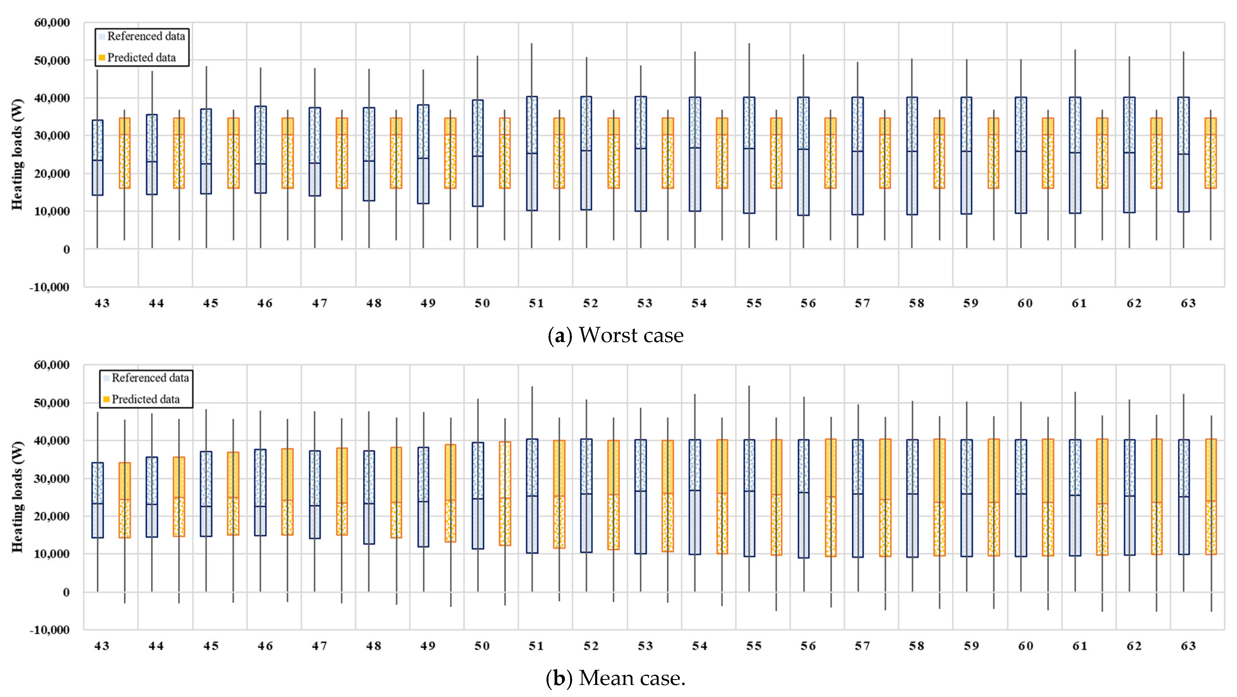
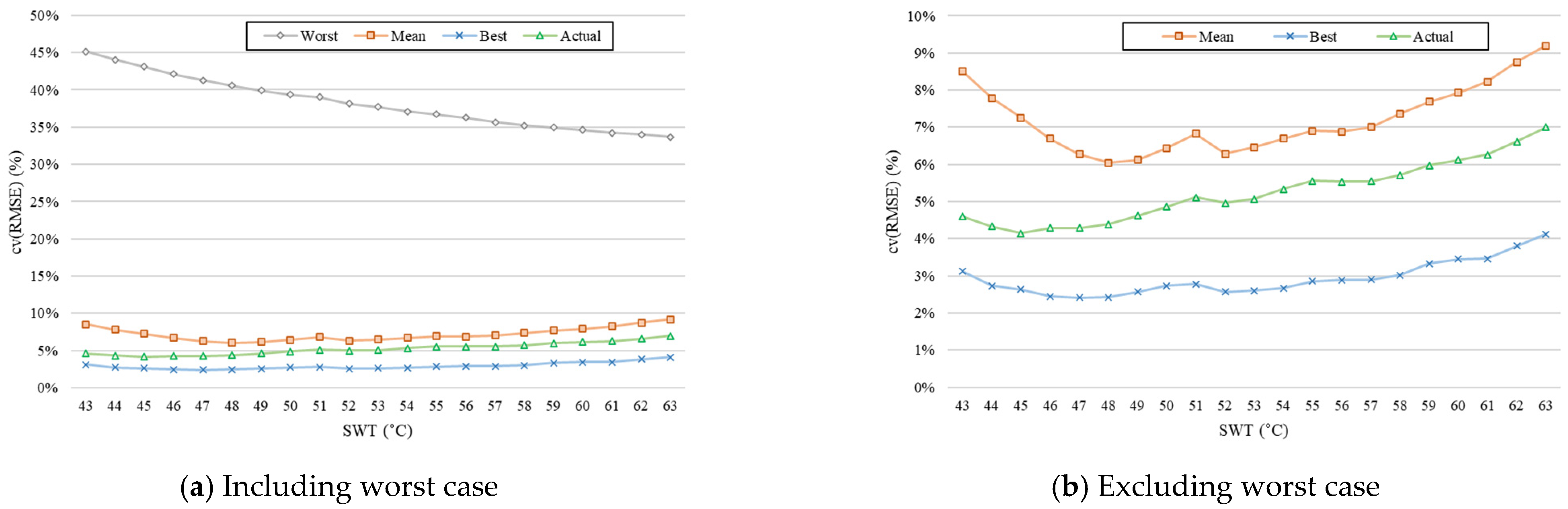
4.1. Analysis of the Prediction Results According to the Supply Water Temperature

The ANN model developed in this study was designed to predict a heating load when the SWT was controlled between 43 °C and 63 °C. Therefore, the heating prediction value and referenced data of each case were analyzed according to SWT using a box plot (see Figure 8). As a result, the range of the predicted heating load value in the worst case was similar to the referenced data based on the data between 25% and 75% in the range of 43 to 45 °C and the value was different from the reference data in other temperature ranges. However, the prediction accuracy was the lowest based on cv(RMSE) when the SWT was 43 °C. In the mean case, the prediction performance was the best at 48 °C and it was the lowest at 63 °C. In the best case, the prediction performance was the best at 47 °C and the cv(RMSE) was about 2.41%. The SWT with the lowest prediction performance in the best case was 63 °C. In the actual case, the prediction performance was the best with a cv(RMSE) value of about 4.15% at 45 °C. The prediction accuracy was the lowest at 63 °C in the actual case.
Figure 9 is the result of cv(RMSE) analysis by temperature of each case. In the worst case, cv(RMSE) decreased as SWT increased. In the mean case and best case, cv(RMSE) decreased as SWT increased from 43 to 48 °C. However, when the temperature increased from 48 to 63 °C, cv(RMSE) decreased. In the actual case, when SWT increased, cv(RMSE) decreased to 45 °C, and cv(RMSE) increased as the temperature increased in other sections.
From the analysis results, all cases except the worst case showed an excellent prediction performance in general and the prediction accuracy was lowest at 63 °C. On the other hand, the worst case showed the best prediction performance at 63 °C.
When predicting a heating load according to SWT, cv(RMSE) for each SWT in the mean case where SWT was not used as an input variable was a maximum of 9.20%, a minimum of 6.04%, and an average of 7.21%. This means that load fluctuation according to SWT change is indirectly reflected. Therefore, it is likely that selecting ZMT as an input variable will help improve the prediction performance if it is difficult to obtain SWT data.

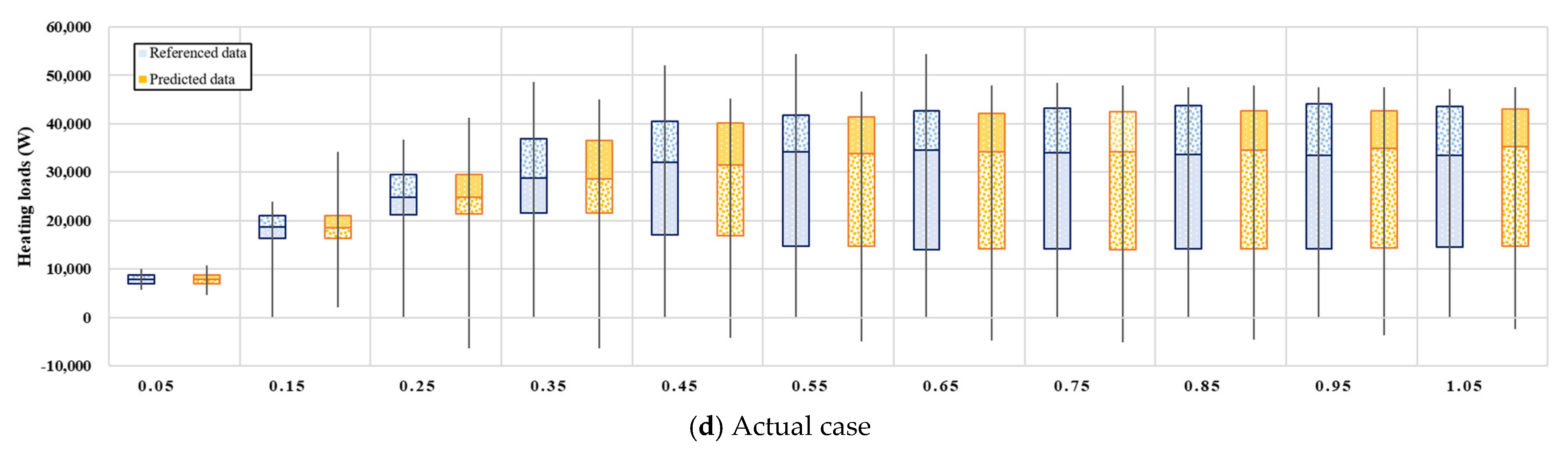
4.2. Analysis of the Prediction Results According to the Heating Mass Flow Rate

Figure 10 is a box plot of the heating load distribution predicted at intervals of 0.1 kg/s for the mass flow rate ranging from 0.05 to 1.05 kg/s. The worst case did not respond to the change in the flow rate and the change of the predicted heating load was insignificant when the flow rate changed from 0.05 to 1.05 kg/s. Here, it was impossible to predict the heating load because the cv(RMSE) was about 256.2% when the flow rate was 0.05 kg/s. In the mean case, the prediction accuracy was the lowest with a cv(RMSE) value of about 8.7% at 0.35 kg/s and the prediction accuracy was the highest with cv(RMSE) of 3.1% at 0.15 kg/s. The cv(RMSE) for each flow rate in the best case was a minimum of 1.7% to a maximum of 3.7%. The prediction accuracy of the actual case was from a minimum of 3.7% to a maximum of 5.8% based on cv(RMSE), the prediction accuracy regarding which was about 2% lower than the best case. In addition, the minimum cv(RMSE) was 0.6% higher than the mean case but about 3% lower than the maximum value.
Figure 11 shows the cv(RMSE) analysis results according to the mass flow rate of each case. From the cv(RMSE) analysis, the heating load prediction was very inaccurate when m ˙ was less than 0.25 kg/s in the worst case. However, in other cases, the cv(RMSE) was a minimum of 22.7% and a maximum of about 25.6%, enabling accurate prediction compared to the prediction result according to SWT. Therefore, it is likely that it is impossible to predict if m ˙ is less than 0.25 kg/s when predicting a heating load using only weather data. The mean cv(RMSE) of the mean case was about 6.7%, which is about 1.6% higher than that of the actual case, but it was about 0.6% lower than the actual case when m ˙ is 0.15 kg/s. The average cv(RMSE) for each mass flow rate in the best case and actual case was about 2.8% and 5.1%, respectively.
Therefore, the average cv(RMSE) of each flow rate in the mean case and actual case without m ˙ as an input variable was about 6.7% and 5.1%, respectively. Therefore, it is likely that ZMT, SWT, and RWT can indirectly reflect the effect of m ˙ on a heating load. However, in the actual case, a heating load according to m ˙ was analyzed based on the prediction result when both SWT and RWT were used simultaneously. Therefore, it is necessary to analyze the heating load according to m ˙ by using a case (refer to cases 6 and 8) when either SWT or RWT is used as an input variable separately.

5. Summary and Conclusions

As there is an increasing demand for accurate heating load prediction, there have been continued research initiatives conducted with regard to accurate heating load prediction. In particular, there are an increased number of studies using an ANN model. To obtain proper predictive performance for ANN model applications, the process for the determination of input variables is critical. However, there is a lack of studies evaluating the resultant predictive performance according to the selection and combination of input variables. Therefore, this study aimed mainly to evaluate the precision of the heating loads predicted from an ANN model by various combinations of residential input variables. The input variables were classified into essential variables and optional variables and prediction performance was evaluated based on the combination of optional variables. Based on the prediction performance analysis results, the worst, mean, and best cases were selected and an actual case consisting of measurable data was selected. The prediction results of each selected case were analyzed. Based on the analysis results, the results of this study are as follows.
  • This study developed a case-study model to create the dataset of the ANN model. The case-study model was developed based on an actual apartment building. To verify the case-study model, it was compared with the annual heating loads of an actual apartment building. As a result, the MAPE was about 7%.
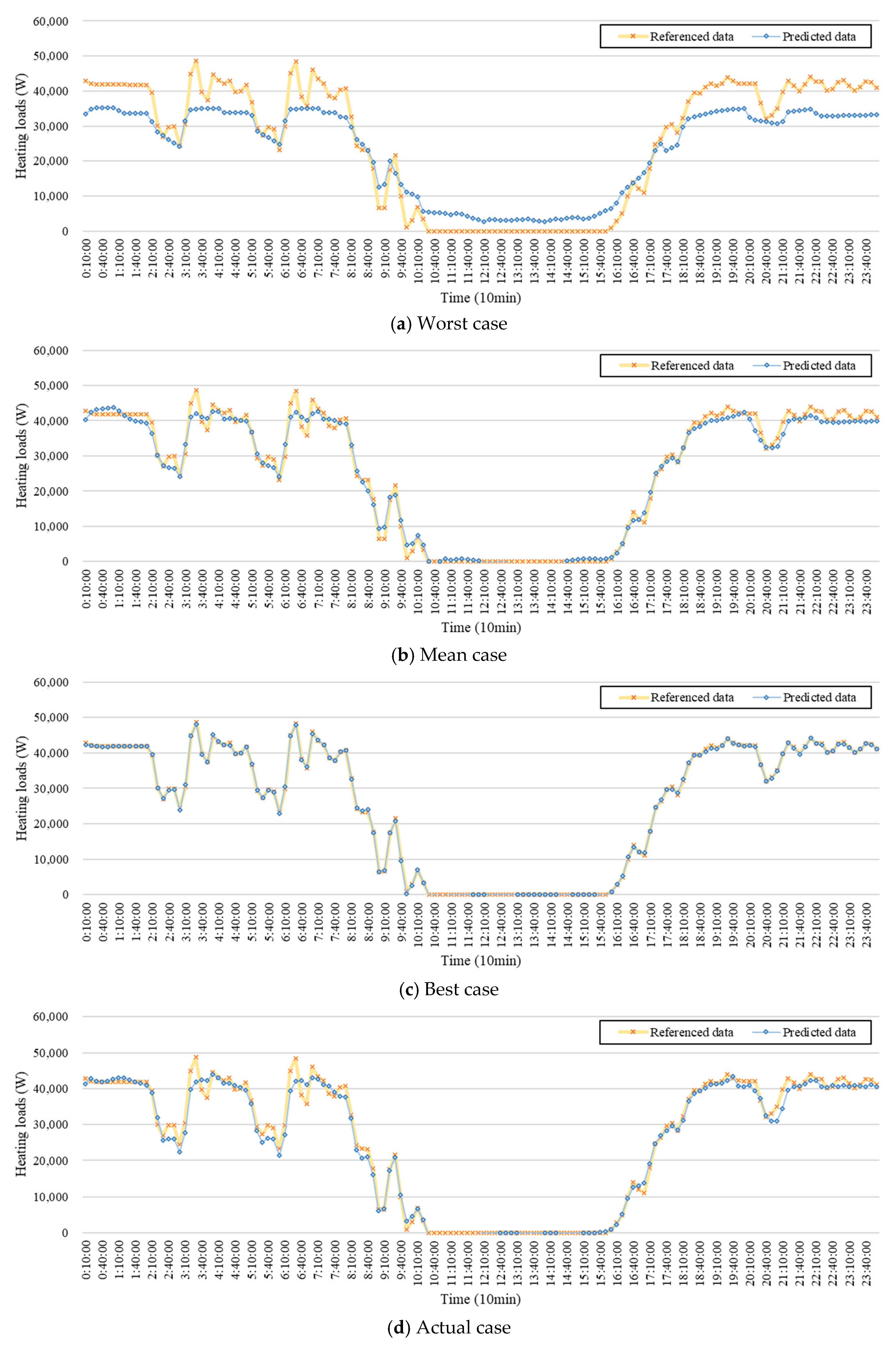
  • Various inputs were selected based on the prior studies. The selected input variables were classified into essential variables and optional variables and a total of 16 cases were created according to the combination of optional variables. The heating loads were predicted according to the combination of input variables of each case. The prediction accuracy of a predicted heating load was analyzed using cv(RMSE). The worst, mean, and best cases were selected based on the prediction performance, and an actual case consisting of measurable input variables in an actual apartment building was selected.
  • The prediction performance of each selected case was analyzed according to the supply water temperature and mass flow rate. In the worst case, it was impossible to predict the heating loads in general. In the mean case, the load fluctuation according to the influence of the supply water temperature and mass flow rate, which were not used as input variables, was reflected in the prediction results. Accordingly, it is likely that ZMT, i.e., the input variable of the mean case, can indirectly reflect the effect of SWT and m ˙ on the heating loads. The best case predicted the heating loads using all input variables, so its prediction performance was the best. In the actual case, it was possible to predict the heating loads according to the mass flow rate change, which was not used as an input variable. Therefore, ZMT may contribute to an improvement of the prediction performance if it is difficult to obtain SWT and m ˙ data.
This study predicted a heating load using the ANN model based on simulation data and evaluated the influence of input variables. The maximum and minimum differences between the best and worst cases were observed in 33.2% and 1.1%, respectively. Therefore, combinations of the selected input variables led to a significant impact on the heating load prediction performance. It can be concluded that the determination process for appropriate input variables should be accomplished when using an ANN model to predict residential heating loads. However, it should be noted that the evaluated results conducted in this study were based on simulation data driven by the EnergyPlus program. To solidify these results, therefore, additional study using an ANN model with actual measured data is recommended.

Author Contributions

All authors contributed equally. Conceptualization, C.L., D.E.J., S.L.D.; methodology, C.L., S.L.D.; formal analysis, C.L., D.E.J., S.L.D.; data curation, C.L., D.E.J., S.L.D.; writing—original draft preparation, C.L., S.L.D.; writing—review and editing, S.L.D., D.L., K. H. K.; visualization, C.L., D.E.J., D.L., K.H.K., S.L.D.; supervision, S.L.D. All authors have read and agreed to the published version of the manuscript.

Funding

This work was supported by the Korea Institute of Energy Technology Evaluation and Planning (KETEP) and the Ministry of Trade, Industry and Energy (MOTIE) of the Republic of Korea (No. 20204030200080). This research was also supported by the research fund of Hanbat National University in 2019.

Institutional Review Board Statement

Not applicable.

Informed Consent Statement

Not applicable.

Data Availability Statement

Not applicable.

Conflicts of Interest

The authors declare no conflict of interest.

References

  1. Intergovernmental Panel on Climate Change. Global Warming of 1.5 °C, Summary for Policymakers; IPCC: Geneva, Switzerland, 2018.
  2. Ministry of Environment (ME). National Greenhouse Gas Inventory Report of Korea; Greenhouse Gas Inventory and Research Center (GIR): Seoul, Korea, 2019.
  3. Ministry of Land Infrastructure and Transport. Green Buildings Construction Support Act; Act No. 15728; MOLIT: Sejong, Korea, 2008. Available online: https://elaw.klri.re.kr/kor_service/lawView.do?hseq=50008&lang=ENG (accessed on 10 June 2020).
  4. Ministry of Trade, Industry and Energy. End-Use Energy Statistics; MOTIE: Sejong, Korea, 2019.
  5. Korea Appraisal Board. Residential Building Energy Use; KAB: Daegu, Korea, 2018. [Google Scholar]
  6. The U.S. Department of Energy. EnergyPlus; version 8.5; DOE: Washington, DC, USA, 2016.
  7. University of Wisconsin-Madison. A Transient System Simulation Program Developed from Solar Energy Laboratory, TRANSYS; University of Wisconsin-Madison: Madison, WI, USA, 1990. [Google Scholar]
  8. The U.S Department of Energy. DOE-2 Building Energy Use and Cost Analysis Tool: DOE-2.1e; James J. Hirsch (JJH): Santa Rosa Valley, CA, USA, 2017.
  9. Song, S.M.; Oh, S.H.; Park, H.S. A Study on the Design Technique for the Building Energy Efficiency Rating Improvement of the Apartments; KIAEBS: Seoul, Korea, 2011; pp. 197–206. [Google Scholar]
  10. Kalogirou, S.; Neocleous, C.; Schizas, C. Building Heating Load Estimation Using Artificial Neural Networks. 1997. Available online: https://citeseerx.ist.psu.edu/viewdoc/download?doi=10.1.1.130.7125&rep=rep1&type=pdf (accessed on 30 January 2021).
  11. Kalogirou, S.; Florides, G.; Neocleous, C.; Schizas, C. Estimation of daily heating and cooling loads using artificial neural networks. In Proceedings of the 2001 World Congress, Naples, Italy, 15–18 September 2001. [Google Scholar]
  12. Linda, P.; Stang, J.; Ulseth, R. Load prediction method for heat and electricity demand in buildings for the purpose of planning for mixed energy distribution systems. Energy Build. 2008, 40, 1124–1134. [Google Scholar]
  13. Tsanas, A.; Xifara, A. Accurate quantitative estimation of energy performance of residential buildings using statistical machine learning tools. Energy Build. 2012, 49, 560–567. [Google Scholar] [CrossRef]
  14. Yun, K.; Luck, R.; Mago, P.J.; Cho, H. Building hourly thermal load prediction using an indexed ARX model. Energy Build. 2012, 54, 225–233. [Google Scholar] [CrossRef]
  15. Turhan, C.; Kazanasmaz, T.; Uygun, I.E.; Ekmen, K.E.; Akkurt, G.G. Comparative study of a building energy performance software (KEP-IYTE-ESS) and ANN-based building heat load estimation. Energy Build. 2014, 85, 115–125. [Google Scholar] [CrossRef] [Green Version]
  16. Chou, J.S.; Bui, D.K. Modeling heating and cooling loads by artificial intelligence for energy-efficient building design. Energy Build. 2014, 82, 437–446. [Google Scholar] [CrossRef]
  17. Protić, M.; Shamshirband, S.; Petković, D.; Abbasi, A.; Kiah, M.L.M.; Unar, J.A.; Živković, L.; Raos, M. Forecasting of consumers heat load in district heating systems using the support vector machine with a discrete wavelet transform algorithm. Energy 2015, 87, 343–351. [Google Scholar] [CrossRef]
  18. Sholahudin, S.; Han, H. Heating load predictions using the static neural networks method. Int. J. Technol. 2015, 6, 946. [Google Scholar] [CrossRef]
  19. Fisnik, D.; Yayilgan, S.Y.; Gebremedhin, A. Data-driven machine-learning model in district heating system for heat load prediction: A comparison study. Appl. Comput. Intell. Soft Comput. 2016, 1–11. [Google Scholar] [CrossRef] [Green Version]
  20. Al-Shammari, E.T.; Keivani, A.; Shamshirband, S.; Mostafaeipour, A.; Yee, L.P.; Petković, D.; Ch, S. Prediction of heat load in district heating systems by support vector machine with firefly searching algorithm. Energy 2016, 95, 266–273. [Google Scholar] [CrossRef]
  21. Sholahudin, S.; Han, H. Simplified dynamic neural network model to predict heating load of a building using Taguchi method. Energy 2016, 115, 1672–1678. [Google Scholar] [CrossRef]
  22. Samuel, I.; Saguna, S.; Åhlund, C.; Schelén, O. Applied machine learning: Forecasting heat load in district heating system. Energy Build. 2016, 133, 478–488. [Google Scholar]
  23. Nwulu, N.I. An artificial neural network model for predicting building heating and cooling loads. In Proceedings of the 2017 International Artificial Intelligence and Data Processing Symposium, Malatya, Turkey, 16–17 September 2017. [Google Scholar]
  24. Jihad, S.A.; Tahiri, M. Forecasting the heating and cooling load of residential buildings by using a learning algorithm ‘gradient descent’. Moroc. Case Stud. Therm. Eng. 2018, 12, 85–93. [Google Scholar] [CrossRef]
  25. Koschwitz, D.; Frisch, J.; van Treeck, C. Data-driven heating and cooling load predictions for non-residential buildings based on support vector machine regression and NARX recurrent neural network: A comparative study on district scale. Energy 2018, 165, 134–142. [Google Scholar] [CrossRef]
  26. Lin, Y.; Zhou, S.; Yang, W.; Shi, L.; Li, C.Q. Development of building thermal load and discomfort degree hour prediction models using data mining approaches. Energies 2018, 11, 1570. [Google Scholar] [CrossRef] [Green Version]
  27. Khalil, A.J.; Barhoom, A.M.; Abu-Nasser, B.S.; Musleh, M.M.; Abu-Naser, S.S. Energy efficiency predicting using artificial neural network. Int. J. Acad. Pedagog. Res. 2019, 3, 1–7. [Google Scholar]
  28. Bui, T.D.; Moayedi, H.; Anastasios, D.; Foong, L.K. Predicting heating and cooling loads in energy-efficient buildings using two hybrid intelligent models. Appl. Sci. 2019, 9, 3543. [Google Scholar]
  29. Le Thi, L.; Nguyen, H.; Dou, J.; Zhou, J. A comparative study of PSO-ANN, GA-ANN, ICA-ANN, and ABC-ANN in estimating the heating load of buildings’ energy efficiency for smart city planning. Appl. Sci. 2019, 9, 2630. [Google Scholar]
  30. Khammayom, N.; Maruyama, N.; Chaichana, C. Simplified model of cooling/heating load prediction for various air-conditioned room types. Energy Rep. 2020, 6, 344–351. [Google Scholar] [CrossRef]
  31. Zhang, Q.; Tian, Z.; Ma, Z.; Li, G.; Lu, Y.; Niu, J. Development of the heating load prediction model for the residential building of district heating based on model calibration. Energy 2020, 205, 1117949. [Google Scholar] [CrossRef]
  32. MathWorks. MATLAB, version 2016a; MathWorks: Natick, MA, USA, 2016. [Google Scholar]
  33. American Society of Heating, Refrigerating and Air-Conditioning Engineers. International Weather Files for Energy Calculations 2.0; ASHRAE: Peachtree Corners, GA, USA, 2017. [Google Scholar]
  34. Moon, J.W.; Kim, K.; Min, H. ANN-based prediction and optimization of cooling system in hotel rooms. Energies 2015, 8, 10775–10795. [Google Scholar] [CrossRef] [Green Version]
  35. Yang, I.H.; Yeo, M.S.; Kim, K.W. Application of artificial neural network to predict the optimal start time for heating system in building. Energy Convers. Manag. 2003, 44, 2791–2809. [Google Scholar] [CrossRef]
  36. Ministry of Land Infrastructure and Transport. Green Buildings Construction Support Act; Act No. 13790; MOLIT: Sejong, Korea, 2008; Available online: https://elaw.klri.re.kr/kor_service/lawView.do?hseq=50008&lang=ENG (accessed on 19 January 2021).
Figure 1. End-use energy statistics for buildings.
Energies 14 00756 g001
Figure 2. Overall study process.
Energies 14 00756 g002
Figure 3. Overall view of the case-study model.
Energies 14 00756 g003
Figure 4. Schematic ANN model design.
Energies 14 00756 g004
Figure 5. Conceptual diagram of the district heating system.
Energies 14 00756 g005
Figure 6. Comparison of heating loads (referenced data vs. predicted data).
Energies 14 00756 g006aEnergies 14 00756 g006b
Figure 7. Comparison of the heating loads with the timestep (referenced data vs. predicted data).
Energies 14 00756 g007
Figure 8. Distribution of the heating load for the supply water temperature.
Energies 14 00756 g008aEnergies 14 00756 g008b
Figure 9. The cv(RMSE) according to the supply water temperature.
Energies 14 00756 g009
Figure 10. Distribution of the mass flow rate for the heating load.
Energies 14 00756 g010aEnergies 14 00756 g010b
Figure 11. The cv(RMSE) according to the heating mass flow rate.
Energies 14 00756 g011
Table 1. Literature review of the prediction of heating load.
RefsYearMethodInput VariableOutput VariableAccuracy
Weather DataConstruction DataZone DataSystem Data
A.I.RegEtcOATSolarRHVEtcU-ValueAWWRBOEtcZMTSchHLSWTRWT m ˙ HL1CL2EtcR2RMSE3MAE4MSE5MRE6EEP7MAPE8Etc
[10]1997 0.999
[11]2001 0.991
[12]2008 Note1
[13]2012 2.149.879.41
[14]2012 2.30%
[15]2014 0.977 5.06
[16]2014 3.00%
[17]2015 0.79824.2
[18]2015 37.7
[19]2016 3.43%
[20]2016 0.795
[21]2016 0.9983 3.20%
[22]2017 9.20%
[23]2017 1.20.98
[24]2018 98.6%
[25]2018 2.4427.46
[26]2018 0.82%
[27]2019 Note2
[28]2019 0.9082.782.01
[29]2019 0.971.630.5
[30]2020 Note3
[31]2020 Note4
CL: Cooling Load; RMSE: Root Mean Square Error; MAE: Mean Absolute Error; MSE: Mean Square Error; MRE: Mean Relative Error; EEP: Equal Error Protection; MAPE: Mean Absolute Percentage Error; cv(RMSE): Coefficient of Variation Root Mean Square Error. Note 1: Heat load coincidence factor 0.98; Note 2: Relative error 0.4%; Note 3: RMSE 2.48%; Note 4: cv(RMSE) 11%.
Table 2. Monthly outdoor air temperatures during the simulation period in Daejeon, South Korea.
Outdoor Air Temperatures (°C)OctNovDecJanFebMar
Minimum1.7−7.9−12.0−18.8−13.0−6.4
Maximum24.421.511.410.313.018.2
Average14.27.50.2−1.20.96.2
Table 3. Simulation model conditions.
ParametersInputs
BuildingBuilding typeHigh-rise residential building
RegionDaejeon
Gross area (m2)982.32
Number of floors3
Floor-to-floor height (m)2.7
OrientationSouth facing
ConstructionsExterior wall U-value (W/m2·K)0.377
Interior wall U-value (W/m2·K)0.500
Floor wall U-value (W/m2·K)0.498
Roof wall U-value (W/m2·K)0.269
Window wall U-value (W/m2·K)1.600
Solar heat gain coefficient (SHGC)0.450
Window-to-wall ratio45%
Space conditionsHeating setpoint (°C)23
People2
Lighting power density (W/m2)Weekdays: 6.0/Weekends: 5.4
Zone infiltration (ACH)0.5
Simulation settingRun period1 Week (1/13–1/19)
Timestep6 (10 min)
Table 4. ANN model parameters.
ANN Model FactorRangeValue
Number of hidden layers1-n1
Number of hidden neurons1-n23
Momentum constant0.1 ≤ n ≤ 10.3
Learning rate0.1 ≤ n ≤ 10.3
Epochs1-n1000
Goalsn0.001
Table 5. Input parameters.
VariablesValue RangesUnitTimestep
InputOutdoor air temperature−20–10.8°Ct−1
Diffuse horizontal irradiance0–268W/m2
Direct normal irradiance0–816W/m2
Zone mean air temperature21.1–25.4°C
Supply water temperature43–63°C
Heating mass flow rate0.05–1.05m3/s
Return water temperature27.0–32.4°C
OutputHeating loads0–61,895Wt
Table 6. Comparison of heating energy requirement.
TypeArea
(m2)
HouseholdAnnual Heating Loads (MJ/m2∙year)
Certified *SimulatedMAEMAPE
39A397027927621.0%
39C397029729710.2%
46A461702211913114.0%
Sum-31077,87372,54553297.0%
The * from the table suggests that the certified load data obtained from national Building Energy Efficiency Certification [36] for the actual apartment building.
Table 7. Comparison of the heating energy requirement.
Case12345678910111213141516
Variables
Essential
Weather
OAT
DHI
DNI
ROAT
OptionalZoneZMT
SystemSWT
m ˙
RWT
cv(RMSE) (%)38.27.337.914.69.95.56.66.210.89.710.04.15.44.69.53.0
Publisher’s Note: MDPI stays neutral with regard to jurisdictional claims in published maps and institutional affiliations.

