
Large Eddy Simulations of Strongly Non-Ideal Compressible Flows through a Transonic Cascade


1
Laboratoire DynFluid, Arts et Métiers Institute of Technology, 75013 Paris, France
2
Institut Jean Le Rond D’Alembert, Sorbonne Université, 75005 Paris, France
*
Author to whom correspondence should be addressed.
†
Current affiliation: Onera, 91120 Palaiseau, France.
Energies 2021, 14(3), 772; https://0-doi-org.brum.beds.ac.uk/10.3390/en14030772
Submission received: 22 December 2020
/
Revised: 20 January 2021
/
Accepted: 27 January 2021
/
Published: 1 February 2021
(This article belongs to the Special Issue Transition/Turbulence Models for Turbomachinery Applications)
Abstract
:Transonic flows of a molecularly complex organic fluid through a stator cascade were investigated by means of large eddy simulations (LESs). The selected configuration was considered as representative of the high-pressure stages of high-temperature Organic Rankine Cycle (ORC) axial turbines, which may exhibit significant non-ideal gas effects. A heavy fluorocarbon, perhydrophenanthrene (PP11), was selected as the working fluid to exacerbate deviations from the ideal flow behavior. The LESs were carried out at various operating conditions (pressure ratio and total conditions at inlet), and their influence on compressibility and viscous effects is discussed. The complex thermodynamic behavior of the fluid generates highly non-ideal shock systems at the blade trailing edge. These are shown to undergo complex interactions with the transitional viscous boundary layers and wakes, with an impact on the loss mechanisms and predicted loss coefficients compared to lower-fidelity models relying on the Reynolds-averaged Navier–Stokes (RANS) equations.
1. Introduction
Organic Rankine Cycles (ORCs) have encountered significant success due to their superior efficiency for heat recovery from low- to middle-temperature heat sources (typically in the range of 80–300 C) and due to their robustness, compactness, and lower maintenance costs [1,2,3,4]. Recent studies have also stressed the potential interest of the ORC technology as an alternative to classical steam cycles for the exploitation of medium- and high-temperature heat sources, such as waste heat from industrial processes or thermal engines [5,6]. For such applications, the commercially available ORC systems, typically limited to maximum temperatures of the working fluid lower than 300 C, are not optimal in terms of maximum achievable performance. In particular, supercritical ORCs involving transcritical expansions have been identified as an interesting future technology for improving heat recovery [7,8]. The development of high-temperature ORCs introduces several technological challenges, such as the selection of working fluids with suitable thermal stability and the design of efficient expanders [6] that work in thermodynamic conditions characterized by the occurrence of strong non-ideal gas effects [9]. Medium- to large-scale ORC applications generally use turbomachinery expanders, which are known for their higher efficiency with respect to volumetric expanders. Since the enthalpy drop available for ORC expanders is much lower than those typically found, e.g., in gas or steam turbines, fewer turbine stages are generally required in ORCs, thus leading to cheaper and lighter turbines. On the other hand, dense organic vapors employed as the working fluids in ORCs have a much lower speed of sound than lighter gases, such as air or steam, thus causing ORC turbines to work in the transonic and supersonic regimes. In such operating conditions, highly dissipative systems of shock waves are generated in the turbine vanes, interacting with the surrounding boundary layers and wakes and yielding lower isentropic efficiencies than those typically encountered in gas or steam turbines. This has recently motivated, for instance, the use of an increased number of stages (up to five) for high-temperature, large-size ORC turbines operating with a relatively higher enthalpy drop [6].
ORCs generally use working fluids of mild to high molecular complexity: hydrocarbons (e.g., isopentane, toluene), hydrofluorocarbons (R134a, R245fa), perfluorocarbons (FC-72, R14, R116), fluorinated ketones (Novec 649), or hydro-fluoro-ethers (Novec 7100). Reviews about working fluids for ORCs can be found in [8,10]. Most of the above-mentioned fluids are characterized by medium to high molecular complexity and weights, and, for thermodynamic conditions close of the liquid/vapor saturation curve and of the critical temperature, they may exhibit a drastically different behavior compared to that of a perfect gas. This so-called dense gas behavior is governed by the fundamental derivative of gas dynamics [11,12], defined as
where is the density, is the speed of sound, s is the entropy, and p is the pressure. represents the rate of change of the sound speed in isentropic transformations. For so-called dense gases, , and the definition (1) implies , meaning that the sound speed grows in isentropic expansions and it drops in isentropic compressions. Note that, in the perfect gas case, the fundamental derivative reduces to (where is the ratio of specific heats at constant pressure and constant volume ). For organic molecules of moderate to high complexity, can become less than the unity, or even negative, at pressures and temperatures of the general order of magnitude of the liquid/vapor critical point in the vapor region. This causes dense gas flows to exhibit a strong non-ideal behavior due to the possibly non-monotonic variation of the speed of sound in isentropic perturbations. Indeed, the ratio of relative Mach number variations to relative density variations at constant entropy in quasi-1D flow conditions is written as [13]:
For a perfect gas, at any point in the flow, and the Mach number, M, can only increase during an isentropic expansion. On the contrary, for a dense gas with , it is possible to identify flow conditions such that the Mach number decreases during an expansion. Such conditions can be of interest for improving the isentropic efficiency of ORC turbines. In fact, a lower local Mach number implies weaker shock waves. In turn, this results in a reduction of shock losses, as well as of additional losses due to the shock-induced boundary layer transition and separation [14,15,16,17,18]. Finally, for some heavy dense gases of high molecular complexity, the fundamental derivative is theoretically predicted to become negative in a narrow thermodynamic region about the saturation curve, called the inversion region [12]. This may lead to the appearance of so-called non-classical phenomena, like expansion shocks and mixed waves composed of compression (expansion) shocks and continuous compressions (expansions) (see, e.g., [12,19] and the references cited therein). Such fluids are known as Bethe–Zel’dovich–Thompson (BZT) fluids. The expression for the entropy jump across a weak shock, written as a function of the pressure jump and of :
shows that expansion shocks are physically admissible in BZT flows if the upstream conditions are such that , while compression shocks are forbidden. Additionally, for flows such that , the entropy increase is much smaller than in a perfect gas for which . The possibility of suppressing dissipative compression shocks or strongly reducing their strength has motivated fundamental research about the use of BZT effects to increase the efficiency of ORC turboexpanders [14,15,16].
The role of non-ideal effects in the turbine performance and their implications for turbine design have been discussed by several authors [9,16,17,20,21] for both transonic and supersonic turbine configurations. The great majority of studies rely on the solution of the steady inviscid flow equations or of the Reynolds-averaged Navier–Stokes (RANS) equations supplemented with an eddy-viscosity turbulence model, without ad hoc corrections for laminar-to-turbulent transition or compressibility effects. Some studies have attempted to take into account unsteady effects due to rotor/stator interactions [22,23] by solving the unsteady RANS equations. Unfortunately, by their nature, RANS models are not suited for capturing flow transition and separation, or for non-equilibrium flow conditions involving strong pressure gradients, rotation, and streamline curvature (see, e.g., [24]). As a consequence, the influence of these phenomena on ORC turbine performance has remained largely unexplored. Only very recently have computations of ORC turbine cascades based on higher-fidelity models been reported in the literature. Specifically, Ref. [25] carried out a wall-modeled large eddy simulation (LES) of a supersonic centripetal turbine stator using the commercial code Fluent14.5 and a grid of approximately points with a near-wall resolution corresponding to . Their results show that, despite the rather coarse grid, the LES solution significantly deviates from the RANS one, shedding doubts about the reliability of RANS models employed in ORC design. In addition to the above-mentioned limitations of numerical models, experimental data remain very scarce and are limited either to global measurements of turbine performance (e.g., [26]) or to static temperature and pressure measurements and visualizations of simplified flow configurations, like nozzles and airfoils [27]. Various teams are developing experimental benches capable of providing more detailed information for turbine cascades [28,29,30,31], and it is expected that such data will be made available to the scientific community in the near future. However, high-fidelity numerical simulations of turbulent flows of organic vapors in geometrically simple configurations, such as freely decaying turbulence, channel flows, and boundary layer flows, have shown that the turbulent statistics may exhibit significant deviations from those of light perfect gases like air [32,33,34,35]. Additionally, laminar-to-turbulent transition mechanisms are also modified [36]. Although the modifications remain relatively small at transonic and low supersonic Mach numbers like those encountered in ORC turbines, their impact on the development of turbulent boundary layers, wakes, and, subsequently, turbine losses remains unexplored.
In the present work, we carry out a numerical investigation of the flow through a high-temperature transonic ORC turbine cascade. A wall-resolved LES strategy is adopted in order to capture laminar-to-turbulent transition and to ensure a higher-fidelity representation of turbulent boundary layers and wakes. We focus on a turbine cascade geometry that has been largely investigated in the past using both RANS and LES as a representative of a high-pressure gas turbine stator [37,38,39,40]—namely, the VKI LS-89 stator cascade studied experimentally by Arts et al. [41]. This allowed us to validate the present LES against air data before its application to strongly non-ideal flows, for which no experimental data are yet available. Inviscid flows of organic working fluids through the same geometry have been reported in [42,43] at thermodynamic conditions, leading to mild non-ideal gas effects. The present simulations are carried out for a heavy fluorocarbon (PP11) at two different inlet conditions (subcritical and supercritical) and two pressure ratios. The role of non-ideal thermodynamic effects on wave systems developing around the blades, their interactions with the surrounding boundary layers and wakes, and, ultimately, their impact on turbine losses are investigated.
In the following, we describe the flow configuration and the selected operating conditions in Section 2 and we present the numerical methodology and the computational grid (Section 3). Numerical results for various flow conditions are reported in Section 4. Both time-averaged and fluctuating flow properties are discussed, and the LESs are compared with lower-fidelity simulations based on the RANS or inviscid flow equations. Conclusions and perspectives are drawn in Section 5.
2. Flow Configuration and Operating Conditions
The selected turbine cascade geometry is the VKI LS-89 turbine guide vane [41]. The geometry corresponds to a standard high-pressure gas turbine. The original LS-89 blades have a chord of mm, a pitch-to-chord ratio of 0.85, and a stagger angle of . The flow angle at the turbine inlet is equal to . The geometry is characterized by a blunt trailing edge with , being the trailing edge diameter. The cascade has been widely investigated both experimentally and numerically [37,38,39,40,41,44] for a variety of working conditions using air as the working fluid. Numerical results have also been reported for inviscid flows of dense gases (propane [42], toluene, and R245fa [43]). Although not specifically designed for organic vapors, the geometry is representative of high-subsonic/transonic nozzle vanes employed in multistage axial ORC turbines for medium- to high-power applications.
The working fluid is a heavy perfluorocarbon, namely PP11 (CF), which has been previously considered in the literature for analyzing dense gas effects (e.g., [14,33,45]). Contrary to other perfluorocarbons, PP11 is not currently employed in ORC applications, but it has received interest from the community in view of the exploitation of BZT effects for improving ORC turbine performance. This fluid is expected to exhibit a rather extended inversion zone, as shown in Figure 1, where the Martin–Hou [46] equation of state has been used. In addition to the inversion zone, where , highly non-ideal effects may be encountered in the wide dense-gas region, characterized by . PP11 is then well suited for highlighting highly non-ideal effects. According to the producer, F2 Chemicals [47], dry, air-free FLUTEC vapors are unaffected after many hours of exposure to temperatures exceeding 400 C. The temperatures considered in this study are below this value.
Various operating conditions were investigated by changing the cascade pressure ratio (PR) and the inlet conditions (total pressure and temperature). A low and a high PR (respectively, LPR and HPR) were selected among those investigated in the air-flow experiments by Arts et al. The pressure ratio is of current use in the experimental practice for defining the operating conditions. Furthermore, it enables a simple numerical setup of the outlet boundary conditions. In the case of air, the LPR leads to nearly sonic outlet conditions (e.g., case MUR129 from [41]), and the HPR leads to supersonic ones (e.g., case MUR243) due to the post-expansion in the half-bladed region behind the trailing edge. As discussed later, the flow conditions achieved at the turbine outlet for the dense gas are very different due to the peculiar variation of the speed of sound, but in both working fluids, a higher pressure ratio corresponds to a more severely loaded configuration.
Based on a preliminary 2D study [48], we also selected two sets of thermodynamic conditions at the turbine inlet that lead to highly non-ideal effects. The first one, denoted IC1, corresponds to a subcritical expansion starting in the BZT region and ending in a region where is positive yet lower than one. In such conditions, the flow is characterized by strong non-ideal effects (the compressibility factor is 0.43 at the inlet and below 0.8 at the outlet for both PRs), but non-classical BZT phenomena are negligible, since the expansion rapidly drives the flow state far from the negative region. Inlet conditions IC2 correspond instead to a transcritical expansion characterized by at the turbine inlet and in the region around the blade trailing edge. The case allows an investigation of both highly non-ideal effects (the compressibility factor is between 0.24 and 0.56) and non-classical shock systems due to BZT phenomena. In order to reduce the number of free parameters, we have assumed very low free-stream turbulence at the turbine inlet in all cases, approximated as no inlet turbulence in the simulations. The wall temperature was set to a value close to the mean adiabatic temperature along the wall, = 656 K. In total, we carried out three LESs—two at condition IC1 and two pressure ratios (IC1-LPR and IC1-HPR) and one at condition IC2 (IC2-LPR). The ideal expansion lines in the diagram corresponding to the three cases are reported in Figure 1. Table 1 summarizes the operating conditions for the three cases, as well as the average values of the fundamental derivative .
At the preceding operating conditions, the characteristic Reynolds numbers based on the average outlet flow properties and the blade chord would be of the order of 10 to 20 million, i.e., approximately 20 times higher than for air flow through the same cascade. Typical mesh resolutions employed in the literature for air simulations range from some tens of millions to approximately 1 billion mesh points [39] for coarse and fine wall-resolved LESs, respectively. Since the mesh resolution for a wall-resolved LES has been shown to grow as Re [49], a factor of 20 in the Reynolds number corresponds to a factor of approximately 220 in the number of mesh cells (i.e., to billions of meshpoints), which is barely affordable for even advanced computational facilities. The computational cost could be reduced by using wall functions or RANS for modeling the near-wall flow behavior (see [25]), but wall models have not been developed or calibrated for dense gas flows until the present, while the solution is likely to be sensitive to the wall treatment. In the absence of experimental data for assessing the roles of such additional models, we retain a wall-resolved LES strategy, but we rescale the chord length by factors of approximately 24, 14, and 20 for cases IC1-LPR, IC1-HPR, and IC2-LPR, respectively, in the simulations with PP11 in order to achieve an outlet Reynolds number similar to the one encountered in air flows around the same geometry at the same PR.
3. Numerical Methodology
The following calculations rely on the compressible Navier–Stokes equations supplemented with thermodynamic and transport property models suited to dense gases. The thermodynamic behavior of PP11 is modeled by means of the fifth-order virial-expansion equation of state of Martin and Hou [46], which is reasonably accurate for fluorocarbons and requires a minimum amount of experimental information for setting the gas-dependent coefficients. A power law is used to describe the specific heat variation with temperature in the dilute gas limit. The transport property dependency on temperature and density is modeled through the laws of Chung et al. [50]. Fluid properties are given in Table 2.
The governing equations are solved by means of a finite-volume scheme for structured hexahedral meshes. The spatial approximation described in [51] uses a nominally third-order centered approximation of the convective fluxes, supplemented with non-linear artificial viscosity based on a blending of fourth and second derivatives: The higher-order term damps grid-to-grid oscillations, while the lower-order order term is activated close to flow discontinuities to prevent spurious oscillations and to enable shock capturing. The scheme has been shown to introduce dispersion and dissipation errors lower than 0.1% if a given frequency of the solution is resolved by using at least 10 or (approximately) 20 mesh points, respectively. The latter value changes according to the artificial dissipation coefficients in use; namely, it tends to zero if no artificial viscosity is applied. In practice, the following computations are conducted by keeping the lowest possible artificial dissipation coefficients while ensuring the numerical stability of the computation. A standard second-order approximation is adopted for the viscous terms. Since the numerical scheme introduces a sufficiently selective numerical damping, we adopt an implicit LES (ILES) approach [52], and we rely on the regularizing effect of the numerical viscosity to ensure the required energy drain at the smaller scales instead of introducing an explicit subgrid-scale model. The effectiveness of such an approach has been discussed in previous studies (e.g., [53]). The solution is advanced in time by means of a six-step optimized Runge–Kutta scheme supplemented with a high-order implicit residual smoothing (IRS) operator to relax the constraints on the maximum allowable time step [54,55]. The preceding numerical methods are implemented within the in-house parallel-structured finite-volume code DynHoLab [56]. The numerical methodology has been validated for LESs of air flow through the LS-89 cascade in [55], to which the reader is referred for more details.
The computational domain consists of a single blade passage, which is sketched in Figure 2a with boundary conditions. The inlet section is located 0.7 chords upstream of the leading edge, the outlet section is 1.5 chords downstream of the trailing edge, and the spanwise length is set to 0.1 chords, as in [38,40]. Periodicity conditions are applied at the inter-passage boundaries.
The spanwise domain size b is dictated by the characteristic size of the largest structures in the flow field. Given that no turbulence is prescribed at the cascade inlet, the largest structures correspond to the vortex rolls naturally shed by the blunt trailing edge. The characteristic wavelength of such structures in the near wake may be estimated to a first approximation by means of correlations existing for flow past cylinders. Following [57] and references cited therein:
where D is the cylinder diameter and is the Reynolds number based on the upstream velocity and D. For the present turbine case, we use a Reynolds number based on the average velocity just upstream of the trailing edge and the trailing edge diameter. This turns out to be of the order of for all present cases, leading to and . In the present LES, the spanwise length of the domain is ; hence, . Further downstream, [57], and . In other terms, the spanwise extent of the domain is expected to contain approximately five wavelengths for the largest structures, which indicates that the flow is not significantly constrained by the lateral periodicity conditions.
One-dimensional characteristic conditions based on conservation of the Riemann invariants are applied at the inlet and outlet boundaries (see [16] for more details). At the walls, the no-slip conditions are imposed, along with , where n is the direction normal to the solid surface. An isothermal condition is applied by fixing the temperature close to the mean flow temperature (leading to a quasi-adiabatic flow). The density is deduced using the equation of state, and the viscous stress terms are evaluated from the interior points by using backward differences. The computational grid is H-type, with 180 points in the pitchwise direction, 850 points in the streamwise direction, and 200 points in the spanwise direction (30.6 points in total). The upper and lower blade surfaces are discretized with 550 points each. A close-up view of a longitudinal mesh plane is shown in Figure 2b. For parallel computations, the mesh is partitioned in 250 blocks by using the Message-Passing Interface (MPI) library. The average sizes of the first layer of cells adjacent to the blade wall expressed in wall units (respectively, , , and ) are given in Table 3: The mesh is sufficient to capture the boundary-layer development, but it is too coarse to ensure a converged value of the friction velocity beneath the turbulent boundary layers. It can therefore be categorized as a coarse wall-resolved LES. The same grid was used in our previous perfect gas LES [55] at a close-by exit Reynolds number, where it was shown to provide a reasonably good agreement with experimental and numerical results from the literature [38,41]. The table also reports the dimensional time steps used in the simulations, and the corresponding maximum values of number reached close to the blade wall. Note that the local decreases rapidly with wall distance and is below 1 for most of the flow.
All simulations are initialized with a laminar 2D solution extruded in the spanwise direction. The initial transient is evacuated after ten flow-through times (time required for a particle dropped at the leading edge to reach the trailing edge at a constant velocity taken as the average of velocities at entrance and exit of the blade passage). Flow statistics (time- and span-averaged fields) are collected over the five subsequent flow-through times.
With the aim of assessing the influence of the flow model in use on the computed flow fields, numerical results based on the inviscid and RANS flow equations are also reported. These calculations were carried out with the finite-volume code of [51] based on the same spatial discretization scheme and a similar treatment of the boundary conditions. A four-stage Runge–Kutta time-stepping scheme with implicit residual smoothing was used to speed up convergence to the steady state. For the case IC2-LPR, a converged steady-state solution of the RANS equations could not be achieved, and an unsteady RANS (URANS) approach was adopted instead. The URANS solution was advanced in time by using a dual time-stepping technique [58]. In all cases, the RANS equations were supplemented by the standard one-equation turbulence model of Spalart-Allmaras. No transition model was used. A C-type grid composed of cells was selected after a grid convergence study, ensuring close to the wall. The inviscid calculations made use of a C-type grid composed of cells.
4. Results and Discussion
An overview of the three-dimensional flow around the LS-89 blade at various operating conditions is provided in Figure 3. Turbulent structures are visualized through an iso-surface of the Q-criterion. Numerical Schlieren pictures (isocontours of the normalized density gradient) are reported in the background. For the three cases, the flow is characterized by wave systems (corresponding to regions of large density gradients) departing from the trailing edge and interacting with the boundary layer of the adjacent blade. For IC1-LPR (panel a), weak waves develop from the pressure side of the blade trailing edge, while a stronger, quasi-normal shock wave departs from the suction side; for IC1-HPR (panel b), the wave strength increases according to the pressure ratio and a fishtail shock system is observed at the trailing edge. For IC2-LPR (panel c), the wave system topology is significantly different from the previous cases, leading to multiple interactions with the adjacent boundary layer and the wake, as discussed in more detail later. In all cases, the boundary layer remains laminar at the blade pressure side and over a large portion of the suction side, as also observed for air flows through the same cascade with low inlet turbulence [38].
4.1. Mean Field Properties
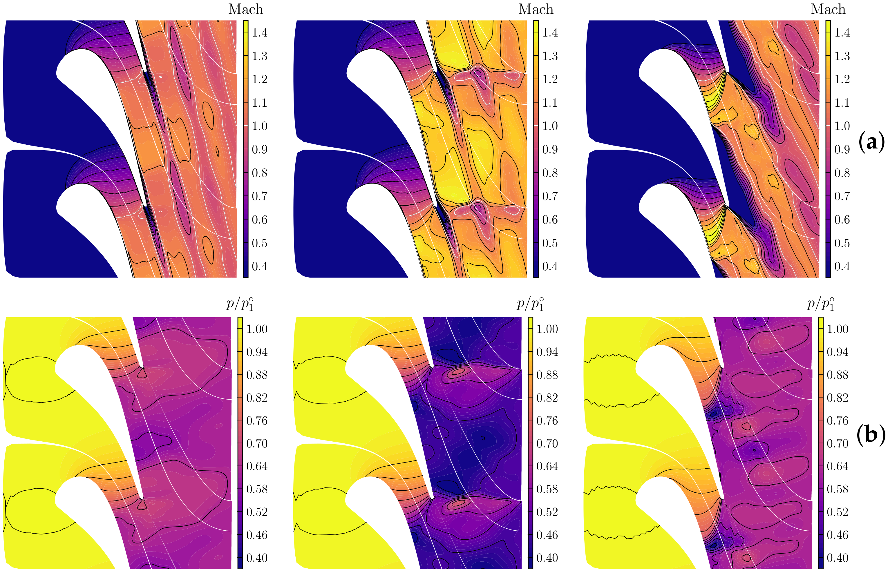
Hereafter, we discuss first-order flow statistics, computed as time and spanwise averages of the unsteady 3D LES results. The contours of the non-dimensional pressure, Mach number, fundamental derivative , and speed of sound are reported in Figure 4 for the three cases. For the IC1-LPR case (left column), the Mach number (row a) increases monotonically through the turbine vane as the pressure (row b) decreases, and reaches sonic conditions near the exit of the bladed portion, i.e., at the trailing edge on the pressure side. Due to the rounded shape of the trailing edge, the flow further expands downstream of the throat, reaching a maximum average value of approximately 1.1 close to the suction side of the trailing edge. Afterwards, the flow recompresses across the shock wave. Although the expansion starts in the BZT region (see the isocontours of the averaged , row c), the fundamental derivative becomes positive shortly downstream of the blade nose, and it remains lower than 1 throughout the expansion. This results in a reverse behavior of the speed of sound (shown in row d), which increases monotonically through the cascade up to the shock wave, instead of decreasing as in perfect gases. Nevertheless, the maximum Mach number in the cascade for the present molecularly complex working fluid is significantly higher than in air flow through the same geometry. Similar results were reported in [42] for an inviscid flow of propane through the same geometry with a similar pressure ratio. For case IC1-HPR, the Mach number (middle column, row a) also exhibits an overall increasing trend, although a local maximum is observed at the suction side, close to the mid-chord. This is due to the impingement of the right-running shock wave departing from the adjacent blade shortly downstream of the trailing edge. The latter is more clearly observed in the averaged pressure field (row b). In the trailing edge region, the flow first undergoes a supersonic expansion due to flow turning imposed by the rounded trailing edge, downstream of which a small recirculating region is created. At the end of the recirculation bubble, the supersonic flow coming from the suction and pressure sides re-aligns by means of left- and right-running shock waves, respectively. Similarly to the preceding case, is lower than one everywhere, and the speed of sound increases through the cascade (rows c and d). The supercritical case IC2-LPR (right column of Figure 4) exhibits significant differences with respect to the subcritical ones. An abrupt growth of the Mach number (row a) and a pressure drop (row b) are observed downstream of the channel throat due to a wave attached to the pressure side of the trailing edge. The fundamental derivative of gas dynamics (greater than one at the cascade inlet) becomes negative within the trailing edge wave system and then rises again, remaining less than one (the isocontour is highlighted in white). As a consequence, the speed of sound (row d) exhibits a non-monotonic behavior: It decreases at the beginning of the expansion while , and it increases afterwards.
Figure 5 provides a close-up view of the trailing edge region for the three cases. Average streamlines are superposed to the pressure field to highlight the recirculation bubble downstream of the trailing edge. The latter has a characteristic size of the order of the trailing edge thickness or less (for case IC2-LPR, see panel c), and it significantly deviates toward the suction side for the IC1-HPR and IC2-LPR cases due to the flow supersonic expansion around the rounded trailing edge at the pressure side. The computed base pressures (normalized with inlet total pressure) in the recirculation region are equal to 0.58, 0.45, and 0.64 for cases IC1-LPR, IC1-HPR, and IC2-LPR, respectively.
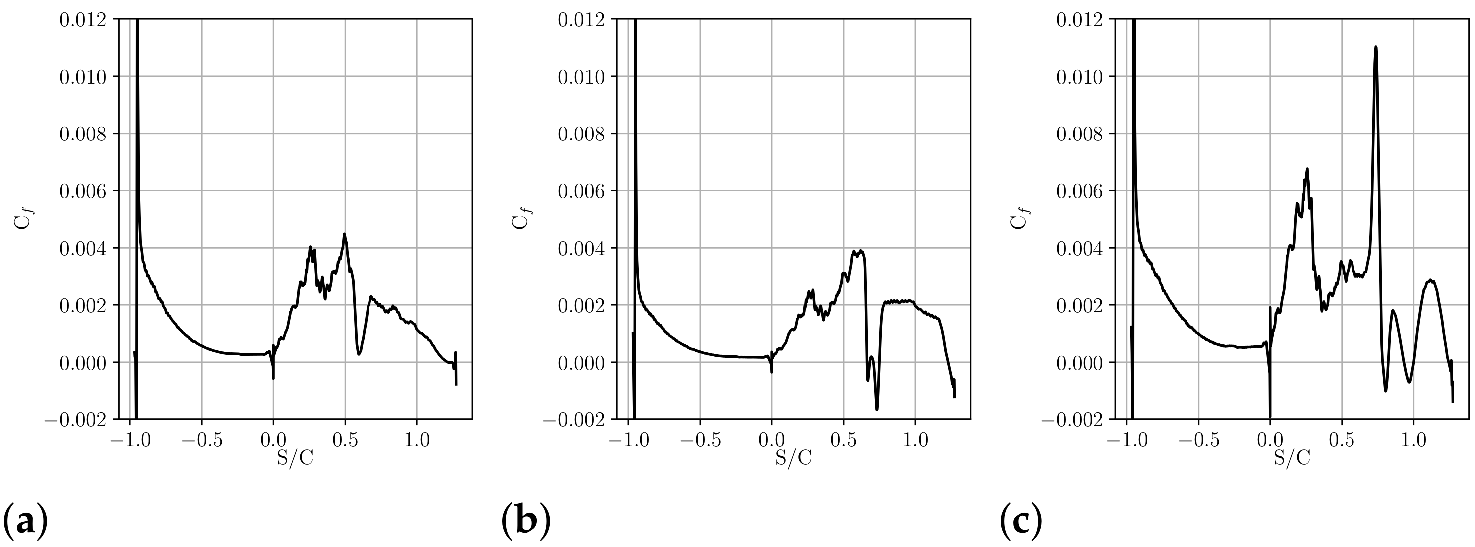
The averaged distributions of the skin friction coefficient () are reported in Figure 6 as a function of the curvilinear coordinate S along the blade wall ( at the leading edge, at the pressure side, and at the suction side), normalized with the chord C. The figure shows that, on average, the flow is fully attached for case IC1-LPR, except at the trailing edge (panel a). For case IC1-HPR, the interaction of the impinging right-running shock with the adjacent blade originates a small recirculation bubble for . Afterwards, the flow reattaches to separate again at the trailing edge. Finally, for IC2-LPR, the complex interactions of the non-classical waves with the boundary layer at the blade suction side lead to successive separation and reattachment of the boundary layer, which is otherwise attached almost everywhere.
For better understanding, the highly non-ideal case IC2-LPR is analyzed in some more detail in Figure 7, with a focus on the wave system associated with the trailing edge and wake region. The left column of Figure 7 displays maps of the averaged flow properties as well as three streamlines, denoted “line 1” (solid line), “line 2” (dashed line), and “line 3” (dotted line). The right column reports the evolution of various flow quantities along these streamlines. The fishtail-like system is composed of three main waves, denoted A, B, and C. Wave A departs from a location shortly upstream of the trailing edge at the pressure side. The second one, denoted B, is located roughly at two-thirds of the suction side. Finally, wave C also departs from the trailing edge system at the suction side and propagates downstream, interacting with the wake. The density distribution reported in row a shows that the flow undergoes an abrupt supersonic expansion across wave A and weak compressions across waves B and C (see also the Mach number distributions, row b). In particular, expansion A can be categorized as a mixed wave, which starts smoothly and then steepens abruptly to form an expansion shock as the fundamental derivative becomes negative (row c). Across the continuous expansion, the speed of sound and the Mach number experience a non-monotonic variation, as , initially greater than 1, decreases and finally reaches negative values. In particular, the Mach number initially increases (as in classical expansions) and then decreases. Across the expansion shock, the parameter J in Equation (2) is positive (row d), so the Mach number decreases. The flow remains supersonic downstream of A. The expansion wave is sharp in the vicinity of the trailing edge and tends to spread as it propagates through the channel. Finally, it impinges the lower blade, where it is reflected. At point B, the over-expanded supersonic flow recompresses through wave B, which interacts with the boundary layer. Accordingly, the density increases along streamline 1 and, to a significantly minor extent, along streamline 2 as they cross wave B. The latter develops in a region of positive and negative J, and it corresponds to a compression shock wave. Downstream of B, J changes its sign in the supersonic region above the boundary layer, while it is negative close to the suction surface of the blade. In the flow region next to point B, complex interactions with the expansion wave reflected from point A and with the wake are observed. The wake is deviated upwards by flow expansion at the pressure side of the trailing edge. This leads, in turn, to a compression at the suction side of the trailing edge, corresponding to wave C. Across C, flow properties vary smoothly. At points C, C, and C, the density increases and sound speed decreases. The Mach number decreases slightly close to the wall, i.e., along streamline 1, where , but exhibits a non-ideal behavior along streamlines 2 and 3, which cross a positive J region. Since wave C originates in the negative region near the trailing edge, we categorize it as a non-classical (smooth) compression wave. Such a wave also interacts with the wake and with the other waves downstream of the trailing edge, leading to a very complex unsteady wave pattern.
In order to assess the effects of the flow model on flow topology, RANS (or URANS) calculations were carried out for the same configurations. More precisely, steady RANS results are reported for IC1-LPR and IC1-HPR, while time-accurate (URANS) results are reported for IC2-LPR (as anticipated in Section 3). The pressure and Mach contours for the three cases are reported in Figure 8 for comparison. The RANS cases undergo a numerical transition at approximately one-third of the chord at the suction side. The overestimated growth of the turbulent boundary layers yields a restriction of the effective blade passage section and thicker wakes, substantially modifying the trailing edge shock system. By inspecting the same views for the LESs in Figure 4, we can see that the normal shock appearing in the case IC1-LPR at the suction side is much weaker and located earlier in the steady RANS, and the inclination of the fishtail shock attached to the trailing edge in the case IC1-HPR is altered. The URANS results or IC2-LPR strongly deviate from LES at the rear part of the suction side, due to the appearance of massive flow separation. Pressure distributions extracted at the first cell center off the wall for the LESs and RANS/URANS calculations are reported in Figure 9. The solutions are in quite fair agreement. The deviations observed in the laminar region at the suction side are due to small differences in the discretized blade geometry used for the two sets of calculations. In the figure, we also report results of inviscid flow calculations using C-grids of cells and a slightly modified trailing edge geometry (with a wedge). The overall agreement indicates that a large part of the flow is dominated by inviscid effects. In particular, the non-ideal expansion wave of case IC2-LPR is robustly predicted at by all models. Inviscid calculations fail in the rear part, predicting much stronger trailing edge shocks. We conclude that the trailing edge shock system is extremely sensitive to the model in use.
To further quantify the role of the model, we compute the loss coefficient, defined as:
where is the local isentropic temperature at downstream location 2, is the entropy difference, is the total enthalpy at the inlet, and the isentropic static enthalpy. The values for the LES, RANS, and inviscid calculations (computed as a mass-weighted section average at a section located approximately 0.1C downstream of the trailing edge) are reported in Table 4. These values must be taken with caution, and, in the absence of comparison with measurements or grid convergence of the LES simulations, they cannot be used to establish a hierarchy of performance among the different operating conditions. Nevertheless, they still bear interesting information about loss sensitivity to the different flow models. As expected, the inviscid flow model underestimates the losses for all cases except IC1-HPR: For this HPR case, shock losses (well captured by the inviscid model) are stronger and contribute significantly to the overall losses. On the contrary, RANS models overestimate the losses by predicting earlier fully turbulent boundary layers. The overestimation is dramatic for case IC2-LPR, for which a massive flow separation appears in the RANS solution. In the last line of Table 4, we report the loss coefficients calculated for air at the same PR and exit Reynolds number as IC1-LPR (i.e., case MUR129): is approximately one order of magnitude lower than for dense gas at the same pressure ratio due to the larger enthalpy drop (denominator of ). Similar observations can be found in [42] (for the same geometry and with propane as the working fluid). This case is subsonic for air, and the LES and RANS yield closer values than in the dense gas case, whereas the Euler simulation again predicts lower losses due to the absence of boundary layers. Overall, the results show the solution’s sensitivity to boundary-layer development and its interactions with the external flow.
4.2. Second-Order Statistics and Unsteady Flow Properties
Next, we focus on turbulent flow content and unsteady motions. Due to the interactions of the trailing-edge shock systems with the unsteady wake motions, both turbulent and inviscid contributions to the fluctuating field exist.
Figure 10 displays the instantaneous contours of the wall shear stress along the suction surface for the three cases. The distance to the leading edge is reported in terms of the normalized curvilinear abscissa . For case IC1-LPR, the shocks originating from the trailing edge and impinging the boundary layer of the adjacent blade are too weak to trigger transition. However, the perturbations are amplified downstream of the interaction point, leading to a roll-up of the boundary layer shortly upstream of the trailing edge. reaches a maximum downstream of the blade nose at , and the wall shear stress contours remain smooth all along the suction surface, the signature of streamwise rolls being visible only in the close vicinity of the trailing edge. An instantaneous separation bubble is also visible at , but was not observed in the time-averaged skin-friction profiles. This is likely due to boundary-layer interaction with impinging time-varying compression waves generated at the trailing edge of the upper blade, which may instantaneously sharpen into shocks. The flow ultimately transitions to turbulence in the wake. For case IC1-HPR, the oblique shock wave generated at the trailing edge impinges the boundary layer of the adjacent blade and leads to instantaneous boundary-layer separation () and transition to turbulence downstream of the interaction point for . Further downstream, the flow partly relaminarizes due to the favorable external pressure gradient, and a fully turbulent state is only achieved shortly upstream of the trailing edge (). The wall friction distribution for IC2-LPR is radically different from that of IC1-LPR due to the strongly non-ideal expansion. In this case, an abrupt variation of the wall shear stress is observed at location due to boundary-layer interaction with the sharp expansion wave. However, due to the favorable external pressure gradient, the transition is delayed to . As previously observed for IC1-HPR, the boundary layer partly relaminarizes further downstream under the effect of flow expansion, and finally transitions to turbulence close to the trailing edge ().
Although the details of the transition process and the position of the transition region may be sensitive to numerical resolution, the present calculations provide qualitative evidence that, at the selected Reynolds numbers, the flow is laminar over a significant portion of the blade surface and that shock-wave/boundary-layer interactions play a significant role in triggering transition.
The isocontours of resolved turbulent kinetic energy k based on time- and span-averaged velocity fluctuations are reported in Figure 11. High values of k are mostly concentrated in the turbulent wake and, according to the operating conditions, in the boundary layer at the rear part of the suction side. The regions of high k values observed in the inviscid core, especially for cases IC1-HPR and IC2-LPR, are not due to turbulence, but to unsteady motions of compression/expansion waves downstream of the trailing edge, leading to high velocity fluctuations. This effect is particularly noticeable for IC2-LPR due to the extreme sensitivity of the non-ideal wave system to small fluctuations of the local thermodynamic conditions.
To characterize the unsteady flow content, in Figure 12, we report the power spectral densities of the axial velocity component at three “numerical sensors” for the three LESs (shown in the inset). For IC1-LPR (panel a), the two sensors at the suction side of the blade do not exhibit any significant broadband content, confirming the laminar nature of the boundary layer at these stations. The dominant frequency detected in the signal of sensor one at a Strouhal number (defined as , where f is the frequency, is the trailing edge diameter, and is the outlet velocity) of about 0.013 is likely associated with the slow unsteady motion of compression waves impinging on the boundary layer. A marked peak at and its harmonics are observed for sensor 3, located just behind the trailing edge. Such a characteristic frequency is clearly representative of vortex shedding, for which the trailing edge thickness represents the relevant characteristic length [59]. Additionally note that the peak emerges from a broadband content, indicating that the flow behind the trailing edge is turbulent. For IC1-HPR (panel b), turbulent content is noticed much more upstream at the location of sensor 1. This station is downstream of the shock impinging on the suction side, where shock/boundary-layer interaction leads to flow transition. However, the spectra are more characteristic of transitional flow than fully developed turbulence for sensors 1 and 2. For this case as well, the spectrum at location 3 is marked by a sharp peak () corresponding to the vortex shedding frequency. For the highly non-ideal case (panel c), the first sensor is located shortly downstream of the mixed expansion-wave/boundary-layer interaction: The velocity spectrum exhibits a low-frequency peak corresponding to a Strouhal number of about and no broadband content. This confirms that the boundary layer is still laminar or at most transitional, and the low-frequency signal is associated with the unsteady motion of the expansion wave. The second sensor is located in the turbulent boundary layer, where half a decade of the inertial range following Kolmogorov’s −5/3 law is observed before the LES cut-off of the smallest scales. The third sensor, located in the wake, also returns a turbulent spectrum, but no well-defined inertial range −5/3 slope is observed. This is likely due to the vortex shedding from the bluff trailing edge that adds to the turbulent content, and corresponds to the "bump" in the spectrum observed around , before the LES cutoff. For all cases, no significant effect of the thermodynamic conditions on the characteristic frequency of the vortex shedding is observed, and the Strouhal numbers are in the range observed for transonic turbines using perfect gases [59].
5. Conclusions
Wall-resolved large eddy simulations of dense gas flows through a two-dimensional cascade of stator blades at highly non-ideal operating conditions were reported for the first time in the literature. The chosen cascade geometry corresponds to the VKI LS-89 configuration, which has been widely investigated in the literature for air flows, and is reasonably representative of a transonic ORC nozzle guide vane. The chosen working fluid, PP11, a heavy fluorocarbon, is well suited to investigate the influence of strong non-ideal effects on cascade performance. Several operating conditions, corresponding to subcritical and supercritical pressures at the turbine inlet, were considered, as well as two pressure ratios. The subcritical conditions led to mildly non-ideal gas dynamic effects in the flow field. On the contrary, dramatic deviations from the ideal-gas behavior were observed for the supercritical operating conditions. The latter included non-classical expansion and compression waves in complex interaction with the surrounding boundary layers and wakes. The use of a wall-resolved LES allows one to account for boundary-layer transition, which is seen to have a crucial role, at least at the moderate Reynolds number investigated in this study and in the absence of free-stream turbulence. According to the present simulations, the supercritical inlet operating conditions, which involved BZT effects in the trailing edge region, do not improve cascade losses, since the flow is severely over-expanded by non-classical waves, and it recompresses through a complex wave system downstream of the trailing edge, which is absent in the subcritical configuration at the same pressure ratio. Comparisons with the lower-fidelity, cheaper RANS models showed that RANS not only fails in predicting the transition point, but, more generally, leads to a significantly different boundary-layer development with an impact on the external flow. As a result, RANS is inaccurate in predicting cascade losses. Inviscid flow simulations were found to provide reasonable estimates of losses, at least for flow conditions dominated by shock losses. In future work, massive simulations with finer resolutions will help to get more quantitative insight into the complex mechanisms mentioned above. Massively parallel simulations will also enable the study of flows with higher Reynolds numbers, which are closer to conditions met in practical ORC applications, with specific a focus on the role of laminar–turbulent transition. LES studies of other working fluids and geometries are also planned.
Author Contributions
Conceptualization, P.C. and X.G.; methodology, J.-C.H., P.C., and X.G.; software, J.-C.H. and X.G.; data curation, J.-C.H.; writing—original draft preparation, J.-C.H. and P.C.; writing—review and editing, J.-C.H., P.C., and X.G.; supervision, P.C. and X.G.; project administration, P.C.; funding acquisition, P.C. All authors have read and agreed to the published version of the manuscript.
Funding
This study was funded by Direction Générale de l’Armement under PhD contract 2016-60-0043.
Institutional Review Board Statement
Not applicable.
Informed Consent Statement
Not applicable.
Data Availability Statement
Not applicable.
Acknowledgments
This work was granted HPC resources by the IDRIS National Scientific Computing Center, under the allocation number A0052A07332. This study was also funded by Direction Générale de l’Armement under PhD contract 2016-60-0043.
Conflicts of Interest
The authors declare no conflict of interest.
References
- Adam, A. Encyclopedia of Energy Technology and the Environment; John Wiley & Sons: New York, NY, USA, 1995; Volume 4, Chapter Organic Rankine Cycles. [Google Scholar]
- Schuster, A.; Karellas, S.; Kakaras, E.; Spliethoff, H. Energetic and economic investigation of organic Rankine cycle applications. Appl. Therm. Eng. 2009, 29, 1809–1817. [Google Scholar] [CrossRef] [Green Version]
- Chen, H.; Goswami, D.; Stefanakos, E. A review of thermodynamic cycles and working fluids for the conversion of low-grade heat. Sustain. Energy Rev. 2010, 14, 3059–3067. [Google Scholar] [CrossRef]
- Colonna, P.; Casati, E.; Trapp, C.; Mathijssen, T.; Larjola, J.; Turunen-Saaresti, T.; Uusitalo, A. Organic Rankine cycle power systems: From the concept to current technology, applications, and an outlook to the future. J. Eng. Gas Turbines Power 2015, 137, 100801. [Google Scholar] [CrossRef] [Green Version]
- Vescovo, R.; Spagnoli, E. High Temperature ORC Systems. Energy Procedia 2017, 129, 82–89. [Google Scholar] [CrossRef]
- Bini, R.; Colombo, D. Large multistage axial turbines. Energy Procedia 2017, 129, 1078–1084. [Google Scholar] [CrossRef]
- Schuster, A.; Karellas, S.; Aumann, R. Efficiency optimization potential in supercritical Organic Rankine Cycles. Energy 2010, 35, 1033–1039. [Google Scholar] [CrossRef]
- Lai, N.; Wendland, M.; Fischer, J. Working fluids for high-temperature organic Rankine cycles. Energy 2011, 36, 199–211. [Google Scholar] [CrossRef]
- Romei, A.; Vimercati, D.; Persico, G.; Guardone, A. Non-ideal compressible flows in supersonic turbine cascades. J. Fluid Mech. 2020, 882, A12. [Google Scholar] [CrossRef] [Green Version]
- Saleh, B.; Koglbauer, G.; Wendland, M.; Fischer, J. Working fluids for low-temperature Organic Rankine Cycles. Energy 2007, 32, 1210–1221. [Google Scholar] [CrossRef]
- Thompson, P. A fundamental derivative in gas dynamics. Phys. Fluids 1971, 14, 1843–1849. [Google Scholar] [CrossRef]
- Cramer, M.; Kluwick, A. On the propagation of waves exhibiting both positive and negative nonlinearity. J. Fluid Mech. 1984, 142, 9–37. [Google Scholar] [CrossRef]
- Cramer, M.; Best, L. Steady, isentropic flows of dense gases. Phys. Fluids A 1991, 3, 219–226. [Google Scholar] [CrossRef]
- Monaco, J.; Cramer, M.; Watson, L. Supersonic flows of dense gases in cascade configurations. J. Fluid Mech. 1997, 330, 31–59. [Google Scholar] [CrossRef]
- Brown, B.; Argrow, B. Application of Bethe-Zel’dovich-Thompson fluids in organic Rankine cycle engines. J. Propuls. Power 2000, 16, 1118–1124. [Google Scholar] [CrossRef]
- Congedo, P.; Corre, C.; Cinnella, P. Numerical investigation of dense-gas effects in turbomachinery. Comput. Fluids 2011, 49, 290–301. [Google Scholar] [CrossRef]
- Wheeler, A.; Ong, J. The role of dense gas dynamics on ORC turbine performance. In ASME Turbo Expo 2013; American Society of Mechanical Engineers: New York, NY, USA, 2013; Volume V002T07A030. [Google Scholar]
- Sciacovelli, L.; Cinnella, P. Numerical study of multistage transcritical organic Rankine cycle axial turbines. J. Eng. Gas Turbines Power 2014, 136, 082604-1–082604-14. [Google Scholar] [CrossRef] [Green Version]
- Cinnella, P.; Congedo, P. Inviscid and viscous aerodynamics of dense gases. J. Fluid Mech. 2007, 580, 179–217. [Google Scholar] [CrossRef]
- Colonna, P.; Harinck, J.; Rebay, S.; Guardone, A. Real-gas effects in organic Rankine cycle turbine nozzles. J. Propuls. Power 2008, 24, 282–294. [Google Scholar] [CrossRef]
- Bufi, E.; Cinnella, P. Preliminary design method for dense-gas supersonic axial turbine stages. J. Eng. Gas Turbines Power 2018, 140, 112605. [Google Scholar] [CrossRef]
- Rinaldi, E.; Pecnik, R.; Colonna, P. Unsteady operation of a highly supersonic organic Rankine cycle turbine. ASME J. Turbomach 2016, 138, 121010. [Google Scholar] [CrossRef]
- Obert, B.; Cinnella, P. Comparison of steady and unsteady RANS CFD simulation of a supersonic ORC turbine. Energy Procedia 2017, 129, 1063–1070. [Google Scholar] [CrossRef]
- Wilcox, D. Turbulence Modeling for CFD; DCW Industries: La Canada Flintridge, CA, USA, 2006. [Google Scholar]
- Durá Galiana, F.; Wheeler, A.; Ong, J. A study of trailing-edge losses in organic Rankine cycle turbines. ASME J. Turbomach 2016, 138, 121003. [Google Scholar] [CrossRef]
- Alshammari, F.; Pesyridis, A.; Karvountzis-Kontakiotis, A.; Franchetti, B.; Pesmazoglou, Y. Experimental study of a small scale organic Rankine cycle waste heat recovery system for a heavy duty diesel engine with focus on the radial inflow turbine expander performance. Appl. Energy 2018, 215, 543–555. [Google Scholar] [CrossRef]
- Zocca, M.; Guardone, A.; Cammi, G.; Cozzi, F.; Spinelli, A. Experimental observation of oblique shock waves in steady non-ideal flows. Exp. Fluids 2019, 60, 101. [Google Scholar] [CrossRef] [Green Version]
- Reinker, F.; Kening, E.; Passmann, M.; aus der Wiesche, S. Closed loop organic wind tunnel (CLOWT): Design, components and control system. Energy Procedia 2017, 129, 200–207. [Google Scholar] [CrossRef]
- Baumgartner, D.; Otter, J.; Wheeler, A. Closed loop organic vapor wind tunnel CLOWT: Commissioning and operational experience. In Proceedings of the 5th International Seminar on ORC Power Systems, Athens, Greece, 9–11 September 2019. [Google Scholar]
- Baumgartner, D.; Otter, J.; Wheeler, A. The Effect of Isentropic Exponent on Supersonic Turbine Wakes. ASME J. Turbom 2020, 142, 081007. [Google Scholar] [CrossRef]
- Beltrame, F.; Head, A.; Servi, C.; Pini, M.; Schrijer, F.; Colonna, P. First Experiments and Commissioning of the ORCHID Nozzle Test Section. NICFD: International Seminar on Non-Ideal Computational Fluid Dynamics. 2020. Available online: https://d2k0ddhflgrk1i.cloudfront.net/Websections/NICFD2020/Slides/Session%204%20-%20Fabio%20Beltrame.pdf (accessed on 31 January 2021).
- Sciacovelli, L.; Cinnella, P.; Content, C.; Grasso, F. Dense gas effects in inviscid homogeneous isotropic turbulence. J. Fluid Mech. 2016, 800, 140–179. [Google Scholar] [CrossRef] [Green Version]
- Sciacovelli, L.; Cinnella, P.; Gloerfelt, X. Direct numerical simulations of supersonic turbulent channel flows of dense gases. J. Fluid Mech. 2017, 821, 153–199. [Google Scholar] [CrossRef] [Green Version]
- Sciacovelli, L.; Cinnella, P.; Grasso, F. Small-scale dynamics of dense gas compressible homogeneous isotropic turbulence. J. Fluid Mech. 2017, 825, 515–549. [Google Scholar] [CrossRef] [Green Version]
- Sciacovelli, L.; Gloerfelt, X.; Passiatore, D.; Cinnella, P.; Grasso, F. Numerical investigation of high-speed turbulent boundary layers of dense gases. Flow Turbul. Combust. 2020, 105, 555–579. [Google Scholar] [CrossRef]
- Gloerfelt, X.; Robinet, J.C.; Sciacovelli, L.; Cinnella, P.; Grasso, F. Dense gas effects on compressible boundary layer stability. J. Fluid Mech. 2020, 893, A19. [Google Scholar] [CrossRef]
- Bhaskaran, R.; Lele, S. Large eddy simulation of free-stream turbulence effects on heat transfer to a high-pressure turbine cascade. J. Turbul. 2010, 11. [Google Scholar] [CrossRef]
- Collado, E.; Gourdain, N.; Duchaine, F.; Gicquel, L. Effects of free-stream turbulence on high pressure turbine blade heat transfer predicted by structured and unstructured LES. Int. J. Heat Mass Transf. 2012, 55, 5754–5768. [Google Scholar] [CrossRef]
- Wheeler, A.; Sandberg, R.; Sandham, N.; Pichler, R.; Michelassi, V.; Laskowski, G. Direct numerical simulations of a high-pressure turbine vane. ASME J. Turbomach 2016, 138, 071003–071009. [Google Scholar] [CrossRef]
- Segui, L.; Gicquel, L.; Duchaine, F.; de Laborderie, J. LES of the LS89 Cascade: Influence of Inflow Turbulence on the Flow Predictions. In European Conference on Turbomachinery Fluid Dynamics & Thermodynamics. 2017. Available online: https://www.euroturbo.eu/publications/proceedings-papers/ETC2017-159/ (accessed on 30 January 2021).
- Arts, T.; Lambert de Rouvroit, M.; Rutherford, A. Aero-thermal investigation of a highly loaded transonic linear turbine guide vane cascade. A test case for inviscid and viscous flow computations. In VKI Training Center for Experimental Aerodynamics Technical Note 174; Von Kármán Institute: Rhodes-Saint-Genese, Belgium, 1990. [Google Scholar]
- Harinck, J.; Guardone, A.; Colonna, P. The influence of molecular complexity on expanding flows of ideal and dense gases. Phys. Fluids 2009, 21, 086101. [Google Scholar] [CrossRef] [Green Version]
- Harinck, J.; Colonna, P.; Guardone, A.; Rebay, S. Influence of thermodynamic models in two-dimensional flow simulations of turboexpanders. ASME J. Turbomach 2010, 132, 011001. [Google Scholar] [CrossRef]
- Pichler, R.; Kopriva, J.; Laskowski, G.; Michelassi, V.; Sandberg, R. Highly resolved LES of a linear HPT vane cascade using structured and unstructured codes. In ASME Turbo Expo Conference; American Society of Mechanical Engineers: New York, NY, USA, 2016; Volume GT2016-49712. [Google Scholar]
- Schnerr, G.; Leidner, P. Internal flows with multiple sonic points. Acta Mech. 1994, 4, 147–154. [Google Scholar]
- Martin, J.; Hou, Y.C. Development of an equation of state for gases. AIChE J. 1955, 1, 142–151. [Google Scholar] [CrossRef] [Green Version]
- F2 Chemicals Ltd. FLUTEC Stability and Compatibility. Technical Article. Available online: http://f2chemicals.com/pdf/technical/Compatability.pdf (accessed on 31 January 2021).
- Hoarau, J.C.; Cinnella, P.; Gloerfelt, X. Large Eddy Simulation of dense gas flow around a turbine cascade. In Proceedings of the AIAA Aviation 2019 Forum, Dallas, TX, USA, 17–21 June 2019. AIAA Paper 2019-2843. [Google Scholar]
- Choi, H.; Moin, P. Grid-point requirements for large eddy simulation: Chapman’s estimates revisited. Phys. Fluids 2012, 24, 011702. [Google Scholar] [CrossRef]
- Chung, T.; Ajlan, M.; Lee, L.; Starling, K. Generalized multiparameter correlation for nonpolar and polar fluid transport properties. Ind. Eng. Chem. Res. 1988, 27, 671–679. [Google Scholar] [CrossRef]
- Cinnella, P.; Congedo, P. Aerodynamic performance of transonic Bethe–Zel’dovich–Thompson flows past an airfoil. AIAA J. 2005, 43, 370–378. [Google Scholar] [CrossRef]
- Visbal, M.; Morgan, P.; Rizzetta, D. An implicit LES approach based on high-order compact differencing and filtering schemes. In Proceedings of the 16th AIAA Computational Fluid Dynamics Conference, Orlando, FL, USA, 23–26 June 2003. AIAA Paper 2003-4098. [Google Scholar]
- Gloerfelt, X.; Cinnella, P. Large eddy simulation requirements for the flow over periodic hills. Flow Turbul. Combust. 2019, 103, 55–91. [Google Scholar] [CrossRef] [Green Version]
- Cinnella, P.; Content, C. High-order implicit residual smoothing time scheme for direct and large eddy simulations of compressible flow. J. Comput. Phys. 2016, 326, 1–29. [Google Scholar] [CrossRef]
- Hoarau, J.C.; Cinnella, P.; Gloerfelt, X. Large eddy simulation of turbomachinery flows using a high-order implicit residual smoothing scheme. Comput. Fluids 2020, 198, 104395. [Google Scholar] [CrossRef]
- Outtier, P.Y.; Content, C.; Cinnella, P.; Michel, B. The high-order dynamic computational laboratory for CFD research and applications. In Proceedings of the 21st AIAA Computational Fluid Dynamics Conference, San Diego, CA, USA, 24–27 June 2013. AIAA Paper 2013-2439. [Google Scholar]
- Kravchenko, A.; Moin, P. Numerical studies of flow over a circular cylinder at ReD = 3900. Phys Fluids 2000, 12, 403–417. [Google Scholar] [CrossRef]
- Cinnella, P.; Lerat, A. A fully implicit third-order scheme in time and space for unsteady turbulent compressible flow simulations. In Proceedings of the ECCOMAS: European Congress on Computational Methods in Applied Sciences and Engineering, Barcelona, Spain, 11–14 September 2000. [Google Scholar]
- Sieverding, C.H.; Richard, H.; Desse, J. Turbine Blade Trailing Edge Flow Characteristics at High Subsonic Outlet Mach Number. ASME J. Turbomach 2003, 125, 298–309. [Google Scholar] [CrossRef]
Figure 1.
Temperature–entropy chart for PP11 (Martin–Hou equation of state). Expansion lines for the three cascades considered in the study. The bold solid line corresponds to the liquid/vapor coexistence curve; the dashed line represents the contour; the dark gray region corresponds to the inversion zone; the light gray region corresponds to . Conditions at the turbine inlet and outlet are computed as average values on the inlet and outlet boundaries of the computational domain.

Figure 2.
Computational domain with boundary conditions (a), and close-up view of the grid (b), where one point out of four is represented.
Figure 2.
Computational domain with boundary conditions (a), and close-up view of the grid (b), where one point out of four is represented.

Figure 3.
Instantaneous iso-surface of the Q-criterion ( s) colored by the velocity magnitude (m/s), replicated three times in the spanwise direction, and snapshot of the relative density gradient in the background for cases IC1-LPR (low pressure ratio) (a), IC1-HPR (high pressure ratio) (b), and IC2-LPR (c).

Figure 4.
Isocontours of averaged quantities: Mach number (row (a)), pressure (row (b)), fundamental derivative (row (c)), and speed of sound (row (d)) for the cases IC1-LPR (left), IC1-HPR (middle), and IC2-LPR (right).
Figure 4.
Isocontours of averaged quantities: Mach number (row (a)), pressure (row (b)), fundamental derivative (row (c)), and speed of sound (row (d)) for the cases IC1-LPR (left), IC1-HPR (middle), and IC2-LPR (right).

Figure 5.
Close-up view of the trailing edge: isocontours of average pressure (background) and average stream lines for the cases IC1-LPR (a), IC1-HPR (b), and IC2-LPR (c).
Figure 5.
Close-up view of the trailing edge: isocontours of average pressure (background) and average stream lines for the cases IC1-LPR (a), IC1-HPR (b), and IC2-LPR (c).

Figure 6.
Wall distributions of the averaged skin friction coefficient for IC1-LPR (a), IC1-HPR (b), and IC2-LPR (c).
Figure 6.
Wall distributions of the averaged skin friction coefficient for IC1-LPR (a), IC1-HPR (b), and IC2-LPR (c).

Figure 7.
Maps of mean quantities (left) and their evolution along the three streamlines, labeled 1 to 3 (right) for case IC2-LPR: density (row (a)), Mach number (row (b)), (row (c)), and J (row (d)).
Figure 7.
Maps of mean quantities (left) and their evolution along the three streamlines, labeled 1 to 3 (right) for case IC2-LPR: density (row (a)), Mach number (row (b)), (row (c)), and J (row (d)).

Figure 8.
Reynolds-averaged Navier–Stokes (RANS) results for the Mach number (a) and normalized pressure (b). Cases IC1-LPR (left), IC1-HPR (middle), and IC2-LPR (right). For the latter case, the time-averaged unsteady RANS solution is presented.
Figure 8.
Reynolds-averaged Navier–Stokes (RANS) results for the Mach number (a) and normalized pressure (b). Cases IC1-LPR (left), IC1-HPR (middle), and IC2-LPR (right). For the latter case, the time-averaged unsteady RANS solution is presented.

Figure 9.
Normalized pressure distributions along the wall for cases IC1-LPR (left), IC1-HPR (middle), and IC2-LPR (right). denotes the normalized chordwise coordinate.
Figure 9.
Normalized pressure distributions along the wall for cases IC1-LPR (left), IC1-HPR (middle), and IC2-LPR (right). denotes the normalized chordwise coordinate.

Figure 10.
Instantaneous isocontours of the wall shear stress (Pa) for cases IC1-LPR (a), IC1-HPR (b), and IC2-LPR (c). Vertical dashed lines highlight the locations mentioned in the text.
Figure 10.
Instantaneous isocontours of the wall shear stress (Pa) for cases IC1-LPR (a), IC1-HPR (b), and IC2-LPR (c). Vertical dashed lines highlight the locations mentioned in the text.

Figure 11.
Isocontours of turbulent kinetic energy k for cases IC1-LPR (a), IC1-HPR (b), and IC2-LPR (c).
Figure 11.
Isocontours of turbulent kinetic energy k for cases IC1-LPR (a), IC1-HPR (b), and IC2-LPR (c).

Figure 12.
Velocity spectra for cases IC1-LPR (a), IC1-HPR (b), and IC2-LPR (c), evaluated at the three sensor locations shown in the inset.
Figure 12.
Velocity spectra for cases IC1-LPR (a), IC1-HPR (b), and IC2-LPR (c), evaluated at the three sensor locations shown in the inset.


Table 1.
Thermodynamic conditions for dense gas simulations. , , and are the total pressure, density, and temperature, respectively, , , and are the critical pressure, density, and temperature, is the fundamental derivative of gas dynamics, and is the Reynolds number. The indices 1 and 2 denote the inlet and outlet conditions, respectively.
| IC1-LPR | IC1-HPR | IC2-LPR | |
|---|---|---|---|
| 0.98 | 0.98 | 1.35 | |
| 0.62 | 0.62 | 1.47 | |
| 1.001 | 1.001 | 1.019 | |
| −0.093 | −0.093 | 6.706 | |
| 0.59 | 0.75 | 0.18 | |
| 1.58 | 2.10 | 1.58 | |
Table 2.
Thermodynamic properties of PP11 (CF): molecular weight , critical temperature , density , pressure , compressibility factor , and ratio of ideal-gas specific heat at a constant volume at the critical point over the gas constant .
Table 2.
Thermodynamic properties of PP11 (CF): molecular weight , critical temperature , density , pressure , compressibility factor , and ratio of ideal-gas specific heat at a constant volume at the critical point over the gas constant .
| 624.11 | 650.2 | 627.14 | 1.46 | 0.2688 | 97.3 |
Table 3.
Large eddy simulation (LES) parameters: , , and are the average sizes of the first cell close to the wall in wall units, is the time step, is the maximum number, and f.t.t. is the flow-through time.
Table 3.
Large eddy simulation (LES) parameters: , , and are the average sizes of the first cell close to the wall in wall units, is the time step, is the maximum number, and f.t.t. is the flow-through time.
| (s) | Time-Steps per f.t.t. | |||||
|---|---|---|---|---|---|---|
| IC1-LPR | 55 | 0.92 | 13 | 6.5 × | 7.0 | 13,000 |
| IC1-HPR | 99 | 1.54 | 24 | 6.5 × | 4.7 | 10,000 |
| IC2-LPR | 51 | 0.74 | 12 | 6.5 × | 5.4 | 15,000 |
Table 4.
Mass-weighted averaged loss coefficient at (where is the trailing edge coordinate) for various operating conditions and flow models.
Table 4.
Mass-weighted averaged loss coefficient at (where is the trailing edge coordinate) for various operating conditions and flow models.
| LES | RANS | Inviscid | |
|---|---|---|---|
| IC1-LPR | 0.82 × | 0.90 × | 0.69 × |
| IC1-HPR | 0.59 × | 0.82 × | 0.73 × |
| IC2-LPR | 0.53 × | 0.37 × | 0.45 × |
| MUR129 | 0.81 × | 0.82 × | 0.62 × |
Publisher’s Note: MDPI stays neutral with regard to jurisdictional claims in published maps and institutional affiliations. |
© 2021 by the authors. Licensee MDPI, Basel, Switzerland. This article is an open access article distributed under the terms and conditions of the Creative Commons Attribution (CC BY) license (http://creativecommons.org/licenses/by/4.0/).
Share and Cite
MDPI and ACS Style
Hoarau, J.-C.; Cinnella, P.; Gloerfelt, X. Large Eddy Simulations of Strongly Non-Ideal Compressible Flows through a Transonic Cascade. Energies 2021, 14, 772. https://0-doi-org.brum.beds.ac.uk/10.3390/en14030772
AMA Style
Hoarau J-C, Cinnella P, Gloerfelt X. Large Eddy Simulations of Strongly Non-Ideal Compressible Flows through a Transonic Cascade. Energies. 2021; 14(3):772. https://0-doi-org.brum.beds.ac.uk/10.3390/en14030772
Chicago/Turabian StyleHoarau, Jean-Christophe, Paola Cinnella, and Xavier Gloerfelt. 2021. "Large Eddy Simulations of Strongly Non-Ideal Compressible Flows through a Transonic Cascade" Energies 14, no. 3: 772. https://0-doi-org.brum.beds.ac.uk/10.3390/en14030772
Note that from the first issue of 2016, this journal uses article numbers instead of page numbers. See further details here.