
Simulation Analysis of CO2-EOR Process and Feasibility of CO2 Storage during EOR


1
Department of Petroleum and Gas Engineering and Energy, Faculty of Mining, Geology, and Petroleum Engineering, Pierottijeva 6, 10 000 Zagreb, Croatia
2
Independent Researcher, Santiago 8320000, Chile
*
Author to whom correspondence should be addressed.
Energies 2021, 14(4), 1154; https://0-doi-org.brum.beds.ac.uk/10.3390/en14041154
Submission received: 6 November 2020
/
Revised: 10 February 2021
/
Accepted: 17 February 2021
/
Published: 22 February 2021
(This article belongs to the Special Issue Enhanced Oil Recovery 2020)
Abstract
:In this study, oil production and retention were observed and compared in 72 reservoir simulation cases, after which an economic analysis for various CO2 and oil prices was performed. Reservoir simulation cases comprise different combinations of water alternating gas (WAG) ratios, permeabilities, and well distances. These models were set at three different depths; thus different pressure and temperature conditions, to see the impact of miscibility on oil production and CO2 sequestration. Those reservoir conditions affect oil production and CO2 retention differently. The retention trend dependence on depth was not monotonic—optimal retention relative to the amount of injected CO2 could be achieved at middle depths and mediocre permeability as well. Results reflecting different reservoir conditions and injection strategies are shown, and analysis including the utilization factor and the net present value was conducted to examine the feasibility of different scenarios. The analysis presented in this paper can serve as a guideline for multiparameter analysis and optimization of CO2-enhanced oil recovery (EOR) with a WAG injection strategy.
1. Introduction
1.1. Introduction
Enhanced oil recovery (EOR) with CO2 injection might be attractive because of the carbon dioxide retention in the reservoir [1], which provides a positive effect on the feasibility of CO2 storage and storage capacity obligations regarding the European Union international agreements within the climate change domain (Kyoto protocol from the year 1997 and the Paris climate agreement from the year 2015). Carbon Capture Utilization and Storage (CCUS) comes into focus when the possibilities of CO2 storage and reduction of storage cost are assessed. Although there are other utilization types, such as the utilization through beverage production or in agriculture, only the CO2 enhanced oil recovery (CO2-EOR) has been implemented at a commercial level on an industrial scale [2,3,4]. By injecting CO2 above the miscibility pressure (or minimum miscibility pressure (MMP)), microscopic displacement efficiency is improved due to viscosity reduction, oil swelling, lower interfacial tension, and a change in the density of oil and brine [5]. The efficiency of CO2 storage and CO2 utilization factors are not easy to determine. Static approximations are easier to implement, which usually leads to the use of statistical distributions and stochastic models [6,7,8], sometimes accompanied by numerical simulation and parameter analysis [9,10]. Recently the increasing number of published works have been focused on more complex CO2-EOR issues, such as injection rates of water and CO2 (water alternating gas (WAG) ratios), permeability anisotropy, the effect of different simulation cell size, etc. [11,12]. Oil recovery, injection cost, and the amount of carbon dioxide permanently stored can be optimized by the application of methods, which include water alternating gas (WAG) injection. Simulation of the WAG process can help establish optimal relation between the stated parameters.
The injection scheme of a typical CO2-EOR process can be classified according to:
- CO2 and oil miscibility
- miscible
- near-miscible
- immiscible
- injection type
- continuous gas injection (CGI)
- water alternating gas injection (WAG)
- simultaneous water and gas injection (SWAG)
There are no guidelines for the analysis or selection of WAG ratios, well distance, permeability, and time of primary production parameter based on multi-case simulation study as an input. The main reason for the absence of such guidelines, and in general, the reason such analysis has not been performed, is the long run-time of a typical compositional reservoir model and/or high dependence on geological and fluid properties in the case of complex heterogeneous reservoir models.
When CO2-EOR is performed, some of the CO2 retained in the reservoir. Depending on policies, in some cases (for example, the Weyburn Project), it is considered CO2 storage. For that reason, we use the word ‘CO2 retention’ as a synonym for storage. This paper brings a novel approach by a number of variations of the simulation parameters in a conceptual model (i.e., reservoir model and reservoir settings that are similar to real cases but generalized for parameter sensitivity analysis).
CO2 injection into a reservoir can be implemented in miscible and immiscible conditions, and the distinction between the two is defined by the minimum miscibility pressure. If the conditions are miscible, CO2 increases the oil mobility as it is dissolved in oil between the injector and the producer, and if the conditions are immiscible, there is no CO2 dissolution in oil, which means that CO2 flows much faster than oil toward the producers, causing lower oil recovery and higher production of previously injected CO2. The value of the minimum miscibility pressure depends mostly on oil composition and the reservoir temperature, and to determine the exact value of the minimum miscibility pressure, a detailed Pressure-Volume-Temperature (PVT) characterization of oil and the mixture of oil and CO2 is necessary.
1.2. Literature Review
Klinkenberg and Baylé [13] studied pore size distribution and miscible and immiscible fluid injection and concluded that the pore distribution affects miscible and immiscible displacement differently.
Hall and Geffen [14] made a mathematical model for saturation pressure, using fluid flow velocity (of liquid and gas), and liquid phase fraction during the two-phase flow. Additionally, pure compounds (methane, propane, butane, etc.) were used in the analysis, and for these compounds, zones of gaseous state, two-phase region, and region of 100% liquid saturation were identified.
Lacey, Draper, and Binder Jr [15] studied the length of the mixed zone in cores of different diameters. It was concluded that the length of the mixed zone is proportional to the area through which the fluids flow, but this cannot be a rule at the reservoir level.
In the 1960s, different authors studied mixing mechanisms experimentally [16,17,18]. Benham, Dowden, and Kunzman [16] analyzed the miscibility of rich gases with reservoir fluid by using ternary diagrams with methane, C2-C4, and C5+. They developed a correlation for maximum concentration of methane in miscible conditions as a function of temperature, pressure, the molecular weight of C5+, and the molecular weight of C2+.
Other authors ([19,20]) used somewhat different components in the ternary diagram, but oil composition is, in general, divided into components of lower molecular weight, components of the medium, and components of high molecular weight. Such estimates disregard the reservoir heterogeneity (heterogeneity of permeability, pore structures, and fluid saturations), which are mentioned by Deffrenne et al. [21].
Peaceman and Rachford [22] proposed a numerical method for the calculation of the 2D miscible displacement. A normal permeability distribution was generated by a random number method, and the model gave results in line with measured experimental data.
The Buckley–Leverett theory was used as a starting point for numerous modifications. Koval [23] published the most known paper regarding the semi-analytical description of miscible processes, in which a model was given describing solubility as a function of pore volumes injected using the K-factor method for Buckley–Leverett equation extension. He compared the results obtained by the suggested mathematical model with published data and got satisfactory results for heterogeneous systems of the horizontal reservoir in which fluids of different viscosities flow at different velocities—viscous fingering.
Fitch and Griffith [24] tested alternating water injection to achieve more efficient oil displacement. Simon and Graue [25] used experimental data regarding solubility, swelling, and CO2-oil system viscosity and gave a correlation for the prediction of these parameters as a function of oil viscosity and density. Different groups of authors developed more advanced mathematical, i.e., numerical simulation algorithms for CO2 injection [26,27,28,29].
Rathmell, Stalkup, and Hassinger [30] analyzed the relationship between recovery, core length, and injection pressure on 13 m long cores, 5 cm in diameter, with 0.27 porosity and 1D permeability. They assumed that at certain parts of the core, immiscible displacement occurs even when the injection pressure was higher than the MMP. They found that different flow velocities occur due to different oil and CO2 viscosities, which led to early CO2 breakthrough and this effect was more pronounced in experiments done on shorter cores. They concluded that oil recovery depends on oil vaporization and higher fractions of swelling.
Teja and Sandler [31] used the equation of state in which they adjusted the binary interaction coefficients and applied adequate mixing rules to simulate the density of the system/mixture CO2-oil, swelling factors, and CO2 solubility in oil at a given temperature.
Wang [32] designed special equipment for visual detection of miscibility conditions, and he showed that miscible, near-miscible, and immiscible displacement could occur at the same time during the CO2 injection. Among others, he also states that oil recovery cannot be the only criteria for MMP determination, and he proposed the determination of the optimal portion of CO2 in a WAG process.
Sigmund, Kerr, and MacPherson [33] gave a simple correlation for relative permeability determination in a slim-tube simulation model
where kro is the relative permeability of the liquid phase, and krg is the relative permeability of the gas phase.
Li and Luo [34] used displacement on core samples and slim-tube experiments to determine a correlation for relative permeabilities determination, which represents input data needed for simulation. They tried to correlate Corey’s exponents and the displacement pressure, but they concluded that relative permeability curves need to be adjusted by matching the simulation model with experimental data.
During WAG injection in water-wet rock, relative permeabilities depend on fluid saturation, saturation history, and the mobility will also depend on the interaction of viscosity, gravity, and capillary pressure [35]. Measurement of relative permeabilities during the three-phase displacement is usually not performed in a lab; therefore, it is common to measure relative permeabilities of a two-phase system, which is an acceptable input format for most commercial reservoir simulators.
Blunt [36] and Beygi et al. [37] reviewed most of so far suggested models for the determination of relative permeabilities of three-phase systems.
Jahangiri and Zhang [38] modified the second term of the optimization function (given by [39]) by introducing a mass of the stored CO2 (concerning overall CO2 mass storage capacity of the reservoir)
where w1 and w2 are weighted for oil recovery and CO2 storage in the objective function (dimensionless), NP is cumulative oil recovery (m3), OIP is oil in place (m3), is mass of CO2 stored (kg) is the total storage capacity of reservoir (kg).
However, the overall CO2 storage capacity of the reservoir is an uncertain parameter [40], and there is still no adequate optimization function for oil recovery and CO2 sequestration.
WAG injection can increase oil mobility, increase the displacement efficiency and the oil recovery, but the usual problem of a WAG process is the reduced displacement efficiency due to water blockage of CO2-oil contact [41], and that is the main reason why it is crucial to design the injection process correctly. Christensen, Stenby, and Skauge [41] gave an overview of 59 WAG projects. The expected recovery increase in some fields (South Swan, Slaughter Estate, Dollarhide, and Rangely Weber) is up to 20 %. Most of the WAG projects started in the tertiary phase of the exploitation. In other words, only recent WAG projects in the North Sea have started in the earlier exploitation phase. Eighty percent of projects are performed under miscible conditions, and the ratio of water and gas injection is mostly 1:1. Usual problems of a WAG process have been described, such as injectivity reduction, early water and gas breakthrough, corrosion, different temperatures of injected phases, hydrates formation, etc.
As a CO2-EOR process can be classified as immiscible, near-miscible, and miscible, the same classification may be applied to the WAG process. The water is used to maintain the reservoir pressure above the MMP, and to prevent the early breakthrough of CO2 to the production wells. Near miscible or immiscible WAG injection implies three-phase flow for which, no matter the longtime application of WAG processes in the world, there is still no complete understanding of changes in fluid composition which happen during such flow [41]. Extensive experimental and simulation research results have been published related to the mechanisms of displacement in the WAG process and water and gas injectivity [42,43,44,45,46,47,48,49,50,51,52]. Relative permeability models with different conditions of wettability for a three-phase system were developed along with hysteresis models necessary for the simulation of displacement in a WAG process [36,37,48,53,54,55,56,57,58,59,60].
Within the ESCOM (Evaluation System for CO2 Mitigation) project [61], numerous numerical simulations of hypothetical reservoirs were performed to define a mathematical model that would help to estimate the additional recovery and amount of CO2 retained in the reservoir. Different analyses identified the most important parameters, after which sensitivity analyses of these parameters were performed.
The amount of CO2 retained in the reservoir as part of the CO2-EOR project will become important in the EU if trading with European emission allowances (EUA) will be possible on the emission market, EU emissions trading system (EU ETS). Vulin et al. [62] investigate development of EU ETS, historical EUA price volatility, and trends correlated with price movements of natural gas, coal, and oil to forecast long-term EUA price probability using momentum strategy and geometric Brownian motion. Same as oil price, EUA price is influenced by policy, but some dependency on natural gas price and consumption was detected.
Sustainable development is based on finding the balance between industry growth and the environment, i.e., generating the lowest amount of damage while operating industrial activities efficiently.
To prove that CO2-EOR represents a feasible, mature, and clean carbon capture utilization and storage (CCUS) option, it is crucial to single out the most economically favorable option that can be applied considering the parameters crucial for CO2-EOR operations. Earnings of a CO2-EOR storage project come from oil production and avoided CO2. Avoided CO2 refers to the amount of CO2 retained in the reservoir during the EOR project, and this volume of CO2 can be considered as allowance and therefore used for trading in the EU ETS. Price of EUA on EU ETS can be observed as possible additional income besides oil production and on the other side highest costs are related to transport and injection of CO2 in CCUS projects.
Macintyre [63] examine different processes, instrumentation, material, and operating considerations connected to the design of CO2 compression, dehydration, and injection and concluded that the additional cost of corrosion prevention measures for CO2 injection is insignificant compared to the total implementation costs of the Joffre EOR project, which was the first miscible CO2-EOR project in Canada. He provided a real p-h diagram for the Joffre EOR project that requires only three stages of CO2 compression up to 130 bar.
McCollum and Ogden [64] gave some recommendations and examples of how to calculate compression and pumping power requirements emphasizing lower power requirements for pumping when the CO2 liquefies, i.e., for pressure and temperature conditions above CO2 critical values, including the Capital costs (CAPEX) estimation for pumping and compression phase of CO2 transport and injection.
Habel [65] observed the difference between reciprocating and centrifugal compressors for onshore CO2 CCUS applications with a recommendation for assessment of the required number of stages in case of centrifugal compressors that have many advantages over reciprocating compressors for flows over 12 kg/s and outlet pressure up to 250 bar.
Desai [66] made some general observations and challenges in the case of CO2 compression, including steps that can help companies to estimate their CO2 compressor requirements.
2. Materials and Methods
CO2 injection as a part of a CO2-EOR project, especially in the case of WAG injection, brings additional oil recovery (AR) accompanied by CO2 production, so it is important to consider produced CO2 quantities using retention, defined as
where represents CO2 injected through injection wells in Mt, and represents recycled CO2 in Mt.
CO2 produced at the production wells can be injected into the reservoir again after the separation process. This CO2 represents recycled CO2, which is injected together with the new CO2 in the next injection cycle. Since the results are sensitive to multiple parameters, and neither retention nor CO2 recycled does not show all the details of the injection process, we defined a dimensionless variable storability as:
Optimization of the CO2 injection in CO2-EOR projects can be evaluated through CO2 utilization factors (UF) since that factor is the ratio of utilized CO2 and produced oil, i.e., in this paper, CO2 UF was used and is previously defined by some authors ([67,68,69]) as
where refers only to the new CO2.
As for any other project, during the planning of an EOR project, it is common to develop an economical screen and perform discounted cash flow analysis, which is used as a standard method for deploying the time value of money in order to evaluate long-term developments, i.e., net present value (NPV) [70]
where Rt is the net cash flow during period t, i is the discount rate, and t is the number of time periods.
Reservoir simulations are performed with Schlumberger’s compositional numerical reservoir simulator E300, which uses the finite volume method to calculate the fluid flow.
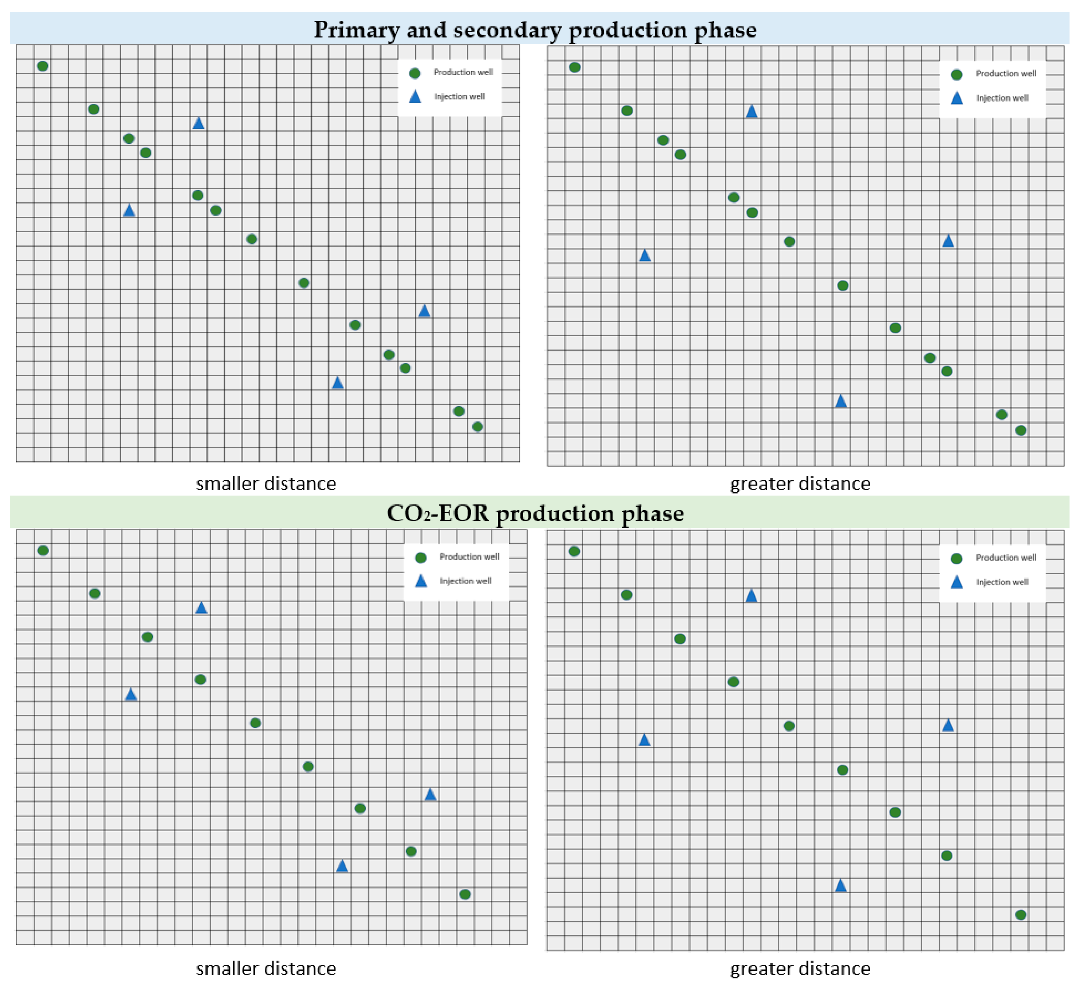
The reservoir has a closed boundary, and the selected grid for all models has 29 cells in the x-direction (NX = 29), 29 cells in the y-direction (NY = 29), and nine cells in the z-direction (NZ = 9), wherein the dimensions of the cells in the x and y directions are 50 m both, while the dimension of the cells in the z-direction is 10 m.
The model is based on the Miocene sandstones in the Sava depression, where porosities range from 21.5% to 23,6%, and in our conceptual models, we used 23.5%.
The simulations for this study were divided into three different models differentiated by depth, which are 715, 1545, and 1845 m. Each of these three listed models was then broken down for cases of the greater and smaller distance between production and injection wells and three different permeabilities (5 mD, 50 mD, and 250 mD), as shown in Table 1.
The differences between smaller and greater distance models per each production phase and model workflow are shown in Figure 1 and Figure 2.
Base model fluid production and pressure are matched to total oil production. No problems were encountered in simulation cases in control of Newton and linear iterations, nor in time truncation and convergence controls (Table 2). The PVT model was fine-tuned, and matching of the EOS to the laboratory tests is presented in [71].
The fluid composition and characterization for Model 3 were the same as in already published work [71]. In that work, detailed data on a PVT study, including a slim-tube test, were presented, and the resulting EOS matched the CO2 injection based on PVT laboratory data. PVT properties from that work were entered to the PVTp (Petroleum Experts software for PVT analysis), after which oil composition from the DLE (Differential Liberation) experiment at the pressure and temperature that corresponds to the initial pressure of each model was taken as the input composition for other two depths models (Table 3). Since the saturation pressure was 137 bar, the initial oil composition for Model 2 and Model 3 were the same. Model 3 corresponded to the oil reservoir in Sava Depression in terms of ranges of dynamic properties (mainly permeability and fluid properties).
Based on compositions from DLE, MMPs were determined for each base case, i.e., slim tube experiment was simulated in PVTp to obtain oil recovery for different injection pressures after 1.2 pore volumes of CO2 injected. MMP was defined as the intersection of two regression lines on a graph that relates the realized oil recovery and injection pressures. MMP for Model 2 remained similar as in Model 3, and in the case of Model 1, it was significantly lower (155 bar, Figure 3).
Three base cases (at three depths with respective initial reservoir pressure and then each with three different observation permeabilities) were simulated. Then cases were restarted after 10 years of primary production to simulate the secondary production phase for 48 years. After that, simulation cases were restarted again to simulate CO2-EOR that lasts fifteen years.
Maximum injection pressure for water and CO2 during the CO2 EOR phase was set to 30% higher than the initial reservoir pressure to simulate immiscible, near miscible and miscible conditions for used oil properties.
Different input values for prices of oil, price of EUA, and discount rates were considered to cover different earnings scenarios from more pessimistic to more optimistic scenarios (Table 4).
Capital costs (CAPEX) from the reviewed literature varied too significantly, and CAPEX was strongly site-specific. CAPEX for all the models was the same and taken from [72], since the models in this paper were similar to Ivanić field. The royalties, CAPEXs, operating expenses as an OPEX multiplicator (i.e., percentage of the produced oil value, representing processing and transportation costs to the mid-stream), the cost of water, and the CO2 injection used for economic evaluation are presented in Table 5.
CO2 injection costs in this paper were calculated according to [64], implying five stages of compression, i.e., CO2 injection costs are not fixed but depend on the injected amounts of CO2 and the injection pressure as a base for an estimation of the energy required for compression and charges for that energy.
3. Results
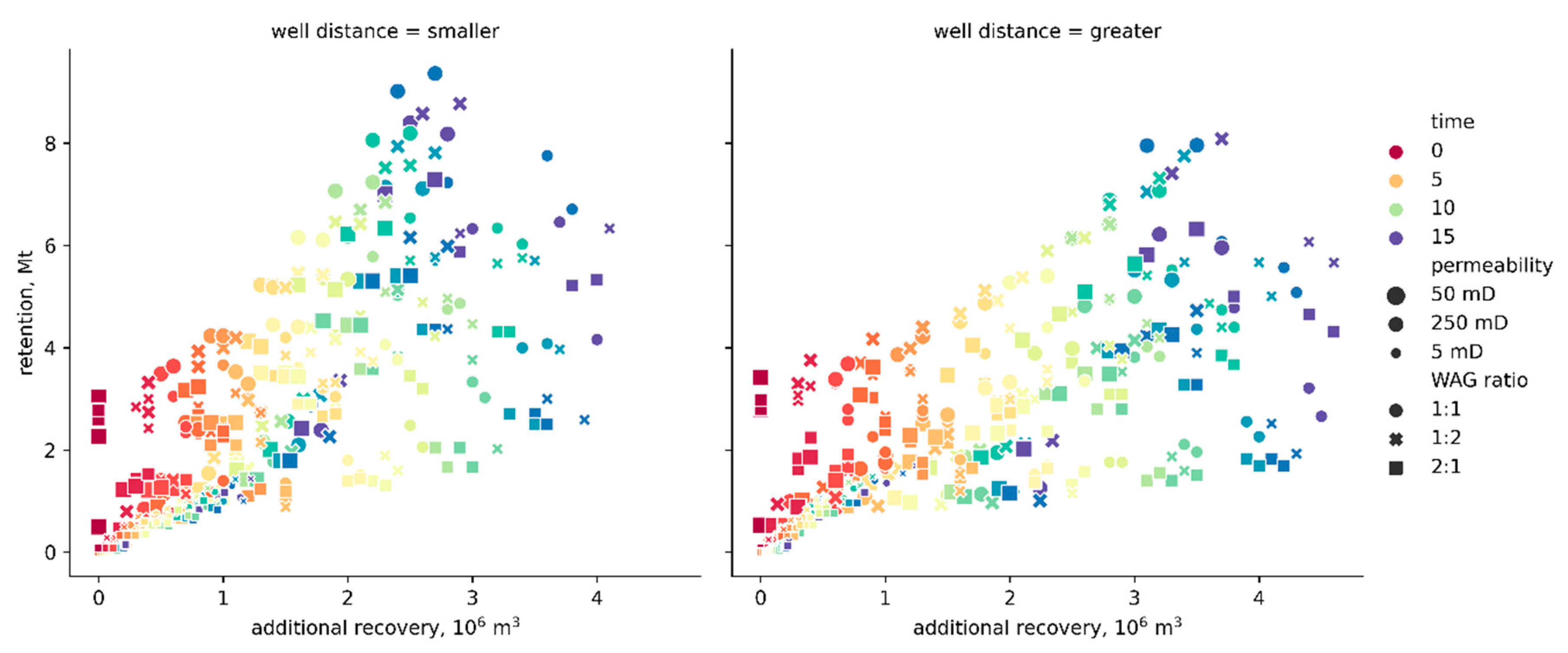
Additional recovery and retention were opposed parameters, i.e., maximum retention does not always bring maximum additional recovery (Figure 4). In the first years of CO2-EOR, retention to additional recovery ratio was higher, and with time, this ratio decreased.
The results show that if additional recovery was observed in relation to the injected pore volumes (PVs) of CO2 after 15 years of CO2-EOR, it was obvious that more PV could be injected in cases with a smaller distance between production and injection wells, which finally, allows more CO2 to be retained in a reservoir (Figure 5).
Retention was also highest for the cases with smaller well distances and a WAG ratio of 1:2 since much more CO2 could be injected in the case of smaller distances and a WAG ratio of 1:2 was the ratio in which CO2 was injected for the longest period (Figure 6).
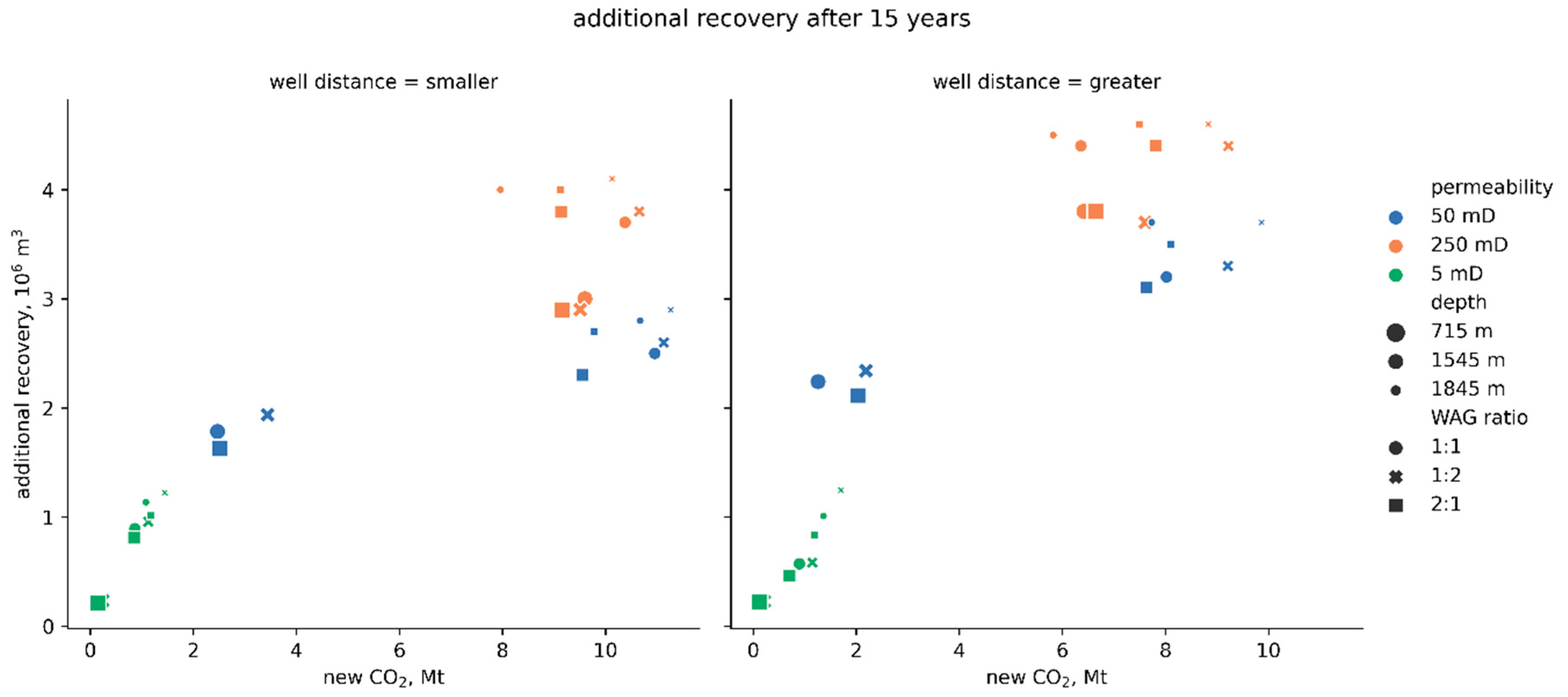
The results showed that if retention was observed relative to the new CO2, then the maximum retention was achieved at the greatest depths (Figure 7).
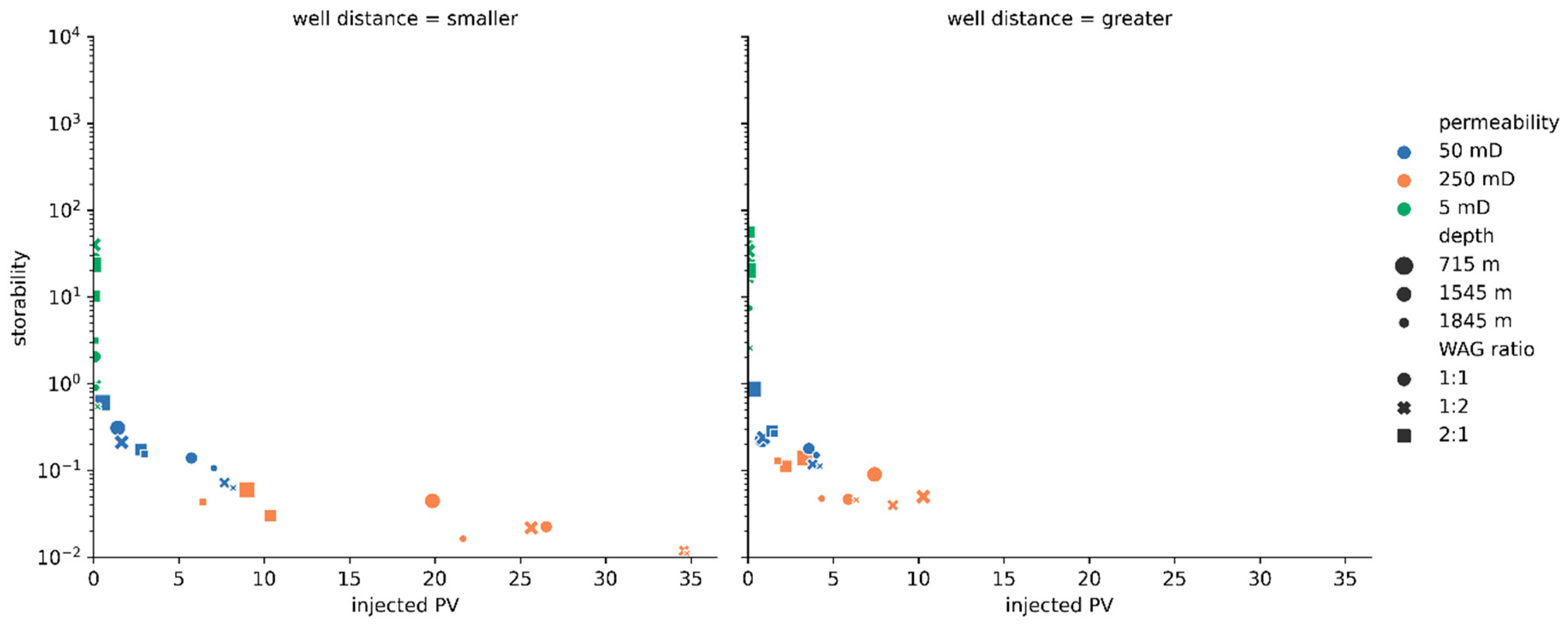
Higher storability was achieved at a greater well distance with less injected pore volumes, and the optimum WAG ratio was 2:1 (Figure 8).
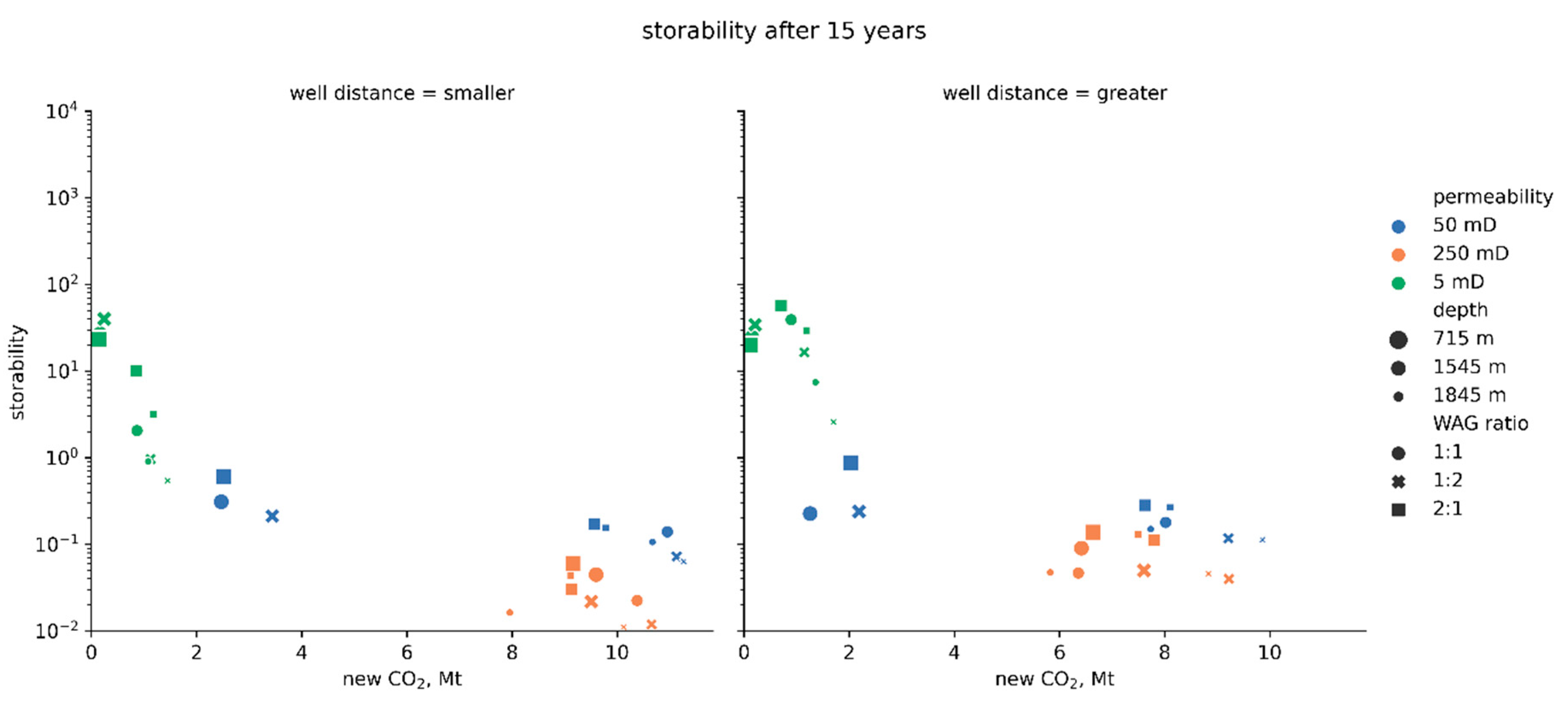
Storability was inversely proportional to permeability (highest storability in the case of lowest permeability), and the greatest storability was achieved for the smallest amounts of new CO2 brought to the system (Figure 9).
It should be noted that storage capacities for pure storage without EOR could not be achieved at the lowest permeabilities because of too high pressure (low injectivity) near the injection wells. The reason for that is that production wells act as some kind of "pressure release" wells during CO2-EOR.
There was a decreasing trend of storability with PV injected (Figure 8), which can be described by power-law functions (coefficients given in Table 6). Moreover, if permeability was included in the correlation, a decreasing trend could be described by the power-law function as well:
It should be noted that such a general correlation should be derived for each new reservoir setting (depth, well pattern, and oil composition) and each set of production parameters (WAG ratio, use of surfactants, and polymers).
Figure 10 shows two extreme cases of WAG injection. Left (Model 3) shows the CO2 molar density change under fully miscible conditions (greater depth), while on the right side, the same is shown for the case where the CO2 is injected under immiscible conditions (shallow reservoir). As CO2 can appear both in a gaseous and liquid state (supercritical is treated as a liquid in Eclipse), molar density is the best way to visualize the change of composition in space. Favorable cases (like that on the left, Figure 10) will result in greater areal sweep efficiency and consequently in higher CO2 retention (i.e., CO2 stored).
The utilization factor was significantly higher for cases with smaller well distances and was achieved for approximately the same injected PV’s as in the case of greater distance (Figure 11). The highest UF was achieved at some mediocre values of injected PV, mediocre permeabilities (k = 50 mD), and medium depths (1545 m). The smallest UF’s were achieved for lower depths and smallest permeability.
All previously presented parameters and their relationships should be presented concerning the economic value. The parameter that included both values added in terms of oil recovery and value-added in terms of CO2 permanently retained in the reservoir was UF.
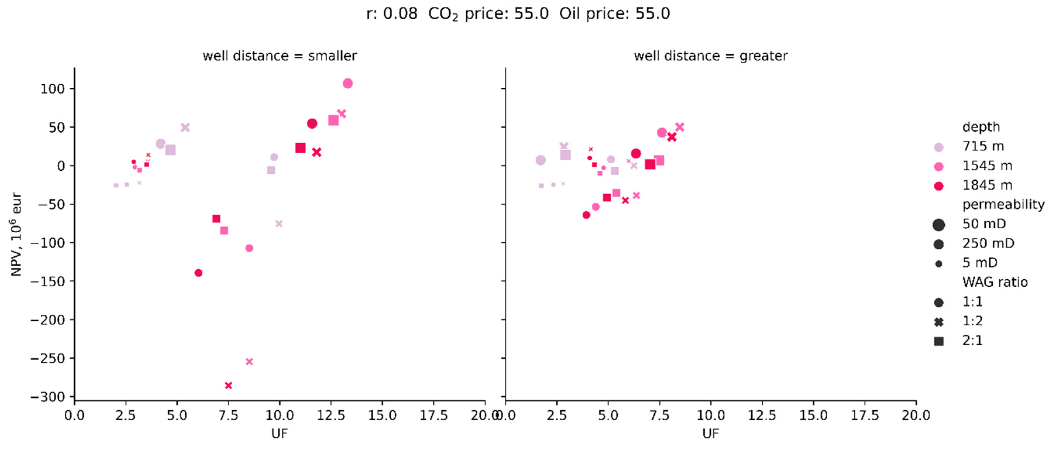
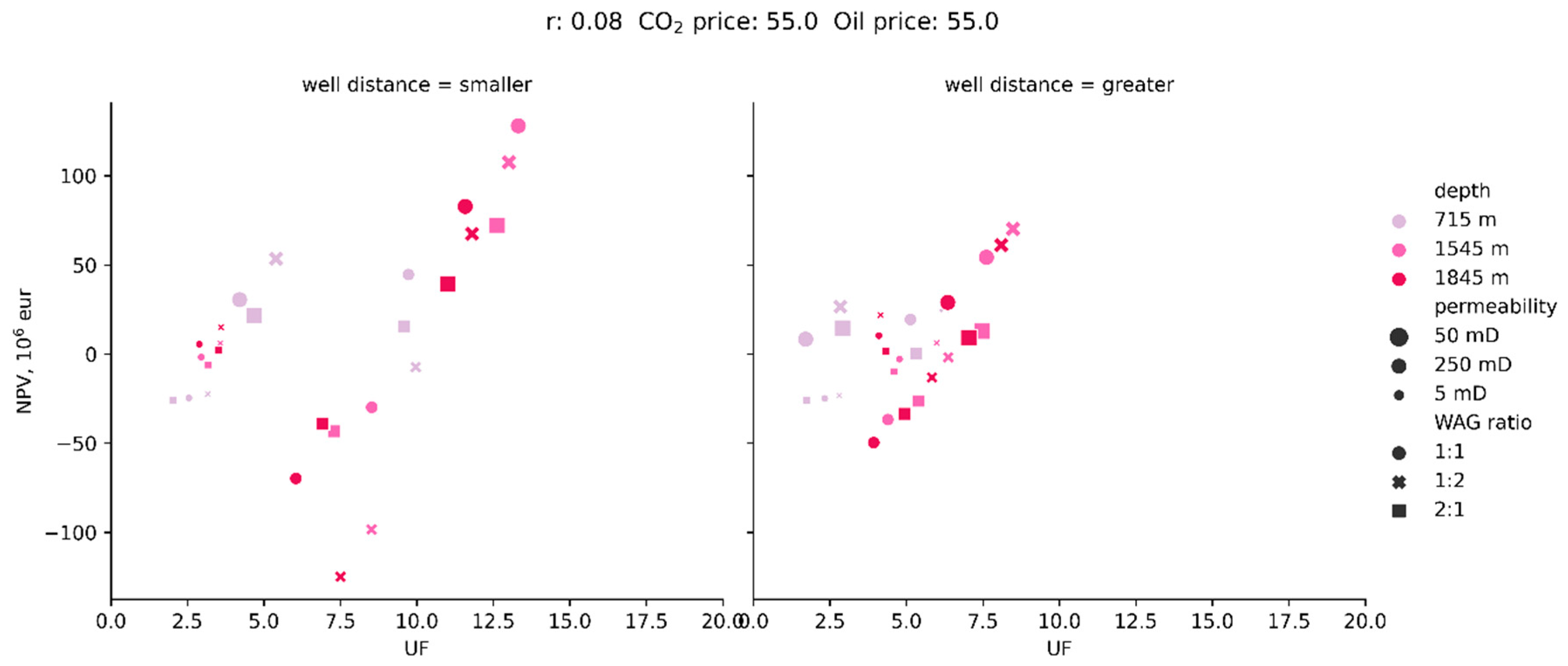
The realistic scenario is a scenario that implies current oil and EUA prices with the highest discount rate (r = 12%). The highest discount rate is selected because of the risk connected with oil and EUA price movements, which are hard to predict since those prices are usually influenced by the world’s political and economic situation. Also, electricity price varies differently throughout hours of the same day, with a maximum of 40 €/MWh and a minimum of 20 €/MWh, and that was the reason for calculating NPV for those two different scenarios of electricity price, i.e., costs of injection (Figure 12 and Figure 13).
The most optimistic case represents the highest prices of oil and carbon and the lowest discount rate (Figure 14 and Figure 15). On the other hand, the most pessimistic scenario had the lowest prices for carbon and oil and the highest discount rate (Figure 16 and Figure 17).
For optimistic scenarios, both electricity prices scenarios resulted in positive NPV value after 15 years of production (for electricity price 40 €/MWh maximum value is 106.8 million € and in case of 20 €/MWh maximum value was 128.1 million €). In a pessimistic scenario, it is not possible to achieve a positive NPV no matter the electricity price. Based on more calculated price scenarios (totaling 3888 cases of NPV observation after 15 years of CO2-EOR, Figure 18), more detailed insight into the influence of CO2 and oil price could be obtained.
NPVs in time, for realistic and optimistic scenarios and for both electricity prices are shown in Appendix A (Figure A1, Figure A2, Figure A3 and Figure A4). NPV in the first-time step was negative due to capital investment, but over time it moved towards higher/more positive values, depending on the observed scenarios.
The impact of the retention on NPV in the case of higher and lower electricity prices was not significant given that the impact of electricity prices did not relate to the retained CO2 but to the cost of injected CO2.
While high retention was generally connected with higher NPV, some optimal cases resulted in the highest NPVs, but not the highest additional recovery (Figure 19).
The parameter which relates to additional recovery and retention was the utilization factor (Figure 20). If the only profit from additional oil recovery was observed, the lowest values of UF would be favorable because, in such cases, the highest recoveries could be achieved with the smallest amounts of CO2 injected. NPV vs. UF showed a qualitatively similar trend to that in NPV vs. retention.
By including different CAPEXs in the analysis, a linear correlation between CAPEX and marginal CO2 price (Figure 21) was determined.
4. Discussion
Smaller well distance generally resulted in higher retention (Figure 4) because of the higher pressure between the injection and the production wells, which resulted in better mixing conditions and thus preventing viscous fingering of CO2.
Indicative was that the most injected PV’s correspond to the cases with smaller well distance and a 1:2 WAG ratio (Figure 5). Cases with the lowest permeabilities (5 mD) and depths were not among the best cases in terms of injectivity or additional recovery.
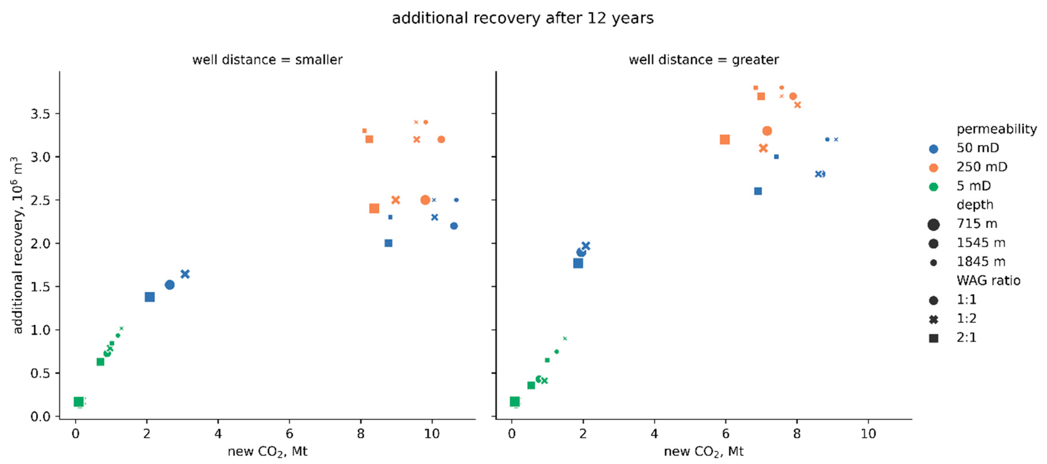
If the ratio of the new CO2 (which should be brought into the system) and recycled CO2 was observed concerning the additional recovery, it was evident that the highest permeability (250 mD) brought the highest recoveries and greatest depths also brought greater additional recovery while WAG ratio effects were not visible. If the parameters were observed versus time (Figure A5, Figure A6, Figure A7, Figure A8 and Figure A9), the distribution of all independent variables was qualitatively the same, but less CO2 should be brought to the system (more CO2 recycled) with time.
Storability was inversely proportional to permeability, depth (for the same permeability), and new CO2 brought to the system (Figure 8 and Figure 9).
The highest operating expenses which were not connected with oil production came from injection costs because of electricity consumption needed for compression (and less significant pumping) of required high quantities of CO2.
Depending on the applied, because of hourly electricity price fluctuation, electricity price maximum NPV at the end of EOR varies from 0.7 to 16.8 million €. The most cost-effective were those cases with the highest UF, a permeability of 50 mD, a WAG ratio of 1:1 or 1:2, at a depth of 1545 m for both electricity price cases. Generally, more feasible were cases with smaller well distance.
It is not possible to achieve a positive NPV if the CO2 price is below 15 €/t. Because of the hourly electricity price fluctuation and the special contracts between industrial consumers and the suppliers, the uncertainty of NPV value of the CO2-EOR will be especially high for the projects with a mediocre performance that might highly depend on electricity price (negative NPV values were more expressed than positive, Figure 18). By observing Figure 18, Figure 19 and Figure 20, from the similarity of the NPV vs. UF curve (which incorporated both the injected CO2 and the produced oil) and the NPV vs. retention curve, it was obvious that the oil production would affect NVP less than the CO2 retention.
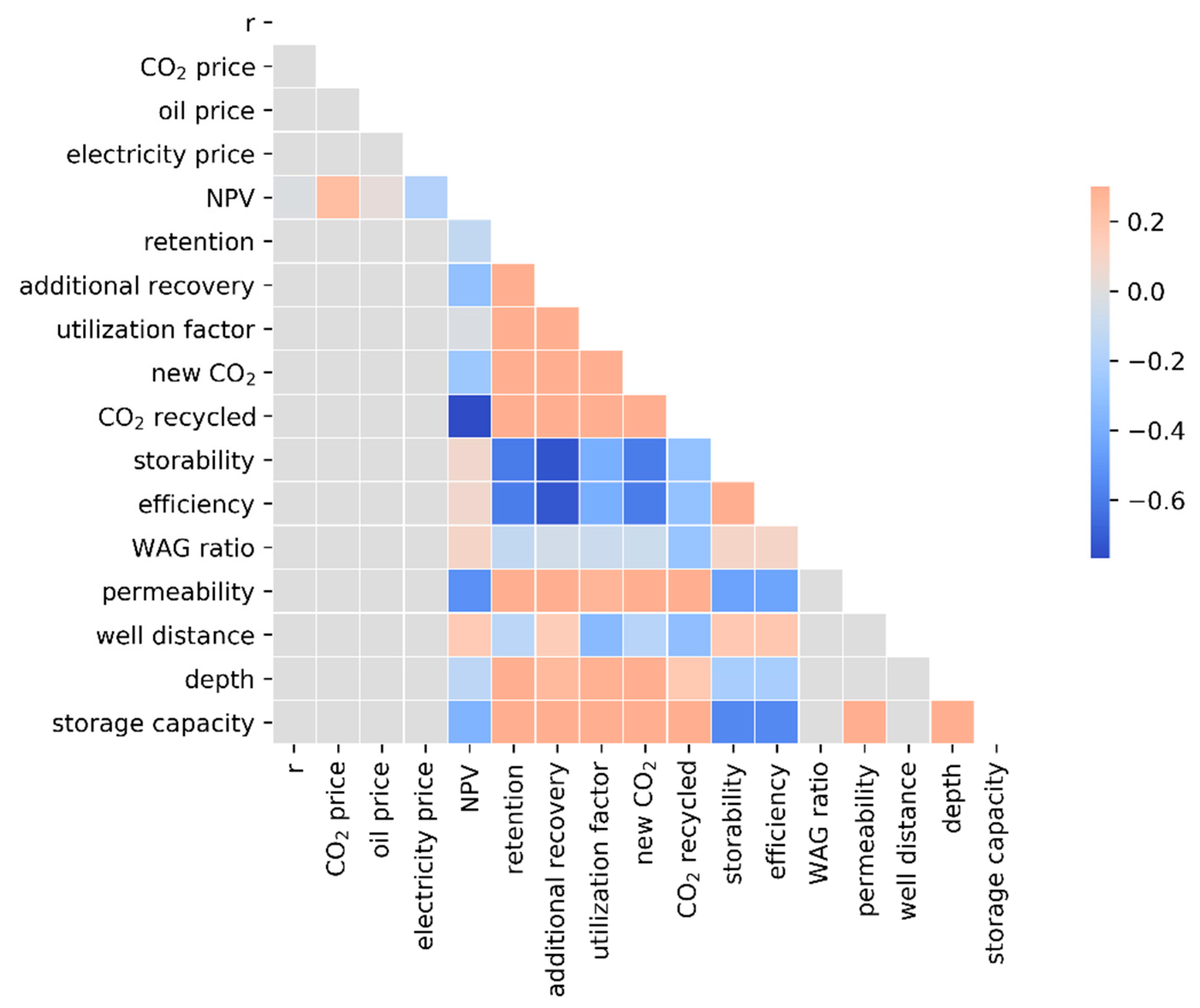
Discussed observations were put to statistical analysis of the strength of the relationship between the input and the resulting parameters. The mutual influence of the considered parameters was easiest to show using a diagonal correlation matrix (Figure 22). Values higher than zero indicated a positive correlation between observed parameters, and values less than zero represented a negative correlation. This statistical summary, as the quantitative benchmark of analyzed parameters, was in accordance with previously qualitatively detected relationships observed in Figure 4, Figure 5, Figure 6, Figure 7, Figure 8, Figure 9, Figure 10, Figure 11, Figure 12, Figure 13, Figure 14, Figure 15, Figure 16, Figure 17, Figure 18, Figure 19 and Figure 20.
A strong negative correlation of storability and additional recovery should be considered together with the positive correlation between depth and additional recovery since greater depths imply higher injection pressures connected with near miscible and miscible conditions for depths over 1545 m, i.e., more CO2 is dissolved in oil, therefore, more oil is produced, and less CO2 is retained. That was also the reason for the negative correlation found between storability and additional recovery. The reason for the strong negative correlation between NPV and CO2 recycled was the fact that if the CO2 is recycled, then there is a cost of injection, and there is no added value for retained CO2 (EUA price).
In general, in terms of NPV, many more parameters gave a negative correlation, and the most intense positive correlation referred to the CO2 price. As mentioned earlier in the results section, it was not possible to achieve a positive NPV if the CO2/EUA price was less than 15 €/t and with current prices of CO2 and oil, it was possible to achieve positive NPV with both maximum and minimum electricity price connected with costs of injection.
The main contribution of this paper is the incorporation of the WAG parameters and the reservoir conditions with the simultaneous economic feasibility assessment, which can serve as some guidelines for multiparameter analysis and optimization of the WAG process. However, considering the number of different values of each observed parameter, this analysis can be improved by introducing more permeability, well distance, and WAG ratio values.
5. Conclusions
The numerical simulation analysis, which consists of 54 different CO2-EOR injection cases (all combinations of three permeabilities, three depths, two well distances, and three WAG ratios) was taken as a basis for economic assessment (which consisted of three assumptions of interest rate, four CO2 prices, three oil prices, and two electricity prices), with the final number of cases for economic feasibility analysis 54 × 36 × 2 = 3888.
Considering so many cases was challenging, and it was necessary to create a structured query language (SQL) database of results and inputs and a system using Python code for data post-processing, economic and statistical analysis, and charting.
The following conclusions can be drawn:
- Retention of CO2 was affected by the distance between the injection and the production wells; smaller distances between them mean a higher volume of retained CO2 related to higher permeabilities and depth. The WAG ratio also had an impact on retention: ratios of 1:1 and 1:2 showed bigger retention caused by slug size of gas injection, which means more volume of the CO2 injected.
- When considering economic factors, well distance has an important effect on values of NPV. Higher values of NPV were attached to the smaller distances and cases with a permeability of 50 mD. For greater distances, the value of NPV was lower. UF will not be affected by oil and carbon prices, discount rates, and royalties. So, despite the market situation, having a lower UF with positive NPV is an indicator for perspective EOR strategies because of lower expenses for CO2 recycling.
- The most optimal case should fulfill the highest NPV and retention and the lowest UF. From the results of this investigation, an optimal case had a permeability of 50 mD, depth ranges between 1545 and 1845 m (from near miscible to miscible conditions), a WAG ratio of 1:2 was the best followed by 1:1. Regarding well distances, the choice should be based on the benefit from a higher NPV (risked to changing oil and carbon prices) with a higher UF or a moderately smaller NPV with a slightly lower UF. In the absence of more simulation results, it can be concluded that there are some optimal (not maximum or minimum) depth and permeability which will give the highest retention, additional recovery, and thus NPV.
- The maximum correlation value in the diagonal correlation matrix was around 0.2, and the minimum was around −0.6, i.e., negative correlations were much higher than positive ones, which implies that the CO2-EOR failure uncertainty will be smaller than the quality of the profit assessments.
The injection of the CO2 into a reservoir for EOR is economically feasible, and it has been applied for decades. Specifically, for the simulated conceptual models with some previously analyzed properties of oil fields in the Sava depression (Croatia), for the actual prices of carbon and oil, it is economically advantageous to develop new CO2-EOR projects, and it is clear that including CO2-EOR in EU ETS for the utilization and storage of CO2 (CCUS) would make a big difference in terms of CO2 storage, providing more assets for the application of advanced methods of monitoring and tracking CO2 over the entire process.
In addition to the CO2-EOR simulation cases, some pure storage cases were also simulated. For cases with 5 mD permeability, a too high value of pressure is quickly reached in the near-wellbore zone when the CO2 is injected for storage (there is no oil production and pressure release at production wells), and storage capacities in such cases are not significant and do not account as physically (or economically) feasible. The minimum difference between retention from CO2-EOR cases and storage capacity from pure storage cases is 1.68 Mt, and the maximum difference is 4.64 Mt (6.76 times more).
Finally, it is important to point out that as more oil is produced during CO2-EOR (CO2 utilization project), it is always possible to store more CO2 after the CO2-EOR ends, and most of the observed cases (more than 88%) showed the increase of storage capacity even after 15 years of CO2-EOR.
Author Contributions
Conceptualization, D.V. and M.A.; methodology, D.V.; software, D.V., M.A. and G.J.G.L.; validation, D.V.; formal analysis, D.V.; investigation, D.V., M.A., G.J.G.L. and L.J.; resources, D.V. and M.A.; data curation, M.A.; writing—original draft preparation, D.V., M.A., G.J.G.L., and L.J.; writing—review and editing, D.V., M.A., and L.J; visualization, D.V. and M.A.; supervision, D.V.; project administration, D.V.; funding acquisition, D.V. All authors have read and agreed to the published version of the manuscript.
Funding
This research received no external funding.
Informed Consent Statement
Informed consent was obtained from all subjects involved in the study.
Data Availability Statement
Data is contained within the article or supplementary material.
Acknowledgments
A part of this research was performed for additional analyses related to the EUH2020 (European Union’s Horizon 2020 Research and Innovation Programme) Strategy CCUS project, grant agreement No. 837754.
Conflicts of Interest
The authors declare no conflict of interest.
Appendix A
Figure A1.
Time versus NPV for the realistic scenario with 40 €/MWh electricity price.

Figure A2.
Time versus NPV for the realistic scenario with 20 €/MWh electricity price.

Figure A3.
Time versus NPV for the optimistic scenario with 40 €/MWh electricity price.

Figure A4.
Time versus NPV for the optimistic scenario with 20 €/MWh electricity price.

Figure A5.
Additional recovery versus new CO2 after 3 years of EOR.

Figure A6.
Additional recovery versus new CO2 after 6 years of EOR.

Figure A7.
Additional recovery versus new CO2 after 9 years of EOR.

Figure A8.
Additional recovery versus new CO2 after 12 years of EOR.

Figure A9.
Additional recovery versus new CO2 after 15 years of EOR.

References
- Dai, Z.; Middleton, R.; Viswanathan, H.; Fessenden-Rahn, J.; Bauman, J.; Pawar, R.; Lee, S.-Y.; McPherson, B. An Integrated Framework for Optimizing CO2 Sequestration and Enhanced Oil Recovery. Environ. Sci. Technol. Lett. 2014, 1, 49–54. [Google Scholar] [CrossRef]
- Ettehadtavakkol, A.; Lake, L.W.; Bryant, S.L. CO2-EOR and storage design optimization. Int. J. Greenh. Gas Control 2014, 25, 79–92. [Google Scholar] [CrossRef]
- Bachu, S. Identification of oil reservoirs suitable for CO 2 -EOR and CO 2 storage (CCUS) using reserves databases, with application to Alberta, Canada. Int. J. Greenh. Gas Control 2016, 44, 152–165. [Google Scholar] [CrossRef]
- Tapia, J.F.D.; Lee, J.-Y.; Ooi, R.E.; Foo, D.C.; Tan, R.R. Optimal CO2 allocation and scheduling in enhanced oil recovery (EOR) operations. Appl. Energy 2016, 184, 337–345. [Google Scholar] [CrossRef]
- Ghedan, S.G. Global Laboratory Experience of CO2-EOR Flooding. In Proceedings of the SPE/EAGE Reservoir Characterization and Simulation Conference, Abu Dhabi, United Arab Emirates, 19–21 October 2009. [Google Scholar] [CrossRef]
- Wei, N.; Li, X.; Fang, Z.; Bai, B.; Li, Q.; Liu, S.; Jia, Y. Regional resource distribution of onshore carbon geological utilization in China. J. CO2 Util. 2015, 11, 20–30. [Google Scholar] [CrossRef]
- Peck, W.D.; Azzolina, N.A.; Ge, J.; Gorecki, C.D.; Gorz, A.J.; Melzer, L.S. Best Practices for Quantifying the CO2 Storage Resource Estimates in CO2 Enhanced Oil Recovery. Energy Procedia 2017, 114, 4741–4749. [Google Scholar] [CrossRef]
- Azzolina, N.A.; Nakles, D.V.; Gorecki, C.D.; Peck, W.D.; Ayash, S.C.; Melzer, L.S.; Chatterjee, S. CO2 storage associated with CO2 enhanced oil recovery: A statistical analysis of historical operations. Int. J. Greenh. Gas Control 2015, 37, 384–397. [Google Scholar] [CrossRef] [Green Version]
- Karimaie, H.; Nazarian, B.; Aurdal, T.; Nøkleby, P.H.; Hansen, O. Simulation Study of CO2 EOR and Storage Potential in a North Sea Reservoir. Energy Procedia 2017, 114, 7018–7032. [Google Scholar] [CrossRef]
- Hosseininoosheri, P.; Hosseini, S.; Nuñez-López, V.; Lake, L. Impact of field development strategies on CO2 trapping mechanisms in a CO2–EOR field: A case study in the permian basin (SACROC unit). Int. J. Greenh. Gas Control. 2018, 72, 92–104. [Google Scholar] [CrossRef] [Green Version]
- Ren, B.; Duncan, I.J. Reservoir simulation of carbon storage associated with CO2 EOR in residual oil zones, San Andres formation of West Texas, Permian Basin, USA. Energy 2019, 167, 391–401. [Google Scholar] [CrossRef]
- Zhong, Z.; Liu, S.; Carr, T.R.; Takbiri-Borujeni, A.; Kazemi, M.; Fu, Q. Numerical simulation of Water-alternating-gas Process for Optimizing EOR and Carbon Storage. Energy Procedia 2019, 158, 6079–6086. [Google Scholar] [CrossRef]
- Klinkenberg, A.; Baylé, G.G. On the theory of adsorption chromatography for liquid mixtures: Part II: Binary mixtures over the full concentration range. Recl. des Trav. Chim. des Pays bas 1957, 76, 607–621. [Google Scholar] [CrossRef]
- Hall, H.N.; Geffen, T.M. A Laboratory Study of Solvent Flooding. Trans. AIME 1957, 210, 48–57. [Google Scholar] [CrossRef]
- Lacey, J.W.; Draper, A.L.; Binder, G.G., Jr. Miscible Fluid Displacement in Porous Media. Trans. AIME 1958, 213, 76–79. [Google Scholar] [CrossRef]
- Benham, A.; Dowden, W.; Kunzman, W. Miscible Fluid Displacement - Prediction of Miscibility. Trans. AIME 1960, 219, 229–237. [Google Scholar] [CrossRef]
- Adamson, J.A.; Flock, D.L. Prediction of Miscibility. J. Can. Pet. Technol. 1962, 1, 72–77. [Google Scholar] [CrossRef]
- Rutherford, W. Miscibility Relationships in the Displacement of Oil By Light Hydrocarbons. Soc. Pet. Eng. J. 1962, 2, 340–346. [Google Scholar] [CrossRef]
- Wilson, J.F. Miscible Displacement—Flow Behavior and Phase Relationships for a Partially Depleted Reservoir. Trans. AIME 1960, 219, 223–228. [Google Scholar] [CrossRef]
- Welge, H.; Johnson, E.; Ewing, S.J.; Brinkman, F. The Linear Displacement of Oil from Porous Media by Enriched Gas. J. Pet. Technol. 1961, 13, 787–796. [Google Scholar] [CrossRef]
- Deffrenne, P.; Marle, C.; Pacsirszki, J.; Jeantet, M. The Determination of Pressures of Miscibility. In Society of Petroleum Engineers of AIME, Proceedings of the Fall Meeting of the Society of Petroleum Engineers of AIME, Dallas, Texas, 10 August–11 October 1961; SPE International: Richardson, TX, USA, 1961. [Google Scholar] [CrossRef]
- Peaceman, D.W.; Rachford, H.J. Numerical Calculation of Multidimensional Miscible Displacement. Soc. Pet. Eng. J. 1962, 2, 327–339. [Google Scholar] [CrossRef]
- Koval, E. A Method for Predicting the Performance of Unstable Miscible Displacement in Heterogeneous Media. Soc. Pet. Eng. J. 1963, 3, 145–154. [Google Scholar] [CrossRef]
- Fitch, R.A. Experimental and Calculated Performance of Miscible Floods in Stratified Reservoirs. J. Pet. Technol. 1964, 16, 1289–1298. [Google Scholar] [CrossRef]
- Simon, R.; Graue, D.J. Generalized Correlations for Predicting Solubility, Swelling and Viscosity Behavior of CO2 -Crude Oil Systems. J. Pet. Technol. 1965, 17, 102–106. [Google Scholar] [CrossRef]
- Lanzz, R.B. Quantitative evaluation of numerical diffusion (truncation error). Soc. Pet. Eng. J. 1971, 11, 315–320. [Google Scholar] [CrossRef]
- Pope, G.; Nelson, R. A Chemical Flooding Compositional Simulator. Soc. Pet. Eng. J. 1978, 18, 339–354. [Google Scholar] [CrossRef]
- Van-Quy, N.; Simandoux, P.; Corteville, J. A Numerical Study of Diphasic Multicomponent Flow. Soc. Pet. Eng. J. 1972, 12, 171–184. [Google Scholar] [CrossRef]
- Graue, D.J.; Zana, E. Study of a Possible CO2 Flood in Rangely Field. J. Pet. Technol. 1981, 33, 1312–1318. [Google Scholar] [CrossRef]
- Rathmell, J.J.; Stalkup, F.I.; Hassinger, R.C. A Laboratory Investigation of Miscible Displacement by Carbon Dioxide. In Society of Petroleum Engineers of AIME, Proceedings of the Annual Fall Meeting of the Society of Petroleum Engineers of AIME, New Orleans, LA, USA, 3 October 1971; SPE International: Richardson, TX, USA, 1971. [Google Scholar] [CrossRef]
- Teja, A.S.; Sandler, S.I. A Corresponding States equation for saturated liquid densities. II. Applications to the calculation of swelling factors of CO2—crude oil systems. AIChE J. 1980, 26, 341–345. [Google Scholar] [CrossRef]
- Wang, G. Microscopic Investigation of CO2, Flooding Process. J. Pet. Technol. 1982, 34, 1789–1797. [Google Scholar] [CrossRef]
- Sigmund, P.M.; Kerr, W.; MacPherson, R.E. Laboratory and Computer Model Evaluation of Immiscible CO//2 Flooding in a Low-Temperature Reservoir. In Society of Petroleum Engineers of AIME, Proceedings of the SPE Enhanced Oil Recovery Symposium, Tulsa, Oklahoma, 22–24 April 1984; SPE International: Richardson, TX, USA, 1984; Volume 2, pp. 321–330. [Google Scholar] [CrossRef]
- Li, S.; Luo, P. Experimental and simulation determination of minimum miscibility pressure for a Bakken tight oil and different injection gases. Pet. 2017, 3, 79–86. [Google Scholar] [CrossRef]
- Marle, C. Multiphase Flow in Porous Media; Gulf Pub. Co.: Paris, France, 1981. [Google Scholar]
- Blunt, M.J. An Empirical Model for Three-Phase Relative Permeability. SPE J. 2000, 5, 435–445. [Google Scholar] [CrossRef]
- Beygi, M.R.; Delshad, M.; Pudugramam, V.S.; Pope, G.A.; Wheeler, M.F. Novel three-phase composi-tional relative permeability and three-phase hysteresis models. SPE J. 2015, 20, 21–34. [Google Scholar] [CrossRef]
- Jahangiri, H.R.; Zhang, D. Optimization of carbon dioxide sequestration and Enhanced Oil Recovery in oil reservoir. In Proceedings of the Society of Petroleum Engineers Western North American Regional Meeting 2010—In Collaboration with the Joint Meetings of the Pacific Section AAPG and Cordilleran Section GSA, Anaheim, CA, USA, 27–29 May 2010; Volume 2, pp. 902–910. [Google Scholar] [CrossRef]
- Kovscek, A.; Cakici, M. Geologic storage of carbon dioxide and enhanced oil recovery. II. Cooptimization of storage and recovery. Energy Convers. Manag. 2005, 46, 1941–1956. [Google Scholar] [CrossRef]
- Allinson, W.G.; Cinar, Y.; Neal, P.R.; Kaldi, J.; Paterson, L. CO2 storage capacity—Combining geology, engineering and economics. In Proceedings of the Society of Petroleum Engineers—SPE Asia Pacific Oil and Gas Conference and Exhibition 2010, Queensland, Australia, 18–20 October 2010; Volume 2. [Google Scholar] [CrossRef]
- Christensen, J.R.; Stenby, E.H.; Skauge, A. Review of WAG Field Experience. SPE Reserv. Eval. Eng. 2001, 4, 97–106. [Google Scholar] [CrossRef]
- Zekri, A.Y.; Natuh, A.A. Laboratory study of the effects of miscible WAG process on tertiary oil recovery. In Proceedings of the Abu Dhabi Petroleum Conference, Abu Dhabi, United Arab Emirates, 18–20 May 1992. [Google Scholar]
- Minssieux, L.; Duquerroix, J.P. WAG flow mechanisms in presence of residual oil. In Proceedings of the SPE Annual Technical Conference and Exhibition, New Orleans, LA, USA, 25–28 September 1994; pp. 145–150. [Google Scholar] [CrossRef]
- Skauge, A.; Serbie, K. Status of fluid flow mechanisms for miscible and immiscible WAG. In Proceeding of the Society of Petroleum Engineers - SPE EOR Conference at Oil and Gas West Asia 2014: Driving Integrated and Innovative EOR, Muscat, Oman, 31 March–2 April 2014; pp. 891–905. [Google Scholar] [CrossRef]
- Christensen, J.R.; Stenby, E.H.; Skauge, A. Compositional and relative permeability hysteresis effects on near-miscible WAG. In Proceedings of the SPE Symposium on Improved Oil Recovery, Tulsa, Oklahoma, 19–22 April 1998; Volume 1, pp. 233–248. [Google Scholar]
- Larsen, J.A.; Skauge, A. Simulation of the immiscible WAG process using cycle-dependent three-phase relative permeabilities. In Proceedings of the SPE Annual Technical Conference and Exhibition, Houston, TX, USA, 3–6 October 1999; Volume 1. [Google Scholar] [CrossRef]
- Christensen, J.R.; Larsen, M.; Nicolaisen, H. Compositional simulation of water-alternating-gas pro-cesses. In SPE Reservoir Engineering (Society of Petroleum Engineers), Proceeding of the SPE Annual Technical Conference and Exhibition, Dallas, TX, USA, 1–4 October 2000; SPE International: Richardson, TX, USA, 2000; pp. 307–317. [Google Scholar] [CrossRef]
- Egermann, P.; Vizika, O.; Dallet, L.; Requin, C.; Sonier, F. Hysteresis in three-phase flow: Experiments, modeling and reservoir simulations. In Proceedings of the European Petroleum Conference, Paris, France, 24–25 October 2000; pp. 173–186. [Google Scholar] [CrossRef]
- Sohrabi, M.; Tehrani, A.D.; Danesh, A.; Henderson, G.D. Visualization of Oil Recovery by Water-Alternating-Gas Injection Using High-Pressure Micromodels. SPE J. 2004, 9, 290–301. [Google Scholar] [CrossRef]
- Kulkarni, M.M.; Rao, D.N. Experimental investigation of miscible and immiscible Water-Alternating-Gas (WAG) process performance. J. Pet. Sci. Eng. 2005, 48, 1–20. [Google Scholar] [CrossRef]
- Spiteri, E.J.; Juanes, R. Impact of relative permeability hysteresis on the numerical simulation of WAG injection. J. Pet. Sci. Eng. 2006, 50, 115–139. [Google Scholar] [CrossRef]
- Fatemi Mobeen, S.; Sohrabi, M. Experimental investigation of near-miscible water-alternating-gas injection performance in water-wet and mixed-wet systems. SPE J. 2013, 18, 114–123. [Google Scholar] [CrossRef]
- Shahverdi, H.R.; Sohrabi, M. An Improved Three-Phase Relative Permeability and Hysteresis Model for the Simulation of a Water-Alternating-Gas Injection. SPE J. 2013, 18, 841–850. [Google Scholar] [CrossRef]
- Land, C.S. Calculation of Imbibition Relative Permeability for Two- and Three-Phase Flow From Rock Properties. Soc. Pet. Eng. J. 1968, 8, 149–156. [Google Scholar] [CrossRef]
- Stone, H.L. PROBABILITY MODEL FOR ESTIMATING THREE-PHASE RELATIVE PERVEABILITY. JPT J. Pet. Technol. 1970, 22, 214–218. [Google Scholar] [CrossRef]
- Stone, H. Estimation of Three-Phase Relative Permeability And Residual Oil Data. J. Can. Pet. Technol. 1973, 12, 53–61. [Google Scholar] [CrossRef]
- Killough, J.E. Reservoir Simulation with History-Dependent Saturation Functions. Soc. Pet. Eng. J. 1976, 16, 37–48. [Google Scholar] [CrossRef]
- Carlson, F.M. Simulation of relative permeability hysteresis to the nonwetting phase. In Proceedings of the SPE Annual Technical Conference and Exhibition, San Antonio, TX, USA, 4–7 October 1981. [Google Scholar] [CrossRef]
- Baker, L.E. THREE-PHASE RELATIVE PERMEABILITY CORRELATIONS. In Society of Petroleum Engineers of AIME, Proceedings of the SPE Enhanced Oil Recovery Symposium, Tulsa, Oklahoma, 16–21 April 1988; SPE International: Richardson, TX, USA, 1988; pp. 539–554. [Google Scholar] [CrossRef]
- Larsen, J.; Skauge, A. Methodology for Numerical Simulation with Cycle-Dependent Relative Permeabilities. SPE J. 1998, 3, 163–173. [Google Scholar] [CrossRef] [Green Version]
- Vulin, D.; Karasalihović Sedlar, D.; Saftić, B.; Perković, L.; Macenić, M.; Jukić, L.; Lekić, A.; Arnaut, M. ESCOM—Evaluation system for CO2 mitigation. In Proceedings of the 3rd International Scientific Conference on Economics and Management: How to Cope With Disrupted Times—EMAN 2019, Ljubljana, Slovenija, 28 March 2019. [Google Scholar]
- Vulin, D.; Arnaut, M.; Sedlar, D.K. Forecast of long-term EUA price probability using momentum strategy and GBM simulation. Greenh. Gases: Sci. Technol. 2019, 10, 230–248. [Google Scholar] [CrossRef]
- MacIntyre, K. Design Considerations For Carbon Dioxide Injection Facilities. J. Can. Pet. Technol. 1986, 25. [Google Scholar] [CrossRef]
- McCollum, J.M.; Ogden, D.L. Techno-Economic Models for Carbon Dioxide Compression, Transport, and Storage & Correlations for Estimating Carbon Dioxide Density and Viscosity; UC Davis: Institute of Transportation Studies: Davis, CA, USA, 2006. [Google Scholar]
- Habel, R. Advanced Compression Solutions for CCS, EOR and Offshore CO2; OTC: Rio de Janeiro, Brazil, 2011. [Google Scholar] [CrossRef]
- Desai, M.G. Specifying Carbon Dioxide Centrifugal Compressor. SPE Prod. Oper. 2018, 33, 313–319. [Google Scholar] [CrossRef]
- Olalotiti-Lawal, F.; Onishi, T.; Kim, H.; Datta-Gupta, A.; Fujita, Y.; Hagiwara, K. Post-Combustion Carbon Dioxide Enhanced-Oil-Recovery Development in a Mature Oil Field: Model Calibration Using a Hierarchical Approach. SPE Reserv. Evaluation Eng. 2019, 22, 998–1014. [Google Scholar] [CrossRef]
- Saini, D.; Jiménez, I. Evaluation of CO2-EOR and Storage Potential in Mature Oil Reservoirs. In Proceedings of the SPE Western North American and Rocky Mountain Joint Meeting, Denver, CO, USA, 16–18 April 2014. [Google Scholar] [CrossRef]
- Pasumarti, A.; Mishra, S.; Ganesh, P.R.; Mawalkar, S.; Burchwell, A.; Gupta, N.; Raziperchikolaee, S.; Pardini, R. Practical Metrics for Monitoring and Assessing the Performance of CO2-EOR Floods and CO2 Storage in Mature Reservoirs. In Proceedings of the SPE Eastern Regional Meeting, Canton, OH, USA, 13–15 September 2016. [Google Scholar] [CrossRef]
- Salem, S.; Moawad, T. Economic Study of Miscible CO2 Flooding in a Mature Waterflooded Oil Reservoir. In Proceedings of the SPE Saudi Arabia Section Technical Symposium and Exhibition, Al-Khobar, Saudi Arabia, 19–22 May 2013. [Google Scholar] [CrossRef]
- Vulin, D.; Gaćina, M.; Biličić, V. Slim-tube simulation model for CO2 injection eor. Rudarsko-geološko-naftni zbornik 2018, 33, 37–48. [Google Scholar] [CrossRef] [Green Version]
- Novosel, D. Učinak ugljičnog dioksida u tercijarnoj fazi iskorištavanja naftnih ležišta polja Ivanić. Ph.D. Thesis, Faculty of Mining, Geology and Petroleum Engineering (University of Zagreb), Zagreb, Croatia, 2009. [Google Scholar]
Figure 1.
Models grid scheme. CO2-EOR: CO2-enhanced oil recovery.

Figure 2.
Model development workflow.

Figure 3.
Minimum miscibility pressure for (a) Model 1 and (b) Model 2.

Figure 4.
Retention versus additional recovery.

Figure 5.
Additional recovery versus injected pore volumes (PVs) after 15 years of EOR.

Figure 6.
Retention versus injected pore volumes after 15 years of EOR.

Figure 7.
Retention versus new CO2 after 15 years of EOR.

Figure 8.
Storability versus injected pore volumes after 15 years of EOR.

Figure 9.
Storability versus new CO2 after 15 years of EOR.

Figure 10.
CO2 molar density change during WAG injection with a WAG ratio of 1:1.


Figure 11.
Utilization factor (UF) versus injected PV after 15 years of EOR.

Figure 12.
Net present value (NPV) versus UF for the realistic scenario at the end of EOR with 40 €/MWh electricity price.
Figure 12.
Net present value (NPV) versus UF for the realistic scenario at the end of EOR with 40 €/MWh electricity price.

Figure 13.
NPV versus UF for the realistic scenario at the end of EOR with 20 €/MWh electricity price.
Figure 13.
NPV versus UF for the realistic scenario at the end of EOR with 20 €/MWh electricity price.

Figure 14.
NPV versus UF for the optimistic scenario at the end of EOR with 40 €/MWh electricity price.
Figure 14.
NPV versus UF for the optimistic scenario at the end of EOR with 40 €/MWh electricity price.

Figure 15.
NPV versus UF for the optimistic scenario at the end of EOR with 20 €/MWh electricity price.
Figure 15.
NPV versus UF for the optimistic scenario at the end of EOR with 20 €/MWh electricity price.

Figure 16.
NPV versus UF for the pessimistic scenario at the end of EOR with 40 €/MWh electricity price.
Figure 16.
NPV versus UF for the pessimistic scenario at the end of EOR with 40 €/MWh electricity price.

Figure 17.
NPV versus UF for the pessimistic scenario at the end of EOR with 20 €/MWh electricity price.
Figure 17.
NPV versus UF for the pessimistic scenario at the end of EOR with 20 €/MWh electricity price.

Figure 18.
NPV versus retention after 15 years of CO2 EOR for different discount rates, oil and CO2 prices, and two different electricity prices (compression costs).
Figure 18.
NPV versus retention after 15 years of CO2 EOR for different discount rates, oil and CO2 prices, and two different electricity prices (compression costs).

Figure 19.
NPV vs. additional recovery after 15 years of CO2-EOR.

Figure 20.
NPV vs. additional recovery after 15 years of CO2-EOR.

Figure 21.
Marginal CO2 price versus CAPEX.

Figure 22.
Diagonal correlation matrix.


Table 1.
Parameter matrix for numerical simulation case-sensitivity analysis.
| Model 1 | Model 2 | Model 3 | |
|---|---|---|---|
| Depth (m) | 715 | 1545 | 1845 |
| WAG Ratio | 1:1, 1:2, 2:1 | 1:1, 1:2, 2:1 | 1:1, 1:2, 2:1 |
| Initial Datum Pressure (bar) | 78 | 164 | 195 |
| Reservoir Temperature (°C) | 60 | 96.6 | 110 |
| Permeability (mD) | 5, 50, and 250 | 5, 50, and 250 | 5, 50, and 250 |
| Distance between injection and production wells | Smaller and Greater | Smaller and Greater | Smaller and Greater |
Table 2.
Solver constraints and convergence controls used in the simulator.
| Time truncation and convergence controls | |
| Target TTE (time truncation error): | 0.2 |
| Maximum non-linear convergence error: | 0.001 |
| Maximum material balance error: | 0.000001 |
| Target reduction in the square of the relative residual norm in the linear solver: | Improvement by a factor of 1 × 10⁻¹⁰ in the square of the residual |
| Maximum TTE (Time Truncation Error): | 10 |
| Target normalized solution change: | 0.2 Fully Implicit |
| Maximum normalized solution change: | 10 Fully Implicit |
| Maximum fugacity (phase equilibrium) error convergence criterion: | 0.001 |
| Control of Newton and linear iterations | |
| Maximum number of non-linear iterations in a timestep: | 20 Fully Implicit |
| Minimum number of non-linear iterations in a timestep: | 1 |
| Maximum number of linear iterations: | 40 |
| Minimum number of linear iterations in a Newton iteration: | 1 |
| Maximum pressure change at last Newton iteration: | no-limit |
| Target maximum pressure change in a timestep: | 100 atm |
Table 3.
Oil composition for models.
| Model 1 | Model 2 and Model 3 | |
|---|---|---|
| Component | mol% | mol% |
| N2 | 0.04 | 0.09 |
| CO2 | 0.36 | 0.46 |
| C1 | 20.30 | 33.25 |
| C2 | 3.66 | 3.92 |
| C3 | 3.31 | 3.11 |
| NC4 | 3.23 | 2.83 |
| NC5 | 3.32 | 2.81 |
| C6 | 3.36 | 2.78 |
| C7::13 | 8.80 | 7.24 |
| C14::19 | 16.72 | 13.60 |
| C20::25 | 17.64 | 14.29 |
| C26::32 | 12.86 | 10.41 |
| C33::C46 | 6.41 | 5.20 |
Table 4.
Input values for oil, carbon prices, and discount rate (r).
| Parameter | Price | Price | Price | Price |
|---|---|---|---|---|
| Oil | 25$/bbl | 40$/bbl | 50$/bbl | |
| CO2 | 10€/t | 25€/t | 40€/t | 55€/t |
| r | 8% | 10% | 12% |
Table 5.
Input values for costs of development and implementation of EOR.
| Parameter | Value |
|---|---|
| CAPEX | 29 million € |
| OPEX, percentage of produced oil value | 5% |
| Injection of water | 1 €/t |
| Electricity price | 20 and 40 €/MWh |
| Royalty, percentage of produced oil value | 12% |
Table 6.
Coefficients for storability correlation for the smaller and greater distances given in Figure 8.
Table 6.
Coefficients for storability correlation for the smaller and greater distances given in Figure 8.
| greater well distance | 12.45440 | −1.13065 | 0.16019 | 0.35021 | 0.03930 | −1.06107 |
| smaller well distance | 0.842453 | −0.24244 | 0.029734 | 7.927405 | 0.02378 | −9.83669 |
Publisher’s Note: MDPI stays neutral with regard to jurisdictional claims in published maps and institutional affiliations. |
© 2021 by the authors. Licensee MDPI, Basel, Switzerland. This article is an open access article distributed under the terms and conditions of the Creative Commons Attribution (CC BY) license (http://creativecommons.org/licenses/by/4.0/).
Share and Cite
MDPI and ACS Style
Arnaut, M.; Vulin, D.; José García Lamberg, G.; Jukić, L. Simulation Analysis of CO2-EOR Process and Feasibility of CO2 Storage during EOR. Energies 2021, 14, 1154. https://0-doi-org.brum.beds.ac.uk/10.3390/en14041154
AMA Style
Arnaut M, Vulin D, José García Lamberg G, Jukić L. Simulation Analysis of CO2-EOR Process and Feasibility of CO2 Storage during EOR. Energies. 2021; 14(4):1154. https://0-doi-org.brum.beds.ac.uk/10.3390/en14041154
Chicago/Turabian StyleArnaut, Maja, Domagoj Vulin, Gabriela José García Lamberg, and Lucija Jukić. 2021. "Simulation Analysis of CO2-EOR Process and Feasibility of CO2 Storage during EOR" Energies 14, no. 4: 1154. https://0-doi-org.brum.beds.ac.uk/10.3390/en14041154
Note that from the first issue of 2016, this journal uses article numbers instead of page numbers. See further details here.