All articles published by MDPI are made immediately available worldwide under an open access license. No special
permission is required to reuse all or part of the article published by MDPI, including figures and tables. For
articles published under an open access Creative Common CC BY license, any part of the article may be reused without
permission provided that the original article is clearly cited. For more information, please refer to
https://0-www-mdpi-com.brum.beds.ac.uk/openaccess.
Feature papers represent the most advanced research with significant potential for high impact in the field. A Feature
Paper should be a substantial original Article that involves several techniques or approaches, provides an outlook for
future research directions and describes possible research applications.
Feature papers are submitted upon individual invitation or recommendation by the scientific editors and must receive
positive feedback from the reviewers.
Editor’s Choice articles are based on recommendations by the scientific editors of MDPI journals from around the world.
Editors select a small number of articles recently published in the journal that they believe will be particularly
interesting to readers, or important in the respective research area. The aim is to provide a snapshot of some of the
most exciting work published in the various research areas of the journal.
R&D NESTER, Rua Cidade de Goa, nº 4-B-2685-039 Sacavém, Portugal
6
Institute of Energy Systems, Energy Efficiency and Energy Economics, TU Dortmund University, Emil-Figge-Straße 70, 44227 Dortmund, Germany
7
SINTEF Energi, Sem Saelands vei 11, NO-7034 Trondheim, Norway
*
Author to whom correspondence should be addressed.
†
This paper is an extended version of our paper published by the 55th International Universities Power Engineering Conference (UPEC 2020): DOI: 10.1109/UPEC49904.2020.9209784.
The FlexPlan Horizon2020 project aims at establishing a new grid-planning methodology which considers the opportunity to introduce new storage and flexibility resources in electricity transmission and distribution grids as an alternative to building new grid elements, in accordance with the intentions of the Clean Energy for all Europeans regulatory package of the European Commission. FlexPlan creates a new innovative grid-planning tool whose ambition is to go beyond the state of the art of planning methodologies by including the following innovative features: assessment of the best planning strategy by analysing in one shot a high number of candidate expansion options provided by a pre-processor tool, simultaneous mid- and long-term planning assessment over three grid years (2030, 2040, 2050), incorporation of a full range of cost–benefit analysis criteria into the target function, integrated transmission distribution planning, embedded environmental analysis (air quality, carbon footprint, landscape constraints), probabilistic contingency methodologies in replacement of the traditional N-1 criterion, application of numerical decomposition techniques to reduce calculation efforts and analysis of variability of yearly renewable energy sources (RES) and load time series through a Monte Carlo process. Six regional cases covering nearly the whole European continent are developed in order to cast a view on grid planning in Europe till 2050. FlexPlan will end up formulating guidelines for regulators and planning offices of system operators by indicating to what extent system flexibility can contribute to reducing overall system costs (operational + investment) yet maintaining current system security levels and which regulatory provisions could foster such process. This paper provides a complete description of the modelling features of the planning tool and pre-processor and provides the first results of their application in small-scale scenarios.
The most recent agreement among European Union (EU) member states has fixed a binding target of 32% on the share of energy from renewable energy sources (RES) for the year 2030 [1]. Massive RES deployment will make future transmission and distribution (T&D) grid planning more complex and affected by uncertainty. Grid investments are capital intensive, and the lifetime of transmission infrastructure spans several decades: due to rapidly changing scenario hypotheses, when a new line is commissioned, the foreseen benefits could no longer justify the corresponding investment. Moreover, variable flows from RES are generating a new type of intermittent congestion which can sometimes be well compensated with system flexibility, while investments in a new line would not be justified. For these reasons, it would be worthwhile to investigate alternative ways for compensating peak flows and overcome congestion in the grid by exploiting existing or new system flexibility instead of scheduling an expensive and time-consuming system infrastructure expansion. On this pathway, storage can provide a good alternative to building new lines. In fact, the placement of storage devices in strategic grid locations could prove effective in preventing temporary line overloading, thus constituting a good alternative to building new lines aimed at coping with RES generation peaks [2]. A similar role could be also taken by flexible consumption (e.g., deferrable consumption), especially when considering big industrial loads and tertiary infrastructures. Finally, as storage capacity and flexible load management should be mostly provided by means of private engagement, incentivisation procedures should be devised and enforced by regulators also in order to incentivise building up new flexibility items in opportune locations, wherever consistent advantages are identified.
Flexibility should not be seen as always preferable to building new lines and cables, but the assessment must be led by taking into account the whole structure of the present transmission and distribution grids as well as the scenarios which are adopted to describe the future evolution of the system, from the mid-term (2030) till the long term (2050), which make the whole investigation extremely complex and challenging from the mathematical point of view. Additionally, traditional tools used by transmission system operators (TSOs) and distribution system operators (DSOs) in order to evaluate grid investment needs are not adequate for this kind of analysis. Therefore, a complete methodological re-thinking is necessary.
All these aspects motivate the activity of the FlexPlan Horizon2020 project (https://flexplan-project.eu/), which aims at establishing an innovative grid-planning methodology, considering the opportunity to introduce new storage and load flexibility resources in electricity T&D grids as an alternative to building new grid elements. FlexPlan will create a new innovative grid-planning tool whose ambition is to go beyond the state of the art of planning methodologies by including the following innovative features: integrated transmission distribution planning, environmental analysis, probabilistic contingency methodologies (in replacement of the N-1 criterion) as well as optimal planning decision over several decades. The new tool will be used to analyse six regional cases covering nearly the whole European continent (Iberian Peninsula; France and Benelux; Germany, Switzerland and Austria; Italy; Balkan Countries; and Nordic Countries). These regional cases are aimed at demonstrating the application of the tool in real scenarios as well as at casting a view on grid planning in Europe till 2050.
Other European past and present research projects tackle grid-planning issues. REALISEGRID (2008–2011, http://realisegrid.rse-web.it/) made a first attempt to identify a simple, documentable approach to the technical-economic assessment of alternative investment options in a pan-European perspective.
e-Highway2050 (2012–2015, http://www.e-highway2050.eu/) aimed at delivering a modular development plan of the pan-European transmission system till 2050. However, the planning methodology applied by e-Highway2050 only focused on transmission networks and did not consider the grid with nodal detail. While this choice was motivated by the non-in-depth knowledge of network details at a so long-time horizon, the achieved results could prove too optimistic since many critical constraints were disregarded. Moreover, the expansion strategy leaned upon the expertise of the TSOs for analysing the corridors to be expanded instead of building up a rigorous methodology. Finally, storage and flexibilities were considered in a very simplified way. Environmental externalities (air quality, carbon footprint, landscape constraints) were not considered at all.
More recently, the two projects INTERPLAN (https://interplan-project.eu/) and INTERPRETER (https://www.interpreter-h2020.eu/) have created sets of tools in support to a wide spectrum of activities, including grid planning. However, none of the project mentioned above sets a methodology to investigate the role of flexibility in grid planning.
The FlexPlan Consortium encompasses three TSOs (TERNA Italy, ELES Slovenia and REN Portugal); the ENEL Global Infrastructure (also representing the Italian distributor e-distribuzione, present in the consortium as a linked third party); research and development companies and universities from eight European countries (Belgium, Germany, Italy, Norway, Portugal, Serbia, Slovenia, Spain), including the project coordinator RSE; and N-SIDE, the developer of the European market coupling platform EUPHEMIA [3].
The FlexPlan project started in October 2019 and will be completed by September 2022.
The subsequent sections of the present paper aim at providing details on the different on-going project activities, with particular details on mathematic modelling issues, them being the first (and presently most mature) investigations performed within the project:
Section 2 provides an in-depth introduction to the modelling basis for the innovative planning tool developed by FlexPlan.
Section 3 details how the pre-processor tool works. Such tool selects a pool of the best candidates for the upgrade of the transmission and distribution systems (refurbishment of existing lines and cables, new storage elements, flexible exercise of big existing industrial and tertiary loads). These candidates are then handed over to the innovative planning tool, which, in turn, selects the best combination among them so as to propose the best expansion path for the system along the three key decades 2030, 2040 and 2050.
Section 4 clarifies the most important choices which have been made in order to set the reference storylines (scenarios) for the six regional cases and how these cases are connected to the previous solution of the pan-European market models. These latter models are necessary in order to provide a coherent set of border conditions to all six regional cases.
Section 5 details some preliminary small-scale model implementations which are presently set up in order to check the completeness of the equation set, set a few tuning parameters and test the feasibility of the model decomposition techniques to be then implemented into the planning tool.
Section 6 provides a few regulatory reflections with respect to the present European regulatory trends so as to highlight the final ambition of the guidelines to be elaborated in the final phase of the project.
The main goal of FlexPlan is to develop and implement a grid expansion optimisation tool able to incorporate flexible grid elements: conventional network assets on the one hand and flexibility sources (such as storage and demand side management) on the other. The tool will be applicable to both transmission and distribution systems, also providing the possibility to optimise investments in both networks at the same time.
Figure 1 shows the structure of the optimisation model and the input parameters. A set of discrete candidate grid investments, e.g., alternating current (AC) and direct current (DC) transmission assets, AC distribution assets, demand flexibility and storage investments are provided as an input for the tool. These expansion candidates are characterised both technically and economically by the FlexPlan pre-processor (see Section 3). The installed conventional power generation capacity, RES generation and demand time series are created by the Model of International Energy Systems (MILES) tool [4], as outlined in Section 4. The required transmission network data is obtained from the Ten-Year Network Development Plan (TYNDP) [5] published by the European Network of Transmission System Operators (ENTSO-E), and distribution network data are obtained by the respective system operators or generated synthetically, e.g., using the DiNeMo tool [6]. The optimisation is carried out in parallel for the three scenarios defined by ENTSO-E TYNDP 2020 [7], whereas yearly climate variants are accounted for in the framework of a Monte Carlo process.
2.1. Environmental Modelling
As a first step, grid expansion and flexibility candidates are analysed in order to quantify their costs by also taking into account their CO2 footprint landscape impact. For all types of candidates used in the planning tool, e.g., AC and DC transmission equipment and battery energy storage, a life cycle analysis is performed to determine their carbon footprint. Thus, CO2 costs, related to the carbon footprint, are included in the objective function of the optimisation.
Landscape impact-related costs are determined using the optimal transmission routing approach provided in [8]. The optimal routing approach uses spatial weights for installing transmission system equipment in certain areas, in particular existing infrastructure corridors, rural and urban areas, mountain regions and protected natural areas both onshore and offshore. These spatial weights are considered as part of the installation costs, and using an A-star shortest-path algorithm [9], the optimal right of way for each candidate is determined using geographical information. The developed approach is able to deliver optimal routes for both overhead and underground transmission and can provide partial undergrounding solutions [8].
Unlike carbon-footprint- and landscape-related environmental costs, air quality impact-related costs are integrated directly into the objective function of the optimisation. A linear model is developed, which determines the air quality impact by using the hourly generation dispatch (which is calculated by the optimisation solver), emission properties of generators and their geographical location. Comparing the total annual electricity generation of conventional generators with reference conditions obtained from historical data, the concentration of emissions and their impact on human health are assessed.
In this way, environmental externalities are fully taken into account in calculating the best trade-off between T&D system investments and operational costs.
2.2. Optimisation Objective
The objective of the optimisation is to maximise the system social welfare. This is obtained by minimising the sum of T&D grid investments, operational costs bound to system dispatch and environmental impact costs, while maximising the benefits achieved by the use of the flexibility sources and storage. The objective function is defined as in Equation (1). In the objective function, the set denotes the planning years within the set {2030, 2040, 2050} and denotes all time points considered in each planning year, e.g., 8670 h. For all generators in the system, , dispatching costs are assumed proportional to generated power () and are calculated by using the air quality impact cost per generated MWh (), the fuel price (), the CO2 emission factor () and the price of CO2 emissions (). Additionally, a term to penalise renewable energy curtailment is added to the objective function () to favour renewable generation dispatch.
For all existing and candidate storage assets, and , respectively, the costs associated with injections/absorptions per megawatt-hour are considered. The power demand of each flexible consumption unit, , is modelled by including the cost of involuntary demand curtailment (), the cost of up- and downwards demand shifting () and the cost of voluntary energy not consumed (). The power demand of nonflexible consumption units, , can also be curtailed and as such is represented in the objective function with its corresponding cost Additionally, nodal power and energy slack terms ( and ) are introduced in the objective function in order to avoid infeasible solutions for highly congested hours. These slack terms are penalised with costs much larger than the cost of demand curtailment, and , respectively. A binary investment decision variable is used for each possible candidate, e.g., storage (), demand flexibility (), AC power lines and cables (), phase-shifting transformers (), high-voltage direct current (HVDC) lines () and HVDC converter stations (). All candidates are represented by their investment cost , their carbon footprint cost and their landscape impact cost .
The optimisation is performed jointly for three target years , and each year is characterised by a continuous time series of 8760 h, which is necessary for accurate modelling of storage and flexibility activation. As a result, a stepwise investment plan for new grid connections and flexibility investments is obtained. Note that in the presence of multiple possible future scenarios (), a stochastic problem is obtained where a trade-off of investments is sought based on the scenario probabilities .
2.3. Network, Demand and Storage Modelling
Considering the three target decades and the detailed characterisation of each planning year, a large-scale mixed-integer problem optimisation is obtained. The power flow equations and technical constraints for flexibility sources and storage are formulated in a linear way in order to maintain tractability of the model, notwithstanding its huge dimensions.
To make the model applicable to both transmission and distribution networks, the underlying network model is decomposed in two components, namely the meshed and the radially operated networks. This distinction is made independent of the juristic definition of transmission and distribution networks, as these are significantly differing among European countries.
Concerning meshed networks, besides flexible elements, classical AC overhead line and underground cable investments are considered, along with phase-shifting transformers and possible new primary substations. Therefore, a generic AC branch model is used in the optimisation model, which is then parameterised according to the specifics of the modelled equipment. The possibility of expanding the system with point-to-point and meshed HVDC connections is considered according to [10,11]. The power flows of both the AC and DC grids are modelled separately in detail. HVDC converter stations are modelled explicitly connecting AC to DC networks and vice versa. The transmission network constraints are formulated using a linearised power flow formulation and consist of nodal power balance constraints, Ohm’s law over existing and candidate branches, DC node power balance equations, Ohm’s law over DC existing and candidate branches and active power flow limits of existing and candidate branches.
As the modelling of all radially operated systems would result in an unmanageable problem size, the distribution optimisation problem is decomposed from that of the transmission: the expansion of distribution networks is solved first and considered as a planning candidate for the meshed system. For this purpose, a four-step approach is chosen. In step one, the optimal expansion plan of the radial network is determined with the objective of solving only local congestion in the most economical way. This marks the least-cost expansion option for the radial network. For the obtained grid expansion solution, the maximum upwards and downwards flexibility which can be provided towards the meshed transmission system can be calculated using two separate optimal power flow calculations, having the following objective functions:
where is the active power flow from the transmission network to the radial network and , and , are the power injections and absorptions of existing () and candidate storage () devices (belonging to the considered distribution network, respectively.
In step two, the same optimisation is performed with the objective of providing the maximum amount of flexibility in terms of delivering and absorbing active power to/from the meshed network. This option marks the highest-cost expansion option of the radial system. For this purpose, all candidates on the distribution system are considered to be invested in and the range of upwards and downwards flexibility is calculated using the optimal power flow approach, as previously described.
In an optional third step, the optimal expansion of the radial networks with intermediary flexibility requirements can be determined, e.g., as a set of different combinations of selected candidates, for which again the maximum upwards and downwards flexibility range is determined. In this way, a set of flexibility levels are obtained with their corresponding cost of radial system expansion. Eventually, in the fourth step, these radial grid expansion options are provided as a set of discrete expansion candidates for the meshed system, modelled as a generic source of flexibility injecting/absorbing power into/from the meshed network, considering technical limits obtained as outcomes of the previous steps. As a consequence, the best trade-off between the flexibility level of the radial network and the expansion costs of both the radial and meshed networks is considered. As, due to the decoupling described above, the expansion problem for the radial systems can be performed independently from the meshed system, the optimisation problem can be solved much more efficiently. To account for the reactive power and voltage drop in the radial network, the linearised branch flow formulation [12] has been used to represent the power flow equations.
The flexible demand model includes three main components and is defined as
where is the flexible demand defined for each consumer at each time point of each planning year . refers to the expected reference demand of consumer , is the consumer’s voluntary demand reduction and and are upwards and downwards demand-shifting actions performed by the consumer, respectively. is the involuntary demand curtailment and is used to quantify the power system security-related costs, as some outages in the network may lead to supply interruptions. The amount of voluntary demand reduction is limited via where is the total annual energy not consumed and is the binary investment decision variable for demand flexibility. For demand shifting, the energy consumption over a given period needs to be balanced, e.g.,
and upwards and downwards demand-shifting actions can only be performed for a limited short amount of time
To complete the planning model, a generic storage model is used to represent different technologies:
where is the maximum energy capacity of the storage system and is the state-of-charge at each time point of each planning year . is the power absorbed from the network, and is the absorption efficiency. and correspond to power injected into the grid and the injection efficiency, respectively. and represent the external energy in and outflows into the storage system, respectively, e.g., natural inflow of water into hydro storage or self-discharge of battery storage. The maximum energy capacity, power injection and absorptions are bound using the binary decision variable for storage systems:
2.4. Reliability Modelling
The reliability impact of the chosen grid expansion candidates is modelled using the approach illustrated in Figure 2 and is added to the objective function as an additional cost of energy not served, . Considering a number of critical contingencies, the cost related to possible power curtailment due to a contingency, , is calculated for each demand unit using the value of lost load, . These costs are summed up over all demand units , each time point , each planning year and each contingency and are weighed with the contingency probability , which is determined by using the failure rate and the mean time to repair (MTTR) of the specific equipment and multiplied by the duration of the contingency . As such, the total cost of reliability is obtained as the weighted sum of the cost of energy not served over the planning horizon. As the power curtailment needs to be calculated for all considered contingencies and this increases the dimensionality of the problem, only a limited number of critical contingencies can be considered.
2.5. Monte Carlo Scenario Generation and Reduction
The time series input data for the planning tool is created using the MILES simulation framework [4] (see Section 4). As input for the MILES framework, first a database of historical data on demand, wind speed, solar irradiation and hydro generation is created over the past 40 years. For this purpose, Renewables Ninja [13,14,15] and the ENTSO-E market modelling data [16,17] have been used as the main sources of data. Based on historical data, and macro-scenarios regarding total energy demand and installed power plants capacities, the MILES simulation platform is able to calculate 40 time series of nodal renewable generation and demand with an hourly resolution for a full planning year (8760 h). These time series data are generated for the three planning years considered in the planning tool, namely 2030, 2040 and 2050. Figure 3 provides a schematic view of the results of the Monte Carlo scenario generation process. The spatial resolution of the generated time series data is based on NUTS-2 regions [18]. A more detailed description of the scenario generation process can be in Section 4.3.
As shown in Figure 3, for each planning year, 40 different yearly time series are obtained based on the historical data. As not all time series can be accommodated in the planning tool, due to computational limitations, a scenario clustering methodology is applied. The scenario reduction methodology uses clustering techniques based on feature reduction to reduce the length of the time series on the one hand and k-means clustering [19] to reduce the 40 time series to a specified number of clustered time series usable in the planning tool on the other. The feature reduction can be performed by means of principal component analysis (PCA) [20] or by means of clustering different time points based on their characteristic features, such as total demand, total renewable generation, maximum demand variation between time steps and so on.
2.6. Further Improvement of the Computational Efficiency Using Benders Decomposition
Whereas directly solving the original mixed-integer stochastic model incorporating all Monte Carlo scenarios would be numerically too challenging because of high dimensionality, conversely, solving each Monte Carlo scenario separately would result in different investment decisions for each scenario run. Therefore, it is of paramount importance to select an efficient decomposition technique allowing to solve the original stochastic problem, while allowing to decouple it into a number of simpler optimisation problems. That is accomplished in a very efficient way by the Benders decomposition methodology.
In this paper, it is out of scope to present a rigorous introduction to the Benders decomposition technique; as such, we limit ourselves to highlighting how the decomposition is carried out and how an iterative process is derived which converges to the solution of the original stochastic problem. An example of this approach can be found in [21].
As explained by the conceptual scheme in Figure 4, the Benders decomposition technique makes it possible to split the original target function of the stochastic problem into several optimisation problems. The first one, which is denominated upper problem, calculates an optimum value for the integer investment decision variables ϑl,y, where l is the current line or storage device candidate and y is the current grid year y (2030, 2040, 2050).
The upper problem is supported by a set of lower problems, each calculating the optimal dispatch for a given Monte Carlo scenario w and a given grid year y. Lower problems themselves contain no integer variables, but they assume that each decision variable ϑl,y is retained at the value decided by the last (j-th) iteration of the upper problem. This is imposed by means of a set of equality constrains ϑl,y = ϑl,y(j) for which the relevant Lagrange multiplier is calculated, too (μl,y,w). The upper problem, by contrast, is solved by approximating the portion of the original stochastic target function related to the dispatch cost of each scenario (weighed by means of its own probability probw) with a term бw. This latter term is defined as a sum of the dispatch value calculated by the lower problems for scenario w at the time step (j − 1) (Zy,w(j−1)) and an innovation term which considers the impact on the target function for each decision variable ϑl,y which changes with respect to the previous iteration by means of its own Lagrange multiplier (μl,y,w).
The Benders iterative process is initiated by setting the two parameters Zdown and Zup, providing an upper and a lower bound on the approximation of the original target function. These two variables, which initially take the values of, respectively, minus and plus infinite, are then modified at each iteration as follows:
Zup takes the optimal value of the upper target function.
Zdown is calculated as the portion only related to investment costs of the upper target function increased by the sum of the last optimal dispatch values calculated by the lower problems (Zy,w(j)) weighed each with the probability of the relevant scenario (probw).
The two values Zup and Zdown are expected to get closer during the iterations. When their difference is less than a pre-established threshold ε, the iterations are stopped.
3. Analysing the Candidates for Network Expansion
To support the planning process, the FlexPlan project develops a specific software tool which performs a pre-selection of candidates for network expansion. Such tool acts as a pre-processor of the planning tool described in the previous section, and its main objective is to restrict the number of possible network expansion options and, in this way, limit the size of the optimisation problem to be solved.
The flexibility resources analysis is performed through the following steps:
Network branches potentially affected by congestion are identified on the basis of an optimal power flow (OPF) simulation carried out on a network characterised by the final generation and load scenario for the target year under study (2030, 2040 or 2050) but still before new grid investments are carried out. A ranking of congested lines is proposed based on Lagrange multipliers’ (LM) values associated to transit constraints equations for the system tie-lines.
The flexibility resources analysis tool (pre-processor) proposes a list of network expansion candidates, including storage, demand response (DR), phase-shifting transformers (PSTs) and lines/cables/transformers, to solve congestion in the identified branches. This selection is performed based on congestion characteristics and on possible location-related constraints. Cost and size details are provided related to the technology of each selected candidate.
Eventually, the proposed candidates for grid congestion support are provided to the planning tool as input, which, in turn, assesses the best planning option for the power system in the time frame of the study.
The interaction between planning tool and pre-processor is shown graphically in Figure 5. Three loops are necessary in order to carry out the complete planning process so as to cover all three target years. The first step is to run an OPF simulation on an electricity network model for the non-expanded scenario of the first year of study, 2030. With the LMs resulting from the OPF and additional information on network nodes characteristics, the pre-processor provides a set of candidates for network expansion for year 2030. Then, the planning tool runs the optimisation process, and the resulting network becomes the non-expanded model for 2040, and it will be the input for the second loop. In the final step, the planning tool will provide the optimal network expansion for the whole period under study (2030 to 2050).
The pre-processor methodology starts with the identification of the congested branches in the non-expanded network when a specific scenario is considered. The LMs of line transit constraints, resulting from solving the OPF problem, are the first input for the pre-processor. Their value represents the system dispatching cost reduction, which could be achieved as consequence of a unit increase of the line power flow limit.
The yearly average of LMs throughout a year and the number of congestion occurrences are both used to select the most congested lines in the system.
Once the most congested branches are identified, candidates are evaluated for those locations. The following technologies are considered as candidates to relieve congestions:
Storage: batteries (lithium ion, NaS and flow), hydrogen, hydro, compressed air storage and liquid air storage
Demand response: flexible loads
Conventional network assets: lines, cables and transformers
Phase-shifting transformers (PSTs)
All the technologies above can be considered as candidates; however, in all cases, locational constraints and bus characteristics are checked. The network information provided for relevant nodes is used to discard, or not, some of the candidate technologies: urban substations, restricted areas, the unavailability of water or caverns or the inexistence of flexible loads, for example, already make unfeasible some of the technologies.
The characteristics of the congestion, such as the number of congestion hours in one year or the number of consecutive congestion hours, make some technologies more appropriate than others. For example, if congestion tends to last more than six hours, batteries or demand response strategies might not be the best flexibility candidates. These types of rules are to be defined by the pre-processor.
Once the most suitable technologies have been selected, the pre-processor provides a size and cost for each of them. In the case of the size, more than one value can be provided so that the planning tool chooses the best one among them.
Lines and PSTs require additional care.
In the case of lines, if the power flow capacity between two nodes is increased in order to remove congestion (e.g., by reinforcing a given line), transits increase in some portions of the system, and this could recreate congestion elsewhere, even in lines which showed no congestion before the reinforcement was carried out. Lines which could saturate in the chain should be clusterised to create what is generically referred to as an expansion corridor. This is especially relevant for meshed networks. To avoid that some investments turn out ineffective since congestion is just moved from some lines to others, we suppose the influence of nodal injections on line transits can be described by means of the so-called power transfer distribution factors (PTDFs) and that such factors don’t change significantly for small reinforcements of the system. PTDFs are used to check how the increase in capacity in one line affects the saturation in other lines.
Given a congested line lc, we consider an injection of power in node K1 and the same extraction of power in K2 (see Figure 6) and that the lines power constraints are relaxed so that line transits can go over the rated capacity of the line.
Following the definition of PTDFs, we calculate the power flow modification as result of this new power exchange (T), in both the congested line (lc) and a generic line l:
From those two equations, we eliminate T and put in the relationship the power flow of lc with the power flow of l.
When the power flow in l reaches its maximum capacity (i.e., Pl = Plmax), at this stage, the power flowing in lc reaches the value Plc* (see Figure 7):
Then, we define the parameter αl,lc, which represents the oversaturation in line lc when line l gets saturated.
The lines with a higher risk to become congested are those with lower values of αl,lc. They should be expanded alongside lc. In this way, an expansion corridor is created.
After all line candidates for grid expansion are selected, the pre-processor interacts with the planning tool (see Section 2), which is, in turn, going to select the best route and technologies to connect two substations, considering landscape characteristics, existing routes, etc. The pre-processor provides the planning tool with the cost and technical characteristics of all candidate lines.
In the case of a PST, this technology provides a controllable phase shift on a grid line so as to move a portion of its power flow to other paths in parallel to that. To understand the impact of the PST on other lines, phase-shifting distribution factors (PSDFs) are used. These factors show the power flow modifications through the grid branches taking place when the PST introduces a unitary increase in the voltage angle between two nodes. In this way, the effectiveness of the solution can be preserved, while avoiding creating congestion in other lines located in the same area.
Finally, whereas the pre-processor proposes new candidate lines through the identification of congested connections, it does not provide line candidates between substations which are not already directly connected in the non-expanded scenario. As a matter of fact, proposing new routes requires an in-depth knowledge of the physical characteristics of the interested territory as well as great experience on the operation of the specific electricity system. However, the FlexPlan planning tool allows the users to propose new connection paths between whichever pairs of nodes. These new connections are automatically considered by the optimisation problem as line candidates for network expansion.
The following Figure 8 summarises graphically the steps carried out by the pre-processor, as well as its input and output.
4. An Ambitious Scenario Analysis Supporting a Long-Term Planning View
FlexPlan aims to design, implement and validate an innovative and ambitious grid-planning tool. The validation of this tool is performed through six ambitious regional cases covering almost all Europe. The creation of these regional cases involves complex data collection and processing activities, putting together energy scenarios for the three target years, geo-referenced transmission and distribution grid models and complementary information for environmental impact studies. The scenarios contain data at the national level (installed capacities, load, commodity prices, net transfer capacities (NTCs)), which, in a second step is cascaded down to the regional/zonal level and then to the nodal level to correspond to grid node details. Furthermore, to ensure a coherent approach between the six regional cases (establishing border conditions between the cases), pan-EU-level datasets are used for the creation of scenarios to be simulated and grid models. The next sections illustrate the workflow of FlexPlan in the preparation of the main datasets required to perform the simulation of the six regional cases.
4.1. Preparation of the Pan-EU Model
Performing the envisaged simulations for the six regional cases aiming at validating the FlexPlan tool requires the existence of a comprehensive data model, which is composed of heterogeneous data from multiple data sources. The data model needs to include:
Pan-European scenarios to be simulated (load and generation time series);
Grid models: including transmission and distribution grids at the regional case level; and
Complementary data: including those to study the impact on landscape, air quality and carbon footprint of selected grid expansion candidates.
4.1.1. Pan-European Scenarios
The three FlexPlan studied scenarios are derived from major political drivers in coherence with ENTSO-E TYNDP 2020 [7], providing a common dataset to be used by all regional cases. These three scenarios provide different future possibilities for the power system, aiming at achieving the climate targets set up by the European Commission. For the purpose of simplicity, FlexPlan reuses the original names, as indicated by ENTSO-E in the TYNDP2020 for these scenarios, which are National Trends (NT), Global Ambition (GA) and Distributed Energy (DE). The NT scenario reflects the most recent EU member state national energy and climate plans (NECPs), submitted to the European Commission in line with the requirement to meet current European 2030 energy strategy targets. On the other hand, DE and GA scenarios are more ambitious and are fully in line with the targets of the Conference of the Parties COP 21, providing different pathways reducing EU-28 emissions to net zero by 2050. These two scenarios differ only on the technologies to reach the same climate target goals.
These scenarios were created by resorting to data from TYNDP 2020, complemented with TYNDP 2018 [5] and Mid-term Adequacy Forecast (MAF) 2018 [22], also issued by ENTSO-E, when TYNDP 2020 does not contain the required data. However, these reports only provide national-level data for 2030 and 2040. Thus, since 2050 is also a target year for FlexPlan activities, a complementary methodology was created to build the 2050 scenarios. This methodology consists of two main steps: 1) use trends demonstrated in TYNDP2020 using a linear approximation using 2030 and 2040 values to obtain 2050 data and 2) validate obtained results using another well-known and accepted data source. For this purpose, the European Commission long-term climate strategy, A Clean Planet for All, was selected [2].
As the EC package A Clean Planet for All provides its own scenarios, a comparative analysis was performed on a near one-to-one basis. The FlexPlan NT scenario was compared and adapted using as main source the ELEC scenario from A Clean Planet for All. ELEC is a scenario developed to reach 80% of emissions in 2050 (when compared to 1990) driven by electricity as the main energy carrier. DE and GA were directly compared to 1.5TECH and 1.5LIFE, which aim at achieving a 100% reduction in emissions. In fact, ENTSO-E already used these two scenarios as a basis for the creation of DE and GA scenarios, so they are completely in line with targets. Table 1 includes the final installed capacity at the EU level for the different technologies and the three considered scenarios.
As can be seen in Table 1, to reach the climate targets, the lignite- and coal-installed capacity will reach zero or negligible values and fossil fuels will be based on natural gas and decarbonised fossil fuels. While NT and GA scenarios present a similar total installed capacity (around 2 TW), the DE scenario includes a 37% more installed capacity. This is due to the fact that the DE scenario mostly bases the decarbonisation strategy in distributed energy resources such as solar technologies, resulting in the need to have additional installed capacity to ensure system security levels. Figure 9 depicts the evolution of the total installed capacity per technology for the DE scenario, considering the three targets years for FlexPlan studies. Again, one can see that the climate targets are reached in this scenario through ambitious increases in the total installed capacity for wind and solar technologies, while most fossil fuels will decrease to residual values. It is also worth mentioning that according to this scenario, batteries will also play an important role (directly linked to wind- and solar-installed capacities), with a total installed capacity rising from 23 GW in 2030 to 198 GW in 2050, representing a share of 7.2% of all installed capacity.
The full methodology and a detailed analysis of each scenario are already available in [23]. The national-level values for these scenarios are then used as input for the regionalisation model explained in Section 4.2.
4.1.2. Grid Model
The scenarios’ data are complemented by comprehensive and realistic regional case-level grid models. These grid models consider the existence of full geo-referenced transmission and distribution systems, existing and planned power plants and realistic load distribution. The transmission systems are based on a dataset received from ENTSO-E TYNDP 2018 (extra-high-voltage grid) [5], complemented with national-level and open source data (e.g., TSO network development plans and open street maps) for the sub-transmission levels. Distribution systems are built using synthetic networks, which are representative of real distribution networks around Europe.
The ENTSO-E model includes 25 sets of Common Grid Model Exchange Standard (CGMES) files, one for each continental Europe country whose TSOs belong to ENTSO-E and an additional file establishing the border conditions between the different countries. The model corresponds to a 2025 operational scenario with generation and load balances corresponding to market simulations performed by ENTSO-E in TYNDP 2018. The model contains network data for voltage levels between 110 kV and 750 kV. All elements connected to levels at 220 kV and above are modelled explicitly, while branches and substations below this threshold might not be represented in detail, depending on the country analysed. Load values are represented aggregated in the extra-high-voltage connection point, and embedded generation is connected to the near-EHV or high-voltage node. In the case of Nordic countries, the corresponding grid models are not included in the ENTSO-E dataset. Thus, a specific grid model was created. This model is based on the PyPSA-EUR dataset [24], complemented with national-level data obtained from the multiple Nordic TSOs.
The transmission systems model from ENTSO-E is missing sub-transmission levels in different countries, and this information if of upmost importance for FlexPlan studies as the final goal is to have a single grid model including transmission and distribution systems. Thus, to obtain sub-transmission grid models, additional data are required. These data were collected using open source data sources such as individual TSO network expansion plans and open-street-map-based solutions. When network data as electric parameters of grid elements are not available, average values are taken from the literature (e.g., typical impedance and capacity for overhead lines, considering the different voltage levels).
Distribution grid models are built using a methodology [25] to create synthetic networks, which are representative of the real distribution systems of the different countries involved in the regional cases. For this purpose, a statistical analysis was first performed on real grid models from multiple countries to obtain the statistical parameters required to create these synthetic networks. The adopted methodology, which has been tested for the Italian scenario [26], proved effective even when a limited amount of distribution network information was publicly available.
Each regional case grid model requires then the integration of these different datasets from multiple sources (ENTSO-E model, open source data and synthetic distribution network creation). As a first step of the regional case simulation, the grid models will also be validated, together with the data obtained for the first energy scenarios through the execution of a multi-temporal OPF algorithm (considering the 8760 h of the first target year for one scenario), ensuring that the grid models are representative and well modelled.
4.1.3. Complementary Data
To execute the regional case simulations, the energy scenarios and grid models need to be complemented with additional data sources, allowing for a full demonstration of the FlexPlan tool capabilities. These include detailed information related to generation units and major loads, which can be used for the demand side response. Generation data need to include at least the type of fuel, installed capacity, commissioning and decommissioning year for the power plant and its geographic location. These data are required for all generators connected to the system, which, by itself, represents a complex data collection process. As it is also the goal of FlexPlan to perform environmental impact assessment studies, a complementary set of data is also required to operationalise this activity. This environmental impact is separated into three complementary and quantifiable impacts, landscape, air quality and carbon footprint, each one with particular data needs.
Landscape impact analysis, based on an optimal routing algorithm for overhead lines [8], requires mostly the existence of geographic information regarding grid nodes and possible pathways for grid expansion candidates.
Air quality studies use a simplified air quality model to assess the impact of thermal generation. To execute this model, a comprehensive set of data is being collected for all thermal power plants at the national level. For each thermal power plant, implicit characteristics such as installed capacity, fuel type, stack geometry and pollutant emissions are considered as input data for the air quality model. Data are being collected for individual power plants, as it is the goal of FlexPlan to have results as close to reality as possible. When an individual power plant is not available, representative values are used (for fuel type and installed capacity).
Finally, carbon footprint analysis aims at calculating all the emissions of greenhouse gases occurring during the entire life cycle of the studied elements. Our approach includes the analysis of the carbon footprint of different grid expansion candidates. The considered grid components in this framework are new lines, new storage systems, new HVDC converters and phase shifter transformers. Since new generators are not considered as candidates for the FlexPlan tool, for the sake of simplicity, the carbon footprint evaluation will not consider power plant construction and decommissioning. This means that the carbon footprint of enabled energy production will be limited to the electricity produced by thermal power plants, as far as the carbon footprint of electricity production from non-thermal renewable power plants (wind, solar, hydro) is mainly due to power plant construction and decommissioning. Keeping in mind the life cycle perspective of the carbon footprint concept, we will consider the emission due to energy source extraction (including biomass cultivating), fuel production and fuel combustion in the power plant. Identified data needs to perform this activity include fuel type, efficiency and installed capacity of thermal generators.
4.2. Pan-European Simulation
The pan-European scenarios described above provide data at a national level, but they do not include information about the exact location of RES and loads. However, this information is essential to analyse future power grids. Hence, a methodology for determining the spatial distribution is applied. For this, the electricity market and transmission grid simulation framework MILES [4] is used. The regionalisation module of MILES spatially distributes national scenario data in terms of installed RES capacities as well as demand and calculates time series for feed-in of RES and the electric load in a second step. As MILES is dedicated to detailed system studies with a strong focus on the German system, the regionalisation methodology is adapted to the different countries’ individual geographic circumstances.
The regional distribution of RES is based on information about existing power plants as well as on regionalisation factors. Information about existing plants is firstly gathered from power plants matching [17] and expanded by the partners of the relevant European region on the basis of their know-how. Regionalisation factors (), describing the percentage of the total installed capacity, which is installed in the considered region, (, are formed based on the land use, employing Corine Land Cover data [27].
One-dimensional factors (n = 1) consider one set of input data; for multi-dimensional factors (n > 1), the main parameter is weighted by an additional factor, e.g., the population density.
Locations for hydropower plants require very specific geographic conditions. Assuming that future plants will be built close to existing ones, the above-mentioned existing plants are scaled up to the required installed capacity. To avoid this resulting in very large power plants, the installed capacity is divided among the surrounding nodes. As wind power plants are mainly installed in agricultural areas with little population, the regionalisation factor for wind uses land data, weighted reciprocal to the population density. Figure 10 shows exemplary data for France. For photovoltaics (PV), distinction has to be made between countries with high solar irradiation and countries with less solar irradiation. In southern countries with higher solar irradiation PV systems are mainly ground mounted. A one dimensional regionalisation factor is used assuming that PV systems are primarily installed on non-irrigated arable land [27]. In countries with less solar irradiation, like Germany, the majority of PV systems are mounted on rooftops; hence in this case, it is assumed that they are located in urban areas. The load is distributed proportional to the population density.
Based on the spatial distributions, time series are generated using meteorological data. To calculate the generation for run-of-river (RoR) power plants, historical capacity factors from [28] are used. Reservoir power plants are assumed to cover the load, and thus their generation time series are created proportional to the load. For PV, the sun position is determined, and further, direct as well as diffuse irradiation is used to calculate the solar generation. The feed-in of wind power plants is calculated using the wind speed and an average characteristic wind curve. Load time series are created based on historic data.
4.3. Monte-Carlo-Based Time Series Generation and Market Simulation
As the FlexPlan approach aims at explicitly incorporating storage and demand flexibility in the planning process, the consideration of consecutive time steps, i.e., time series data, is essential. Hence, time series data for non-dispatchable units and loads represent a relevant input for the planning tool. Non-dispatchable units typically include variable renewable energy sources (vRES) in terms of wind and solar power. Furthermore, hydropower is partly non-dispatchable, especially RoR generation. Figure 11 exemplarily shows the historic variability in the normalised onshore wind power generation potential in selected European countries for 40 historic years. The variability is shown by a fan chart, presenting the all-time median as well as the percentiles highlighting several confidence intervals of the normalised power generation potential over time from 1980 until 2019 on an hourly basis. To improve visibility, weekly moving averages are plotted.
As can be seen from Figure 11, the national wind power generation potential during the years has been subject to strong volatility over the past 40 years throughout Europe. The diverse weather conditions, especially wind speed at hub height, at various turbine locations change over the course of time and thereby lead to steep gradients in wind power generation. The local time-dependent meteorological conditions are the main driver for the power generation potential. The meteorological conditions change not only during the year but also from year to year (cf. Figure 12), resulting in years with high and low wind potential, on average. Thus, the future power generation potential of vRES is subject to uncertainty. Wind power is only one exemplary vRES facing variability in its production due to extern effects, e.g., weather conditions. Besides wind power generation, PV or more general solar power generation faces fluctuations in its power generation potential (cf. Figure 13) also, especially, due to the day–night fluctuations as well as the level of cloudiness. In addition, power generation of hydropower plants, especially RoR, is subject to yearly variability due to meteorological and hydrological conditions. Therefore, historical years can be classified as dry or wet weather years with comparable low or high hydropower generation potentials, respectively. Additionally, the electricity demand faces diurnal fluctuations and variability throughout the year due to external effects, namely day–night temperature fluctuations and seasons. Taking the above-mentioned variability of vRES, RoR and load into account, the amount of uncertainty in forecasting the future energy system becomes quite evident. Hence, it is essential to consider the variability of non-dispatchable units and loads in long-term power system planning adequately, as different combinations of high/low RES with high-/low-demand years might request very different grid expansion measures.
To consider future power generation of intermittent RES and their characteristic uncertainties, the FlexPlan approach makes use of stochastic modelling techniques, namely a Monte Carlo approach. The FlexPlan project focuses on long-term grid planning. As such, the Monte Carlo approach considers long-term uncertainties (climatic, meteorological and hydrological conditions) to create various meteorological variants as an input for the FlexPlan planning tool containing divergent combinations of generation and load realisations. The Monte Carlo approach does not consider short-term uncertainties, e.g., forecast errors or power plant outages.
Figure 13 schematically shows how meteorological scenario variants for FlexPlan’s Monte Carlo approach are created based on the pan-EU macro-scenarios as a reference.
A reference scenario builds the foundation for the generation of meteorological scenario variants. A reference scenario includes forecasts of the installed capacities of wind, solar and hydropower as well as of the demand for a future scenario year. As the spatial distribution of capacities in each country is calculated with the presented MILES model, the reference capacities already include regionalisation on a sub-national level (e.g., per transmission grid node). Since the reference capacities’ spatial distribution is more detailed than the Nomenclature of Territorial Units for Statistics (NUTS)-2-Level, an intermediary step is necessary to generate meteorological variants.
Second, the scenario generation approach assigns exactly one NUTS-2-Region to each location (defined by its latitude and longitude) of the reference scenario. To do so, the method uses a database containing the NUTS regions’ shapes from [18]. This pre-processing step is mandatory, as the raw data used to create new meteorological variations are only available on NUTS-2-Level [13,14,15].
In a third step, the method creates various meteorological variants of the provided reference scenario. For this purpose, it uses the reference scenario’s installed capacities as well as historical data in terms of capacity factors. A capacity factor for an exemplary technology is defined in general as the ratio of realised generation to the installed capacity in a specific period of time :
Thus, hourly capacity factors define a normalised maximum generation potential (in the interval (0,1) per unit) over time, which can easily be used to calculate annual time series data. Hence, historical data were collected and pre-processed to create three capacity factor databases. One database for each non-dispatchable generation technology subject to variability as well as the load was created respectively.
The vRES capacity factors from [13] have a high temporal (hourly) and spatial (NUTS-2-Level) resolution. Furthermore, the vRES capacity factors are available for a representatively long period (past 40 years). A second database includes hydro-RoR capacity factors for the past 36 years (1982–2017) per ENTSO-E market area. The raw data are publicly available [22]. The third database includes load capacity factors for the past 35 years (1982–2016) per ENTSO-E market area. The raw data are publicly available [29].
In Figure 13, the variability in mean annual capacity factors is depicted per country for the mentioned historic periods of time to give an impression of the data basis.
In a final step, the scenario generation approach creates meteorological variants for the macro-scenario by recalculating the technology-specific feed-in at each reference location based on the technology-specific hourly capacity factor of the NUTS-2-Region and the reference location is located in:
For each macro-scenario , a maximum of 40 different meteorological realisations in terms of generation and load patterns are created as an input for the Monte Carlo approach. Each meteorological variant (1980–2019) has a unique global load and generation pattern with respect to its temporal and spatial features, resulting in a broad variety of diverse combinations of vRES generation and load in Europe. To put concisely, individual climatic conditions are considered per NUTS-2-Region to model spatial correlations in wind and solar power generation all over Europe. Hence, the FlexPlan planning tool will take into account uncertainties in future power generation as well as demand by a Monte Carlo approach in terms of various weather conditions.
The resulting time series for RES and loads are input for an economic dispatch of the thermal power plants, which is calculated using the market simulation module of MILES [30]. Based on the overall generation and load per country, cross-border exchanges are identified. These boundary conditions make it possible to split the pan-European grid into coherent regional cases.
4.4. Grid Simulations in Regional Cases
The execution of each one of the six FlexPlan regional cases requires a set of complex operations which, in practice, corresponds to the aggregation of the different datasets, as described above.
This simulation, performed through the FlexPlan tool, requires two main datasets: the grid model and the scenario to be simulated. The grid model corresponds to the model obtained including the full topology of the transmission and distribution systems of the countries included in the regional case, using also real NTC and power flows among the different countries. Border conditions to countries external to the regional case are obtained through market simulations which are modelled using equivalent nodes. The above-mentioned complementary data for generation units and major loads are also required.
Complementing the grid model, the tool requires as input the energy scenario to be simulated. From the regionalisation process described above, time series for vRES and load are obtained at the zonal level. Thus, these data need to be converted into a grid nodal level. Generation data should be converted in a straightforward way as the regional cases have the full list of generators connected to the system. Additional installed capacity when compared to the current grid connections is solved following the methodology presented before (e.g., new hydro-installed capacities are treated as rating up of existing power plants). For the adaptation of the load time series, a more complex methodology is required, as it implicitly requires the distribution of zonal load values to different grid nodes, mostly at the distribution side, which should be representative of the real distribution system for that particular area. This methodology, still under development, will use existing public access data from distribution system operators to achieve a representative distribution (e.g., taking into consideration the natural load levels of the different distribution primary substations). When these data are not available, regional cases will use their knowledge of the different countries distribution networks, together with the already filtered results from the regionalisation process, to achieve a fair share of load distribution.
Each one of the nine energy scenarios will be simulated considering hourly time series for the target year in analysis, corresponding to 8760 snapshots simulated. An OPF is performed to the full time series of each target year to identify Lagrange multipliers required for the creation of grid expansion candidates, and these are then presented to the regional case developers. Thus, the execution of the regional cases corresponds to a validation of all previously described datasets and methodologies.
5. Preliminary Results on a Small-Scale Test System
A software package named FlexPlan.jl has been created in Julia/JuMP language [31] as a proof-of-concept implementation of the planning model described in Section 2. The implementation makes use of the PowerModels.jl [32] and PowerModelsACDC.jl [11] packages and make it possible to test specific parts of the planning model independently. This allows users to test specific parts of the planning model in greater detail without having to solve the full planning model at all time. Further, the implementation allows to assess the computational performance of the planning model for a variety of open source and commercial optimisation solvers. In the course of the project, FlexPlan.jl will serve as the test bed for the full planning tool, as envisiged within FlexPlan, to carry out tests with respect to flexibility, storage and reliability modelling; model decomposition techniques; quality of scenario reduction techniques; and environmental modelling. The following paragraphs provide preliminary test results achieved with FlexPlan.jl.
The test system, as shown in Figure 14, is used to validate the planning model. As network data, the six-bus Graver system is used [33]. The test network has been projected on Italy for further validation of the environmental modelling of the FlexPlan model. Conventional generation is assumed to be located in the North and South Central nodes. Wind and. PV generation is located on the South Central and Sicily nodes, which is assumed not to be connected to rest of the system (as a characteristic of the six-bus Garver system [33]).
There are four storage candidates on the North, Central North, Sardinia and Sicily nodes, three candidate HVDC connections between Sicily and the mainland and three candidate AC connections. In addition, demand flexibility candidates according to the model presented in Section 2 are defined for each demand node. The test case is constructed such that investments are required to connect the renewable energy sources on Sicily to the main system. In addition, investments either in storage or in demand flexibility are required in order to avoid expensive demand curtailment.
Using the Monte Carlo scenario generation and reduction approach, 35 yearly time series have been created based on the historical data for renewable generation and demand in Italy. For the illustrative results shown in the following paragraphs, these time series have been reduced to six monthly time series clusters (time series length of 720 h) using both PCA and k-means clustering, as described in Section 2. For the results shown, two cases have been used. In the flex case, the demand flexibility is modelled as described in Section 1, and in the non-flex case, only involuntary demand curtailment has been allowed. All calculations have been performed on a personal computer with a Quad-Core Intel i7 processor (2.8 GHz) with 16 GB of RAM. The calculation time for the analysed test cases has varied between 56 and 598 s.
Figure 15 shows the total costs obtained for both cases. Firstly, we can observe that depending on the chosen Monte Carlo time series, there can be a large variance in the total system costs. This variation stems mainly from the differences in renewable energy generation and the demand, affecting the operational costs of the system. Secondly, we can also observe that in the presence of flexible demand, the total system costs are approximately 10% lower, as less grid storage is required.
The investments into HVDC connections for both cases are the same, as depicted in Figure 16. In both cases, an HVDC submarine connection from Sicily Italy South is built. Nevertheless, in the non-flex case, the storage candidate on Sardinia is chosen by the optimiser, as otherwise the demand cannot be satisfied without significant load shedding costs.
6. The Regulatory Framework
The recent package Clean Energy for All Europeans by the European Commission [34] has confirmed the pan-European political determination to integrate energy flexibility services as a consistent part of both operation and planning of the electricity network. One of the key documents in the package, the Internal Electricity Market (IEM) Directive (2019/944) [35], specifies already in the opening lines (61) that distribution system operators (DSOs) should be incentivised to use distributed resources in order to avoid costly network expansions.
6.1. Incentives for Use of Flexibility
The directive clearly requires (art. 32) that DSOs’ future distribution network development plans consider demand response, energy efficiency, energy storage facilities or other resources as an alternative to system expansion. Coming to TSOs, the same document (art. 51) prescribes that they fully take into account the potential for the use of demand response, energy storage facilities or other resources as alternatives to system expansion, when elaborating ENTSO-E TYNDP. The Internal Energy Market (IEM) Regulation (2019/943) from the same package [36] requires in provision (3) that to foster the integration of a growing share of renewable energy, the future electricity system should make use of all available sources of flexibility, particularly demand side solutions and energy storage.
It is natural to expect that to successfully meet the above-mentioned requirements, a legal and regulatory environment must be created for empowering the use of flexibility for network planning and operation with cost-efficient results. Uncertainty and especially the absence of clear regulatory provisions are possibly two of the most significant barriers to establishing new services, since this uncertainty could strongly discourage potential investors from developing the necessary infrastructure assets. Furthermore, to establish an operational environment, it can be equally important to indicate roles and responsibilities as well as any possible limitations of these in order to draw unambiguous legal borders.
6.2. Ownership and Operation of Energy Storage
The most recent recast of the IEM directive reaffirms in art. 36 and 54 the position stated before, not allowing system operators (SOs) to own, develop, manage or operate energy storage facilities. However, the European Commission (EC) shows a very pragmatic approach on several critical issues as, for example, the ownership and operation of energy storage. The most recent version of recasts has been partially modified, taking into account input coming from some stakeholders, expending the possible terms of derogation for SOs for operational purposes, where they are fully integrated network components and the regulatory authority has granted its approval, or where all of the following conditions are fulfilled [36] (almost similar conditions for DSOs and TSOs in, respectively, art. 36 and 54):
(a)
Other parties, following an open, transparent and non-discriminatory tendering procedure which is subject to review and approval by the regulatory authority, have not been awarded a right to own, develop, manage or operate such facilities or could not deliver those services at a reasonable cost and in a timely manner.
(b)
Such facilities (or non-frequency ancillary services for TSOs) are necessary for the SOs to fulfil their obligations under the directive for the efficient, reliable and secure operation of the system, and they are not used to buy or sell electricity in the electricity markets.
(c)
The regulatory authority has assessed the necessity of such a derogation, has carried out an ex ante review of the applicability of a tendering procedure, including the conditions of the tendering procedure, and has granted its approval.
6.3. Ownership and Operation of Electric Vehicle (EV) Charging Stations
According to the opening provision (61) in the IEM directive [35], DSOs should be enabled, and provided with incentives from the member states, to use services from distributed energy resources such as demand response and energy storage. According to art. 33 in the same document, DSOs shall not own, develop, manage or operate recharging points for electric vehicles (EVs), except solely for their own use. DSOs can be allowed to own, develop, manage or operate recharging points for EVs, provided that all of the following conditions are fulfilled:
(a)
Other parties, following an open, transparent and non-discriminatory tendering procedure which is subject to review and approval by the regulatory authority, have not been awarded a right to own, develop, manage or operate recharging points for electric vehicles or could not deliver those services at a reasonable cost and in a timely manner.
(b)
The regulatory authority has carried out an ex ante review of the conditions of the tendering procedure under point (a) and has granted its approval.
(c)
The DSO operates the recharging points on the basis of third-party access and does not discriminate between system users or classes of system users, and in particular in favour of its related undertakings.
6.4. New Provisions for Demand Response
According to art. 31, describing tasks for DSOs, they are required to ensure the effective involvement of all qualified market participants, including market participants offering energy from renewable sources, market participants engaged in demand response and operators of energy storage facilities in procurement of the products and services necessary for the system operation. This shall be ensured by the regulatory framework in the member states.
Following art. 33, several European countries elaborate very ambitious plans for electrification of transport, making development of the new EV charging stations to become one of the main reasons for the expansion of distribution networks in the coming years. The directive [35] points out in provision (41) that demand response is pivotal for enabling smart EV charging. In addition, provision (42) refers to EVs as a potential storage for demand response application. Combination of these factors means, in practice, that the expansion plans for distribution networks should meet the growing demand for electric transport but should also consider its demand response potential as a consistent part of the planning approach.
7. Conclusions
By taking into account the recent regulation provisions highlighted above, it appears evident that there are presently clear and strong regulatory signals prompting European SOs to consider flexible resources as a new important active subject in the grid expansion planning process. In addition to this, the commission outlines opportunities for doing so by formalising several working instruments, in particular the energy storage and aggregated demand response. What is still lacking and urgently missing is a sound planning methodology able to employ and implement all such legislative instruments so as to achieve the goal of a full valorisation of system flexibility in the grid-planning procedures. This strengthens once again the importance and proper timing of the FlexPlan project, both for testing new innovative grid-planning methodologies and for coping with the present challenges.
It is also clear that despite the recent significant steps ahead, the present regulatory framework is still under development and will become mature during the coming years. One of the main planned outcomes of the FlexPlan project are the regulatory guidelines, which will try to clarify opportunities and regulatory barriers in the use of flexibility by SOs, trying to suggest which regulatory provisions could support exploiting flexibility potentials in an optimal way, based on the developed FlexPlan methodology and simulation results.
Investments in storage and flexibility will remain mostly in the hands of private investors. Consequently, national regulatory authorities (NRAs) should translate the suitability of deploying new storage or flexibility in strategic network locations into opportune incentivisation schemes. This is an important new element with respect to traditional grid planning, which was limited to formulate investment needs in new power lines which could be carried out by the same entities (SOs) which had performed the study. Now, NRAs should be able to translate the opportunity for new investments in system flexibility into targeted incentivisation provisions so as to stimulate private investments in the sites where SOs indicate the opportunity. This could make everything more complicated.
In an alternative regulatory vision, NRAs could charge SOs to set up calls for bids for investing in promising locations. In this case, it would be the SOs themselves which, according to the results of their studies, would act on investors in order to drive optimal investments.
A final possibility is that strategic locations are managed with storage devices directly installed by the SOs, provided that, given their natural monopoly position, they are managed in a non-profit-oriented way, similarly to must-run power plants (art. 54-1(b) of the IEM [35]).
Once flexibility investments are carried out, flexibility should be negotiated in real-time markets dealing with grid congestion. Therefore:
Such markets should be able to reflect real locations for congestion so as to provide optimal price signals (nodal markets would be essential for that) able to orient aggregators’ bidding.
Market products should be defined so as not to create entry barriers and not to discriminate any potential flexibility provider.
In the light of this, the regulatory guidelines which will be elaborated in the conclusive phase of the FlexPlan project will be able to help, on the one side, SOs to update their planning procedures and, on the other, NRAs to elaborate the right future regulation by taking into account prospects on the real role flexibility can play in the future, as coming out of the detailed FlexPlan scenario analysis for 2030, 2040 and 2050.
Author Contributions
G.M., project coordinator of FlexPlan, defined the overall structure of the paper and wrote the abstract, introduction and conclusions, as well as small parts of Section 2 and Section 3. H.E. wrote Section 2 (mathematical modelling) and Section 5 (small-scale tests), R.R.-S. wrote Section 3 (pre-processor), and N.A. coordinated writing Section 4 (scenarios) to which A.E., J.G. and B.M. contributed, too. A.M. wrote Section 6 (regulatory framework). D.S. and M.R. contributed to Section 2. M.M., M.H. and G.L. provided a final contribution to homogenise the paper. All authors have read and agreed to the published version of the manuscript.
Funding
The research leading to these results/this publication received funding from the European Union’s Horizon 2020 research and innovation programme under grant agreement no. 863819.
Institutional Review Board Statement
Not applicable.
Informed Consent Statement
Not applicable.
Data Availability Statement
The data presented in this study are not publicly available due to the fact that part of them has been drawn from non-public data that are part of the know-how of the involved project partners.
European Commission. A Clean Planet for All—A European Strategic Long-Term Vision for a Prosperous, Modern, Competitive and Climate Neutral Economy; European Commission: Brussels, Belgium, 2018. [Google Scholar]
Teuwsen, J.; Liebenau, V.; Rehtanz, C. Comparison of regionalization methods for network development planning. In Proceedings of the IEEE PES ISGT Europe 2013, Lyngby, Denmark, 6–9 October 2013; pp. 1–5. [Google Scholar] [CrossRef]
European Commission and Joint Research Centre. Distribution Network Models Platform Guidelines, 2nd ed.; European Commission: Brussels, Belgium, 2019. [Google Scholar]
Ergun, H.; Rawn, B.; Belmans, R.; van Hertem, D. Optimization of transmission technology and routes for Pan-European electricity Highways considering spatial aspects. In Proceedings of the 2015 IEEE Eindhoven PowerTech, Eindhoven, The Netherlands, 29 June–2 July 2015; pp. 1–6. [Google Scholar] [CrossRef]
Hart, P.; Nilsson, N.; Raphael, B. A Formal Basis for the Heuristic Determination of Minimum Cost Paths. IEEE Trans. Syst. Sci. Cyber.1968, 4, 100–107. [Google Scholar] [CrossRef]
Dave, J.; Ergun, H.; An, T.; Lu, J.; van Hertem, D. TNEP of meshed HVDC grids: ‘AC’, ‘DC’ and convex formulations. IET Gener. Transm. Distrib.2019, 13, 5523–5532. [Google Scholar] [CrossRef]
Ergun, H.; Dave, J.; van Hertem, D.; Geth, F. Optimal Power Flow for AC–DC Grids: Formulation, Convex Relaxation, Linear Approximation, and Implementation. IEEE Trans. Power Syst.2019, 34, 2980–2990. [Google Scholar] [CrossRef]
Farivar, M.; Low, S.H. Branch Flow Model: Relaxations and Convexification—Part I. IEEE Trans. Power Syst.2013, 28, 2554–2564. [Google Scholar] [CrossRef]
Pfenninger, S.; Staffell, I. Renewables Ninja. Available online: https://www.renewables.ninja/ (accessed on 15 January 2021).
Staffell, I.; Pfenninger, S. Using bias-corrected reanalysis to simulate current and future wind power output. Energy2016, 114, 1224–1239. [Google Scholar] [CrossRef] [Green Version]
Pfenninger, S.; Staffell, I. Long-term patterns of European PV output using 30 years of validated hourly reanalysis and satellite data. Energy2016, 114, 1251–1265. [Google Scholar] [CrossRef] [Green Version]
Gotzens, F.; Heinrichs, H.; Hörsch, J.; Hofmann, F. Performing energy modelling exercises in a transparent way—The issue of data quality in power plant databases. Energy Strategy Rev.2019, 23, 1–12. [Google Scholar] [CrossRef]
Steinley, D.; Brusco, M.J. Initializing K-means Batch Clustering: A Critical Evaluation of Several Techniques. J. Classif.2007, 24, 99–121. [Google Scholar] [CrossRef]
Jolliffe, I.T.; Cadima, J. Principal component analysis: A review and recent developments. Phil. Trans. R. Soc. A2016, 374, 20150202. [Google Scholar] [CrossRef] [PubMed]
Micheli, G.; Vespucci, M.T.; Stabile, M.; Puglisi, C.; Ramos, A. A two-stage stochastic MILP model for generation and transmission expansion planning with high shares of renewables. Energy Syst. 2020. [CrossRef]
Hörsch, J.; Hofmann, F.; Schlachtberger, D.; Brown, T. PyPSA-Eur: An open optimisation model of the European transmission system. Energy Strategy Rev.2018, 22, 207–215. [Google Scholar] [CrossRef] [Green Version]
Viganò, G.; Rossi, M.; Moneta, D. Generation of artificial distribution networks for the evaluation of advanced control solutions. In Proceedings of the 2017 AEIT International Annual Conference, Cagliari, Italy, 20–22 September 2017; pp. 1–6. [Google Scholar] [CrossRef]
Viganò, G.; Rossi, M.; Michelangeli, C.; Moneta, D. Creation of the Italian Distribution System Scenario by Using Synthetic Artificial Networks. In Proceedings of the 2020 AEIT International Annual Conference (AEIT), Catania, Italy, 23–25 September 2020; pp. 1–6. [Google Scholar] [CrossRef]
European Environment Agency (EEA). Copernicus Land Monitoring Service 2018; European Environment Agency (EEA): Copenhagen, Denmark, 2018. [Google Scholar]
De Felice, M. ENTSO-E Hydropower modelling data (PECD) in CSV format, 4th ed.; ENTSO-E: Brussels, Belgium, 2020. [Google Scholar] [CrossRef]
Spieker, C.; Teuwsen, J.; Liebenau, V.; Muller, S.C.; Rehtanz, C. European electricity market simulation for future scenarios with high renewable energy production. In Proceedings of the 2015 IEEE Eindhoven PowerTech, Eindhoven, The Netherlands, 29 June–2 July 2015; pp. 1–6. [Google Scholar] [CrossRef]
JuliaLang. Julia Programming Language. Available online: https://julialang.org/ (accessed on 16 January 2021).
Coffrin, C.; Bent, R.; Sundar, K.; Ng, Y.; Lubin, M. PowerModels. JL: An Open-Source Framework for Exploring Power Flow Formulations. In Proceedings of the 2018 Power Systems Computation Conference (PSCC), Dublin, Ireland, 11–15 June 2018; pp. 1–8. [Google Scholar] [CrossRef]
Garver, L. Transmission Network Estimation Using Linear Programming. IEEE Trans. Power Appar. Syst.1970, 7, 1688–1697. [Google Scholar] [CrossRef]
European Commission. Directive (EU) 2019/944 of the European Parliament and of the Council of 5 June 2019 on Common Rules for the Internal Market for Electricity and Amending Directive 2012/27/EU; European Commission: Brussels, Belgium, 2019. [Google Scholar]
European Commission. Regulation (EU) 2019/943 of the European Parliament and of the Council of 5 June 2019 on the Internal Market for Electricity; European Commission: Brussels, Belgium, 2019. [Google Scholar]
Figure 1.
Building blocks, input parameters and output parameters of the planning tool.
Figure 1.
Building blocks, input parameters and output parameters of the planning tool.
Figure 2.
Reliability modelling within the FlexPlan model.
Figure 2.
Reliability modelling within the FlexPlan model.
Figure 3.
Schematic view of the results of the Monte Carlo scenario generation [15].
Figure 3.
Schematic view of the results of the Monte Carlo scenario generation [15].
Figure 4.
Conceptual scheme of the application on Benders decomposition.
Figure 4.
Conceptual scheme of the application on Benders decomposition.
Figure 5.
Interaction between planning tool and pre-processor.
Figure 5.
Interaction between planning tool and pre-processor.
Figure 6.
Power transfer distribution factor (PTDF) analysis approach.
Figure 6.
Power transfer distribution factor (PTDF) analysis approach.
Figure 7.
Relationship between the saturation of the congested line and other lines.
Figure 7.
Relationship between the saturation of the congested line and other lines.
Figure 8.
Steps by the flexibility candidate pre-processor.
Figure 8.
Steps by the flexibility candidate pre-processor.
Figure 9.
Distributed Energy (DE) scenario: evolution of installed capacities per technology, from 2030 to 2050.
Figure 9.
Distributed Energy (DE) scenario: evolution of installed capacities per technology, from 2030 to 2050.
Figure 10.
Methodology for spatial distribution of wind power plants in France.
Figure 10.
Methodology for spatial distribution of wind power plants in France.
Figure 11.
Normalised hourly wind power generation potential from 1980 to 2019 in selected European countries.
Figure 11.
Normalised hourly wind power generation potential from 1980 to 2019 in selected European countries.
Figure 12.
Variability in historical solar, wind onshore and hydro run-of-river as well as load capacity factors.
Figure 12.
Variability in historical solar, wind onshore and hydro run-of-river as well as load capacity factors.
Figure 13.
Schematic overview of the process generating meteorological variants for the Monte Carlo approach.
Figure 13.
Schematic overview of the process generating meteorological variants for the Monte Carlo approach.
Figure 14.
Italian test system used for proof-of-concept validation.
Figure 14.
Italian test system used for proof-of-concept validation.
Figure 15.
Total system cost for flex (left) and non-flex (right) cases.
Figure 15.
Total system cost for flex (left) and non-flex (right) cases.
Figure 16.
Optimal transmission grid layout for flex and non-flex cases.
Figure 16.
Optimal transmission grid layout for flex and non-flex cases.
Table 1.
2050 installed capacity by technology for the three FlexPlan scenarios.
Table 1.
2050 installed capacity by technology for the three FlexPlan scenarios.
Description
2050 Installed Generation Capacity [GW]
NT
DE
GA
Nuclear Power
66
69
62
Lignite
0
0
0
Hard Coal
0
0
0
Oil
1.9
1.9
1.9
Natural gas
182
91
91
Other fossil fuels
63
63
63
Mixed Fuels
0
0
0
Wind onshore
471
792
531
Wind offshore
186
111
221
Solar
611
1076
596
Biomass
1.4
1.5
1.4
Other RES
38
38
37
Run of river Hydro
56
56
56
Storage Hydro
77
77
77
Pumped storage Hydro
105
105
105
Battery
109
198
62
Demand Side Response (DSR)
34
49
49
Power-to-gas (P2G)
5
5
2
Total
2006.3
2733.4
1955.3
Publisher’s Note: MDPI stays neutral with regard to jurisdictional claims in published maps and institutional affiliations.
Migliavacca, G.; Rossi, M.; Siface, D.; Marzoli, M.; Ergun, H.; Rodríguez-Sánchez, R.; Hanot, M.; Leclerq, G.; Amaro, N.; Egorov, A.;
et al. The Innovative FlexPlan Grid-Planning Methodology: How Storage and Flexible Resources Could Help in De-Bottlenecking the European System. Energies2021, 14, 1194.
https://0-doi-org.brum.beds.ac.uk/10.3390/en14041194
AMA Style
Migliavacca G, Rossi M, Siface D, Marzoli M, Ergun H, Rodríguez-Sánchez R, Hanot M, Leclerq G, Amaro N, Egorov A,
et al. The Innovative FlexPlan Grid-Planning Methodology: How Storage and Flexible Resources Could Help in De-Bottlenecking the European System. Energies. 2021; 14(4):1194.
https://0-doi-org.brum.beds.ac.uk/10.3390/en14041194
Chicago/Turabian Style
Migliavacca, Gianluigi, Marco Rossi, Dario Siface, Matteo Marzoli, Hakan Ergun, Raúl Rodríguez-Sánchez, Maxime Hanot, Guillaume Leclerq, Nuno Amaro, Aleksandr Egorov,
and et al. 2021. "The Innovative FlexPlan Grid-Planning Methodology: How Storage and Flexible Resources Could Help in De-Bottlenecking the European System" Energies 14, no. 4: 1194.
https://0-doi-org.brum.beds.ac.uk/10.3390/en14041194
Note that from the first issue of 2016, this journal uses article numbers instead of page numbers. See further details here.
Article Metrics
No
No
Article Access Statistics
For more information on the journal statistics, click here.
Multiple requests from the same IP address are counted as one view.
Migliavacca, G.; Rossi, M.; Siface, D.; Marzoli, M.; Ergun, H.; Rodríguez-Sánchez, R.; Hanot, M.; Leclerq, G.; Amaro, N.; Egorov, A.;
et al. The Innovative FlexPlan Grid-Planning Methodology: How Storage and Flexible Resources Could Help in De-Bottlenecking the European System. Energies2021, 14, 1194.
https://0-doi-org.brum.beds.ac.uk/10.3390/en14041194
AMA Style
Migliavacca G, Rossi M, Siface D, Marzoli M, Ergun H, Rodríguez-Sánchez R, Hanot M, Leclerq G, Amaro N, Egorov A,
et al. The Innovative FlexPlan Grid-Planning Methodology: How Storage and Flexible Resources Could Help in De-Bottlenecking the European System. Energies. 2021; 14(4):1194.
https://0-doi-org.brum.beds.ac.uk/10.3390/en14041194
Chicago/Turabian Style
Migliavacca, Gianluigi, Marco Rossi, Dario Siface, Matteo Marzoli, Hakan Ergun, Raúl Rodríguez-Sánchez, Maxime Hanot, Guillaume Leclerq, Nuno Amaro, Aleksandr Egorov,
and et al. 2021. "The Innovative FlexPlan Grid-Planning Methodology: How Storage and Flexible Resources Could Help in De-Bottlenecking the European System" Energies 14, no. 4: 1194.
https://0-doi-org.brum.beds.ac.uk/10.3390/en14041194
Note that from the first issue of 2016, this journal uses article numbers instead of page numbers. See further details here.


 ,
, 


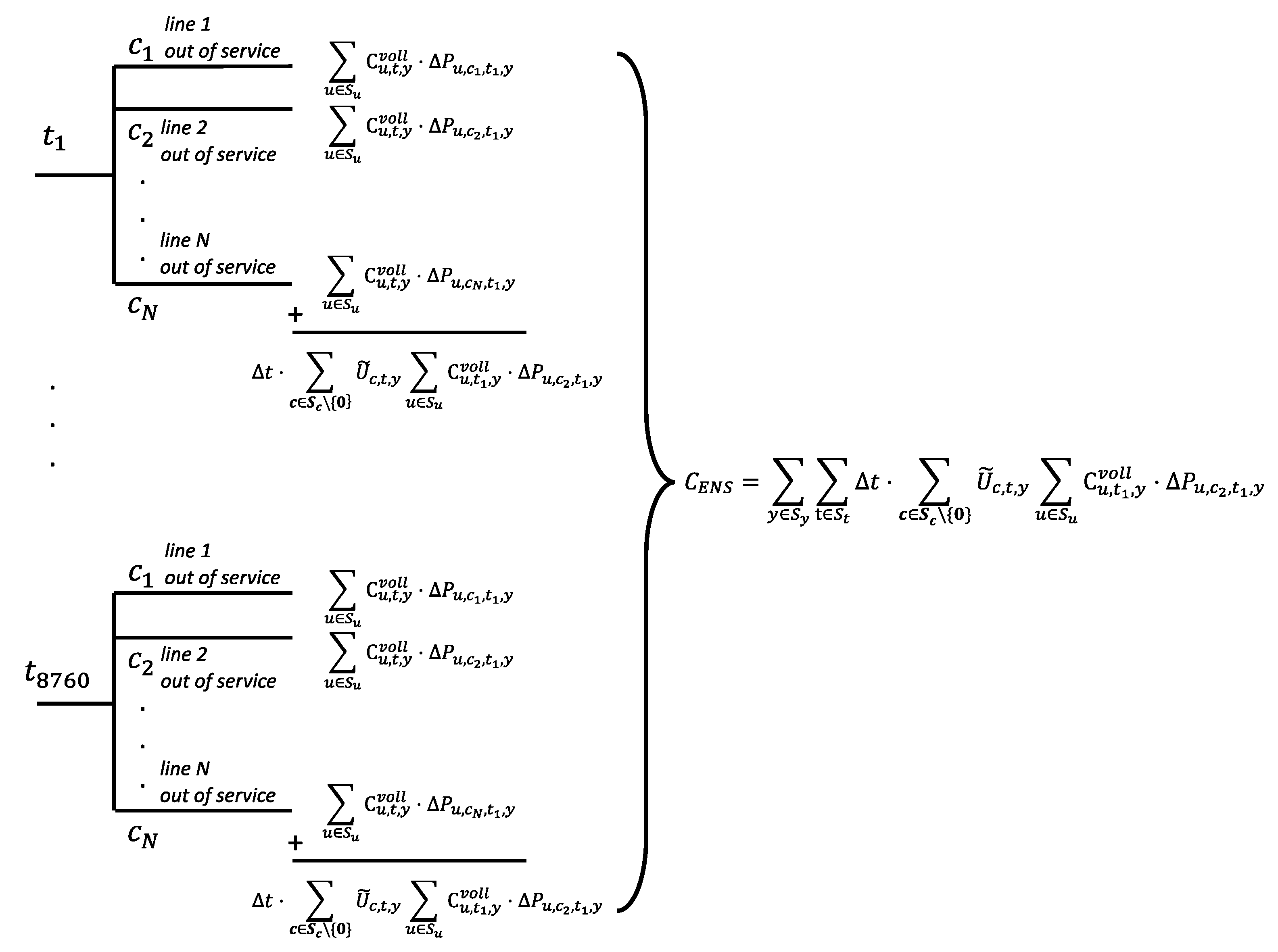
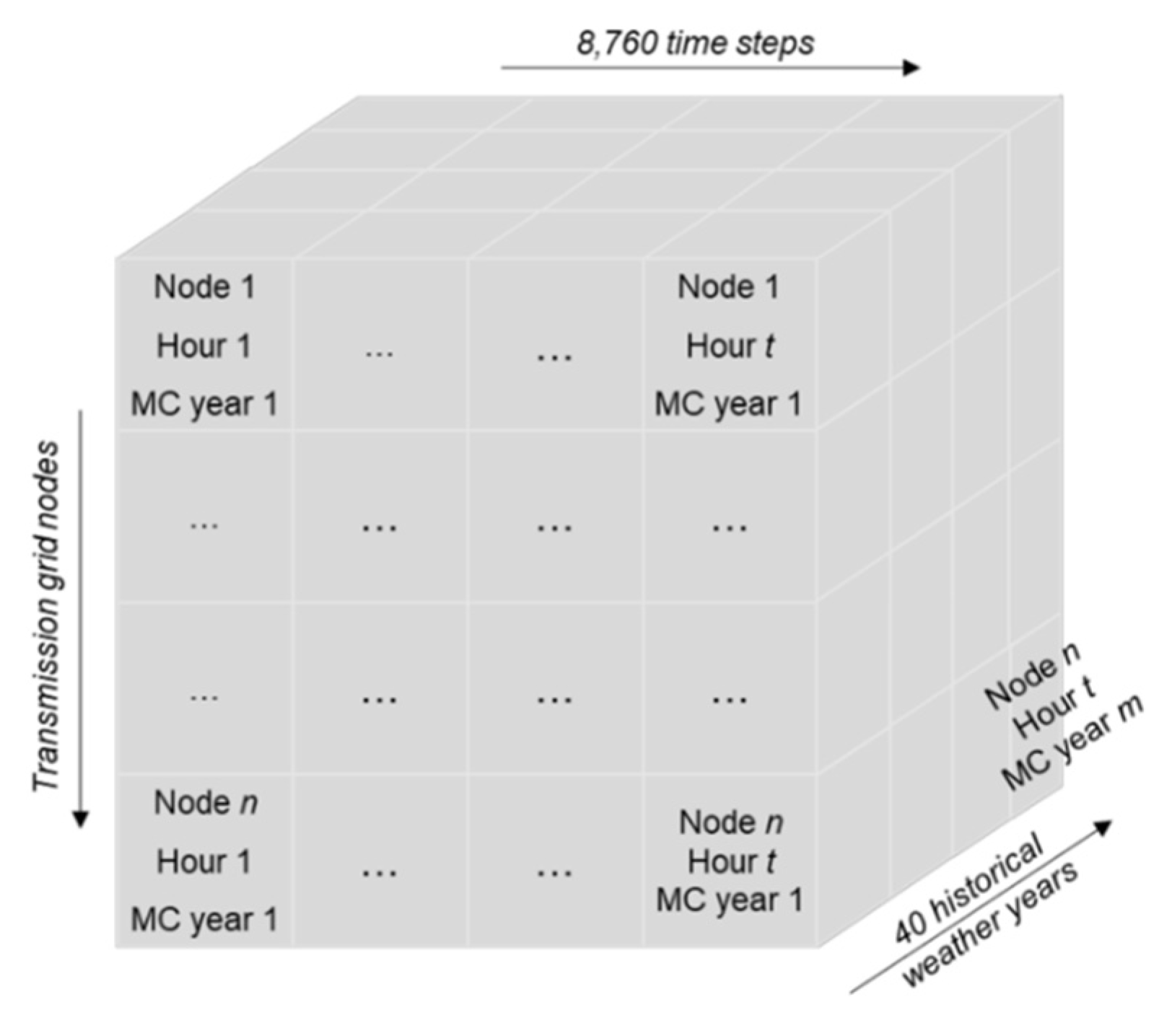
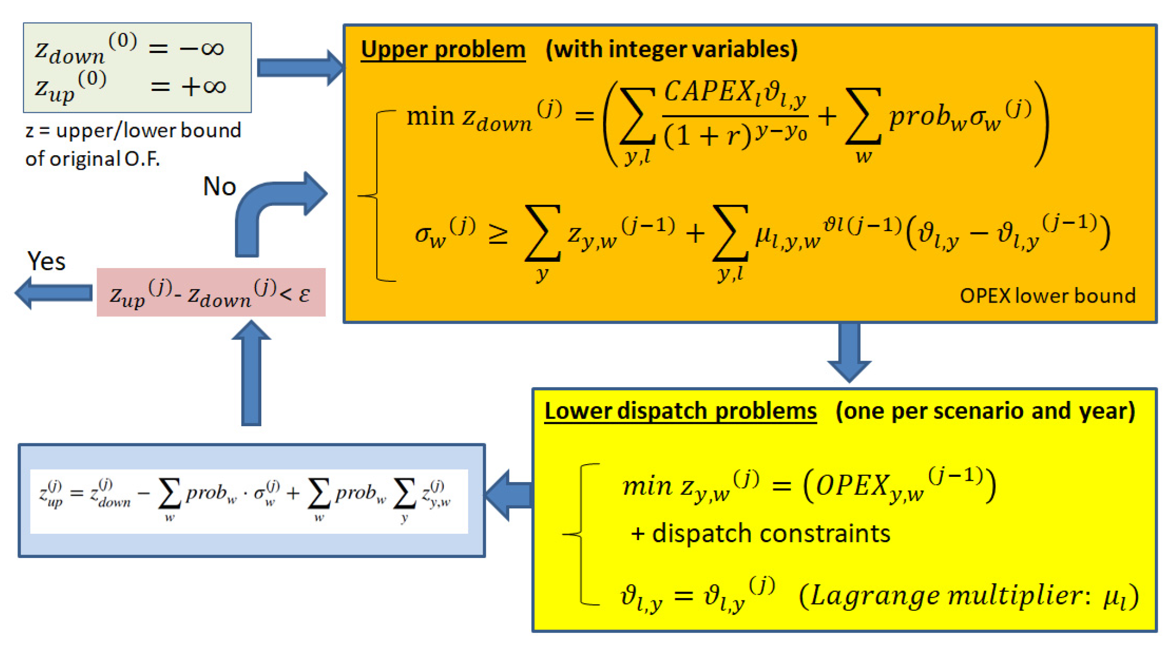
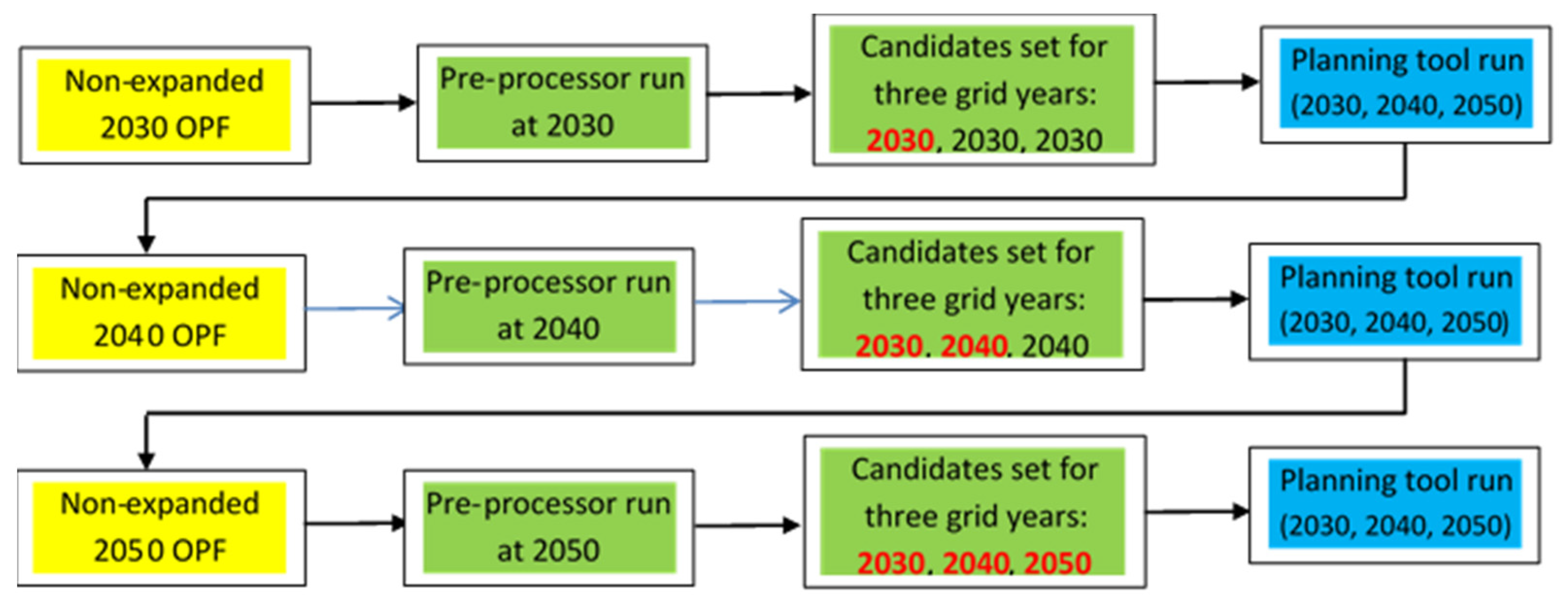
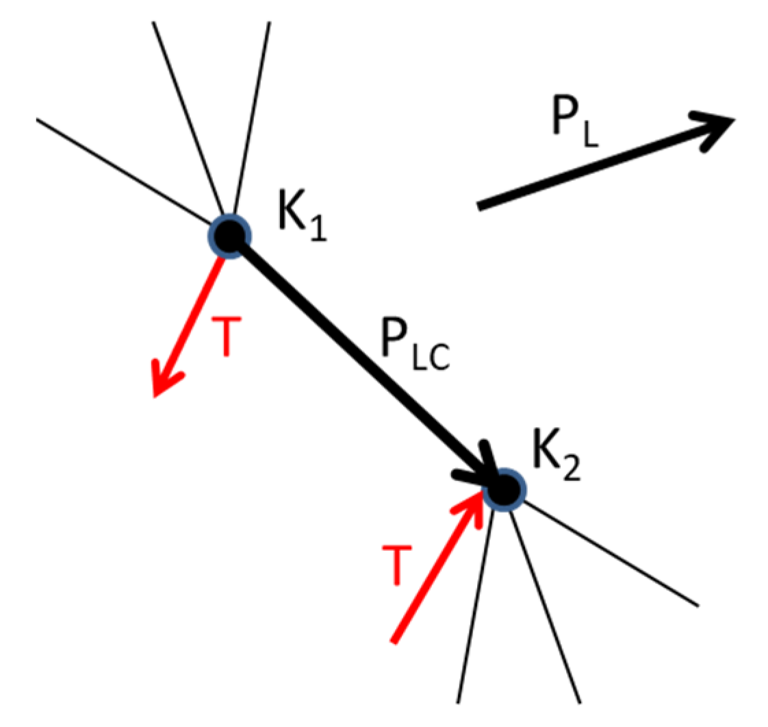
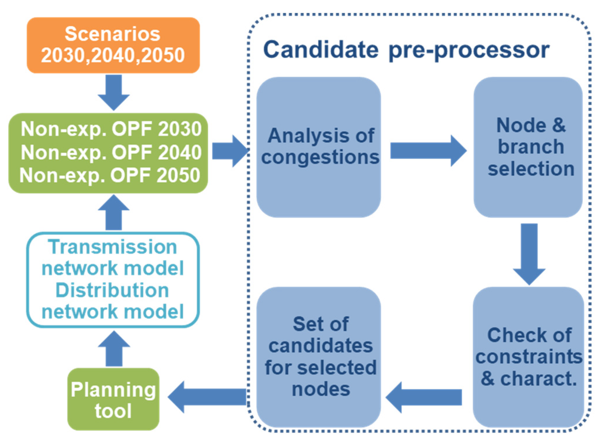
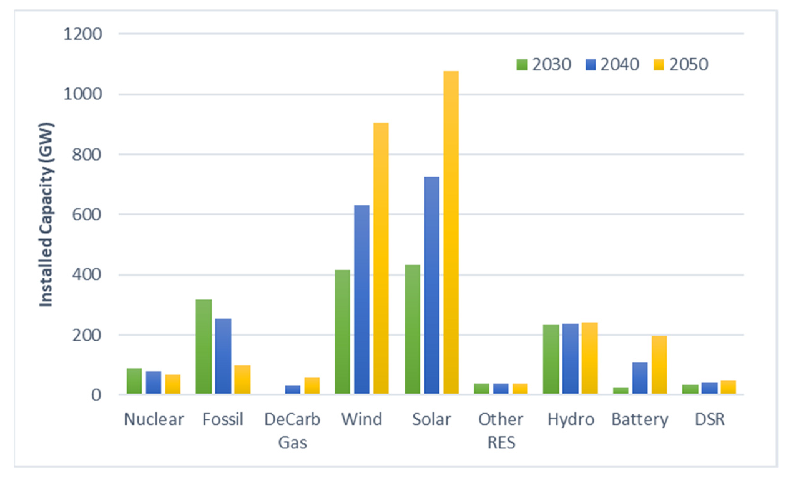
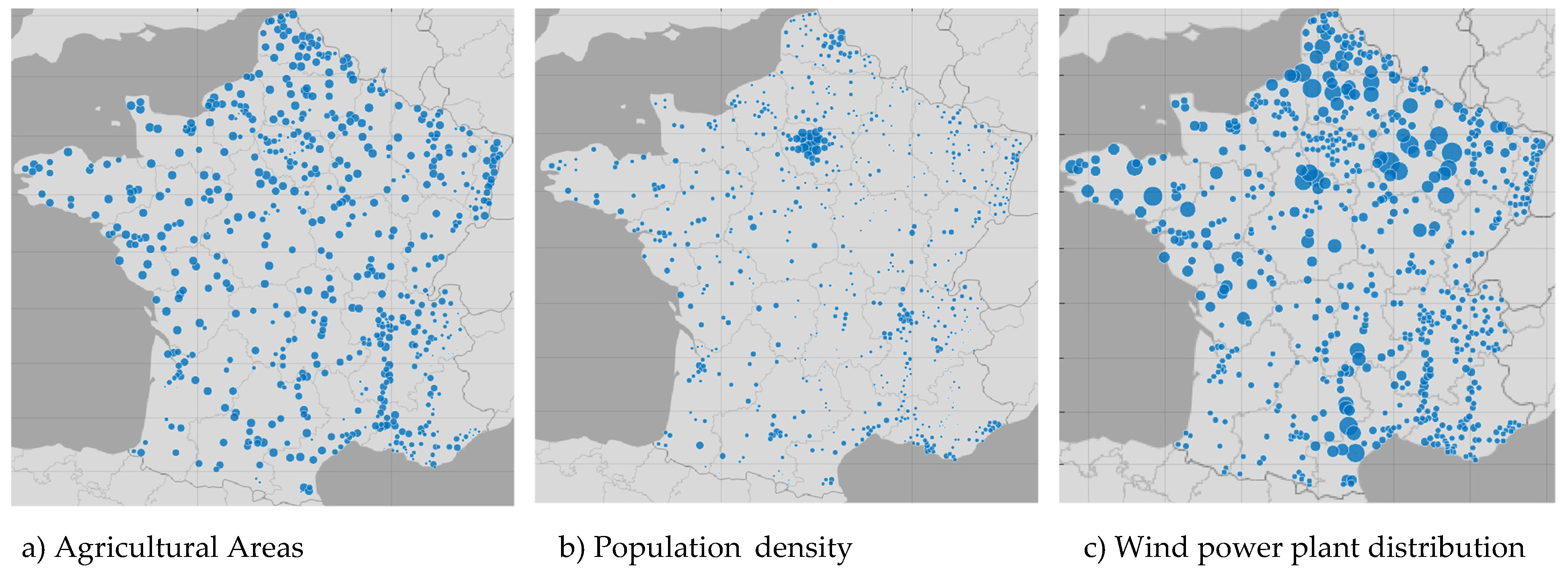
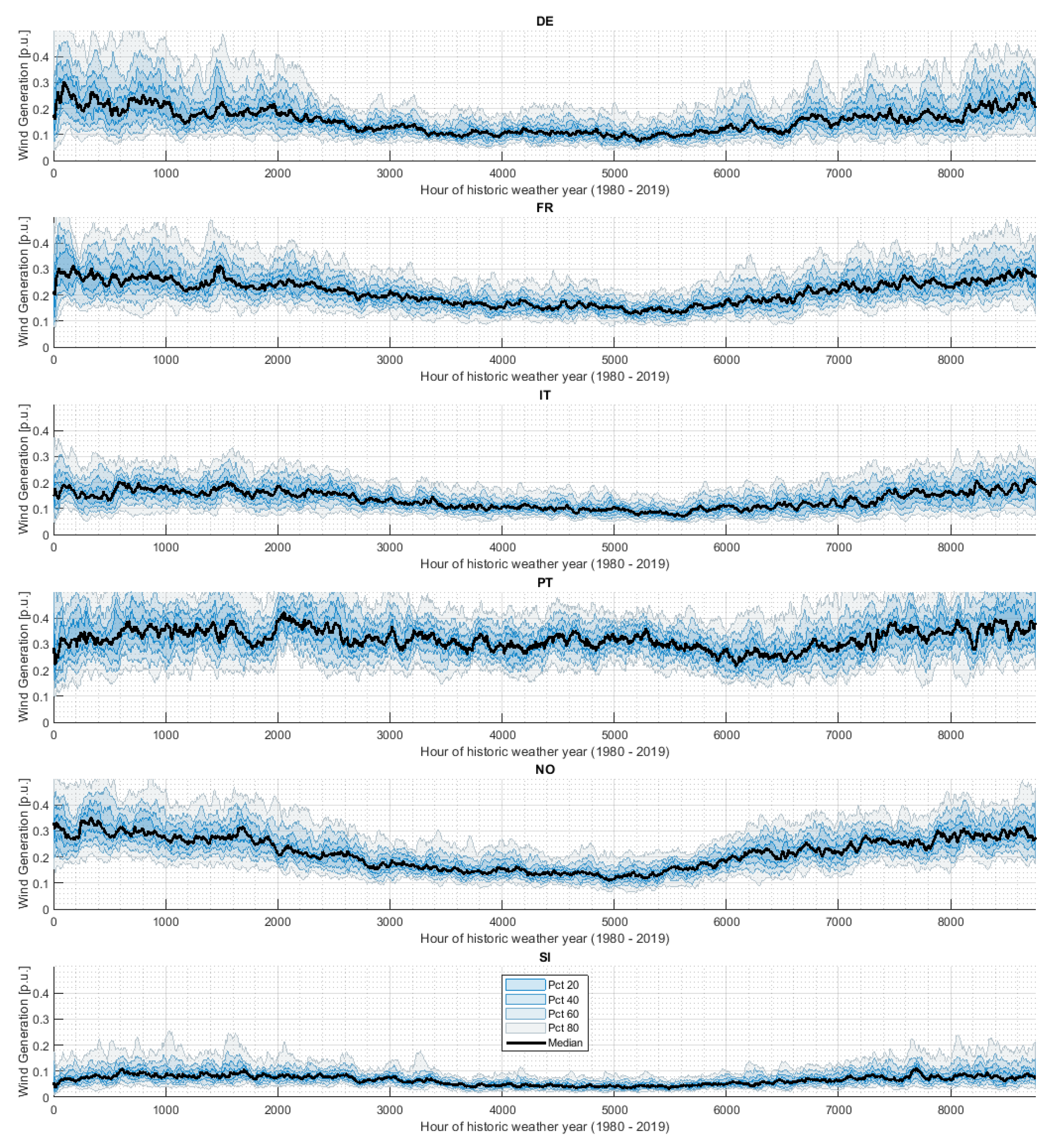
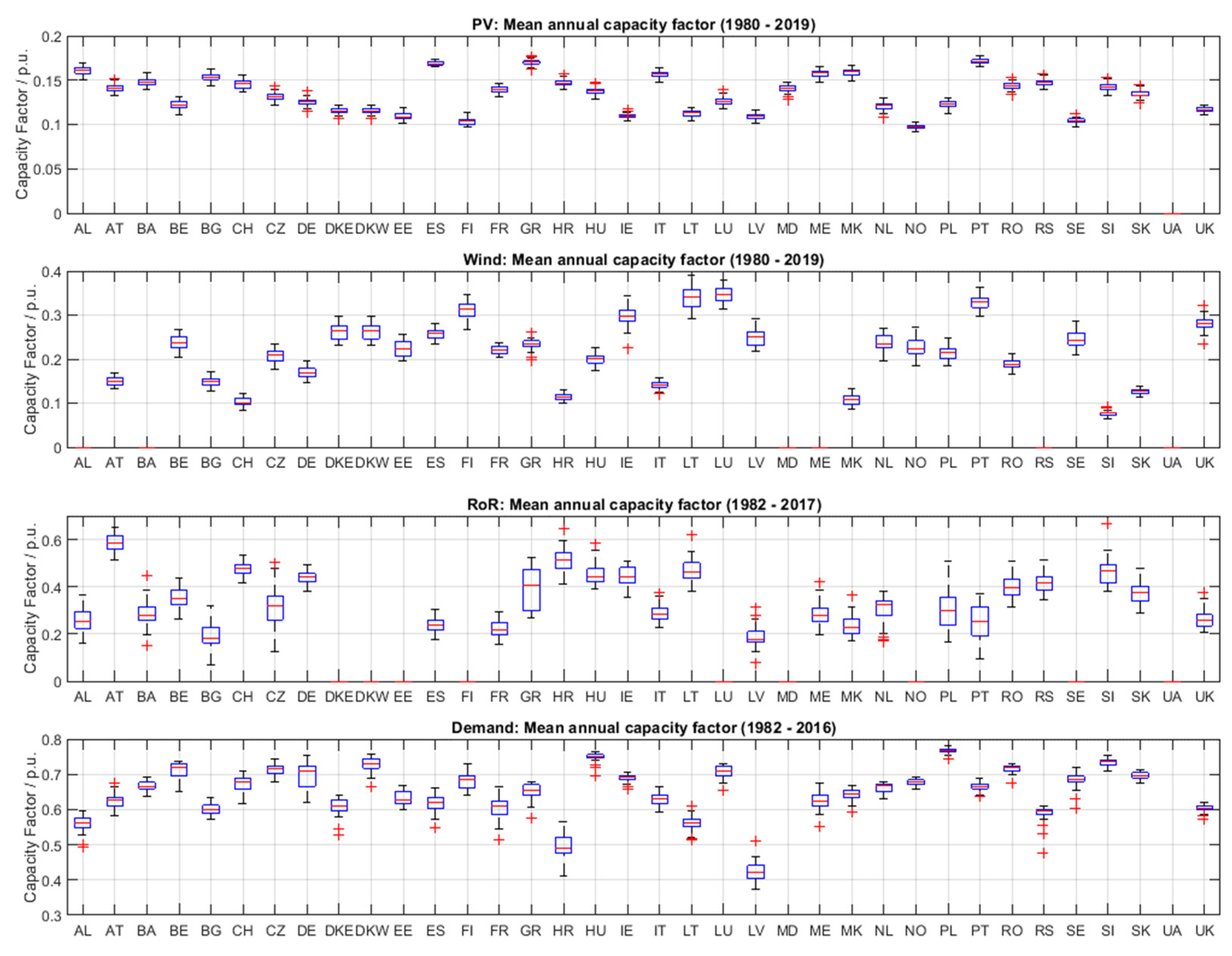
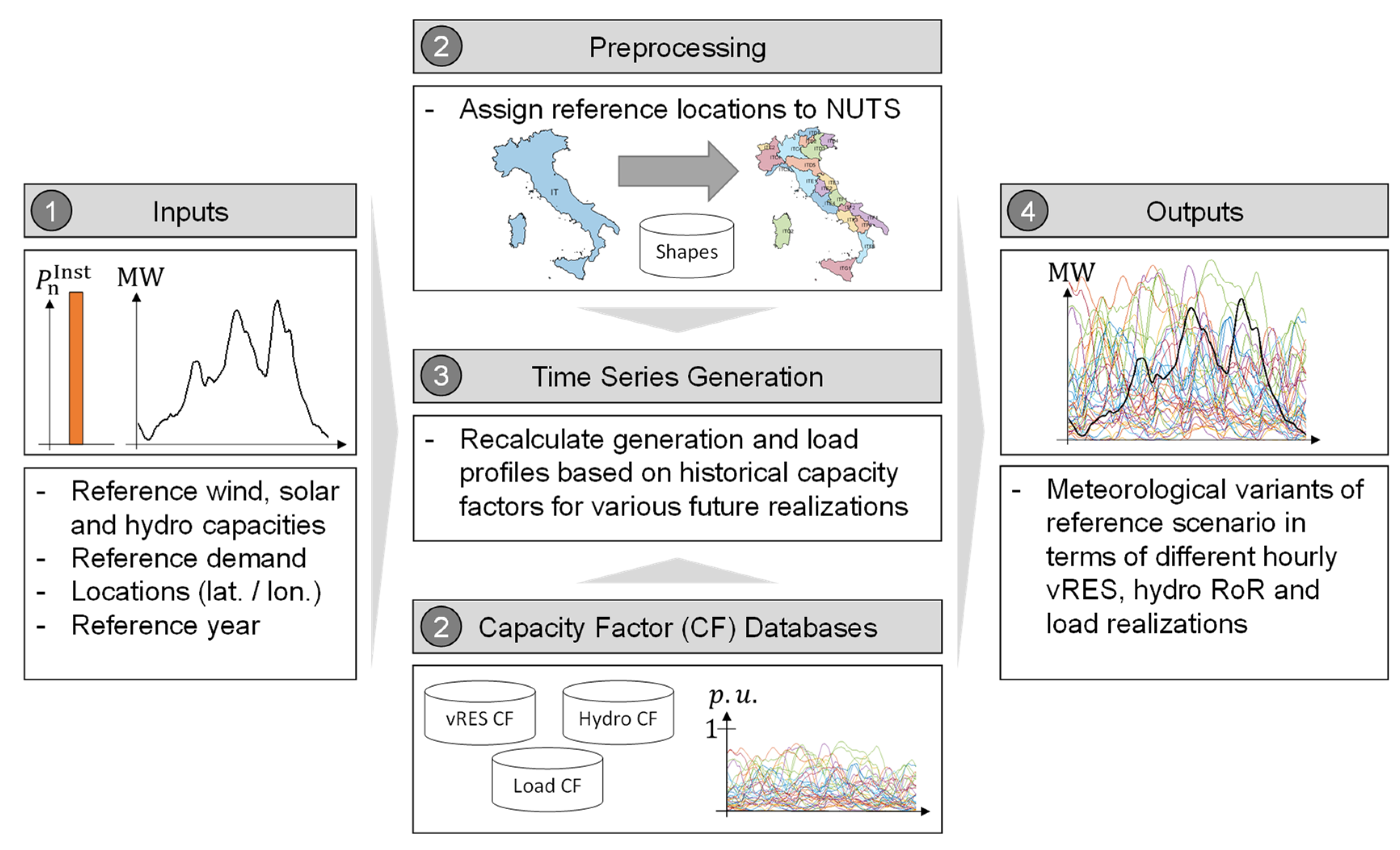
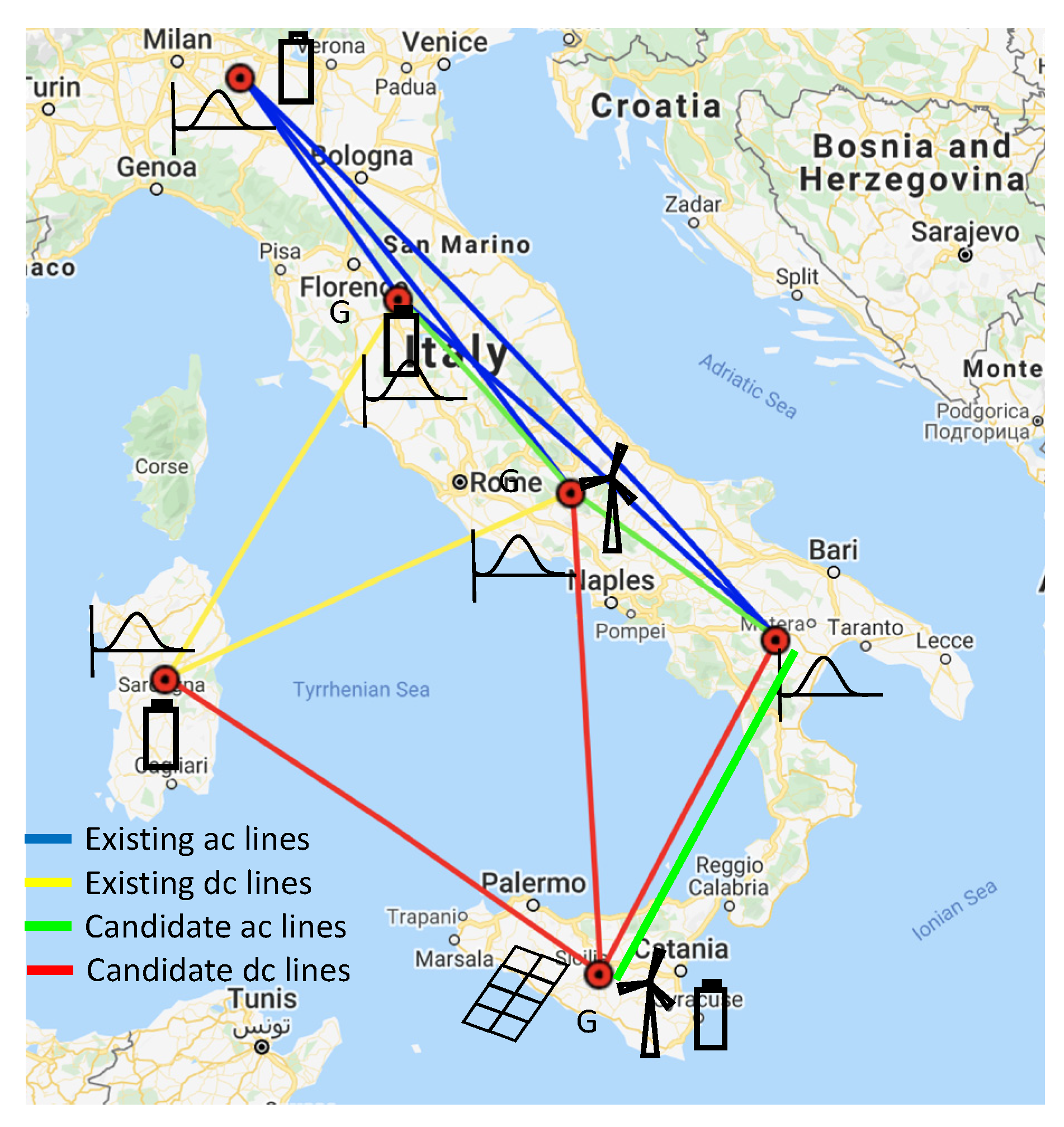
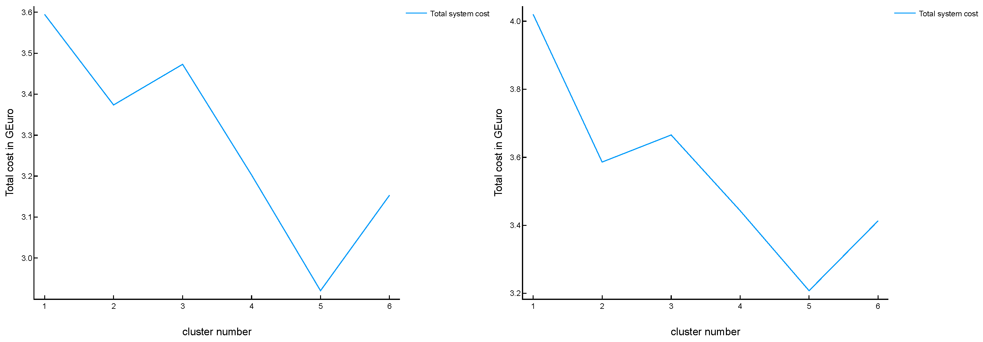
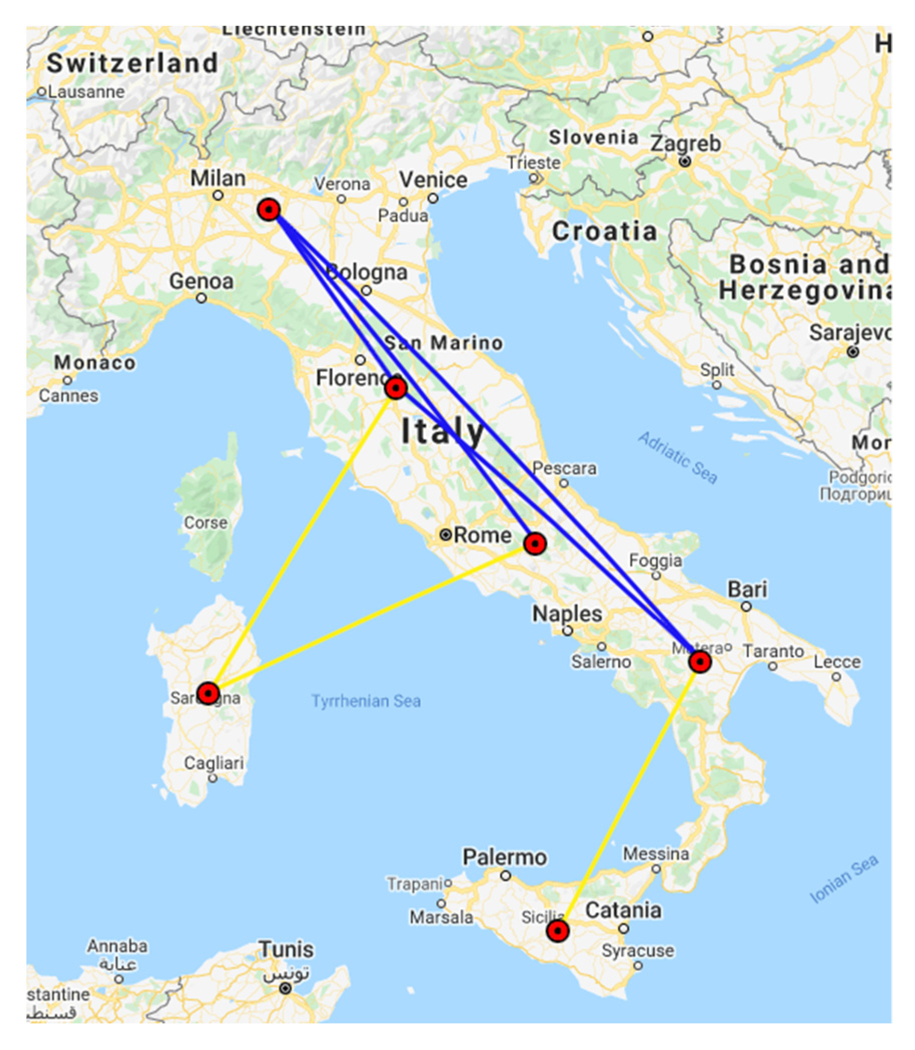