
Particulate Modeling of Sand Production Using Coupled DEM-LBM


Department of Civil Engineering, Engineering Faculty, Ferdowsi University of Mashhad, Mashhad 9177943330, Razvi Khorasan Province, Iran
*
Author to whom correspondence should be addressed.
†
Siavash Honari graduated in Civil Engineering in 2011 and received his M.Sc. in Geotechnical Engineering in 2013 from Ferdowsi University of Mashhad, Iran. He is currently a Ph.D. candidate in Geotechnical Engineering at Ferdowsi University of Mashhad. His research interests include particulate modeling of granular materials and cemented soils using the Discrete Element Method and implementation of the CFD-DEM method to model fluid-solid interactions in porous media, soil erosion, and sand production problems.
Energies 2021, 14(4), 906; https://0-doi-org.brum.beds.ac.uk/10.3390/en14040906
Submission received: 7 January 2021
/
Revised: 29 January 2021
/
Accepted: 30 January 2021
/
Published: 9 February 2021
(This article belongs to the Special Issue Petroleum Geomechanics)
Abstract
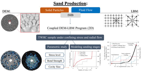
:Sand production is a complex phenomenon caused by the erosion of borehole walls during the extraction of hydrocarbons. In this paper, the sanding process in a typical Thick-Walled Hollow Cylinder (TWHC) test is numerically simulated. The main objective of the study is to model the particulate mechanism of sand production in granular assemblies with different bonding conditions and examine the effects of parameters such as stress level and cavity size on the sanding model. Due to the discrete nature of sand particles, the Discrete Element Method (DEM) is chosen to model solid particles, and the Lattice-Boltzmann Method (LBM) is implemented to simulate fluid flow through the solid particulate medium. A computer program is developed using the Immersed Moving Boundary (IMB) approach to couple the two methods and model fluid–solid interactions. After the program is validated, the simulations were conducted on 2D models representing cross-sections of TWHC samples under radial fluid flow. The results show that the developed program is able to capture complicated stages of sand production already observed in experiments. The program also proves to be a promising tool in the parametric study of sand production. It successfully simulates different aspects of the sanding phenomenon, including the scale effect, the extension of failure zones in samples under incremental stress, and the stress relaxation during rapid particle erosion.
1. Introduction
Sand production, also known as sanding, is an undesirable complex phenomenon [1] affecting the oil industry worldwide. It can be summarized as the separation and erosion of grain particles from the wellbore wall, along with the extraction of hydrocarbons. Redistribution of in-situ stress or the increased effective stress (in a depleting reservoir) leads to the failure of weak rock around the wellbore [2,3,4,5,6]. Consequently, some parts of the rock are disintegrated and may dislocate and enter the extraction well as a result of flow-induced hydrodynamic forces. Unconsolidated or weakly-consolidated sandstones, which comprise almost 70% of the oil and gas reserves, are susceptible to sand production [7,8,9,10]. In addition to causing damage to equipment and facilities [11], sand production also threatens the wellbore stability or might even lead to formation collapse [12,13]. Thus, it is necessary to expand our understanding of sand production and its key parameters to deal with this problem and limit its adverse effects efficiently [14,15,16].
Many experimental studies have been conducted to investigate the sand production mechanism. Regarding unconsolidated sands, primary sand production studies associated the onset of the sand production process with the instability of the sand arch formed near the extraction hole [17,18]. Tippie and Kohlhaas [19] conducted a laboratory study on the effect of flow rate on the arch formation and concluded that the sand arch formation is dependent on fluid flow rate and initial arch size. They also found a new stable (and commonly larger) arch is usually formed after the initial sand arch instability due to excessive flowrate. Yim et al. [20] investigated the effect of fluid pressure, outlet size, and shape of sand particles on the stability of the sand arch. They reported that parameters such as the ratio of grain diameters to cavity size, grain size distribution, and the sand particles’ angularity have a significant effect on the stability of the sand arches.
To study sand production in weakly-consolidated sandstones, Tronvoll et al. [21,22,23,24,25] conducted a series of experimental-numerical studies on the stability of the cylindrical cavities. Thick-Walled Hollow Cylinder (TWHC) samples were used in the experiments to mimic field sandstone around boreholes. They found that although mechanical instability is mainly responsible for sand production, the role of hydromechanical instability and fluid flow increases as the strength of sandstone decreases, and the sanding behavior gets more complicated for ultra-weak samples. They also reported that the sand initiation strongly relies on the Uniaxial Compressive Strength (UCS) of the samples, while it is independent of fluid flow conditions. In a similar study, Papamichos et al. [26] explored the effects of stress level and fluid flow on sand production in weak sandstones and found that increased applied stress leads to higher sanding rate and more produced sand. Papamichos [27,28] conducted further studies on the effect of perforation size, sample strength, and stress anisotropy on sand production. He reported that the cavity enlargement decreases the sand initiation stress, whereas stronger samples show higher sand initiation stress. Similar parameters were studied by Fattahpour et al. [2,3]. They recognized five distinct sand production stages in their experiments, including sand initiation, transient, semi-continuous, continuous, and catastrophic sand production. According to Fattahpour et al. [2], the stress level is responsible for each sanding stage, and as the stress level increases, higher sand volumes are produced. They also reported that stronger rocks are more sensitive to cavity enlargement than weaker ones. To study the effect of stress conditions and fluid flow on sanding, Younessi et al. [29] conducted a series of sand production tests using a true-triaxial stress cell. They argued that the shape of failure zones around the borehole is a function of stress anisotropy. They also observed that the sandstone yield occurs prior to the onset of sand production, and with the increase of stress level, the amount of produced sand and the yield zone dimensions around the borehole increase.
The experimental studies of sand production face some difficulties that restrict their application. The limited dimensions of laboratory equipment and the subsequent small samples usually used in experiments might affect the accuracy of test results [29]. Experiments using larger samples are expensive and more challenging to implement [15]. Numerical simulation is a cost-effective alternative for laboratory experiments to study sand production [13]. Due to the particulate mechanism of the sand production process, the Discrete Element Method (DEM) is a suitable approach to model the sanding phenomenon. In these models it is essential to accurately incorporate the impact of fluid flow into the interaction of solid elements modeled in DEM formulations [14].
A continuum-discrete approach was used in the first attempts for the DEM-based simulation of sand production [30,31,32,33,34,35]. In this approach, solid particles are modeled using DEM, yet the fluid is considered a continuum whose behavior depends on macroscopic parameters such as permeability through semi-empirical Equations. More recently, Climent et al. [36] developed a 3D model to study the effect of fluid flow and in situ stresses on the sanding process with limited stress and fluid conditions. They observed that the hydrostatic fluid (at the no-flow condition) reduces the amount of produced sand as it acts as a damper decelerating the eroding particles. A similar study was conducted by Cui et al. [37], where special attention was paid to the evolution of porosity and permeability in the porous media.
Following the pioneering works of Cook et al. [38,39], many researchers have used a fully discrete approach to numerically study sand production with more accuracy [1,40,41]. In this approach, both solid and fluid phases are treated as discrete particles, and consequently, the results are independent of macro parameters such as permeability. Similar to Cook et al. [39], Han and Cundall [41] employed the Immersed Moving Boundary (IMB) method (which will be explained in Section 2.3.1) to couple the Lattice-Boltzmann Method (LBM) with DEM. They modeled the stabilization and collapse of sand arches in a perforation cavity subjected to various fluid pressures, trying to simulate the episodic sand production of unbonded particles in 2D. Their results showed that the expected collapse and reformation of sand arches near the cavity could be qualitatively captured using coupled DEM-LBM. In another study, Wang et al. [1] investigated transient sand production using a similar approach with cemented particles. Bond models were used to simulate the cementation between particles. They could successfully model the enlargement of the tensile failed zone around the wellbore cavity and the erosion of particles in this zone due to fluid drag forces.
Although sand production has been studied extensively, the complexity and the importance of this phenomenon calls for more research. The main goal of this study is to simulate the sanding mechanism of a conventional TWHC test in 2D and to simulate the model’s loading and fluid conditions similar to the ones present in the TWHC samples. Special attention is paid to explore the interaction between the key parameters in sand production and to capture the different stages of this process previously found in experimental results. For this purpose, a cross-section of the hollow cylinder, in the form of a ring-shaped porous medium, is modeled while subjected to radial flow. Full-sized samples are modeled to prevent the disruption of radial flow and acknowledge that the DEM medium is not perfectly homogenous [36,37]. Since the particulate nature of sand production has significant responsibility in its complication, solid particles in the current study are modeled using DEM. To accurately capture the dynamics of the fluid flowing through particulate porous media, LBM is chosen as the fluid solver. The IMB method, proven to be reliable by previous studies [1,41], is chosen to couple the two numerical approaches and model the fluid–solid interaction. An in-house computer program is developed to simulate sand production in both unconsolidated and weakly-consolidated media, in which a simple bond model reproduces the effect of cementitious materials. In the developed program, the solid particles are modeled as polygons with arbitrary shape, enabling the program to consider various (thus more realistic) shapes for solid particles. However, particle shape in the sand production process is not studied in this paper and will be tackled in future research. After the program validation using multiple benchmark and qualitative tests, the sand production simulations are finally undertaken, including a series of parametric studies.
As mentioned, the novelty of the study mostly lies in the improvements applied to the numerical modeling of sand production, including (a) particulate modeling of both solid and fluid phases (to capture the complicated mechanics of the sandstone and eliminate the use of complex parameters such as permeability), (b) modeling full-sized ring-shaped samples (in contrast to half-sized or wedge-shaped ones), (c) modeling radial flow (similar to the actual fluid flow direction in the TWHC test), (d) considering the effect of inter-particle cementation (to enable the developed program to study sand production in weakly-consolidated sandstones as well as unconsolidated ones), and (e) using angular shapes for solid particles (to resemble the increased interlocking of actual irregular-shaped sand particles).
This paper is organized into five sections. After introducing the problem in this section, the methodology and the basis of the approaches used in the current study are provided in Section 2. In Section 3, the developed program is validated through diverse benchmark tests. After that, Section 4 covers the modeling procedure and the results of the sand production simulations. The results confer the model’s capability to capture different stages of sand production. They cover the effect of multiple parameters on sanding results, including stress level, bond strength, and cavity size, compared with the published experimental data. Finally, Section 5 is devoted to draw the main conclusions and suggest topics for future studies.
2. Methodology
2.1. Bonded Discrete Element Method
Discrete Element Method (DEM) was first introduced in 1971 [42] to model the behavior of distinct particles in granular environments. In this method, a set of sequential cycles must be performed at time-steps to track particles’ movements and mechanical interaction over time. At each time-step, after finding the particles in contact, the inter-particle interaction is modeled by force-displacement relations at each contact. Then, for each particle, total forces and moments are calculated, and after that, the particles’ movement and rotation are updated using Newton’s second law.
In the current study, an in-house computer program called “BDL2D” was developed to conduct simulations using coupled DEM-LBM on bonded particle assemblies. The DEM module of the program is originated from the computer code “POLY” introduced by Mirghasemi et al. [43] to simulate the mechanical behavior of granular assemblies using polygonal particles. The DEM module was modified in the current computer program so that it can model inter-particle bonds to mimic the effect of cementation between particles. Same as the original code, “BDL2D” uses linear contact law as described by Mirghasemi et al. [43]. Other instances of the development and application of the original code are the simulation of particle breakage [44,45], the effect of inherent/induced anisotropy on the behavior of granular materials [46,47,48,49], and instability of saturated granular materials [50].
The inter-particle bond in the current computer program, in essence, is a modified contact model between initially contacting particles (at the instant of bond creation). A relatively simple bond model similar to the approach originally proposed by Jiang et al. [51] was used. It is found that this model can efficiently capture the primary mechanical behavior of bonded particles [52,53]. The model adds a bond element into the existing contact model with only tensile and shear resistances. The rolling resistance of bonds is neglected since its value is arguably negligible if the size of the bonds is small enough compared to the particle size [51]. The bonds break irrecoverably once the tensile or shear forces exceed the corresponding strength of the bonds. When in tension, the bond provides an attractive contact force primarily equal to the product of normal stiffness and normal displacement, reaching the tensile bond strength, , at its peak value. Once the bond is broken due to excessive tension, the attractive contact force abruptly drops from to zero. The shear bond contact model behaves somewhat differently. The contact shear force increases linearly with the shear displacement until its peak value, . In the case of shear bond breakage because of excessive shear force, the strength of the contact abruptly drops to the residual frictional strength (defined by the Mohr–Coulomb criterion). The approach is explained in detail by Jiang et al. [51,52]. It is befitting to note that in the current study, for simplicity, the normal and shear bond strength values were assumed to be equal ().
2.2. LBM
The Lattice-Boltzmann Method (LBM) is a simplified numerical solver for Computational Fluid Dynamics (CFD), simulating fluid flows using a particulate approach. The time-step computational mechanism of LBM makes this approach a suitable coupling match for DEM. Furthermore, the particulate nature of LBM enables it to incorporate complicated solid boundaries more easily. Even compared to other particle-based fluid solvers (such as smoothed particle hydrodynamics [54]), LBM is more mature in dealing with complex boundaries [55]. This advantage makes LBM an attractive approach for accurately modeling fluid flow through porous media [56] as the fluid “naturally” flows through the medium pores [57], without a need for complicated parameters such as permeability of the porous medium.
In LBM, the fluid flow is divided into fictitious particles forming a uniform square-shaped grid. The flow propagates through the grid, one node at a time-step and collides with other flow particles along the way. These “streaming” and “collision” steps simulate the macroscopic behavior of the fluid flow. In general, the virtual fluid particles have infinite degrees of freedom. However, for simplification, a reduced number of degrees of freedom is considered and the particle momentum is discretized. It means that the emission of these particles occurs only in specific directions regarding the regular square grid network. Figure 1 shows an example of lattice network and the unit velocity vectors () for each node in this network, representing the degrees of freedom of the fluid particles. This figure is related to a nine-speed network in two dimensions, called D2Q9, a commonly used velocity set in 2D models.
As shown in Figure 1, is “lattice spacing”, the uniform size of the lattice cells throughout the fluid model. The discrete-velocity distribution function , often called the “particle populations”, represents the density of particles with the same velocity at position and time . In essence, the particle population is the proportion of fluid particles in a lattice node, moving along the ith direction of the node [58]. Accordingly, the macroscopic fluid density () can be calculated as:
The LB equation can be formulated as:
in which, is the LBM time-step. According to Equation (2), particles of move with unit velocity to an adjacent point at the next time-step (). During this propagation, the particles are also affected by the collision operator , which models the particle collisions by redistributing particles among the populations at each site [58]. There are many different collision operators and the simplest yet most well-known one is introduced by Bhatnagar, Gross, and Krook [56], abbreviated to BGK. This operator uses a single relaxation time, which basically means that it relaxes the populations toward the equilibrium distribution at a rate determined by the relaxation time . Equation (3) shows the BGK collision operator:
After combining Equations (2) and (3), the LB equation with single-relaxation-time approximation can be expressed as:
The equilibrium distribution function is a function of the direction index () and can be represented as:
where are the weighting factors specific to the chosen velocity set. For the D2Q9 velocity set used in this study, are defined as:
and is the lattice speed, defined as . The fluid velocity , used in Equation (5), can be calculated as:
To calculate the fluid pressure at any fluid node, Equation (8) can be used:
where is the speed of sound in fluid and can be calculated based on the lattice speed as: . Kinematic viscosity is another macroscopic quantity of the fluid and can be formulated as:
The LBM originally treats the fluid as weakly compressible [58]. Equation (8) clearly shows that a pressure difference between two fluid nodes is originated from a density difference between them. However, a suitable parameter selection for the LBM model would limit the so-called compressibility errors. To be more precise, if the computational Mach number is kept small enough (), the error is negligible. Practically, a fluid flow with is assumed to be incompressible [59]. The computational Mach number in LBM models can be calculated as [60,61]:
where is the maximum fluid velocity throughout the model. In the present study, great attention was paid to the value of the Mach number to satisfy the previous fluid compressibility limit in all coupled models.
2.3. DEM-LBM Coupling Scheme
As already mentioned, the accuracy of particulate models of sand production highly depends on the proper incorporation of fluid–solid interaction. Therefore, it is necessary to apply the flow-induced drag force to the motion calculation of solid particles and, in turn, consider the effect of particle motion on the behavior of fluid flow [37]. To conduct this “coupled” scheme, one needs to accurately: (1) Identify the fluid–solid interfaces and (2) calculate the hydrodynamic forces and moments acting on the particles. Once these values are calculated, they are exported to the DEM module as fluid-induced input data. Then, they are added to solid contact forces, and after that, the combined forces and moments lead to the determination of the new position of solid particles.
When moving solid objects exist in the model, especially with high-velocity, the hydrodynamic forces computed from the simple bounce-back rule (explained in [58]) suffer from severe oscillations. To deal with this problem, researchers proposed more advanced coupling schemes, such as the Immersed Boundary Method (IBM) and the Immersed Moving Boundary (IMB) method. One should pay attention to the difference between the IBM and the IMB method as the former is proposed by Peskin in 1977 [62], while Noble and Torczynski introduced the latter in 1998 [63]. The IMB method is sometimes called the Partially Saturated Method (PSM) to avoid confusion [64]. Wang et al. [60] made a thorough comparison between IBM and IMB. They concluded that while the two approaches lead to similar results in some cases, IMB is substantially more accurate when fluid velocity or particle movement is large (e.g., when sand production is modeled). They also reported that IMB is more computationally efficient than IBM. In the following section, the IMB method used in the current study is explained in detail.
2.3.1. Immersed Moving Boundary (IMB) Method
The IMB method uses a modified LB equation. In this method, the standard collision operator of LBM is altered by adding an additional collision term, . This new term is used to approximate the complex solid boundaries on lattice nodes so that the boundaries of solid particles are smoothly represented in the regular grid network. This representation is characterized based on a parameter called solid ratio, introduced for each computational lattice cell as shown in Figure 2. This parameter is defined as the area occupied by a solid phase, (the hatched area in Figure 2), to the total cell area ().
The modified LB equation is given by [63]:
where B is a weighting function depending on the local solid ratio parameter:
According to Equation (12), for a pure fluid node, and . On the contrary, at its peak, for a pure solid node, and then B = 1. The additional collision term is given by Cook [38] as:
where subscript denotes the opposite direction of , is the local fluid velocity, and is the velocity of the particle at each solid node, evaluated as a combination of transition and rotation [61]. Finally, total hydrodynamic forces and moment exerted on a solid particle which is mapped over lattice nodes can be respectively computed as:
where and are the coordinates of lattice node n and the mass center of the solid particle, respectively.
In 2D models of fluid flow through dense particulate media, there is a major issue regarding the pore water flow path. In these conditions, the flow paths are blocked by contacted solid particles, making it difficult for fluid to flow through the media. The hydraulic radius concept was introduced to numerically solve this problem and facilitate fluid flow through adjacent particles in the 2D DEM-LBM models [35]. The hydraulic radius is the virtual radius of a particle in the LBM calculations, smaller than the mechanical (real) radius of the particle. The hydraulic radius multiplier is defined as the ratio of the hydraulic radius to the real particle radius. It should be noted that the hydraulic radius is only applied in LBM (fluid-part) calculations, and the DEM (solid-part) model uses the mechanical (real) radius of the particle [1,40,65,66].
2.3.2. Subcycling Time Integration
Since the LBM time-step is greater than that of DEM in the simulations, subcycling time integration is used to couple the two methods. As proposed by Owen et al. [61], the authors reduced the DEM time-step so that the LBM time-step is an integer product of it:
where , , , and are the time-steps’ ratio rounded up to the nearest integer, initial DEM time-step, final (reduced) DEM time-step, and the LBM time-step, respectively. In the subcycling approach, each LBM cycle includes some DEM cycles during which the hydrodynamic forces and moments remain unchanged. It is suggested that should be limited to small values [59] so that the LBM calculation ideally updates before solid boundaries cross through more than one lattice cell [61]. In the simulations in the current study, the subcycling scheme led to promising results where Nsub < 10.
3. Model Validation
Having developed the computer program based on the described computational methodology, the authors conducted a series of tests covering various aspects of the program. The purpose of these tests is to validate the program and to examine its accuracy in each area.
3.1. Poisseuile Flow
One of the most famous benchmark tests for CFD modeling is Poiseuille channel flow. It considers the steady laminar flow between two parallel plates, from inlet to outlet, perpendicular to the plates. Poiseuille flow can be driven by velocity, pressure difference (gradient), or body force (such as gravity). The parallel plates are wall boundaries enforcing a so called “no-slip” boundary condition at their interface with the fluid. Thus, the fluid velocity at the walls is zero while it reaches its maximum in the middle of the channel. Besides simplicity, the popularity of Poiseuille flow as a CFD validation tool is mostly because it has a closed-form solution. As illustrated in Figure 3, the parabolic velocity profile for a pressure-driven Poiseuille flow is given by [56]:
where , , , and are the pressure gradient, fluid density, fluid kinematic viscosity, and channel width, respectively.
Here, a pressure-driven Poiseuille channel flow (as shown in Figure 3) with the parameters listed in Table 1 is modeled, and the results are compared with the analytical results from Equation (18). Note that the value of pressure difference is opted to result in a Reynolds number of 1.
The horizontal velocity of fluid across the channel is computed for three different lattice spacings using the developed code, and the results are compared with analytical values in Figure 4. The relative error in calculating maximum fluid velocity (in the centerline of the channel, i.e., ) is 9.61%, 3.77%, and 0.23% for 5, 2, and 1 mm, respectively. Thus, as expected, the finer the lattice mesh, the closer the numerical results to the analytical ones [41]. The results show that fluid behavior (in the absence of solid particles) is accurately simulated in the developed code, especially when mm.
3.2. Single Particle Sedimentation
The sedimentation of a circular particle in a confined channel has been studied as a validation case for many numerical methods. Hu et al. [67] and Wu and Shu [68] studied this problem using an arbitrary Lagrangian–Eulerian finite element method and implicit IBM-LBM, respectively. Wu et al. [69] also modeled the same problem using coupled DEM-LBM with multiple boundary schemes, including the IMB method.
A similar problem, the sedimentation process of a single solid particle in a fluid-filled vertical container under its gravity is simulated using the developed program, and the results are compared with the studies mentioned earlier. The geometry of the container and the initial location of the particle is demonstrated in Figure 5. All four boundaries of the square-shaped container are no-slip walls imposing the simple bounce-back rule to the fluid particles. Similar characteristics are considered for the model to maintain comparability with the previous studies. The fluid density, kinematic viscosity, and particle density are 1000 kg/m3, m2/s, and 1250 kg/m3, respectively. A lattice spacing of h = 0.1 mm is used and the relaxation time is set to τ = 0.65. As the developed computer program (BDL2D) can only model polygon solid particles, a 20-sided regular polygon as a pseudo-circular particle is introduced in the model to resemble the circular one. The reason for using a regular polygon with multiple sides is its geometrical resemblance to a circle. The polygon dimensions were chosen to be inscribed in the corresponding circle with 2.5 mm diameter, same as the settling particle in Wu et al. [69].
Figure 6 shows the results of the sedimentation model for vertical position and velocity of the settling particle compared to the results of previous numerical studies. The current results are in perfect accordance with the previously published data and almost coincide with the results of Wu et al. [69]. According to Figure 6b, the vertical velocity of the settling particle increases until it reaches its terminal velocity at time ~0.4 s and remains constant afterward. Figure 6a supports this perception as the diagram’s slope does not change for time > 0.4 s until the particle reaches the bottom of the container. It can also be inferred that the difference between the geometry of the 20-sided polygon and the circle with the same diameter has a negligible impact on the sedimentation results. It is also approved that while the developed program cannot simulate particles with curved surfaces, the hydromechanical behavior of these particles can be reasonably captured using regular n-sided polygons. It is understandable that the higher the n, the more accurate the results are. At least for simple hydromechanical models (such as single-particle sedimentation), the movement of the circular particle movement can be simulated by using a regular 20-sided polygon.
3.3. Bonding Effects on Particulate Assembly
In this section, to ensure that the developed program can capture the general behavior of bonded granular assemblies, the effect of bond presence between particles is investigated by conducting a series of DEM tests. These tests simulate biaxial experiments on dry specimens with different bonding conditions, carried out in different steps, as graphically shown in Figure 7. These steps are described in detail as follows:
- Particle generation: The desired number of polygon particles are randomly placed in a circular assembly. In this step, the particles have no overlap, and the number of generated particles with each specific size follows the given particle-size distribution.
- Initial compaction: A stress-controlled isotropic compaction is applied on boundary particles. The boundary stress is maintained until the desired planar void ratio is achieved. It might be challenging to form loose homogeneous models with high values of void ratio. Relatively loose models can be formed if high values of inter-particle friction coefficient and considerable damping are considered while small boundary stresses are applied during the initial compaction. Conversely, if dense particle assemblies are to be modeled, negligible damping and zero friction coefficient should be considered.
- Bond generation: If cemented particles are to be simulated in the assembly, bonds are created at all existing contacts at the beginning of this step (as explained in Section 2.1).
- Confining stress: In this step, the particle assembly is subjected to given isotropic boundary stress. The intergranular friction coefficient and damping constants should be restored to common values at the beginning of this step.
- Deviatoric stress: When the variation of the planar void ratio with loading cycles becomes negligible during confinement, the last step of the biaxial test can be initiated. In this step, while maintaining the confining boundary stress of the previous loading step, a compressive displacement is applied vertically at a uniform rate, increasing the vertical stress of the assembly. The test continues until the particle assembly reaches high vertical strains.
In the current biaxial studies, 2000 octagonal (regular eight-sided polygon) particles with relatively uniform sizes are generated. Compared to circular particles used in previous numerical studies, the particles’ octagonal shape can mimic the increased interlocking of actual irregular-shaped sand particles as most of the grains in natural sandstones are angular [3]. On the other hand, the roundness of octagonal particles helps avoid induced anisotropy in the model [46]. The particle diameters range from 3.56 to 2.14 mm. The particle size distribution of the particle assembly is demonstrated in Figure 8. To reduce the number of DEM particles and, therefore, the computation cost, the sand particle sizes in the experimental study of Younessi et al. [29] are magnified by a factor of 5. The planar void ratio of the particle assembly is 0.20 after the initial compaction. The boundary stress at the initial compaction step was 12.5 kPa. The stress was kept constant during the bond generation step when three different bond strengths (50, 500, and 5000 N) were applied to particle contacts of three sets of models. After that, each set of bonded models and unbonded particle assembly were subjected to 50 and 100 kPa isotropic stresses during the confining stress step. Each model is then subjected to deviatoric stress caused by vertical compression, and their stress–strain behaviors are recorded. Table 2 shows the DEM parameters used in the simulation of biaxial tests. The particles’ stiffnesses are somewhat higher than the corresponding values in similar studies, mostly to avoid excessive overlaps between particles [70].
The simulation results of biaxial tests are shown in Figure 9 in terms of the deviatoric stress versus axial strain (in-plane vertical direction) and the volumetric versus axial strain. The results are provided for the models with different bonding strengths (for brevity, the results of the 50N-bond model are not presented) for two confining stresses of 50 and 100 kPa. The results of the unbonded model are also provided as a reference. Both stress–strain and volumetric behavior of bonded models agree with the findings of previous experimental [71,72,73] and numerical studies [51,52,53]. It can be observed that the developed model successfully captures the main features of the behavior of cemented soils, including enhanced strength [74,75,76], more brittle stress–strain behavior, and a more dilative volumetric response [71,72,73], which are all more pronounced when more cement contents (corresponding to stronger bonds [51,52]) are present in the sample [72].
According to Figure 9a,c, in accordance with the experimental results [71], bonded models in this study show brittle behavior, which amplifies with the increase of bond strength (associated with cement content) and alleviates as the confining stress grows. It is also observed that, understandably, at relatively high strains where considerable numbers of bonds in bonded models are expected to be broken, the curves corresponding to different models with different bonding conditions converge. Therefore, as seen in Figure 9a,c, bonding has little influence on the residual strength, yet the bonded models show slightly higher residual strength than the unbonded ones [73,77,78].
The more dilative behavior of bonded models is evident in Figure 9b,d, especially at high axial strains. This behavior is mostly due to the rotation of bonded particle clusters formed after some of the inter-particle bonds are broken. Wang and Leung [72] presented a detailed description of dilative behavior in loose bonded granulates. However, compared with the uncemented model, bonded models initially show more contractive behavior, which is more noticeable in Figure 9d, where the confining stress is increased to 100 kPa. This extra contraction was also observed in experimental studies of Schnaid et al. [71] and Wang and Leung [72]. It is noted that even in models with high bond strengths (corresponding to highly cemented assemblies), the mentioned initial compression is followed by a considerable dilation which, as mentioned, enhances with the increase of bond strength.
4. Numerical Simulation and Results
4.1. Modeling Procedure
The modeling process for sand production tests starts with the first three steps of the modeling procedure presented in Section 3.2 using the same octagonal particles. After the bond generation, an inner cavity (central hole) with a given diameter was drilled by removing particles, the center of which was located inside the cavity. Both bond generation and drilling steps are conducted under a small constant confining stress of 12.5 kPa (similar to [51,52,53,77,79]). On the one hand, this confining stress ensures a small overlap between contacting particles so that inter-particle bonds can be easily created. On the other hand, its small value prevents the excessive displacements of particles adjacent to the freshly-drilled inner cavity, which were previously in contact with the removed particles. The bond strengths used in sand production tests are similar to bonds used in Section 3.2. The properties of models used in these simulations are presented in Table 3. The various cavity (hole) diameters used in this study are within the common range of perforations used in experimental studies [2,3,28,29]. The inner hole radius is constant during the simulation. The outer radius of the assembly is almost equal to 60 mm so that: (1) The desired numbers of particles (2000 particles) can be generated, and (2) the ratio of outer to inner model radius stays in a typical range found in previous studies [2,3,23,28,29].
After the cavity is formed, a TWHC test is simulated on the model. Similar to the typical procedure used in many experimental studies [2,3,27,80], the test simulation consists of the incremental increase of confining stress in multiple steps, and each step is followed by an inward fluid flow with variable pressure gradients. Complex fluid open boundaries (inlets and outlets) are avoided as they are defined by straight boundaries. The flow inlets are modeled as square-shaped boundaries slightly smaller than the inner cavity. The flow outlets also form a square with dimensions slightly larger than the initial outer diameter of the particle assembly. A similar approach was employed by Zhao et al. [81] to simulate radial flow in 2D ring-shaped samples. Figure 10 shows the model characteristics, including geometry, loading conditions, and fluid boundaries in sand production numerical models.
In the sanding simulation, the values of applied confining stresses start from 50 kPa and then increase in steps. Each of these steps lasts for two million DEM computation cycles. During each step, an inward flow is induced by an increasing pressure difference (between inlets and outlets) from zero to 6 kPa. Figure 11 shows the loading and fluid pressure conditions of the models during the simulation schematically. The applied confining stress increases until catastrophic sanding occurs in all models.
The LBM parameters used in the simulation of the fluid flow are presented in Table 4. The values of fluid density and viscosity are chosen to mimic a light viscous fluid (similar to [29]). Great care was employed in choosing the value of lattice spacing (); a small value of leads to higher modeling resolution, yet it drastically increases the computational cost. It is suggested that, to secure the accuracy of the simulation in 2D coupled models, the diameter of the smallest particle should cover at least ten fluid lattice cells [1,66]. Accordingly, in the current study, the ratio of particle diameter to grid spacing is slightly higher than 10 (). Lower ratios are also used in some studies [41]. The hydraulic radius multiplier is assumed to be 0.8 as it results in permeability values closest to the estimated ones from the empirical Kozeny–Carman equation [82].
During the sanding simulation, loose particles around the inner cavity may dislocate and move towards the inner hole. If the center of any particle is located inside the cavity, it is assumed to be eroded and is deleted from the assembly. The produced (deleted) particles are monitored accurately throughout the modeling process.
4.2. Modeling Results and Discussion
The results of the DEM-LBM numerical study are presented in two categories. First, the ability of the developed program to model different sand production stages (corresponding to various sanding types) is investigated. Thus, the variation of numbers of produced particles with stress level and fluid pressure is studied for selected stress intervals and the numerical results are compared with previous experimental results. Second, the parametric study results are presented, covering the effect of the stress level, bond strength, and hole diameter on the sand production model. The results are then compared with experimental, analytical, and numerical results of previous studies.
4.2.1. Sand Production Stages
Many previous studies divided the sand production process into multiple stages with distinct characteristics from each other. These stages are mainly characterized by the combined impact of stress level and fluid flow on sanding results. The first one is sand initiation (or sand occurrence) at which, the particle production starts but is usually suppressed soon after a small volume of particles is eroded. Since this stage is not affected by fluid flow, it is believed to be purely mechanical [23]. After the sand initiation, the sanding type alters with the stress level. It also increases the quantity of produced particles, starting from small amounts in sand initiation to large amounts in the end-stage catastrophic sand production. In the current study, different sanding stages are determined based on the definitions presented by Fattahpour et al. [2]:
- Sand initiation: In this stage, the first particles are eroded from the assembly as they enter the inner cavity. The effect of fluid flow on this stage and the number of produced particles is negligible.
- Transient sand production: In relatively higher stress levels, the number of produced particles occasionally undergoes sudden (but small) increases when fluid pressure changes. This particle production subsequently stops when the fluid pressure is kept constant for a while.
- Semi-continuous production: As the stress level increases, the fluid flow casts more impact on the sanding procedure. In this stage, fluid-induced erosion becomes influential, and there are some increases of produced particles even when fluid pressure is constant.
- Continuous production: At higher stress levels, particles are easily eroded at a relatively constant rate.
- Catastrophic sanding: Further increase in stress level leads to the rapid erosion of many particles known as catastrophic sand production. The most common symptoms of catastrophic sanding reported in the literature are the production of a large amount of sand followed by a reduction in radial stress, a considerable decrease in the cavity dimension or blockage of the inner hole [29].
Since the inner hole diameter is assumed to be constant, the borehole choking could not be modeled in the current study. Thus, rapid erosion of numerous particles and the subsequent severe reduction of internal stress, also known as stress relaxation [83] (the difference between applied and averaged assembly stress), indicate catastrophic sanding in the present model.
By focusing on the sanding time histories of models, it is possible to follow the evolution of sanding process under varying applied confining stress. Selected parts of the results are depicted in Figure 12. The variation of fluid pressure difference (between inlet and outlet) is also shown in these figures, implying that it gradually increases from zero to 6 kPa in four steps for each stress level. In Figure 12a, three sanding stages are recognized for the B1H20 model, including sand initiation (red square), semi-continuous, and catastrophic sand production (red circle). As expected, after the sand initiation at small stress levels (50 kPa), few particles are produced and the sanding stopped until the stress level increased to 100 kPa. At this stress level, the number of produced particles is affected by the change of fluid pressure; however, the sanding rate is not constant. These characteristics denote the semi-continuous sanding. It is evident that at the end of the simulation, as the sanding process approaches catastrophic sand production, the difference between applied stress and averaged assembly stress increases. As mentioned before, rapid particle erosion followed by considerable stress reduction signifies catastrophic sand production. In Figure 12b, also three distinctive sanding stages can be detected for the B1H15 model when the confining stress varies between 300 and 600 kPa. As can be seen in this figure, at relatively low stress (300 kPa), a “burst” of produced sand is visible when the fluid pressure increases from 4.5 to 6 kPa, followed by suppressed production of particles, which denotes transient sanding. By the increase of stress to 500 kPa, considerable numbers of particles are produced. The variable sanding rate and the clear impact of fluid flow on the sanding regime (especially when fluid pressure increases from 1.5 to 3 kPa) imply the semi-continuous sand production. Although the rapid erosion of particles at this stage causes a reduction in averaged assembly stress, this stress reduction is controlled when the particle erosion is suppressed afterward. Finally, when the stress level increases to 600 kPa, rapid particle erosion restarts and as a result, severe stress reduction occurs, leading to catastrophic sand production (red circle). Figure 12c presents similar results for the B3H20 model when the confining stress varies between 500 and 800 kPa. According to this figure, when the stress level is between 500 and 700 kPa, some particles are produced at a relatively constant rate, implying continuous sand production. However, further increase of stress level to 800 kPa results in substantial stress reduction and the abrupt production of numerous particles, leading to catastrophic sand production (not shown in the figure).
It can be argued that the developed model can simulate different stages of sanding, previously observed in experimental studies. It is worth mentioning that not all models endure all sanding stages. During the simulation, from initiation to catastrophic sanding, different models might undergo different stages of sand production. For example, in our study, B3 models did not show any signs of transient sanding. However, the key features of different sanding stages, including the impact of stress level and the changing role of fluid flow in the sand production process, are captured. The observed stress reduction during rapid particle production was also reported in both previous experimental [2] and numerical [83] studies. The stress reduction is most notable when a sudden burst of sanding occurs or when particles are eroded rapidly, usually leading to catastrophic sand production.
4.2.2. Parametric Study on the Effect of Stress Level
As previously outlined in Figure 12, the stress level affects the amount of produced particles and presumably alters the sanding stage. Figure 13 investigates the effect of stress level on sanding in greater detail for models with small (Figure 13a) and large (Figure 13b) cavities. It depicts the variation of the number of produced particles with stress levels for different models, from the onset of the sanding process (red squares) to the end-stage catastrophic sanding (red circles). The zoom-in plots show the magnified results close to the sand initiation. It is evident that for all models, as expected, the number of produced particles increases with the increase of applied confining stress.
It is also evident that, in most models (except for B2H15 and B3H15), stress levels causing sand initiation are relatively similar. Thus, initially, diagrams related to models with different strengths or cavity sizes are close together. Nevertheless, as the stress level increases, the curves tend to diverge. This behavior is explained by the effect of stress concentration in physical models [2]. By focusing on the nature of sand initiation in particulate media, another explanation for this behavior in the current study can be presented. Usually, the first eroded sand particles indicating the onset of sand production are relatively loose particles at the edge of the borehole. In weakly-bonded models, the inter-particle bonds of these loose particles are broken at small stresses in the early stages of loading and can easily be washed out by the fluid flow. Consequently, sand initiation in weak models occurs at small stress levels and as a result, sanding diagrams are close together. However, after the erosion of looser particles, the sanding process is greatly affected by factors such as cavity size and the strength of inter-particle bonds. It should be noted that, as earlier mentioned, stronger models with small cavities (B2H15 and B3H15) show contradictory behavior, which will be explained in Section 4.2.4.
Furthermore, it can be observed in Figure 13 that, for a given hole diameter, with the increase of bond strength, the number of produced sand decreases. Additionally, from the comparison of Figure 13a with Figure 13b, it can be deduced that, for a given stress level and bond strength, models with larger cavities experience a more severe sand production and produce more particles. The sand initiation and catastrophic sanding in models with larger hole diameters also occur at smaller stress levels. The effect of bond strength and hole diameter on the sand production model are studied in more detail later in Section 4.2.3 and Section 4.2.4, respectively.
Moreover, in most models, after the initial burst corresponding to the onset of sand production, the diagrams flatten, indicating that the sanding process is paused. This temporary sanding interruption is mostly due to the combined effect of residual inter-particle bonds and the formation of a stable sand arch. These sand arches help control the particle erosion, and the sand production is minimized as long as the arches are stable. There are two exceptions regarding the two cases of UH20 and B1H20 where, on the one hand, the inter-particle bonds are absent or weak, and on the other hand, the large size of the cavity prevents the formation of stable sand arches. Consequently, catastrophic sanding occurs shortly after the sand initiation in these weak models (red and yellow dashed lines in Figure 13b).
To better understand the sanding process in unbonded models, different snapshots of the sanding process in the UH15 model are shown in Figure 14. The process shown in this figure can somehow be generalized for all unbonded models (with small inner cavities), where the only mechanism preventing sand production is the frictional behavior of particles in sand arches. First, Figure 14a demonstrates the UH15 model and its stable sand arch at the end of a loading step (confining stress = 400 kPa). As the next loading step begins, the stress level increases (confining stress = 500 kPa), leading to the collapse of the sand arch (Figure 14b). Afterward, according to Figure 14c, the sanding rate increases as more particles are washed out of the assembly. The sanding rate decreases as a new stable arch starts to form (Figure 14d), and the sand production finally stops after the arch is formed (Figure 14e). This process is in agreement with the previous experimental [19] and numerical [41] observations.
As already mentioned, the results show that in models with larger hole diameters, the sand arch could not recover after the collapse due to the large cavity size. Younessi et al. [29] pointed out that the limited size of the samples might be another reason that the samples with large cavities were unable to form a new stable arch.
4.2.3. Parametric Study on the Effect of Bond Strength
During sand production tests, the inter-particle bonds in bonded models tend to break with the increase of stress level. At first, the bonds of the particles adjacent to the inner cavity are broken, and as the test progresses, with the increase of stress level, farther bonds break. Based on the distribution of broken bonds, similar to the suggestion of Perkins and Weingarten [84], the model area can be divided into different zones shown in Figure 15. In this figure, , , , and are the radius of the inner cavity, tensile yield zone, shear yield zone, and the outer radius (circumference) of the particle assembly, respectively. Figure 15 suggests that the tensile failure of the inter-particle bonds is more common in areas near the cavity (tensile yield zone), while the shear bond failures often occur in farther areas (shear yield zone). Additionally, it is generally accepted that there is an intact region in which no bond is broken. However, the intact zone tends to shrink as the bond breakage progresses (and gets larger) due to increased stress levels.
The variation of yield zone dimensions with stress level is displayed in Figure 16 for models with different bond strengths. Due to the discrete nature of the models in the current study, the identification of the yield zones’ radii is not straightforward. In the present model, the radii of shear and tensile yield zones are defined as the average distance of the shear and tensile broken bonds to the center of the assembly, respectively. According to Figure 16, as anticipated, the radius of the shear yield zone in all cases surpasses that of the tensile yield zone. It means that most bonds in the vicinity of the inner hole break due to excessive tensile force, while most of the shear-type bond breakage occurs in areas farther from the cavity. Thus, the general shape of the yield zones suggested in Figure 15 is approved. It can also be inferred from Figure 16 that as the bond strength in the assembly increases, the stress level triggering bond breakage increases, and the yield zones (both tensile and shear) become smaller. In other words, in stronger models, bond breakage does not occur until confining stress reaches high values (Figure 16c), and consequently, fewer particles are produced, as already witnessed in Figure 13. On the contrary, in weaker models, a large portion of the bonds break in the first loading steps (Figure 16a). As predicted by Perkins and Weingarten [84], at high stress levels, the shear failure zones expand to the outer boundary of the models, leading to the production of large quantities of particles (i.e., catastrophic sand production). The trend of yield zones radii versus stress level is consistent with the results of the previous experimental [29] and numerical [1] studies where it was observed that the bond breakage first appears at the edge of the cavity and then propagates towards the model’s external boundaries. It means that the dimensions of the yielded zones around the borehole increase with stress level, as suggested in Figure 16. The outer radius of the particle assembly () is not exactly constant during the simulation and slightly changes as the applied confining stress increases or considerable erosion occurs. However, for simplicity, as it merely represents an upper bound for the radii of the yield zones, the limited variation of is ignored and considered to be constant (≅60 mm).
Although some researchers suggested that the catastrophic sanding happens when the entire sample is yielded [29,84], the results of this study suggest otherwise for strong models. As shown in Figure 16a,b, the radius of the shear failure zone approaches the model radius, , at the end of the simulation. However, in models with stronger bonds (Figure 16c), even at high stress levels corresponding to catastrophic sand production, the shear failure zone does not expand to the outer radius. It means that, even during rapid erosion of the particles near the cavity, distant bonds stay intact in such models. Thus, it can be concluded that if strong bonds are present in the assembly, catastrophic sand production occurs before the breakage of all bonds. Tronvoll and Fjaer [23] reported the same observation that, while the weak materials are totally plastified during catastrophic sanding, the surrounding zone remains relatively intact in stronger materials.
Figure 17 illustrates the late-time bonding condition of particles before the occurrence of catastrophic sanding for the same models used in Figure 16. The color of particles in this figure denotes their bonding condition as the lighter colors denote more broken bonds. The distribution of broken bonds confirms that the particles adjacent to the inner cavity are most susceptible to bond breakage. Additionally, following the results of Tronvoll and Fjaer [23], it concurs that in stronger models, such as B3H15 (Figure 17c), even under high stress levels leading to catastrophic sanding, many bonds survive, and the yield zones do not propagate to the circumference of the model. The expansion of failure zones under different loading conditions and the effect of flow rate on these zones need further investigations that are not in the scope of the present paper.
4.2.4. Parametric Study on the Effect of Cavity Size
As briefly mentioned in Section 4.2.2, the inner hole diameter (cavity size) affects the sand production results. Figure 18 addresses this effect in greater detail, where the influence of cavity size on sand production is evident. In this figure, the variations of the number of produced particles with computational cycles are shown for models with different bond strengths. Selected parts of this figure were already presented in Figure 12. According to Figure 18, for given bond strength and stress level, models with larger cavities produce much more particles than the ones with smaller cavities. The results suggest that the hole diameter might also affect the sanding stage in the model. For example, in the unbonded model with a small hole (UH15), the sanding is controlled after a limited sand production by forming a sand arch that remains stable until the model reaches high stress levels (400 kPa). In contrast, as previously presented in Figure 13, in the unbonded model with a large hole (UH20), the formation of a stable sand arch is prevented, and, subsequently, sand production continues at an increasing rate until catastrophic sanding occurs.
The impacts of the cavity size and model strength on the stress level causing catastrophic sanding (or simply, catastrophic stress) is shown in Figure 19. The horizontal axis in this figure denotes the normalized uniaxial compressive strength (), the ratio of the UCS of each model to that of the weakest ones, i.e., B1 models (). The vertical axis in Figure 19 is the catastrophic stress ratio, defined as the ratio of the catastrophic stress for each model to the corresponding value of the weakest one. The results of the current study (Figure 19a) are compared to the experimental results of Fattahpour et al. [2] (Figure 19b), showing that the combined effect of compressive strength and hole diameter of the samples observed experimentally is qualitatively reproduced. It is evident that models with a smaller cavity and higher UCS require higher stress for catastrophic sanding. As suggested by Fattahpour et al. [2], the variations of the stress levels with UCS are almost linear, yet non-linear correlations are also proposed [24]. Although the results indicate that the stress levels leading to catastrophic sanding are proportionate to the strength of the particle assembly, the slope of the corresponding trendlines is different for models with various hole diameters. Figure 19 infers that in the current study, consistent with the experimental results, the larger the cavity size, the lower the trendline’s slope, which appeared as the divergence of catastrophic sanding lines with the increase of UCS. It can be concluded that stronger models with larger cavity sizes are more susceptible to catastrophic sand production. In other words, while weaker models show less sensitivity to the hole enlargement, enlarging the cavities in stronger models decreases the catastrophic stress levels considerably [2].
Similarly, the variations of the stress levels causing sand initiation (or simply, initiation stress) with sample strength for models with different hole sizes are provided in Figure 20. This figure’s vertical axis is the initiation stress ratio, defined as the ratio of stress, inducing the onset of sanding for each model to the corresponding value of the weakest one. The current study results for initiation stress (Figure 20a) comply with the general trend witnessed in the experimental studies. In stronger models with higher UCS, sand production is delayed and occurs at higher stress levels. However, unlike the current study, Fattahpour et al. [2] reported that the stress level of sand initiation is almost independent of the hole diameter. This disagreement was somewhat expected since it originates most likely from the limitations of the 2D numerical model used in this study. Fattahpour et al. [2] explained that, due to the stress concentration at the end of their sample boreholes, sanding is initiated at low stress levels. As a result, in their study, samples with similar strength had the same initiation stress, independent of the hole diameter (Figure 20b). Inevitably, this 3D effect could not be simulated in the current model, leading to considerable variation of initiation stress with hole diameter (Figure 20a). Still, in our simulations, initiation stress levels are similar for different hole sizes in weak models. In other words, the sand initiation diagrams for different hole sizes (green and blue lines in Figure 20a) converge when approaches unity.
As previously mentioned, the stress concentration at the end of the boreholes in physical models with “half-length” boreholes is assumed to be responsible for the independence of sand initiation stress from the hole diameter. Half-length boreholes are smaller than the samples and only extend to half of the sample length, used to simulate the conditions of the end part of the perforations in oilfield boreholes [3,23]. It is expected that, in the presence of “full-length” boreholes (with the same length as the samples), sand initiation stress should vary with the hole diameter. The full-length boreholes have been used in the experimental studies of Papamichos et al. [28], whereby, due to the uniformity of the sample along its length, no considerable stress concentration was present. As expected, they found that the borehole failure stress (corresponding to the sand initiation stress [8,27]) increases with decreasing the hole diameter. This impact is addressed as the “scale effect” in many other studies [10,20,27,85,86]. Garolera et al. [10] argued that the cavity failure stress in smaller holes might be more than three times of failure stress in larger ones. It is reported that parameters such as sandstone stiffness also affect the scale effect [27].
A closer look at Figure 20 reveals that, although the values of sand initiation stress for the H15 models are overestimated, the H20 models (with larger cavities) show promising results quantitatively, comparable with the experimental data [2,27]. More specifically, the ratio of the initiation stress to UCS for H20 models is almost 2.08, which is close to the corresponding ratios reported by Papamichos [27] (~1.81) and Fattahpour et al. [2] (~2.12). This accuracy is somewhat lost if the hole diameter decreases. Nevertheless, it is still comparable with the experimental results qualitatively as the current model can predict the general effect of the cavity size on sand initiation stress and its proportionality to the UCS. As mentioned, the impact of the sample stiffness on the scale effect might be a source of overestimation in the initiation stress of the current models with small cavities.
In contradiction with failure theories indicating that borehole rock should fail when the applied confining stress equals 0.5 UCS, experimental results reported that sand production occurs at much higher stress levels. As mentioned in Section 4.2.2, it is argued that the high apparent strength of TWHC samples is due to the erosion resistance of yielded zones resulted from the sample internal friction [2]. From the particulate point of view, it can be said that although some of the bonds are broken in zones near the cavity, the remaining bonds and the inter-particle friction prevent the erosion of the particles. Figure 21 shows a particulate view of the B1H15 model, as an example, before the onset of sand production (under 50 kPa confining stress). The lighter-color particles in this figure correspond to the particles whose bonds are broken, and the black particles are intact (without any broken bond). As shown Figure 21, before any particle is eroded from the assembly, many bonds near the cavity are broken; however, the assembly still manages to stay stable and resist the sand production. Should the stress level increase, the sanding initiates since more bonds break due to excessive loading. Consequently, some particles become loose enough for the fluid flow to be washed out of the assembly into the inner hole. Younessi et al. [29] also reported that the onset of sanding does not coincide with yielding, as the residual strength between the sand grains prevents the erosion of grains.
5. Conclusions
In this paper, the sand production process was simulated in 2D particulate models using an in-house DEM-LBM computer program. Similar to TWHC laboratory samples, the models were subjected to confining stress and radial fluid flow. The main results obtained from numerical simulations on models with different stress levels, fluid pressures, inter-particle bond strengths, and inner cavity sizes are as follows:
- Different stages of sand production reported by experimental studies (sand initiation, transient, semi-continuous, continuous, and catastrophic sanding) are successfully simulated. It means that the growing impact of fluid flow on sand production is appropriately captured as the stress level increases during the sand production process.
- The stress level has a considerable effect on the sanding mechanism. An increase in the stress level increases the number of produced particles and alters the sanding stage. The stress level is also responsible for the bond breakage and the formation of yield zones around the inner cavity of the models. The higher the stress, the more bonds break. The bond breakage starts from the particles close to the cavity and propagates as the loading continues. Consequently, yield zones extend to the circumference of the model, while the radius of the shear yield zone always exceeds that of the tensile yield zone.
- The strength of inter-particle bonds also affect the sanding results. The increase of bond strength limits the number of produced particles and delays the catastrophic sanding.
- The cavity size (hole diameter) has a significant effect on sand production. A relatively small increase in hole diameter (from 15 to 20 mm) at a given stress level can lead to the erosion of much more particles and catastrophic sanding. Additionally, in models with larger cavities, the stress levels triggering sand initiation and catastrophic sanding are smaller. The effect of hole enlargement on the stress level leading to catastrophic sanding is more pronounced in stronger models (with higher inter-particle bond strength) than weaker ones.
- While expected qualitatively, the predicted sand initiation stress (the stress causing the onset of sand production) in models with large cavities are quantitatively comparable to experimental data. However, sand initiation stress in models with smaller cavities is overestimated in the numerical simulations.
- The catastrophic stress level (the stress causing the catastrophic sand production) does not necessarily correspond to the general failure of the model. In stronger models, catastrophic sanding occurs when the yield zones are not extended to the outer boundaries (outer radius) of the model, and many bonds are still intact.
The results prove that the current 2D model offers valuable insight into the sand production process. Although the developed program is capable of modeling complex angular particle shapes, the effect of particle shape on the sanding process is not investigated in this article. Exploring the role of particle shape in sand production should be the subject of future work.
Author Contributions
Conceptualization, S.H. and E.S.H.; methodology, S.H.; software, S.H. and E.S.H.; validation, S.H.; investigation, S.H.; resources, S.H. and E.S.H.; data curation, S.H.; writing—original draft preparation, S.H.; writing—review and editing, E.S.H.; supervision, E.S.H. All authors have read and agreed to the published version of the manuscript.
Funding
This research received no external funding.
Data Availability Statement
The data presented in this study are available on request from the corresponding author.
Acknowledgments
We hereby acknowledge that parts of this computation were performed on the HPC (High Performance Computing) center of Ferdowsi University of Mashhad.
Conflicts of Interest
The authors declare no conflict of interest.
Abbreviations
The following abbreviations are used in this manuscript:
| DEM | Discrete Element Method |
| LBM | Lattice-Boltzmann Method |
| IMB | Immersed Moving Boundary |
| 2D | Two-Dimensional |
| 3D | Three-Dimensional |
| TWHC | Thick-Walled Hollow Cylinder |
| UCS | Uniaxial Compressive Strength |
| CFD | Computational Fluid Dynamics |
| BGK | Bhatnagar–Gross–Krook |
| IBM | Immersed Boundary Method |
References
- Wang, M. Modelling of sand production using a mesoscopic bonded particle lattice Boltzmann method. Eng. Comput. 2019, 36, 691–706. [Google Scholar] [CrossRef] [Green Version]
- Fattahpour, V.; Moosavi, M.; Mehranpour, M. An experimental investigation on the effect of rock strength and perforation size on sand production. J. Pet. Sci. Eng. 2012, 86, 172–189. [Google Scholar] [CrossRef]
- Fattahpour, V.; Moosavi, M.; Mehranpour, M. An experimental investigation on the effect of grain size on oil-well sand production. Pet. Sci. 2012, 9, 343–353. [Google Scholar] [CrossRef] [Green Version]
- Nouri, A. A comparison of two sanding criteria in physical and numerical modeling of sand production. J. Pet. Sci. Eng. 2006, 50, 55–70. [Google Scholar] [CrossRef]
- Heiland, J.C.; Flor, M.E. Influence of rock failure characteristics on sanding behavior: Analysis of reservoir sandstones from the Norwegian Sea. In Proceedings of the SPE International Symposium and Exhibition on Formation Damage Control, Lafayette, LA, USA, 15–17 February 2006; Society of Petroleum Engineers: Houston, TX, USA, 2006. [Google Scholar] [CrossRef]
- Antheunis, D. Perforation collapse: Failure of perforated friable sandstones. In Proceedings of the SPE European Spring Meeting, Amsterdam, The Netherlands, 8–9 April 1976; Society of Petroleum Engineers: Houston, TX, USA, 1976. [Google Scholar]
- Walton, I.C. Perforating Unconsolidated Sands: An Experimental and Theoretical Investigation. SPE Drill. Completion 2002, 17, 141–150. [Google Scholar] [CrossRef]
- Papamichos, E. Erosion and multiphase flow in porous media: Application to sand production. Eur. J. Environ. Civ. Eng. 2010, 14, 1129–1154. [Google Scholar] [CrossRef]
- Ranjith, P.G. Effective parameters for sand production in unconsolidated formations: An experimental study. J. Pet. Sci. Eng. 2013, 105, 34–42. [Google Scholar] [CrossRef]
- Garolera, D.; Carol, I.; Papanastasiou, P. Micromechanical analysis of sand production. Int. J. Numer. Anal. Methods Geomech. 2019, 43, 1207–1229. [Google Scholar] [CrossRef]
- Ong, S.; Ramos, R.; Zheng, Z. Sand Production Prediction in High Rate, Perforated and Open-hole Gas Wells. In Proceedings of the SPE International Symposium on Formation Damage Control, Lafayette, LA, USA, 23–24 February 2000; Society of Petroleum Engineers: Houston, TX, USA, 2000. [Google Scholar] [CrossRef]
- Younessi Sinaki, A.R. Sand Production Simulation under True-Triaxial Stress Conditions. Ph.D. Thesis, Department of Petroleum Engineering, Curtin University, Bentley, Australia, 2012. [Google Scholar]
- Ahad, N.A.; Jami, M.; Tyson, S. A review of experimental studies on sand screen selection for unconsolidated sandstone reservoirs. J. Pet. Explor. Prod. Technol. 2020, 10, 1675–1688. [Google Scholar] [CrossRef] [Green Version]
- Eshiet, K.I.-I.; Yang, D.; Sheng, Y. Computational study of reservoir sand production mechanisms. Geotech. Res. 2019, 6, 177–204. [Google Scholar] [CrossRef] [Green Version]
- Rahmati, H. Review of Sand Production Prediction Models. J. Pet. Eng. 2013, 2013, 1–16. [Google Scholar] [CrossRef] [Green Version]
- Nauroy, J.-F. Geomechanics Applied to the Petroleum Industry; Editions Technip: Paris, France, 2011. [Google Scholar]
- Fjær, E. Petroleum Related Rock Mechanics; Elsevier: Amsterdam, The Netherlands, 2008. [Google Scholar]
- Hall, C., Jr.; Harrisberger, W. Stability of sand arches: A key to sand control. J. Pet. Technol. 1970, 22, 821–829. [Google Scholar] [CrossRef]
- Tippie, D.; Kohlhaas, C. Effect of flow rate on stability of unconsolidated producing sands. In Proceedings of the Fall Meeting of the Society of Petroleum Engineers of AIME, Las Vegas, NV, USA, September 30–3 October 1973; Society of Petroleum Engineers: Houston, TX, USA, 1973. [Google Scholar] [CrossRef]
- Yim, K.; Dusseault, M.; Zhang, L. Experimental study of sand production processes near an orifice. In Proceedings of the Rock Mechanics in Petroleum Engineering, Delft, The Netherlands, 29–31 August 1994; Society of Petroleum Engineers: Houston, TX, USA, 1994. [Google Scholar] [CrossRef]
- Tronvoll, J.; Morita, N.; Santarelli, F. Perforation cavity stability: Comprehensive laboratory experiments and numerical analysis. In Proceedings of the SPE Annual Technical Conference and Exhibition, Washington, DC, USA, 4–7 October 1992; Society of Petroleum Engineers: Houston, TX, USA, 1992. [Google Scholar] [CrossRef]
- Tronvoll, J. Experimental investigation of perforation cavity stability. In The 33rd U.S. Symposium on Rock Mechanics (USRMS); American Rock Mechanics Association: Santa Fe, New Mexico, 1992; p. 10. [Google Scholar]
- Tronvoll, J.; Fjær, E. Experimental study of sand production from perforation cavities. Int. J. Rock Mech. Min. Sci. Geomech. Abstr. 1994, 31, 393–410. [Google Scholar] [CrossRef]
- Tronvoll, J. Sand production in ultra-weak sandstones: Is sand control absolutely necessary? In Proceedings of the Latin American and Caribbean Petroleum Engineering Conference, Rio de Janeiro, Brazil, August 30–3 September 1997; Society of Petroleum Engineers: Houston, TX, USA, 1997. [Google Scholar] [CrossRef]
- Tronvoll, J.; Skj, A.; Papamichos, E. Sand production: Mechanical failure or hydrodynamic erosion? Int. J. Rock Mech. Min. Sci. 1997, 34, 291. [Google Scholar] [CrossRef]
- Papamichos, E. Volumetric sand production model and experiment. Int. J. Numer. Anal. Methods Geomech. 2001, 25, 789–808. [Google Scholar] [CrossRef]
- Papamichos, E. Sand production: Physical and experimental evidence. Rev. Eur. De Génie Civ. 2006, 10, 803–816. [Google Scholar] [CrossRef]
- Papamichos, E. Hole stability of Red Wildmoor sandstone under anisotropic stresses and sand production criterion. J. Pet. Sci. Eng. 2010, 72, 78–92. [Google Scholar] [CrossRef]
- Younessi, A.; Rasouli, V.; Wu, B. Sand production simulation under true-triaxial stress conditions. Int. J. Rock Mech. Min. Sci. 2013, 61, 130–140. [Google Scholar] [CrossRef] [Green Version]
- Bruno, M.; Bovberg, C.; Meyer, R. Some influences of saturation and fluid flow on sand production: Laboratory and discrete element model investigations. In Proceedings of the SPE Annual Technical Conference and Exhibition, Denver, Colorado, 6–9 October 1996; Society of Petroleum Engineers: Houston, TX, USA, 1996. [Google Scholar] [CrossRef]
- O’Connor, R.I. Discrete element modeling of sand production. Int. J. Rock Mech. Min. Sci. 1997, 34, 231. [Google Scholar] [CrossRef]
- Dorfmann, A.; Rothenburg, L.; Bruno, M. Micromechanical modeling of sand production and arching effects around a cavity. Int. J. Rock Mech. Min. Sci. 1997, 34. [Google Scholar] [CrossRef]
- Jensen, R.P. Preece, D.S. Modeling Sand Production with Darcy-Flow Coupled with Discrete Elements; Sandia National Labs: Albuquerque, NM, USA, 2000.
- Li, L.; Papamichos, E.; Cerasi, P. Investigation of sand production mechanisms using DEM with fluid flow. In Eurock 2006: Multiphysics Coupling and Long Term Behaviour in Rock Mechanics: Proceedings of the Multiphysics Coupling and Long Term Behaviour in Rock Mechanics, Liege, Belgium, 9–12 May 2006; Taylor & Francis: Boca Raton, FL, USA, 2006. [Google Scholar] [CrossRef]
- Boutt, D.F.; Cook, B.K.; Williams, J.R. A coupled fluid-solid model for problems in geomechanics: Application to sand production. Int. J. Numer. Anal. Methods Geomech. 2011, 35, 997–1018. [Google Scholar] [CrossRef]
- Climent, N. Sand production simulation coupling DEM with CFD. Eur. J. Environ. Civ. Eng. 2014, 18, 983–1008. [Google Scholar] [CrossRef]
- Cui, Y. A new approach to DEM simulation of sand production. J. Pet. Sci. Eng. 2016, 147, 56–67. [Google Scholar] [CrossRef]
- Cook, B.K. A Numerical Framework for the Direct Simulation of Solid-Fluid Systems. Ph.D. Thesis, Massachusetts Institute of Technology, Cambridge, MA, USA, 2001. [Google Scholar]
- Cook, B.K.; Noble, D.R.; Williams, J.R. A direct simulation method for particle-fluid systems. Eng. Comput. 2004, 21, 151–168. [Google Scholar] [CrossRef]
- Ghassemi, A.; Pak, A. Numerical simulation of sand production experiment using a coupled Lattice Boltzmann-Discrete Element Method. J. Pet. Sci. Eng. 2015, 135, 218–231. [Google Scholar] [CrossRef]
- Han, Y.; Cundall, P. Verification of two-dimensional LBM-DEM coupling approach and its application in modeling episodic sand production in borehole. Petroleum 2016. [Google Scholar] [CrossRef] [Green Version]
- Cundall, P. A computer model for simulating progressive, large-scale movements in blocky rock systems. In Proceedings of the Symposium of the International Society of Rock Mechanics, Nancy, France, 4–6 October 1971. [Google Scholar] [CrossRef]
- Mirghasemi, A.A.; Rothenburg, L.; Matyas, E.L. Numerical Simulations of Assemblies of Two-Dimensional Polygon-Shaped Particles and Effects of Confining Pressure on Shear Strength. Soils Found. 1997, 37, 43–52. [Google Scholar] [CrossRef]
- Seyedi Hosseininia, E.; Mirghasemi, A.A. Numerical simulation of breakage of two-dimensional polygon-shaped particles using discrete element method. Powder Technol. 2006, 166, 100–112. [Google Scholar] [CrossRef]
- Seyedi Hosseininia, E.; Mirghasemi, A.A. Effect of particle breakage on the behavior of simulated angular particle assemblies. China Particuology 2007, 5, 328–336. [Google Scholar] [CrossRef]
- Seyedi Hosseininia, E. Investigating the micromechanical evolutions within inherently anisotropic granular materials using discrete element method. Granul. Matter 2012, 14, 483–503. [Google Scholar] [CrossRef]
- Seyedi Hosseininia, E. Discrete element modeling of inherently anisotropic granular assemblies with polygonal particles. Particuology 2012, 10, 542–552. [Google Scholar] [CrossRef]
- Seyedi Hosseininia, E. Stress-force-fabric relationship for planar granular materials. Géotechnique 2013, 63, 830–841. [Google Scholar] [CrossRef]
- Seyedi Hosseininia, E. A micromechanical study on the stress rotation in granular materials due to fabric evolution. Powder Technol. 2015, 283, 462–474. [Google Scholar] [CrossRef]
- Khabazian, M.; Seyedi Hosseininia, E. Instability of saturated granular materials in biaxial loading with polygonal particles using discrete element Method (DEM). Powder Technol. 2020, 363, 428–441. [Google Scholar] [CrossRef]
- Jiang, M.; Yu, H.-S.; Leroueil, S. A simple and efficient approach to capturing bonding effect in naturally microstructured sands by discrete element method. Int. J. Numer. Methods Eng. 2007, 69, 1158–1193. [Google Scholar] [CrossRef]
- Jiang, M.J. Modeling shear behavior and strain localization in cemented sands by two-dimensional distinct element method analyses. Comput. Geotech. 2011, 38, 14–29. [Google Scholar] [CrossRef]
- Jiang, M.; Zhang, F.; Sun, Y. An evaluation on the degradation evolutions in three constitutive models for bonded geomaterials by DEM analyses. Comput. Geotech. 2014, 57, 1–16. [Google Scholar] [CrossRef]
- Chaussonnet, G. Smoothed Particle Hydrodynamics Simulation of High Velocity Impact Dynamics of Molten Sand Particles. Energies 2020, 13, 5134. [Google Scholar] [CrossRef]
- Wang, M. A coupled 3-dimensional bonded discrete element and lattice Boltzmann method for fluid-solid coupling in cohesive geomaterials. Int. J. Numer. Anal. Methods Geomech. 2018, 42, 1405–1424. [Google Scholar] [CrossRef] [Green Version]
- Sukop, M.C.; Thorne, D.T. Lattice Boltzmann Modeling: An Introduction for Geoscientists and Engineers; Springer: Berlin/Heidelberg, Germany, 2006. [Google Scholar]
- Mohamad, A. Lattice Boltzmann Method: Fundamentals and Engineering Applications with Computer Codes, 2nd ed.; Springer: London, UK, 2011; Volume 70. [Google Scholar]
- Krüger, T. The Lattice Boltzmann Method: Principles and Practice; Springer: Cham, Switzerland, 2017. [Google Scholar]
- Feng, Y.T.; Han, K.; Owen, D.R.J. Coupled lattice Boltzmann method and discrete element modelling of particle transport in turbulent fluid flows: Computational issues. Int. J. Numer. Methods Eng. 2007, 72, 1111–1134. [Google Scholar] [CrossRef]
- Wang, M.; Feng, Y.; Qu, T. On the implicit immersed boundary method in coupled discrete element and lattice Boltzmann method. Int. J. Numer. Anal. Methods Geomech. 2020, 44, 516–532. [Google Scholar] [CrossRef]
- Owen, D.R.J.; Leonardi, C.R.; Feng, Y.T. An efficient framework for fluid–structure interaction using the lattice Boltzmann method and immersed moving boundaries. Int. J. Numer. Methods Eng. 2011, 7, 66–95. [Google Scholar] [CrossRef]
- Peskin, C.S. Numerical analysis of blood flow in the heart. J. Comput. Phys. 1977, 25, 220–252. [Google Scholar] [CrossRef]
- Noble, D.; Torczynski, J. A lattice-Boltzmann method for partially saturated computational cells. Int. J. Mod. Phys. C 1998, 9, 1189–1201. [Google Scholar] [CrossRef]
- Wang, M. Instability and treatments of the coupled discrete element and lattice Boltzmann method by the immersed moving boundary scheme. Int. J. Numer. Methods Eng. 2020, 121, 4901–4919. [Google Scholar] [CrossRef]
- Wang, M.; Feng, Y.; Wang, C. Coupled bonded particle and lattice Boltzmann method for modelling fluid-solid interaction. Int. J. Numer. Anal. Methods Geomech. 2016. [Google Scholar] [CrossRef]
- Wang, M.; Feng, Y.T.; Wang, C.Y. Numerical investigation of initiation and propagation of hydraulic fracture using the coupled Bonded Particle-Lattice Boltzmann Method. Comput. Struct. 2017, 181, 32–40. [Google Scholar] [CrossRef]
- Hu, H.H.; Joseph, D.D.; Crochet, M.J. Direct simulation of fluid particle motions. Theor. Comput. Fluid Dyn. 1992, 3, 285–306. [Google Scholar] [CrossRef]
- Wu, J.; Shu, C. Particulate flow simulation via a boundary condition-enforced immersed boundary-lattice Boltzmann scheme. Commun. Comput. Phys. 2010, 7, 793. [Google Scholar] [CrossRef] [Green Version]
- Wu, J. A Comparative Study of Three Classes of Boundary Treatment Schemes for Coupled LBM/DEM Simulations; Springer: Singapore, 2017. [Google Scholar] [CrossRef]
- Norouzi, H. Coupled CFD-DEM Modeling: Formulation, Implementation and Application to Multiphase Flows; John Wiley & Sons: Chichester, UK, 2016. [Google Scholar]
- Schnaid, F.; Prietto, P.D.; Consoli, N.C. Characterization of cemented sand in triaxial compression. J. Geotech. Geoenviron. Eng. 2001, 127, 857–868. [Google Scholar] [CrossRef]
- Wang, Y.H.; Leung, S.C. A particulate-scale investigation of cemented sand behavior. Can. Geotech. J. 2008, 45, 29–44. [Google Scholar] [CrossRef]
- Wang, Y.; Leung, S. Characterization of cemented sand by experimental and numerical investigations. J. Geotech. Geoenviron. Eng. 2008, 134, 992–1004. [Google Scholar] [CrossRef]
- Clough, G.W.; Sitar, N.; Bachus, R.; Shafii-Rad, N. Cemented sands under static loading. J. Geotech. Geoenviron. Eng. 1981, 107, 799–817. [Google Scholar]
- Clough, G.W. Influence of Cementation on Liquefaction of Sands. J. Geotech. Eng. 1989, 115, 1102–1117. [Google Scholar] [CrossRef]
- Das, B.M.; Dass, R.N. Lightly cemented sand in tension and compression. Geotech. Geol. Eng. 1995, 13, 169–177. [Google Scholar] [CrossRef]
- Jiang, M.; Zhang, F.; Thornton, C. A simple three-dimensional distinct element modeling of the mechanical behavior of bonded sands. Int. J. Numer. Anal. Methods Geomech. 2015, 39, 1791–1820. [Google Scholar] [CrossRef]
- Obermayr, M. A bonded-particle model for cemented sand. Comput. Geotech. 2013, 49, 299–313. [Google Scholar] [CrossRef]
- Jiang, M. An investigation on loose cemented granular materials via DEM analyses. Granul. Matter 2013, 15, 65–84. [Google Scholar] [CrossRef]
- Cerasi, P.; Papamichos, E.; Stenebraten, J.F. Quantitative sand-production prediction: Friction-dominated flow model. In Proceedings of the SPE Latin American and Caribbean Petroleum Engineering Conference, Rio de Janeiro, Brazil, 20–23 June 2005; Society of Petroleum Engineers: Houston, TX, USA, 2005. [Google Scholar] [CrossRef]
- Zhao, B. Comprehensive comparison of pore-scale models for multiphase flow in porous media. Proc. Natl. Acad. Sci. USA 2019, 116, 13799. [Google Scholar] [CrossRef] [PubMed] [Green Version]
- Schulz, R. Beyond Kozeny-Carman: Predicting the Permeability in Porous Media. Transp. Porous Media 2019, 130, 487–512. [Google Scholar] [CrossRef]
- Cohen, E.; Klar, A.; Yamamoto, K. Micromechanical Investigation of Stress Relaxation in Gas Hydrate-Bearing Sediments Due to Sand Production. Energies 2019, 12, 2131. [Google Scholar] [CrossRef] [Green Version]
- Perkins, T.K.; Weingarten, J.S. Stability and failure of spherical cavities in unconsolidated sand and weakly consolidated rock. In Proceedings of the SPE Annual Technical Conference and Exhibition, Houston, TX, USA, 2–5 October 1988; Society of Petroleum Engineers: Houston, TX, USA, 1988. [Google Scholar] [CrossRef]
- Papanastasiou, P.C.; Vardoulakis, I.G. Numerical treatment of progressive localization in relation to borehole stability. Int. J. Numer. Anal. Methods Geomech. 1992, 16, 389–424. [Google Scholar] [CrossRef]
- Hashemi, S.S.; Melkoumian, N.; Taheri, A. A borehole stability study by newly designed laboratory tests on thick-walled hollow cylinders. J. Rock Mech. Geotech. Eng. 2015, 7, 519–531. [Google Scholar] [CrossRef]
Figure 1.
Discretization of the computational fluid field into × ( is lattice spacing) square lattices using D2Q9 velocity set (nine velocities in 2D).
Figure 1.
Discretization of the computational fluid field into × ( is lattice spacing) square lattices using D2Q9 velocity set (nine velocities in 2D).

Figure 2.
The definition of solid ratio parameter, , in the Immersed Moving Boundary (IMB) method.

Figure 3.
Schematic diagram of a pressure-driven Poiseuille channel flow with velocity profile . and are width and length of the channel. is the outlet pressure, and is the pressure difference (between inlet and outlet) inducing the fluid flow.
Figure 3.
Schematic diagram of a pressure-driven Poiseuille channel flow with velocity profile . and are width and length of the channel. is the outlet pressure, and is the pressure difference (between inlet and outlet) inducing the fluid flow.

Figure 4.
Simulation results for pressure-driven Poiseuille flow by using different lattice spacings in comparison to the analytical results, when Reynolds number equals one ().
Figure 4.
Simulation results for pressure-driven Poiseuille flow by using different lattice spacings in comparison to the analytical results, when Reynolds number equals one ().

Figure 5.
Sedimentation model diagram and the initial location of the settling particle in the fluid container.
Figure 5.
Sedimentation model diagram and the initial location of the settling particle in the fluid container.

Figure 6.
Variation of: (a) Vertical position and (b) vertical velocity of the settling particle with time.
Figure 6.
Variation of: (a) Vertical position and (b) vertical velocity of the settling particle with time.

Figure 7.
Biaxial test steps: (a) Particle generation; (b) initial compaction, bonding, and confining stress; (c) deviatoric stress step.
Figure 7.
Biaxial test steps: (a) Particle generation; (b) initial compaction, bonding, and confining stress; (c) deviatoric stress step.

Figure 8.
The particle size distribution of the models used in the current numerical (DEM) simulations in comparison with the physical models in the experimental study of Younessi et al. [29].
Figure 8.
The particle size distribution of the models used in the current numerical (DEM) simulations in comparison with the physical models in the experimental study of Younessi et al. [29].

Figure 9.
Biaxial test results of the models with different bond strengths subjected to (a,b) 50 kPa confining stress; (c,d) 100 kPa confining stress.
Figure 9.
Biaxial test results of the models with different bond strengths subjected to (a,b) 50 kPa confining stress; (c,d) 100 kPa confining stress.

Figure 10.
Scheme of model geometry, loading conditions, and fluid flow boundaries of sand production tests.
Figure 10.
Scheme of model geometry, loading conditions, and fluid flow boundaries of sand production tests.

Figure 11.
Schematic view of the modeling procedure for sand production simulation.

Figure 12.
No. of produced particles vs. DEM cycles for the: (a) B1H20 model; (b) B1H15 model; and (c) B3H20 model.
Figure 12.
No. of produced particles vs. DEM cycles for the: (a) B1H20 model; (b) B1H15 model; and (c) B3H20 model.

Figure 13.
No. of produced particles vs stress level for models with: (a) Smaller cavity diameter (inner hole diameter = 15 mm); and (b) larger cavity diameter (inner hole diameter = 20 mm).
Figure 13.
No. of produced particles vs stress level for models with: (a) Smaller cavity diameter (inner hole diameter = 15 mm); and (b) larger cavity diameter (inner hole diameter = 20 mm).

Figure 14.
Snapshots of a closeup view of sand production process in UH15 model at different time-steps: (a) initial stable arch; (b) sand arch collapse; (c) sand production; (d) formation of new sand arch; (e) cessation of sand production. Vectors show fluid flow velocity direction and magnitude. Grey (filled) octagons represent virtual particles with hydraulic radii (as introduced in Section 2.3.1) and larger hollow octagons represent real particles with mechanical radii (actual dimensions).

Figure 15.
Schematic diagram of zones surrounding a spherical cavity and the definition of the radius of each zone.
Figure 15.
Schematic diagram of zones surrounding a spherical cavity and the definition of the radius of each zone.

Figure 16.
Variation of tensile and shear yield zone radii along with confining stress for: (a) B1H15 model; (b) B2H15 model; and (c) B3H15 model.
Figure 16.
Variation of tensile and shear yield zone radii along with confining stress for: (a) B1H15 model; (b) B2H15 model; and (c) B3H15 model.

Figure 17.
Distribution of broken bonds before the occurrence of catastrophic sand production in: (a) B1H15 model; (b) B2H15 model; and (c) B3H15 model. Black particles represent particles with intact bonds (without any breakages). Dark blue particles denote particles with few broken bonds (less than half of the initial bonds), and light blue particles represent particles with a large number of broken bonds (more than half of initial bonds). White particles are purely frictional with no remaining bonds.

Figure 18.
No. of produced sand vs number of computational cycles for models with: (a) Unbonded particles; (b) 50 N bonds; (c) 500 N bonds; and (d) 5000 N bonds.
Figure 18.
No. of produced sand vs number of computational cycles for models with: (a) Unbonded particles; (b) 50 N bonds; (c) 500 N bonds; and (d) 5000 N bonds.

Figure 19.
Variation of catastrophic sanding stress level with sample strength in: (a) The current study; and (b) the experimental study of Fattahpour et al. [2].
Figure 19.
Variation of catastrophic sanding stress level with sample strength in: (a) The current study; and (b) the experimental study of Fattahpour et al. [2].

Figure 20.
Variation of sand initiation stress level with sample strength in: (a) The current study; and (b) the experimental study of Fattahpour et al. [2].
Figure 20.
Variation of sand initiation stress level with sample strength in: (a) The current study; and (b) the experimental study of Fattahpour et al. [2].

Figure 21.
The bonding condition of the B1H15 model before the onset of sand production. Black particles represent particles with intact bonds (without any breakages). Dark blue particles denote particles with few broken bonds (less than half of the initial bonds), and light blue particles represent particles with a large number of broken bonds (more than half of initial bonds). White particles are purely frictional with no remaining bonds.


Table 1.
Parameters used in the Poiseuille channel flow model.
| Channel Width, a (m) | Channel Length, L (m) | Fluid Density, ρ (kg/m3) | Fluid Kinematic Viscosity, ν (m2/s) | Pressure Difference, ΔP (Pa) |
|---|---|---|---|---|
| 0.1 | 0.1 | 803 |
Table 2.
DEM parameters used in the simulation of solid particles assembly.
| Density of Solid Particles (kg/m3) | Inter-Particle Friction Coefficient | Normal/Shear Contact Stiffness (MN/m) | Bond Strength (N) |
|---|---|---|---|
| 3000 | 0.6 | 200 | 0, 50, 500, 5000 |
Table 3.
The properties of models used in the sand production test simulation.
| Model Name | Inner Cavity Diameter (mm) | Initial Void Ratio | Bond Strength (N) | Uniaxial Compressive Strength, UCS (kPa) |
|---|---|---|---|---|
| UH15 | 15 | 0.20 | - | - |
| UH20 | 20 | |||
| B1H15 | 15 | 50 | 10.65 | |
| B1H20 | 20 | |||
| B2H15 | 15 | 500 | 47.29 | |
| B2H20 | 20 | |||
| B3H15 | 15 | 5000 | 87.79 | |
| B3H20 | 20 |
Table 4.
Lattice-Boltzmann Method (LBM) parameters used for the fluid simulation in sand production tests.
Table 4.
Lattice-Boltzmann Method (LBM) parameters used for the fluid simulation in sand production tests.
| Fluid Density, (kg/m3) | Kinematic Viscosity, ν (m2/s) | Lattice Spacing, h (mm) | Inlet/Outlet Pressure Difference, ΔP (kPa) | Relaxation Time Parameter, | Hydraulic Radius Multiplier |
|---|---|---|---|---|---|
| 803 | 3E-5 | 0.20 | 0–6 | 0.521 | 0.8 |
Publisher’s Note: MDPI stays neutral with regard to jurisdictional claims in published maps and institutional affiliations. |
© 2021 by the authors. Licensee MDPI, Basel, Switzerland. This article is an open access article distributed under the terms and conditions of the Creative Commons Attribution (CC BY) license (http://creativecommons.org/licenses/by/4.0/).
Share and Cite
MDPI and ACS Style
Honari, S.; Seyedi Hosseininia, E. Particulate Modeling of Sand Production Using Coupled DEM-LBM. Energies 2021, 14, 906. https://0-doi-org.brum.beds.ac.uk/10.3390/en14040906
AMA Style
Honari S, Seyedi Hosseininia E. Particulate Modeling of Sand Production Using Coupled DEM-LBM. Energies. 2021; 14(4):906. https://0-doi-org.brum.beds.ac.uk/10.3390/en14040906
Chicago/Turabian StyleHonari, Siavash, and Ehsan Seyedi Hosseininia. 2021. "Particulate Modeling of Sand Production Using Coupled DEM-LBM" Energies 14, no. 4: 906. https://0-doi-org.brum.beds.ac.uk/10.3390/en14040906
Note that from the first issue of 2016, this journal uses article numbers instead of page numbers. See further details here.