Multi-Criteria Fuzzy Evaluation of the Planned Offshore Wind Farm Investments in Poland

Abstract

In recent years, the dynamic development of renewable energy has been visible all over the world, including Poland. Wind energy is one of the most used renewable energy sources. In Poland, by 2030, it is planned to commission at least six offshore wind farms with a total capacity of 3.8 GW. It is estimated that these investments will increase Poland’s GDP by approximately PLN 60 billion and increase tax revenues by PLN 15 billion. Therefore, they could be a strong stimulus for the development of the Polish economy and may be of great importance in recovering from the crisis caused by the economic constraints related to the COVID-19 pandemic. The aim of the article is a multi-criteria evaluation of the investments planned in Poland in offshore wind farms and identification of potentially the most economically effective investments. To account for the uncertainty in this decision problem, a modified fuzzy Technique for Order of Preference by Similarity to Ideal Solution (TOPSIS) method was used and a comprehensive sensitivity analysis was performed. As a result of the research, a ranking of the considered projects was constructed and the most preferred investments were identified. Moreover, it has been shown that all the investments considered are justified and recommended.

1. Introduction

The progressive decline in natural energy resources and the greenhouse gas emission reduction policy force changes in macro and micro energy generation strategies. As a result, new energy technologies are being developed and ways for the independence of national economies from conventional energy sources are sought [1]. One of the ways of gaining such independence is growing investments in Renewable Energy Sources (RES). The constantly growing share of RES in the total production and consumption of energy in Poland and in the entire European Union (EU) is visible. It is estimated that currently 13% of produced and 15% of consumed energy in Poland comes from RES. In turn, in the entire EU it is respectively 33% of energy produced and approximately 20% of energy consumed [2].

The dynamic development of RES in EU countries, including Poland, is related to the EU energy policy, which assumes the development of a low-emission economy and the sustainability of the generated and used energy. In particular, the policy assumes that by 2030 energy efficiency will be increased by 32.5%, greenhouse gas emissions will be reduced by 40%, and the share of RES in energy consumption will increase to 32% [3]. The Polish energy policy remains consistent with the EU policy, for which the main priorities are, among others: energy efficiency improvement, reduction in pollution from the energy sector, development of renewable energy, including biofuels [4]. According to forecasts for Poland, in 2025 about 18% of energy, and in 2030 about 23% of energy will be generated from RES [5].

It should be noted here that among RES, wind farms have the largest installed capacity, both in Poland and in the EU. In Poland, in 2019 the installed capacity of wind farms reached 5917 MW, which is almost 65% of the capacity of all RES [2]. It is estimated that also in the coming years, wind energy will dominate among RES in Poland. It should be noted that currently 100% of wind energy in Poland is produced by onshore wind farms [5]. This situation must change in the near future due to the very restrictive Act on Investments in Wind Power plants, introducing restrictions on the permissible locations for onshore wind farms in Poland [6]. The farm must be located at a distance of not less than 10 times the height of the tower with rotor blades, which translates into a distance of approximately 1.5–1.8 km. This restriction excludes 99% territories of Poland [7] and together with the requirements for wind conditions, connection to the grid, and the relevant road network, it is difficult to find suitable locations for new onshore wind farm projects [8]. On the other hand, the strong development facilities developed so far for onshore wind farms may be helpful in the construction and development of offshore installations. The construction of the first offshore wind farms is to be completed by 2025, and their capacity by 2030 will amount to at least 3.8 GW [9]. Moreover, it is expected that around 2030, six offshore wind farms will be launched and connected to the Polish power grid [10,11]. It is estimated that investments in offshore wind farms by 2030 may increase Poland’s gross domestic product (GDP) by PLN 60 billion [12] and increase CIT and VAT revenues by PLN 15 billion [13]. Therefore, the dynamic development of wind farms may be a strong stimulus for the development of the Polish economy and may be of great importance when overcoming the crisis caused by economic constraints related to the COVID-19 pandemic [7]. Therefore, it is important to fill the research gap and identify priority offshore wind investments, characterized by high efficiency and potentially having a strong impact on increasing the dynamics of economic development in the coming years. In this context, the following research questions can be defined, important from the perspective of the considered investments in offshore wind farms. According to what criteria should such investments be assessed? Are all investments planned until 2030 valid and recommended? Which of the planned investments may have the greatest impact on economic development? To what extent is the assessment of individual investments stable, and to what extent is it dependent on the parameters of the decision model?

Of great importance for the effectiveness of investment in a wind farm is its location, which directly translates into economic, social and environmental effects related to the operation of the wind farm. Offshore areas for the implementation of such investments must be characterized by appropriate technical indicators influencing investment costs, such as wind resources, depth of the basin, type of seabed, as well as spatial aspects of the location, influencing economic, social and environmental costs [14]. The wind farm project, including its capacity in particular, also greatly influences the economic effect, i.e., the investment cost and the return on investment, while higher investment costs usually generate higher later profits. It should also be noted that wind energy is intermittent, which means that all values depending on wind resources are uncertain [15]. The multiplicity of uncertain factors that may additionally conflict with each other makes the problem of wind farm location and design evaluation a multi-criteria problem that can be solved using the fuzzy multi-criteria decision aid (MCDA) methods [16,17]. Fuzzy MCDA methods are widely used to solve decision problems related to offshore wind farms. Sałabun et al. applied the COMET method based on fuzzy set theory to select the location for wind farms in the Baltic Sea [18]. Fetanat and Khorasaninejad assessed offshore wind farm locations in Iran using a set of fuzzy DEMATEL, fuzzy ANP and fuzzy ELECTRE methods [19]. In turn, Wu et al., using the intuitionistic fuzzy ELECTRE III method assessed the locations for the offshore wind farms in Shandong in China [20]. Gao et al. examined a similar decision problem in this region using the set of intuitionistic linguistic ordered weighted averaging operators [21]. Deveci et al. used the interval-valued fuzzy rough based Delphi method to assess criteria used in decision problems related to the location of offshore wind farms [14]. Similarly, Deveci et al. used the interval type-2 fuzzy TOPSIS method to evaluate an offshore wind farm in Ireland [22]. The applied methods use very complex fuzzy arithmetic, which make them very computationally complicated and therefore can be treated by stakeholders as a “black box”, which may undermine the confidence of decision makers in the recommendations obtained using these MCDA methods [23]. The fuzzy TOPSIS method is the extension of the TOPSIS method [24,25], which allows the capture of the uncertainty of the input data as well as conflicting criteria, that is much less complicated [26,27]. It is based on the trapezoidal fuzzy numbers (TFNs), and is therefore much less computationally complex, more transparent and explainable, giving results that are easier to interpret.

The aim of the article is to assess investments in offshore wind farms planned until 2030 in Poland and to identify the most sustainable investments, and therefore effective from the perspective of economic, social and environmental criteria. In order to objectify the result of this study as much as possible, it will be conducted with the participation of three field experts, and the multi-criteria group decision making (MCGDM) method called modified fuzzy TOPSIS will be used to aggregate the criteria and expert assessments. Section 2 presents the calculation procedures underlying the modified fuzzy TOPSIS method. Section 2 also provides a model of the decision problem with details of the evaluation criteria and the offshore projected considered. The results of the application of the modified fuzzy TOPSIS method are presented in Section 3. Section 4 contains a discussion on the stability of the obtained solution from the perspective of various parameters of the decision problem. The article ends with general conclusions and an indication of further research directions.

2. Materials and methods

2.1. Fuzzy TOPSIS Based Multi-Criteria Approach

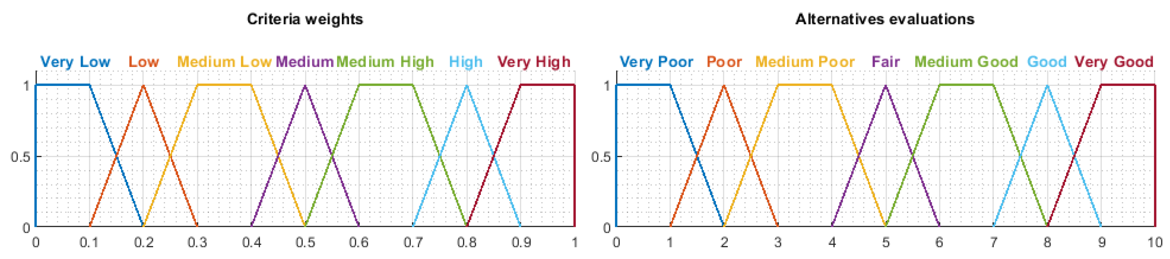
To solve the decision problem, the TFNs-based fuzzy TOPSIS method proposed by Chen et al. [28] and modified by Ziemba et al. was used [27]. This method allows K experts to consider a multi-criteria decision problem composed of m alternatives and n criteria. Criteria weights and assessments of alternatives are expressed in the form of TFNs, where ${\tilde{x}}_{ijk}=\left(a_{ijk},b_{ijk},c_{ijk},d_{ijk}\right)$ represents the assessment of the i-th alternative for the j-th criterion expressed by the k-th stakeholder, and ${\tilde{w}}_{jk}=\left(w_{jk1},w_{jk2},w_{jk3},w_{jk4}\right)$ denotes the weight of the j-th criterion expressed by the k-th expert. Criterion weights and evaluation of alternatives are defined using the 7-point linguistic scales presented in Figure 1.

Weights and expert assessments are aggregated to the TFNs form, respectively ${\tilde{w}}_j=\left(w_{j1},w_{j2},w_{j3},w_{j4}\right)$ and ${\tilde{x}}_{ij}=\left(a_{ij},b_{ij},c_{ij},d_{ij}\right)$, using the modified Similarity Aggregation Method (m-SAM), developed by Ziemba et al. and presented in [27].

According to the m-SAM procedure, for each pair of experts k, l and each j-th weight, the agreement degree $S\left({\tilde{w}}_{jk},{\tilde{w}}_{jl}\right)$ is determined, according to the Formula (1):

$$S\left({\tilde{w}}_{jk},{\tilde{w}}_{jl}\right)=\{\begin{array}{c}\frac{{{\displaystyle \int }}_x^{}(\min \{{\mu }_{{\tilde{w}}_{jk}}\left(x\right),{\mu }_{{\tilde{w}}_{jl}}\left(x\right)\})\mathrm{d}x}{{{\displaystyle \int }}_x^{}(\max \{{\mu }_{{\tilde{w}}_{jk}}\left(x\right),{\mu }_{{\tilde{w}}_{jl}}\left(x\right)\})\mathrm{d}x}for{{\displaystyle \int }}_x^{}(\max \{{\mu }_{{\tilde{w}}_{jk}}\left(x\right),{\mu }_{{\tilde{w}}_{jl}}\left(x\right)\})dx>0,\\ 0for{{\displaystyle \int }}_x^{}(\max \{{\mu }_{{\tilde{w}}_{jk}}\left(x\right),{\mu }_{{\tilde{w}}_{jl}}\left(x\right)\})dx=0,\end{array}$$

(1)

Then an agreement matrix is constructed containing the agreement degrees $S\left({\tilde{w}}_{jk},{\tilde{w}}_{jl}\right)$ according to the Formula (2):

$$AM=\left[\begin{array}{cc}\begin{array}{cc}1& S\left({\tilde{w}}_{j1},{\tilde{w}}_{j2}\right)\\ S\left({\tilde{w}}_{j2},{\tilde{w}}_{j1}\right)& 1\end{array}& \begin{array}{cc}\cdots & S\left({\tilde{w}}_{j1},{\tilde{w}}_{jK}\right)\\ \cdots & S\left({\tilde{w}}_{j2},{\tilde{w}}_{jK}\right)\end{array}\\ \begin{array}{cc}⋮& ⋮\\ S\left({\tilde{w}}_{jK},{\tilde{w}}_{j1}\right)& S\left({\tilde{w}}_{jK},{\tilde{w}}_{j2}\right)\end{array}& \begin{array}{cc}\ddots & ⋮\\ \cdots & 1\end{array}\end{array}\right]$$

(2)

In the next step, the mean agreement degree is calculated for each stakeholder (3):

$$A\left(E_k\right)=\frac{1}{K-1}{{\displaystyle \sum }}_{\begin{array}{c}l=1\\ l\ne k\end{array}}^{K}S\left({\tilde{w}}_{jk},{\tilde{w}}_{jl}\right)$$

(3)

Then the relative agreement degree (RAD) is calculated for each expert (4):

$$RA{D}_k=\{\begin{array}{c}\frac{A\left(E_k\right)}{{{\displaystyle \sum }}_{k=1}^{K}A\left(E_k\right)}for{\displaystyle \sum }_{k=1}^{K}A\left(E_k\right)>0,\\ e_{k}for{\displaystyle \sum }_{k=1}^{K}A\left(E_k\right)=0.\end{array}$$

(4)

where $e_k$ denotes the importance of the k-th expert, where $\sum _{k=1}^K{e}_k=1$.

On the basis of the RAD calculated for each expert, his consensus degree coefficient (CDC) is determined, according to the Formula (5):

$$CD{C}_k=\beta ·e_k+\left(1-\beta \right)·RA{D}_k$$

(5)

where $\beta \in 0,1$ is the coefficient of participation of $RA{D}_k$ and $e_k$ in the CDC. When $\beta =0$ consensus degree coefficient equals relative agreement degree ($CD{C}_k=RA{D}_k)$, and for $\beta =1$, consensus degree coefficient depends solely on expert rank ($CD{C}_k=e_k$).

The aggregation of weights into the form ${\tilde{w}}_j=\left(w_{j1},w_{j2},w_{j3},w_{j4}\right)$ is performed using the Formula (6):

$${\tilde{w}}_j={{\displaystyle \sum }}_{k=1}^K({\tilde{w}}_{jk}⨂CD{C}_k)={{\displaystyle \sum }}_{k=1}^K\left(w_{jk1}\times CD{C}_k,w_{jk2}\times CD{C}_k,w_{jk3}\times CD{C}_k,w_{jk4}\times CD{C}_k\right)$$

(6)

Analogous m-SAM procedure steps are performed to aggregate expert assessments ${\tilde{x}}_{ijk}$.

Based on the aggregated assessments of alternatives, a fuzzy decision matrix (7) and a vector of weights (8) are constructed:

$$\tilde{D}=\left[\begin{array}{cc}\begin{array}{cc}{\tilde{x}}_{11}& {\tilde{x}}_{12}\\ {\tilde{x}}_{21}& {\tilde{x}}_{22}\end{array}& \begin{array}{cc}\cdots & {\tilde{x}}_{1n}\\ \cdots & {\tilde{x}}_{2n}\end{array}\\ \begin{array}{cc}⋮& ⋮\\ {\tilde{x}}_{m1}& {\tilde{x}}_{m2}\end{array}& \begin{array}{cc}\ddots & ⋮\\ \cdots & {\tilde{x}}_{mn}\end{array}\end{array}\right]$$

(7)

$$\tilde{W}=\left[{\tilde{w}}_1,{\tilde{w}}_2,\dots ,{\tilde{w}}_n\right]$$

(8)

Then the evaluations of alternatives ${\tilde{x}}_{ij}=\left(a_{ij},b_{ij},c_{ij},d_{ij}\right)$ are normalized. Formula (9) is used for benefit criteria, and the normalization for cost criteria is according to Formula (10):

$${\tilde{p}}_{ij}=\left(\frac{a_{ij}}{d_j^{*}},\frac{b_{ij}}{d_j^{*}},\frac{c_{ij}}{d_j^{*}},\frac{d_{ij}}{d_j^{*}}\right),\mathrm{where}{d}_j^{*}=\underset{i}{\max }{d}_{ij}$$

(9)

$${\tilde{p}}_{ij}=\left(\frac{a_j^{-}}{d_{ij}},\frac{a_j^{-}}{c_{ij}},\frac{a_j^{-}}{b_{ij}},\frac{a_j^{-}}{a_{ij}}\right),\mathrm{where}{a}_j^{-}=\underset{i}{\min }{a}_{ij}$$

(10)

In the next step, a normalized fuzzy decision matrix is built (11):

$$\tilde{P}=\left[\begin{array}{cc}\begin{array}{cc}{\tilde{p}}_{11}& {\tilde{p}}_{12}\\ {\tilde{p}}_{21}& {\tilde{p}}_{22}\end{array}& \begin{array}{cc}\cdots & {\tilde{p}}_{1n}\\ \cdots & {\tilde{p}}_{2n}\end{array}\\ \begin{array}{cc}⋮& ⋮\\ {\tilde{p}}_{m1}& {\tilde{p}}_{m2}\end{array}& \begin{array}{cc}\ddots & ⋮\\ \cdots & {\tilde{p}}_{mn}\end{array}\end{array}\right]$$

(11)

After taking into account the weights of the criteria, the weighted normalized fuzzy decision matrix is obtained, the elements of which are calculated according to Formula (12):

$${\tilde{v}}_{ij}={\tilde{p}}_{ij}\otimes {\tilde{w}}_j$$

(12)

Based on weighted normalized fuzzy decision matrix, the fuzzy positive-ideal solution (FPIS) (13) and the fuzzy negative-ideal solution (FNIS) are calculated (14):

$$FPI{S}^{*}=\left({\tilde{v}}_1^{*},{\tilde{v}}_2^{*},\dots ,{\tilde{v}}_n^{*}\right),\mathrm{where}{\tilde{v}}_j^{*}=\underset{i}{\max }\left\{{\tilde{v}}_{ij4}\right\}$$

(13)

$$FNI{S}^{-}=\left({\tilde{v}}_1^{-},{\tilde{v}}_2^{-},\dots ,{\tilde{v}}_n^{-}\right),\mathrm{where}{\tilde{v}}_j^{-}=\underset{i}{\min }\left\{{\tilde{v}}_{ij1}\right\}$$

(14)

The distances of the i-th alternative from FPIS ($d_i^{*}$) are calculated according to Formula (15), and the Formula (16) is used to determine FNIS ($d_i^{-}$) (16):

$$d_i^{*}={{\displaystyle \sum }}_{j=1}^n{d}_v\left({\tilde{v}}_{ij},{\tilde{v}}_j^{*}\right)$$

(15)

$$d_i^{-}={{\displaystyle \sum }}_{j=1}^n{d}_v\left({\tilde{v}}_{ij},{\tilde{v}}_j^{-}\right)$$

(16)

where $d_v\left(\tilde{x},\tilde{y}\right)$ is a crisp measure of the distance between two TFNs, determined using the Formula (17):

$$d_v\left(\tilde{x},\tilde{y}\right)=\sqrt{\frac{1}{4}\left[{\left(x_1-y_1\right)}^2+{\left(x_2-y_2\right)}^2+{\left(x_3-y_3\right)}^2+{\left(x_4-y_4\right)}^2\right]}$$

(17)

The overall assessment of the i-th alternative is expressed by the closeness coefficient determining the distance of the obtained solution from FPIS and FNIS according to the Formula (18):

$$C{C}_i=\frac{d_i^{-}}{d_i^{*}+d_i^{-}}$$

(18)

Depending on the obtained value of $C{C}_i$, the considered alternative may belong to one of several classes of assessment status defined in the literature [28,29]:

• if $C{C}_i\in [0,0.2)$ then $A_i$ belongs to Class I–‘not recommended’,
• if $C{C}_i\in [0.2,0.4)$ then $A_i$ belongs to Class II–‘recommended with high risk’,
• if $C{C}_i\in [0.4,0.6)$ then $A_i$ belongs to Class III–‘recommended with low risk’,
• if $C{C}_i\in [0.6,0.8)$ then $A_i$ belongs to Class IV–‘approved’,
• if $C{C}_i\in \left[0.8,1\right]$ then $A_i$ belongs to Class V–‘approved and strictly preferred’.

The fuzzy TOPSIS method may use TFNs, triangular fuzzy numbers (where $b_{ijk}=c_{ijk}$ or $w_{jk2}=w_{jk3}$), interval numbers (where $a_{ijk}=b_{ijk}$ and $c_{ijk}=d_{ijk}$ or $w_{jk1}=w_{jk2}$ and $w_{jk3}=w_{jk4}$), and even crisp numbers represented in the form of singletons (where $a_{ijk}=b_{ijk}=c_{ijk}=d_{ijk}$ or $w_{jk1}=w_{jk2}=w_{jk3}=w_{jk4}$). In the fuzzy TOPSIS method, both numerical and linguistic values can be used.

2.2. Model of the Decision Problem

The assessment of planned investments in offshore wind farms required the construction of a decision model, which includes a set of m alternatives and n criteria, assessed by K experts. Three field experts ($E_1$–$E_3$), who were impartial scientists experienced in RES research, including wind energy, helped to solve the decision problem.

Identification of the alternatives was carried out on the basis of scientific publications and reports [10,11] indicating 6 offshore wind farms to be launched in Poland by 2030. These alternatives are shown in Figure 2 [10,11,30].

The next step was to define the evaluation criteria used in the decision problem. Literature review [14,18,19,20,21,22], analysis of available information on planned investments [31,32,33,34,35,36,37] and consultation with field experts made it possible to indicate the criteria presented in

Table 1. Criteria for assessing offshore wind farms projects.

No.	Group	Criterion	Unit	Preference Direction	Reference
C1	Technical	Average annual wind speed	(m/s)	max	[14,19,20,21,22]
C2	Social	Shipping density	linguistic	max	[14,18,19,20,21]
C3	Social	Fishing density	linguistic	max	[18]
C4	Technical	Geotechnical conditions	linguistic	max	[18,20,21,22]
C5	Spatial	Proximity to hydrocarbon reserves	linguistic	max	[14,22]
C6	Spatial	Proximity to protected areas	linguistic	max	[14,18,19,22]
C7	Spatial	Proximity to shore	(km)	min	[14,18,19,20,22]
C8	Technical	Sea water depth	(m)	min	[14,18,20,21,22]
C9	Environmental	Pollutant reduction effect	(tonnes)	max	[21]
C10	Economic	Expected impact on GDP (economic externalities)	(million PLN)	max	[14]
C11	Social	Employment	(jobs)	max	[14,19,20,21]
C12	Economic	Initial investment cost	(million PLN)	min	[14,18,20,21,22]
C13	Economic	Investment payback period	(years)	min	[14,18,20,21,22]

.

Experts $E_1$–$E_3$ individually determined the weights of the criteria presented in

Table 2. Criteria weights assigned by individual stakeholders.

No.	Criterion	${\mathit{E}}_1$	${\mathit{E}}_2$	${\mathit{E}}_3$
C1	Average annual wind speed	VH	H	H
C2	Shipping density	MH	H	MH
C3	Fishing density	MH	H	MH
C4	Geotechnical conditions	H	MH	M
C5	Proximity to hydrocarbon reserves	M	M	MH
C6	Proximity to protected areas	M	MH	VH
C7	Proximity to shore	H	M	M
C8	Sea water depth	H	ML	M
C9	Pollutant reduction effect	M	MH	VH
C10	Expected impact on GDP (economic externalities)	VH	MH	M
C11	Employment	H	H	MH
C12	Initial investment cost	H	M	MH
C13	Investment payback period	VH	M	MH

VL—very low, L—low, ML—medium low, M—medium, MH—medium high, H—high, VH—very high

.

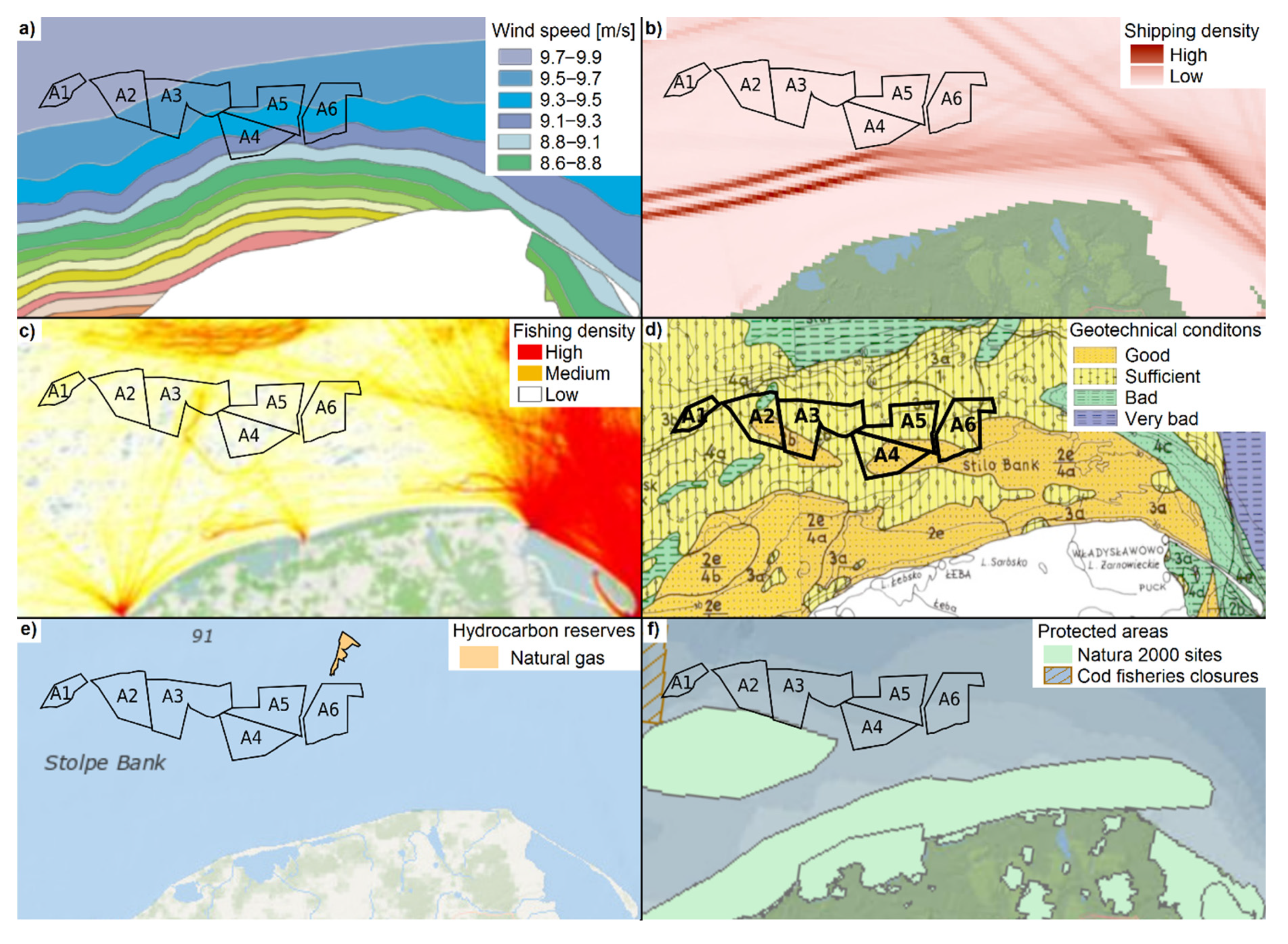
The assessment of alternatives in terms of individual criteria was carried out linguistically and numerically by experts and based on commonly available numerical data. Figure 3 presents information on the locations provided for the considered wind farms in the scope of: (a) wind speed [38], (b) shipping density [39], (c) fishing density [40], (d) geotechnical conditions [41], (e) proximity to hydrocarbon reserves [42], (f) proximity to protected areas [39]. Based on the information presented graphically in Figure 3, the three field experts linguistically assessed the alternatives against the C2–C6 criteria and the assigned numerical TFNs values for C1 criterion.

Then, using publicly available data on individual offshore wind farms projects [31,32,33,34,35,36,37], TFNs were defined for the C7–C8 criteria. In turn, the values of the C10–C12 criteria were calculated as the product of the planned capacity of individual wind farms and the following conversion factors:

• for C10—expected GDP growth per 1 MW—the assumed value was 10 ± 10% PLN million [12], so it was $\widetilde{\mathrm{TFN}}=\left(9,10,10,11\right)$,
• for C11—employment per 1 MW—the number of jobs was 12.8 ± 10% [12], so it was $\widetilde{\mathrm{TFN}}=\left(11.52,12.8,12.8,14.08\right)$,
• for C12—investment cost for 1 MW—the value of 4 ± 10% million Euro was assumed [12], which after conversion into PLN gave 18 ± 10% PLN million, so it was $\widetilde{\mathrm{TFN}}=\left(16.2,18,18,19.8\right)$.

The values of the C7–C8 and C10–C12 criteria were the same for all experts and independent of them.

Calculating the values of the C9 and C13 criteria, it was necessary to determine the amount of annual energy production $\tilde{E}$ (MWh). It was in the form of TFN estimated as the product of the wind turbine output power, the number of turbines and the number of 8760 h [43]. The turbine output power $\widetilde{P_W}$ (MW) was the TFN calculated from the Formula (19) [44]:

$$\widetilde{P_W}=\frac{\rho \ast A_r\ast C_p}{\mathrm{2,000,000}}⨂{\tilde{v}}^3$$

(19)

where $\rho$ is air density (kg/m³), $A_r$ this is the turbine rotor blades swept area (m²), $C_p$ is the power coefficient of the wind turbine, and $\tilde{v}$ is wind speed (m/s). The values $\rho$, $A_r$, $C_p$ were crisp numbers, and $\tilde{v}$ was TFN, taken directly from C1 criterion. Based on [45], air density $\rho =1.23$ kg/m³ was assumed. When determining the turbine rotor blades swept area, it was assumed that during the construction period of individual power plants, wind turbines more advanced than now would be available, and therefore the value $A_r=\mathrm{39,000}$ m² was adopted, taken from the specification of the SG 14-222 DD turbine [46] which can be used in Polish offshore projects [47]. Moreover, based on the theoretical maximum power coefficient value of 0.593 (Betz limit), a practical power coefficient value in the range of 0.4–0.5 [48] was adopted $C_p=0.48$. As for the number of turbines, this number was calculated as the quotient of the planned capacity of a given wind farm and the maximum output power of the SG 14-222 DD (14 MW) turbine [46], rounding the result down to integers.

Having determined the fuzzy value of the annual produced energy $\tilde{E}$, the value of the C9 criterion was calculated as the product of $\tilde{E}$ and the CO₂ emission factor for electricity in Poland. This coefficient for 2018 was 0.792 tonnes/MWh [49], and the study assumed its values as 0.792 ± 10% tonnes/MWh, so it was represented by $\widetilde{\mathrm{TFN}}=\left(0.7128,0.792,0.792,0.8712\right)$.

In determining the value of the C13 criterion, it was necessary to estimate the annual revenues, operation and maintenance costs and on that basis calculate the annual profits. The income ($\widetilde{Income}$) was calculated as the product of the annual energy production $\tilde{E}$ and the reference price of 1 MWh of energy obtained from an offshore wind farm. This price in 2020 in Poland was 450 PLN/MWh [50], and the research assumed the value of 450 ± 10% PLN/MWh, so it was represented by $\widetilde{\mathrm{TFN}}=\left(405,450,450,495\right)$. Operation and maintenance costs ($\widetilde{OM}$) were calculated as the product of the annual energy production $\tilde{E}$ and the annual operation and maintenance costs per 1 MWh, estimated at approximately 30 Euro [51], which after conversion into PLN and taking into account 10% deviation gives the value of 135 ± 10% PLN, so $\widetilde{\mathrm{TFN}}=\left(121.5,135,135,148.5\right)$. Therefore, the annual profits expressed in PLN million were calculated using the rules of fuzzy arithmetic [28] according to the Formula (20):

$$\widetilde{Profit}=\frac{\widetilde{Income}-\widetilde{OM}}{\mathrm{1,000,000}}=\frac{\left(Incom{e}_1-O{M}_4,Incom{e}_2-O{M}_3,Incom{e}_3-O{M}_2,Incom{e}_4-O{M}_1\right)}{\mathrm{1,000,000}}$$

(20)

Finally, the C13 criterion, i.e., the payback period was calculated as the quotient of the C12 criterion, i.e., the investment cost $\widetilde{I\_cost}$ and the annual profit ($\widetilde{Profit}$) according to the rules of fuzzy arithmetic (21):

$$\widetilde{Pp}=\widetilde{I\_cost}\oslash \widetilde{Profit}=\left(\frac{I\_cos{t}_1}{Profi{t}_4},\frac{I\_cos{t}_2}{Profi{t}_3},\frac{I\_cos{t}_3}{Profi{t}_2},\frac{I\_cos{t}_4}{Profi{t}_1}\right)$$

(21)

Table 3. Assessments of expert alternatives $E_1$.

	C1	C2	C3	C4	C5	C6	C9	C13
A1	(9.7, 9.7, 9.9, 9.9)	VG	F	MG	VG	F	(1,640,242, 1,822,491, 1,937,563, 2,131,319)	(6.08, 7.97, 8.93, 12.18)
A2	(9.5, 9.7, 9.7, 9.9)	VG	G	MG	VG	MP	(5,238,929, 6,196,470, 6,196,470, 7,246,486)	(6.02, 8.76, 8.76, 13.64)
A3	(9.3, 9.5, 9.7, 9.9)	VG	MP	G	VG	MP	(6,187,075, 7,327,652, 7,800,263, 9,122,047)	(5.87, 8.47, 9.51, 15.12)
A4	(8.8, 9.1, 9.3, 9.5)	F	G	VG	VG	MG	(2,057,548, 2,528,039, 2,698,413, 3,163,902)	(6.71, 9.79, 11.06, 18.86)
A5	(9.1, 9.3, 9.5, 9.7)	G	MG	G	G	G	(4,008,747, 4,754,346, 5,067,722, 5,934,032)	(6.30, 9.09, 10.24, 16.34)
A6	(9.1, 9.3, 9.5, 9.7)	F	F	G	MG	VG	(4,604,642, 5,461,073, 5,821,032, 6,816,117)	(6.29, 9.08, 10.23, 16.33)

VP—very poor, P—poor, MP—medium poor, F—fair, MG—medium good, G—good, VG—very good.

,

Table 4. Assessments of expert alternatives $E_2$.

	C1	C2	C3	C4	C5	C6	C9	C13
A1	(9.7, 9.7, 9.9, 9.9)	G	F	MG	VG	MP	(1,640,242, 1,822,491, 1,937,563, 2,131,319)	(6.08, 7.97, 8.93, 12.18)
A2	(9.5, 9.7, 9.9, 9.9)	G	G	F	VG	P	(5,238,929, 6,196,470, 6,587,714, 7,246,486)	(6.02, 8.03, 9.00, 13.64)
A3	(9.5, 9.7, 9.7, 9.9)	MG	P	G	VG	P	(6,594,887, 7,800,263, 7,800,263, 9,122,047)	(5.97, 8.69, 8.69, 13.52)
A4	(8.9, 9.1, 9.4, 9.5)	MP	F	G	VG	F	(2,128,492, 2,528,039, 2,786,398, 3,163,902)	(6.77, 9.37, 11.23, 17.72)
A5	(9.1, 9.3, 9.5, 9.6)	F	F	MG	MG	G	(4,008,747, 4,754,346, 5,067,722, 5,752,390)	(6.55, 9.09, 10.24, 15.95)
A6	(9.1, 9.3, 9.5, 9.6)	P	P	MG	F	VG	(4,604,642, 5,461,073, 5,821,032, 6,607,475)	(6.54, 9.08, 10.23, 15.94)

and

Table 5. Assessments of expert alternatives $E_3$.

	C1	C2	C3	C4	C5	C6	C9	C13
A1	(9.7, 9.7, 9.9, 9.9)	G	MG	MG	VG	MP	(1,640,242, 1,822,491, 1,937,563, 2,131,319)	(6.08, 7.97, 8.93, 12.18)
A2	(9.5, 9.7, 9.7, 9.9)	VG	G	F	VG	P	(5,238,929, 6,196,470, 6,196,470, 7,246,486)	(6.02, 8.76, 8.76, 13.64)
A3	(9.4, 9.6, 9.7, 9.9)	G	MP	G	VG	P	(6,388,812, 7,561,496, 7,800,263, 9,122,047)	(5.92, 8.57, 9.08, 14.29)
A4	(8.8, 9.1, 9.3, 9.5)	MP	MG	G	VG	F	(2,057,548, 2,528,039, 2,698,413, 3,163,902)	(6.71, 9.79, 11.06, 18.86)
A5	(9.2, 9.3, 9.5, 9.6)	MG	F	G	MG	G	(4,142,361, 4,754,346, 5,067,722, 5,752,390)	(6.61, 9.09, 10.24, 15.07)
A6	(9.1, 9.3, 9.5, 9.7)	MP	MP	G	F	VG	(4,604,642, 5,461,073, 5,821,032, 6,816,117)	(6.29, 9.08, 10.23, 16.33)

show the ratings assigned to alternatives by individual experts. Since the values of the C7–C8 and C10–C12 criteria were the same for all experts, they are presented separately in

Table 6. Assessments of alternatives common for experts $E_1$–$E_3$.

	C7	C8	C10	C11	C12
A1	(55, 55, 55, 55)	(45, 45, 45, 45)	(3150, 3500, 3500, 3850)	(4032, 4480, 4480, 4928)	(5670, 6300, 6300, 6930)
A2	(37, 37, 37, 40)	(23, 30, 30, 41)	(10,800, 12,000, 12,000, 13,200)	(13,824, 15,360, 15,360, 16,896)	(19,440, 21,600, 21,600, 23,760)
A3	(25, 30, 30, 40)	(20, 40, 40, 60)	(13,482, 14,980, 14,980, 16,478)	(17,257, 19,174, 19,174, 21,092)	(24,267.6, 26,964, 26,964, 29,660.4)
A4	(22, 22, 23, 30)	(25, 30, 30, 39)	(5400, 6,000, 6000, 6,600)	(6912, 7680, 7680, 8448)	(9720, 10800, 10,800, 11,880)
A5	(25, 33, 33, 34)	(20, 40, 40, 60)	(9409.5, 10,455, 10,455, 11,500.5)	(12,044, 13,382, 13,382, 14,721)	(16,937.1, 18,819, 18,819, 20,700.9)
A6	(23, 23, 28, 28)	(40, 40, 40, 40)	(10,800, 12,000, 12,000, 13,200)	(13,824, 15,360, 15,360, 16,896)	(19,440, 21,600, 21,600, 23,760)

. Table 2, Table 3, Table 4, Table 5 and Table 6 therefore illustrate a model of the decision problem solved subsequently with the modified fuzzy TOPSIS method.

3. Results

The study assumes that the rank of experts is equal ($e_1=e_2=e_3$). Therefore, each of the experts had the same effect on the form of the fuzzy decision matrix aggregated using the m-SAM procedure. Moreover, the value of the coefficients $\beta =0.5$ was assumed, so the consensus among experts was of the same importance as the ranks of experts. As a result of the aggregation of individual weights of the criteria (see: Table 2), the aggregated weights presented in

Table 7. Aggregated expert criteria weights.

No.	Criterion	Weight Aggregated
C1	Average annual wind speed	(0.7212, 0.8212, 0.8424, 0.9212)
C2	Shipping density	(0.541, 0.641, 0.7205, 0.8205)
C3	Fishing density	(0.541, 0.641, 0.7205, 0.8205)
C4	Geotechnical conditions	(0.5292, 0.6292, 0.6708, 0.7708)
C5	Proximity to hydrocarbon reserves	(0.4205, 0.5205, 0.541, 0.641)
C6	Proximity to protected areas	(0.5083, 0.6083, 0.6667, 0.75)
C7	Proximity to shore	(0.45, 0.55, 0.55, 0.65)
C8	Sea water depth	(0.3667, 0.4667, 0.5083, 0.6083)
C9	Pollutant reduction effect	(0.5083, 0.6083, 0.6667, 0.75)
C10	Expected impact on GDP (economic externalities)	(0.5083, 0.6083, 0.6667, 0.75)
C11	Employment	(0.659, 0.759, 0.7795, 0.8795)
C12	Initial investment cost	(0.5292, 0.6292, 0.6708, 0.7708)
C13	Investment payback period	(0.5083, 0.6083, 0.6667, 0.75)

were obtained.

Furthermore, the aggregation of experts’ assessments in the group assessment allowed the fuzzy decision matrix presented in

Table 8. Aggregated assessments of alternatives—transposed fuzzy decision matrix.

	A1	A2	A3	A4	A5	A6
C1	(9.7, 9.7, 9.9, 9.9)	(9.5, 9.7, 9.7619, 9.9)	(9.3989, 9.5989, 9.7, 9.9)	(8.832, 9.1, 9.332, 9.5)	(9.1328, 9.3, 9.5, 9.633)	(9.1, 9.3, 9.5, 9.6674)
C2	(7.2121, 8.2121, 8.4242, 9.2121)	(7.7878, 8.7878, 9.5757, 9.7878)	(6.7458, 7.7458, 8.3291, 9.0250)	(2.4102, 3.4102, 4.2051, 5.2051)	(5.2916, 6.2916, 6.7083, 7.7083)	(2.2916, 3.2916, 3.7083, 4.7083)
C3	(4.2051, 5.2051, 5.4102, 6.4102)	(7, 8, 8, 9)	(1.7948, 2.7948, 3.5897, 4.5897)	(5.2916, 6.2916, 6.7083, 7.7083)	(4.2051, 5.2051, 5.4102, 6.4102)	(2.2916, 3.2916, 3.7083, 4.7083)
C4	(5, 6, 7, 8)	(4.2051, 5.2051, 5.4102, 6.4102)	(7, 8, 8, 9)	(7.2121, 8.2121, 8.4242, 9.2121)	(6.5897, 7.5897, 7.7948, 8.7948)	(6.5897, 7.5897, 7.7948, 8.7948)
C5	(8, 9, 10, 10)	(8, 9, 10, 10)	(8, 9, 10, 10)	(8, 9, 10, 10)	(5.4102, 6.4102, 7.2051, 8.2051)	(4.2051, 5.2051, 5.4102, 6.4102)
C6	(2.4102, 3.4102, 4.2051, 5.2051)	(1.2051, 2.2051, 2.4102, 3.4102)	(1.2051, 2.2051, 2.4102, 3.4102)	(4.2051, 5.2051, 5.4102, 6.4102)	(7, 8, 8, 9)	(8, 9, 10, 10)
C7	(55, 55, 55, 55)	(37, 37, 37, 40)	(25, 30, 30, 40)	(22, 22, 23, 30)	(25, 33, 33, 34)	(23, 23, 28, 28)
C8	(45, 45, 45, 45)	(23, 30, 30, 41)	(20, 40, 40, 60)	(25, 30, 30, 39)	(20, 40, 40, 60)	(40, 40, 40, 40)
C9	(1,640,242.1533, 1,822,491.2815, 1,937,563.0351, 2,131,319.3386)	(5,238,928.8334, 6,196,470.3571, 6,322,907.4134, 7,246,485.7514)	(6,389,788.3162, 7,562,593.1408, 7,800,262.6849, 9,122,046.7694)	(2,080,698.7304, 2,528,038.6844, 2,727,123.918, 3,163,902.119)	(4,053,106.5539, 4,754,346.315, 5,067,722.0088, 5,812,423.8934)	(4,604,641.8894, 5,461,073.4699, 5,821,032.0371, 6,747,564.3523)
C10	(3150, 3500, 3500, 3850)	(10,800, 12,000, 12,000, 13,200)	(13,482, 14,980, 14,980, 16,478)	(5400, 6000, 6000, 6600)	(9409.5, 10455, 10,455, 11,500.5)	(10,800, 12,000, 12,000, 13,200)
C11	(4032, 4480, 4480, 4928)	(13,824, 15,360, 15,360, 16,896)	(17,257, 19,174, 19,174, 21,092)	(6912, 7680, 7680, 8448)	(12,044, 13,382, 13,382, 14,721)	(13,824, 15,360, 15,360, 16,896)
C12	(5670, 6300, 6300, 6930)	(19,440, 21,600, 21,600, 23,760)	(24,267.6, 26,964, 26,964, 29,660.4)	(9720, 10,800, 10,800, 11,880)	(16,937.1, 18,819, 18,819, 20,700.9)	(19,440, 21,600, 21,600, 23,760)
C13	(6.0876, 7.9723, 8.9331, 12.1864)	(6.0291, 8.5276, 8.844, 13.6436)	(5.9282, 8.5804, 9.0987, 14.3181)	(6.736, 9.6587, 11.1171, 18.4928)	(6.4873, 9.0957, 10.2415, 15.7972)	(6.3784, 9.0888, 10.2337, 16.2075)

to be obtained. To increase readability, the fuzzy decision matrix in Table 8 has been transposed.

Table 8 is supplemented by Figure 4 presenting aggregated fuzzy assessments of alternatives in a graphical form.

The next steps were normalization and then weighting of the fuzzy decision matrix. On the basis of the weighted normalized fuzzy decision matrix, the FPIS and FNIS were determined, which were used to determine the overall assessment and ranking of alternatives, presented in

Table 9. Ranking of offshore wind farms planned in Poland in the coming years.

Alternative	A1	A2	A3	A4	A5	A6
$C{C}_i$	0.3645	0.4726	0.4877	0.4034	0.4534	0.4323
Rank	6	2	1	5	3	4
Class of assessment status	II	III	III	III	III	III

.

The obtained ranking shows that the most preferred wind farm is A3, i.e., Baltica 2 with a planned capacity of 1498 MW. It is followed by alternatives A2 (Baltic II–1200 MW), A5 (Baltica 3–1045.5 MW), A6 (Baltic Power–1200 MW) and A4 (Baltic 3–600 MW). All these alternatives belong to the “recommended with low risk” class of assessment status, however A4 is at the lower end of this class. The last place in the ranking is taken by A1 (FEW Baltic II–350 MW) belonging to the lower class of assessment status, i.e., “recommended with high risk”. It may seem that the developed decision model favors the wind farm with the higher capacity, but it should be stated that capacity is not the only factor determining the order of alternatives. The analysis of Table 8 and Figure 4 shows that the C10 and C11 criteria of the benefit type, directly dependent on the capacity, prefer alternatives with a higher capacity, but the C12 cost criterion partially reduces this effect. Based on Figure 4, it can also be noticed that the most preferred A3 alternative, compared to other alternatives, dominates most of the criteria, and is characterized by low efficiency only in terms of the C3, C6, C12. The second-ranked alternative A2 is characterized by high efficiency on the criteria C1–C3, C5, C8–C11, C13, and worse results on the criteria C4, C6, C7, C12. The A5 and A6 alternatives stand out positively primarily in terms of the C6 criterion, they are characterized by average efficiency on most of the criteria, and they lose the most on the C2 and C5 criteria. The alternatives A4 and A1 suffer the greatest losses in terms of capacity, i.e., C10 and C11, as well as C9. Moreover, the A4 alternative has poor efficiency on the C1 and C2 criteria, and A1 loses the most on the C7 and C8 criteria. The ranking presented in Table 9 reflects all these advantages and weaknesses of individual alternatives.

4. Discussion

In the modified fuzzy TOPSIS method, several variables are used that may influence the obtained results. These are in particular: the $\beta$ coefficient, the rank of experts $e_k$ and the weights of the criteria ${\tilde{w}}_{jk}$. Therefore, an analysis of the sensitivity of the solution to changes in the values of these variables was performed, leaving other parameters of the decision model unchanged. Figure 5 shows the sensitivity analysis for the $\beta$ coefficient. The results of this analysis indicate that the obtained ranking is robust to changes in the value of this coefficient.

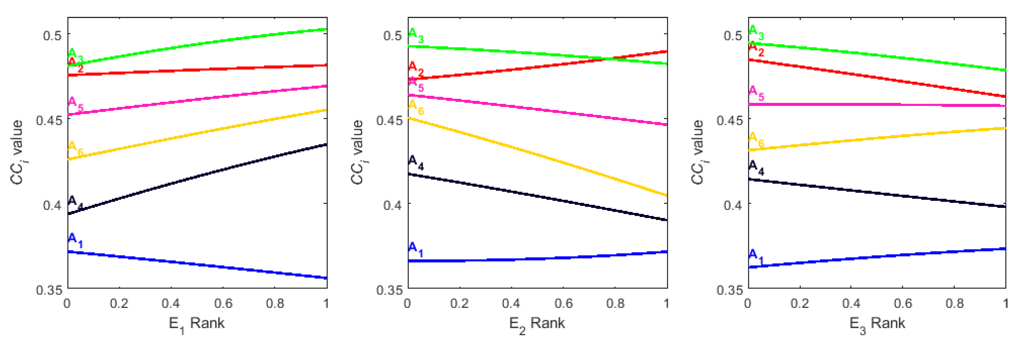
In the sensitivity analysis for the ranks of experts, it was assumed that the rank of the selected expert $e_k$ changes within the range [0,1], while the ranks of the other two experts are equal ($e_p=e_r)$ and proportional to the rank of the selected expert, where $e_k+e_p+e_r=1$. As in Section 3, the value of the $\beta$ coefficient was 0.5. The sensitivity analysis for the ranks of experts is presented in Figure 6. The results show that changes in the ranks of experts, leaving the remaining parameters of the decision model unchanged, do not affect the order of alternatives.

A sensitivity analysis was also performed for expert ranks when the $\beta$ coefficient was 0 and 1, respectively. These analyses are shown in Figure 7 and Figure 8. Figure 7 shows that for $\beta =0$, according to the information provided in Section 2.1, the expert ranks have no significance and in no way affect the obtained ranking of alternatives. On the other hand, Figure 8 shows that for $\beta =1$, i.e., when the agreement between experts is irrelevant, and only the ranks of experts are important, there is a change in the top two places in the ranking with the expert rank $E_2>0.77$. This allows us to draw a more general conclusion that with a sufficiently high value of the $\beta$ coefficient and a high rank of the selected expert, changes in the ranking obtained using the modified fuzzy TOPSIS method may occur. On the other hand, taking into account agreements between experts and seeking consensus has a positive effect on the stability of the obtained rankings of alternatives. Nevertheless, the obtained ranking of offshore wind farms planned in Poland is largely robust to changes in the rank of experts.

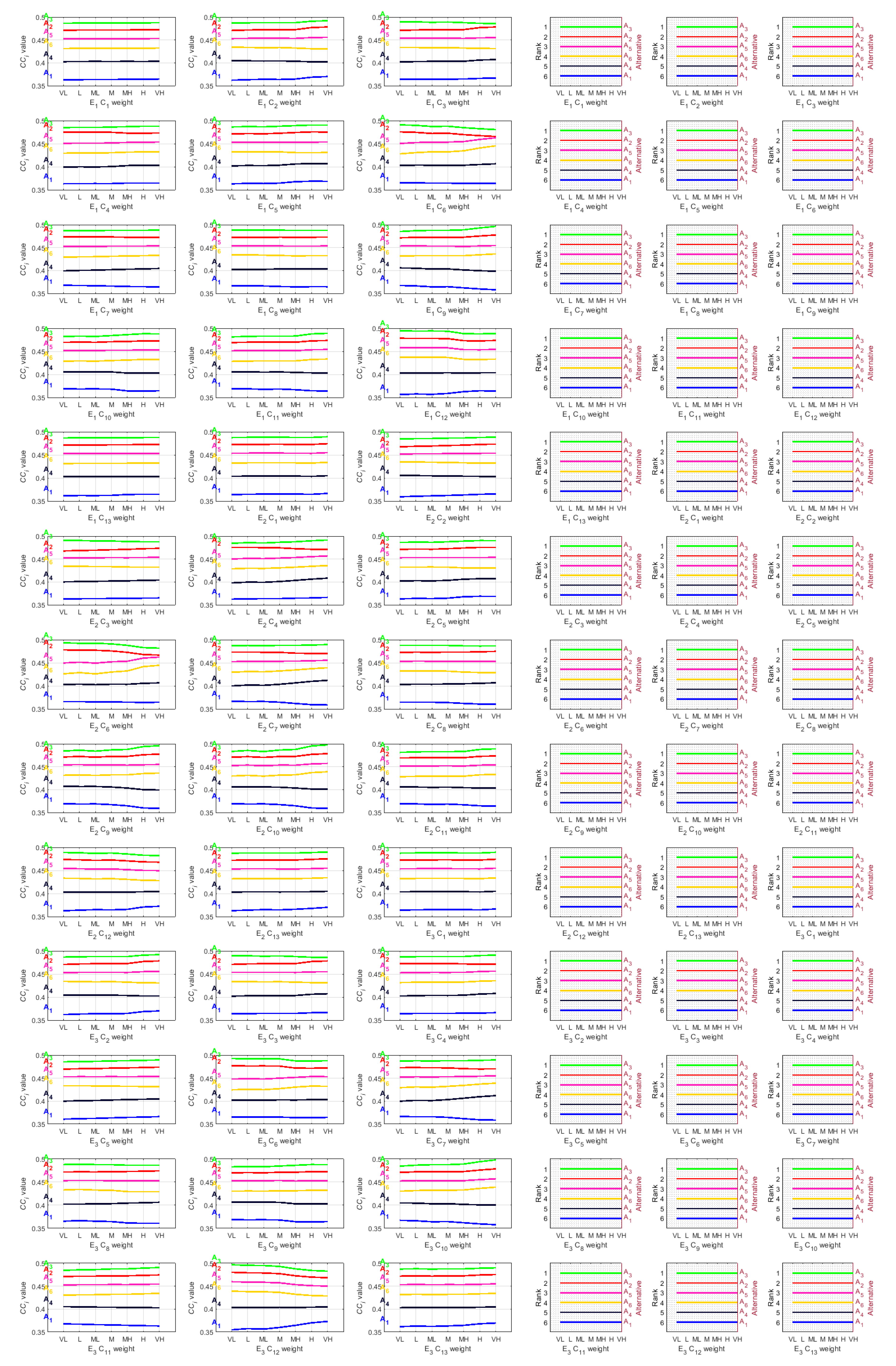
The last sensitivity analysis carried out referred to the criteria weights. These weights were changed separately for each expert, in terms of the linguistic scores {VL−VH}, leaving all other weights unchanged. The results of the analysis are shown in Figure 9. Analyzing Figure 9, it can be concluded that changes in the weight of individual criteria do not cause any changes in the ranking. A more in-depth analysis of Figure 9 shows that as the weights of some criteria are increased, the values of $C{C}_i$ of some alternatives are getting closer, and as a result, with appropriately high weights for this criterion, a change in the position of these alternatives in the ranking can be expected. Specifically, it concerns the weights assigned to the criterion C3 by experts $E_1$ and $E_3$, where increasing these weights causes the results of alternatives A3 and A2 to come closer together, as well as the weights assigned to the criterion C6 by experts $E_1$ and $E_2$, whereby increasing these weights brings the A2 and A5 alternatives closer. This observation established that if the weight of criterion C3 was increased to the value of VH by all experts (without changing the weights of the other criteria), the A3 and A2 alternatives would be equal in the ranking. On the other hand, increasing the weight of the C6 criterion to the VH value by experts $E_1$ and $E_2$ (without changing the weights of other criteria) caused a change in the ranking positions between the A2 and A5 alternatives.

Generalizing the results of the sensitivity analysis, it is necessary to emphasize once again the robustness of the obtained ranking to changes in the value of the $\beta$ coefficient, the ranks of experts $e_k$ and the weighting of the criterion ${\tilde{w}}_{jk}$. Linear changes of one of these factors do not change the ranking, and only a combination of several changes simultaneously may introduce minor changes to the resulting solution. This means that the solution of the decision problem can be considered stable and credible. As for the evaluation of decision alternatives on the basis of sensitivity analysis, the linguistic classes of assessment statuses proposed for the fuzzy TOPSIS method are helpful. On this basis, it can be concluded that the alternatives A3, A2, A5, A6 are stable and in each case considered in the sensitivity analysis, they belong to Class III—”recommended with low risk” ($0.4\le C{C}_i<0.6$). Alternative A1 is equally stable, and in each analyzed situation belongs to Class II—”recommended with high risk” ($C{C}_1<0.4$). On the other hand, the A4 alternative belonging to Class III in practice lies on the border of Class II and Class III ($C{C}_4=0.4034$) and based on the sensitivity analysis, it should be noted that there are possible situations when it will belong to Class II, i.e., assessed as more risky.

5. Conclusions

The aim of the research and its practical contribution was the evaluation of investments in offshore wind farms planned in the coming years in Poland and the indication of the most sustainable investments, characterized by high efficiency and potentially having a strong impact on increasing the dynamics of economic development in the coming years. For reasons of sustainability, potential investments were considered from the perspective of economic, social, environmental, as well as technical and spatial criteria. The study was conducted with the participation of three field experts, which resulted from the need to objectify the assessment and increase the credibility of the obtained results. In addition, in order to study the credibility of the results, a wide sensitivity analysis of the obtained solution was performed. This made it possible to make sure that the obtained ranking of offshore wind farms projects is stable and does not depend on a single factor, the change of which could significantly change the obtained solution. As a result of the research, answers to the research questions posed in the Introduction section were obtained. In Section 2.2, based on a review of the literature, the criteria for assessing offshore wind farms and their values are defined for each investment under consideration. The solution to the decision problem showed that the A3 alternative, i.e., Baltica 2, is the most preferred investment in offshore wind farms planned for the next 10 years in Poland. Based on the linguistic assessment status classes, it can be concluded that all considered alternatives are recommended, however, the alternatives A3, A2, A5, A6, A4 are characterized by a lower risk, while the investment of A1 is assessed as carrying higher risk. Moreover, based on the sensitivity analysis, it can be concluded that there are possible situations where the A4 alternative will be assessed as more risky.

As for the methodological contribution of the article, it is the use of the modified fuzzy TOPSIS method in a decision problem characterized by uncertainty and the development of the application of this method with a broad sensitivity analysis of the obtained solution. In conditions of uncertainty, an appropriate analysis of the sensitivity and robustness of the solution is very important because it allows a rational decision to be made, reducing the knowledge gap of the decision maker [52]. In addition, the analysis of sensitivity and robustness allows for the identification of questionable or accidental solutions recommended only as a result of a specific selection of the values of the decision model parameters. It should be noted that the fuzzy TOPSIS method used in this study also has its limitations. The first limitation is that it is an MCDA method based on a single synthesizing criterion. This means that the fuzzy TOPSIS method, unlike the methods based on the outranking relation, does not allow for the fuzzyfying of preferences [53]. In other words, the fuzzy TOPSIS method does not allow for modelling a situation where it is uncertain whether one of the alternatives is better than the other. The second limitation of the fuzzy TOPSIS method is that during the calculation it is necessary to perform the defuzzification of the evaluation for alternatives and the final calculations are based on crisp numbers (see Formulae (17) and (18)). As a consequence, the decision-maker loses information about the uncertainty of the obtained solution and is unable to assess the potential risk associated with the selection of a specific decision alternative.

Further research directions will include further possible applications of the modified fuzzy TOPSIS method. Among such applications are multi-criteria group decision problems where consensus among decision makers is important, such as website evaluations [54], economic problems [55], urban development [56] or software projects [57]. On the other hand, an interesting research topic is also the assessment of renewable energy sources using other methods that take into account the uncertainty of data and preferences, such as NEAT F-PROMETHEE [58] or stochastic PROSA [59,60].

References

- Altıntaş, H.; Kassouri, Y. The Impact of Energy Technology Innovations on Cleaner Energy Supply and Carbon Footprints in Europe: A Linear versus Nonlinear Approach. J. Clean. Prod. 2020, 276, 124140. [Google Scholar] [CrossRef]
- Paska, J.; Surma, T.; Terlikowski, P.; Zagrajek, K. Electricity Generation from Renewable Energy Sources in Poland as a Part of Commitment to the Polish and EU Energy Policy. Energies 2020, 13, 4261. [Google Scholar] [CrossRef]
- European Commission. 2030 Climate & Energy Framework. Available online: https://ec.europa.eu/clima/policies/strategies/2030_en (accessed on 23 November 2020).
- Paska, J.; Surma, T. Electricity Generation from Renewable Energy Sources in Poland. Renew. Energy 2014, 71, 286–294. [Google Scholar] [CrossRef]
- Brodny, J.; Tutak, M.; Saki, S.A. Forecasting the Structure of Energy Production from Renewable Energy Sources and Biofuels in Poland. Energies 2020, 13, 2539. [Google Scholar] [CrossRef]
- Nemling, O. The Amendment to the Polish Act on Renewable Energy Sources (RES). Available online: https://www.taylorwessing.com/en/insights-and-events/insights/2019/09/the-amendment-to-the-polish-act-on-renewable-energy-sources (accessed on 23 November 2020).
- PWEA—Polish Wind Energy Association. Wind of Hope for Poland’s Green Deal. Available online: http://psew.pl/en/2020/08/25/wind-of-hope-for-polands-green-deal/ (accessed on 11 December 2020).
- Ziemba, P.; Wątróbski, J.; Zioło, M.; Karczmarczyk, A. Using the PROSA Method in Offshore Wind Farm Location Problems. Energies 2017, 10, 1755. [Google Scholar] [CrossRef] [Green Version]
- The Birth of Offshore Wind in Poland. Available online: https://windeurope.org/newsroom/press-releases/the-birth-of-offshore-wind-in-poland/ (accessed on 11 December 2020).
- Gul, A. Innovative Solutions Applied in the High Power Offshore Wind Farms Complex, Taking Intoaccount the Requirements for Protection of the Offshore HVDC Cable Network; Association of Polish Electrical Engineers: Warszawa, Poland, 2 April 2019. [Google Scholar]
- Baltic InteGrid. Recommendations to the ENTSO-E’s Ten Year Network Development Plan; Baltic InteGrid, 2018. [Google Scholar]
- McKinsey & Company. Developing Offshore Wind Power in Poland; McKinsey & Co., 2016. [Google Scholar]
- PWEA—Polish Wind Energy Association. The Future of Offshore Wind in Poland; Polish Wind Energy Association, 2019. [Google Scholar]
- Deveci, M.; Özcan, E.; John, R.; Covrig, C.-F.; Pamucar, D. A Study on Offshore Wind Farm Siting Criteria Using a Novel Interval-Valued Fuzzy-Rough Based Delphi Method. J. Environ. Manag. 2020, 270, 110916. [Google Scholar] [CrossRef]
- Dedecca, J.G.; Hakvoort, R.A.; Ortt, J.R. Market Strategies for Offshore Wind in Europe: A Development and Diffusion Perspective. Renew. Sustain. Energy Rev. 2016, 66, 286–296. [Google Scholar] [CrossRef] [Green Version]
- Nermend, K. The Implementation of cognitive neuroscience techniques for fatigue evaluation in participants of the decision-making process. In Neuroeconomic and Behavioral Aspects of Decision Making; Nermend, K., Łatuszyńska, M., Eds.; Springer International Publishing: Cham, Switzerland, 2017; pp. 329–339. [Google Scholar]
- Nermend, K.; Piwowarski, M.; Borawski, M. Decision Making Methods in Comparative Studies of Complex Economic Processes Management. Iraqi J. Sci. 2020, 652–664. [Google Scholar] [CrossRef] [Green Version]
- Sałabun, W.; Wątróbski, J.; Piegat, A. Identification of a multi-criteria model of location assessment for renewable energy sources. In Artificial Intelligence and Soft Computing; Rutkowski, L., Korytkowski, M., Scherer, R., Tadeusiewicz, R., Zadeh, L.A., Zurada, J.M., Eds.; Springer International Publishing: Cham, Switzerland, 2016; pp. 321–332. [Google Scholar]
- Fetanat, A.; Khorasaninejad, E. A Novel Hybrid MCDM Approach for Offshore Wind Farm Site Selection: A Case Study of Iran. Ocean. Coast. Manag. 2015, 109, 17–28. [Google Scholar] [CrossRef]
- Wu, Y.; Zhang, J.; Yuan, J.; Geng, S.; Zhang, H. Study of Decision Framework of Offshore Wind Power Station Site Selection Based on ELECTRE-III under Intuitionistic Fuzzy Environment: A Case of China. Energy Convers. Manag. 2016, 113, 66–81. [Google Scholar] [CrossRef]
- Gao, J.; Guo, F.; Ma, Z.; Huang, X.; Li, X. Multi-Criteria Group Decision-Making Framework for Offshore Wind Farm Site Selection Based on the Intuitionistic Linguistic Aggregation Operators. Energy 2020, 204, 117899. [Google Scholar] [CrossRef]
- Deveci, M.; Cali, U.; Kucuksari, S.; Erdogan, N. Interval Type-2 Fuzzy Sets Based Multi-Criteria Decision-Making Model for Offshore Wind Farm Development in Ireland. Energy 2020, 198, 117317. [Google Scholar] [CrossRef]
- Ziemba, P. Neat F-Promethee—A New Fuzzy Multiple Criteria Decision Making Method Based on the Adjustment of Mapping Trapezoidal Fuzzy Numbers. Expert Syst. Appl. 2018, 110, 363–380. [Google Scholar] [CrossRef]
- Hwang, C.-L.; Yoon, K. Multiple Attribute Decision Making: Methods and Applications A State-of-the-Art Survey. In Lecture Notes in Economics and Mathematical Systems; Springer: Berlin/Heidelberg, Germany, 1981; ISBN 978-3-540-10558-9. [Google Scholar]
- Piwowarski, M.; Miłaszewicz, D.; Łatuszyńska, M.; Borawski, M.; Nermend, K. Application of the Vector Measure Construction Method and Technique for Order Preference by Similarity Ideal Solution for the Analysis of the Dynamics of Changes in the Poverty Levels in the European Union Countries. Sustainability 2018, 10, 2858. [Google Scholar] [CrossRef] [Green Version]
- Ziemba, P.; Jankowski, J.; Wątróbski, J. Online Comparison System with Certain and Uncertain Criteria Based on Multi-Criteria Decision Analysis Method. In Computational Collective Intelligence; Nguyen, N.T., Papadopoulos, G.A., Jędrzejowicz, P., Trawiński, B., Vossen, G., Eds.; Springer International Publishing: Cham, Switzerland, 2017; pp. 579–589. [Google Scholar]
- Ziemba, P.; Becker, A.; Becker, J. A Consensus Measure of Expert Judgment in the Fuzzy TOPSIS Method. Symmetry 2020, 12, 204. [Google Scholar] [CrossRef] [Green Version]
- Chen, C.-T.; Lin, C.-T.; Huang, S.-F. A Fuzzy Approach for Supplier Evaluation and Selection in Supply Chain Management. Int. J. Prod. Econ. 2006, 102, 289–301. [Google Scholar] [CrossRef]
- Nieto-Morote, A.; Ruz-Vila, F. A Fuzzy Multi-Criteria Decision-Making Model for Construction Contractor Prequalification. Autom. Constr. 2012, 25, 8–19. [Google Scholar] [CrossRef] [Green Version]
- Global Offshore Renewable Map | 4C Offshore. Available online: https://www.4coffshore.com/offshorewind/ (accessed on 11 December 2020).
- The Renewables Consulting Group (RCG). Global Renewable Infrastructure Project (GRIP) Database. Available online: https://grip.thinkrcg.com/ (accessed on 23 November 2020).
- Wind Farms—Online Access—The Wind Power—Wind Energy Market Intelligence. Available online: https://www.thewindpower.net/windfarms_list_en.php (accessed on 3 December 2020).
- Offshore Wind Farms in Poland | 4C Offshore. Available online: https://www.4coffshore.com/windfarms/poland/ (accessed on 3 December 2020).
- Farmy Morskie | Polenergia. Available online: https://www.polenergia.pl/pol/pl/strona/farmy-morskie (accessed on 4 December 2020).
- Fakty i Dane Liczbowe. Available online: https://www.baltyk2.pl/fakty-i-dane-liczbowe (accessed on 4 December 2020).
- PGE Systemy, S.A PGE Baltica—Morskie Farmy Wiatrowe. Available online: https://www.gkpge.pl/pge-baltica/morskie-farmy-wiatrowe (accessed on 4 December 2020).
- Environmental Surveys Completed by PKN ORLEN for Its Offshore Wind Farm Project in Baltic Sea—PKN ORLEN. Available online: https://www.orlen.pl/EN/News/Pages/Environmental-surveys-completed-by-PKN-ORLEN-for-its-offshore-wind-farm-project-in-Baltic-Sea.aspx (accessed on 4 December 2020).
- Robak, S.; Raczkowski, R.M. Substations for Offshore Wind Farms: A Review from the Perspective of the Needs of the Polish Wind Energy Sector. Bull. Pol. Acad. Sci. Tech. Sci. 2018, 66, 517–528. [Google Scholar] [CrossRef]
- Helcom Map and Data Service. Available online: https://maps.helcom.fi/website/mapservice/ (accessed on 5 December 2020).
- Zaucha, J.; Matczak, M. Studium Uwarunkowań Zagospodarowania Przestrzennego Polskich Obszarów Morskich Wraz z Analizami Przestrzennymi; Instytut Morski w Gdańsku: Gdańsk, Poland, 2015. [Google Scholar]
- Kaszubowski, L.J. Seismic Profiling of the Seabottoms for Shallow Geological and Geotechnical Investigations. In Seafloor Mapping along Continental Shelves: Research and Techniques for Visualizing Benthic Environments; Finkl, C.W., Makowski, C., Eds.; Coastal Research Library; Springer International Publishing: Cham, Switzerland, 2016; pp. 191–243. ISBN 978-3-319-25121-9. [Google Scholar]
- Map of Concessions for Hydrocarbon Exploration and Production, and Non-Resorvoir Storage of Substances in the Subsurface and Storage of Wastes in the Subsurface. Available online: https://www.gov.pl/web/srodowisko/mapy-raporty-i-zestawienia---rok-2020 (accessed on 5 December 2020).
- Ziemba, P. Inter-Criteria Dependencies-Based Decision Support in the Sustainable Wind Energy Management. Energies 2019, 12, 749. [Google Scholar] [CrossRef] [Green Version]
- Shokrzadeh, S.; Jafari Jozani, M.; Bibeau, E.; Molinski, T. A Statistical Algorithm for Predicting the Energy Storage Capacity for Baseload Wind Power Generation in the Future Electric Grids. Energy 2015, 89, 793–802. [Google Scholar] [CrossRef]
- Ocean and Atmosphere Numerical Modelling Laboratory EBaltic. Available online: https://ebaltic.plgrid.pl/ (accessed on 13 December 2020).
- Offshore Wind Turbine SG 14-222 DD I Siemens Gamesa. Available online: https://www.siemensgamesa.com/en-int/products-and-services/offshore/wind-turbine-sg-14-222-dd (accessed on 13 December 2020).
- Skłodowska, M.; Zasuń, R. Największe Turbiny Wiatrowe Będą Mogły Stanąć na Polskim Morzu. Available online: https://wysokienapiecie.pl/29514-najwieksze-turbiny-wiatrowe-jakie-mozna-stawiac-na-morzach/ (accessed on 13 December 2020).
- Kosky, P.; Balmer, R.; Keat, W.; Wise, G. Green Energy Engineering. In Exploring Engineering, 3rd ed.; Kosky, P., Balmer, R., Keat, W., Wise, G., Eds.; Academic Press: Boston, MA, USA, 2013; Chapter 16; pp. 339–356. ISBN 978-0-12-415891-7. [Google Scholar]
- Krajowy Ośrodek Bilansowania i Zarządzania Emisjami Wskaźniki Emisyjności CO2, SO2, NOx, CO i Pyłu Całkowitego Dla Energii Elektrycznej; IOŚ-PIB: Warszawa, Poland, 2019.
- Urząd Regulacji Energetyki Ceny Referencyjne. Available online: https://www.ure.gov.pl/pl/oze/aukcje-oze/ceny-referencyjne/6539,Ceny-referencyjne.html (accessed on 14 December 2020).
- Röckmann, C.; Lagerveld, S.; Stavenuiter, J. Operation and Maintenance Costs of Offshore Wind Farms and Potential Multi-use Platforms in the Dutch North Sea. In Aquaculture Perspective of Multi-Use Sites in the Open Ocean: The Untapped Potential for Marine Resources in the Anthropocene; Buck, B.H., Langan, R., Eds.; Springer International Publishing: Cham, Switzerland, 2017; pp. 97–113. ISBN 978-3-319-51159-7. [Google Scholar]
- Ziemba, P. Multi-Criteria Approach to Stochastic and Fuzzy Uncertainty in the Selection of Electric Vehicles with High Social Acceptance. Expert Syst. Appl. 2021. [Google Scholar] [CrossRef]
- Wątróbski, J.; Jankowski, J.; Ziemba, P.; Karczmarczyk, A.; Zioło, M. Generalised Framework for Multi-Criteria Method Selection. Omega 2019, 86, 107–124. [Google Scholar] [CrossRef]
- Ziemba, P.; Jankowski, J.; Wątróbski, J.; Wolski, W.; Becker, J. Integration of Domain Ontologies in the Repository of Website Evaluation Methods. In Proceedings of the 2015 Federated Conference on Computer Science and Information Systems (FedCSIS), Łódź, Poland, 15–16 September 2015; pp. 1585–1595. [Google Scholar]
- Ziemba, P.; Wątróbski, J. Selected Issues of Rank Reversal Problem in ANP Method. In Selected Issues in Experimental Economics; Nermend, K., Łatuszyńska, M., Eds.; Springer International Publishing: Cham, Switzerland, 2016; pp. 203–225. [Google Scholar]
- Kannchen, M.; Ziemba, P.; Borawski, M. Use of the PVM Method Computed in Vector Space of Increments in Decision Aiding Related to Urban Development. Symmetry 2019, 11, 446. [Google Scholar] [CrossRef] [Green Version]
- Shrivathsan, A.D.; Ravichandran, K.S.; Krishankumar, R.; Sangeetha, V.; Kar, S.; Ziemba, P.; Jankowski, J. Novel Fuzzy Clustering Methods for Test Case Prioritization in Software Projects. Symmetry 2019, 11, 1400. [Google Scholar] [CrossRef] [Green Version]
- Ziemba, P.; Becker, J. Analysis of the Digital Divide Using Fuzzy Forecasting. Symmetry 2019, 11, 166. [Google Scholar] [CrossRef] [Green Version]
- Ziemba, P. Towards Strong Sustainability Management—A Generalized PROSA Method. Sustainability 2019, 11, 1555. [Google Scholar] [CrossRef] [Green Version]
- Ziemba, P. Multi-Criteria Stochastic Selection of Electric Vehicles for the Sustainable Development of Local Government and State Administration Units in Poland. Energies 2020, 13, 6299. [Google Scholar] [CrossRef]
Figure 1.
Linguistic scales used in the fuzzy TOPSIS method.
Figure 2.
Decision-making alternatives in the assessment of planned offshore wind farms: A1–FEW Baltic II (RWE Renewables)–350 MW, A2–Baltic II (Polenergia and Equinor)–1200 MW, A3–Baltica 2 (PGE)–1498 MW, A4–Baltic 3 (Polenergia and Equinor)–600 MW, A5–Baltica 3 (PGE)–1045.5 MW, A6–Baltic Power (PKN Orlen)–1200 MW.
Figure 3.
Decision-making alternatives in the problem of assessing planned offshore wind farms: A1–FEW Baltic II (RWE Renewables), A2–Baltic II (Polenergia and Equinor), A3–Baltica 2 (PGE), A4–Baltic 3 (Polenergia and Equinor), A5–Baltica 3 (PGE), A6–Baltic Power (PKN Orlen); (a) wind speed, (b) shipping density, (c) fishing density, (d) geotechnical conditions, (e) proximity to hydrocarbon reserves, (f) proximity to protected areas.
Figure 4.
Aggregated fuzzy assessments of alternatives.
Figure 5.
Closeness coefficient values depending on the coefficient.
Figure 6.
Closeness coefficient values depending on the rank of experts ().
Figure 7.
Figure 8.
Figure 9.
Closeness coefficient values and ranking of alternatives depending on criteria weights.