
Data-Driven Signal–Noise Classification for Microseismic Data Using Machine Learning


1
Petroleum and Marine Research Division, Korea Institute of Geoscience and Mineral Resources, Daejeon 34132, Korea
2
SmartMind, Inc., C-201, 47 Maeheon-ro 8-gil, Seocho-gu, Seoul 06770, Korea
3
Geologic Environment Research Division, Korea Institute of Geoscience and Mineral Resources, Daejeon 34132, Korea
*
Author to whom correspondence should be addressed.
Energies 2021, 14(5), 1499; https://0-doi-org.brum.beds.ac.uk/10.3390/en14051499
Submission received: 25 January 2021
/
Revised: 28 February 2021
/
Accepted: 4 March 2021
/
Published: 9 March 2021
(This article belongs to the Special Issue Applications of Artificial Intelligence Techniques in the Petroleum Engineering)
Abstract
:It is necessary to monitor, acquire, preprocess, and classify microseismic data to understand active faults or other causes of earthquakes, thereby facilitating the preparation of early-warning earthquake systems. Accordingly, this study proposes the application of machine learning for signal–noise classification of microseismic data from Pohang, South Korea. For the first time, unique microseismic data were obtained from the monitoring system of the borehole station PHBS8 located in Yongcheon-ri, Pohang region, while hydraulic stimulation was being conducted. The collected data were properly preprocessed and utilized as training and test data for supervised and unsupervised learning methods: random forest, convolutional neural network, and K-medoids clustering with fast Fourier transform. The supervised learning methods showed 100% and 97.4% of accuracy for the training and test data, respectively. The unsupervised method showed 97.0% accuracy. Consequently, the results from machine learning validated that automation based on the proposed supervised and unsupervised learning applications can classify the acquired microseismic data in real time.

1. Introduction
Microseismic data are useful for mining safety [1], microearthquake observations [2], landslide detection [3], subsidence monitoring [4], and locating underground oil storage caverns [5] because they can provide clues to detect the generation of cracks, fracture networks, or even unknown faults. During mining, different kinds of seismic data are generated, including background noise (electromagnetic noise), by typical works for mining such as mechanical drilling, blasting vibration (setting off of dynamite), and collapse (rock mass rupture) [6,7], which have to be properly recognized and categorized. In addition, any signs of collapses or earthquakes should be dealt with appropriately as mine collapses are bound to cause casualties [7,8].
A micro-earthquake (microseismicity), which is typically defined as an earthquake with a magnitude less than 2 [9], is a critical issue that needs to be analyzed and predicted using microseismic data because natural or induced/triggered earthquakes can seriously affect the structural stability of anything on the surface. Micro-earthquakes and resultant microseismic data can be utilized to monitor and forecast behaviors of injected fluids when carbon capture and storage (CCS) or geothermal projects are implemented [10,11]. As it is challenging to identify the location or flowing behavior of injected CO2 or water directly, we can infer them by tracing back to the origin of the micro-earthquake from the obtained seismic data using monitoring devices [12]. Sensing the first arrival of a seismic signal is important to identify the distance and location of the origin of the microseismic event, and thus, considerable research on this has been performed [13].
Although recognition and classification of seismic data are critical, enormous amounts of time and energy of experts are required to perform these tasks manually [14]. Previous works have proposed automatic classification algorithms for microseismic data using machine learning and previously acquired seismic data [7,13,15,16,17].
Automatic classification through improved signal and noise classification performance by feature extraction such as duration, rising time, maximum amplitude, and relative amplitude of seismic data have been proposed [18]. In addition, machine learning and deep learning methods have been applied to the seismic data obtained from fields to utilize them in a data-driven environment with techniques such as principal component analysis, support vector machine, deep neural network, and convolutional neural network (CNN) [6,15,16,19,20,21,22,23,24,25,26].
In spite of these complicated algorithms and techniques, the efficiency of machine learning is based on qualified and trustworthy data from the target fields [27]. This study details how microseismic data from the Pohang enhanced geothermal system (EGS) site were obtained, processed, and utilized for data-driven machine learning, including both supervised and unsupervised learning methods. As the Pohang is on an active fault of the southeastern part of Korea, its critical position is of significance from a geological perspective [28,29,30].
An earthquake with a magnitude of 5.4 occurred in 2017 in Pohang. An unknown active fault exists in the region, and it must be thoroughly investigated. The government of South Korea carried out investigations to understand the correlation between the Pohang earthquake and the enhanced geothermal system project as the occurrence of the earthquake caused the suspension of many ongoing CCS and EGS projects. Many monitoring projects including the southeastern part monitoring project by the Korea Institute of Geoscience and Mineral Resources (KIGAM) have targeted this area after the occurrence of the Gyeoungju (2016) and Pohang (2017) earthquakes. These projects intend to study active faults to protect the nation from disastrous earthquakes. Therefore, the monitoring of microseismic data related to natural and/or human sources must be identified, and the geological environment in which these occur must be modeled to provide earthquake early-warning and prevent serious damages.
This study validates the potential of the automatic classification method using a simple and fast machine learning application when compared to previous studies using unique microseismic data obtained for the first time during the hydraulic-stimulation test conducted in the first EGS project in Korea. The research article is structured as follows. The Introduction section is followed by Section 2, Methodology, which explains how microseismic data were obtained and preprocessed and the machine learning methods applied to the acquired data. In Section 3, Results, machine-learning performance classifying the given data into noise and signal is presented in terms of supervised and unsupervised learning. Section 4, Conclusions, proposes the novel consequences and contributions of this study and presents the scope for further applications and research.
2. Methodology
2.1. Acquisition and Preprocessing of Microseismic Data
Pohang basin has relatively rare geological characteristics in the Korean Peninsula in terms of its high geothermal potential and relatively thicker sedimentary layers. The Pohang basin has a higher geothermal gradient of 35–40 °C/km compared to other areas (25 °C/km) [31], which is the motivation for the birth of the first and largest geothermal projects in Korea. In addition, to harness geothermal energy and for petroleum prospecting, 6 deep wells over 1 km deep have been drilled including PX-1 and PX-2, which are >4 km deep.
Figure 1a represents a drilling log of a drill hole located near the EGS site. The Pohang basin originated from the pull-apart process that occurred during the Middle Tertiary along with the opening of the East Sea [32]. Cretaceous sedimentary rocks, including volcanic tuff, lie beneath the Tertiary sediments. Permian granodiorite forms the basement of this region. In the shallow part of the Pohang basin, near the EGS site, unconsolidated mudstone with a thickness of 100–500 m occurs among the Tertiary sediments with its thickness increasing from north to south. This thick mudstone environment was not a favorable condition for the installation location of seismometers in terms of signal-to-noise ratio, because the harder rock is more likely to attenuate the surface noise with depth [33].
Figure 1b shows the microseismic monitoring network for the EGS site near Pohang. White squares are shallow borehole accelerometers named Pohang borehole stations (PHBSs) with installation depths of 100–130 m, which indicates that sensors were located in unconsolidated mudstone layers. White circles are temporary stations with surface seismometers called mobile surface stations (MSSs). As seen in Figure 1c, a sensor and an amplifier manufactured by DJB and Guralp DM24 digitizer, respectively, constitute each station. The DJB accelerometer is a piezoelectric sensor with three orthogonal axes to receive broadband signals such as those from microseismic events.
These stations were originally designed to have 3 km and 5 km radii of coverage centered on the EGS construction site. The installation of the shallow borehole sensor network was completed in April, 2012, and the temporary surface stations were only operated during 2016–2017, when the hydraulic stimulation was performed. Deep borehole sensors were also installed temporarily during the stimulation period to catch smaller events. The depths of installation of these two different types of sensor systems were around 2 km and 1.3–1.5 km, respectively. Among these installed sensors, we chose data from PHBS8 for this research, as they were the most consistent and robust during 2012–2017.
Routine pre-processing procedures used for data preparation are described in Figure 2. We mainly used the InSite software provided by Itasca international [35] for EGS microseismic monitoring and processing. The event detections were conducted based on short-time averaging (STA) and long-time averaging (LTA) methodology with variable parameters regarding the availability and sensitivity of pilot sensors. The collected data from four hydraulic-stimulation were saved and processed in the InSite software. Among them, relatively clear data of 99 events were manually selected and converted to the miniSEED, which is the standard format used by seismologists. In this procedure, raw amplitude information was pre-processed, including the removal of a linear trend or offset from the zero amplitude (Det. in Figure 2). Amplitude normalization (Norm. in Figure 2) for each trace was additionally conducted and saved for checking the difference between using absolute and relative amplitude information for machine learning. As a normalization procedure, we divided the amplitude of all data points by the maximum absolute amplitude of each individual axis.
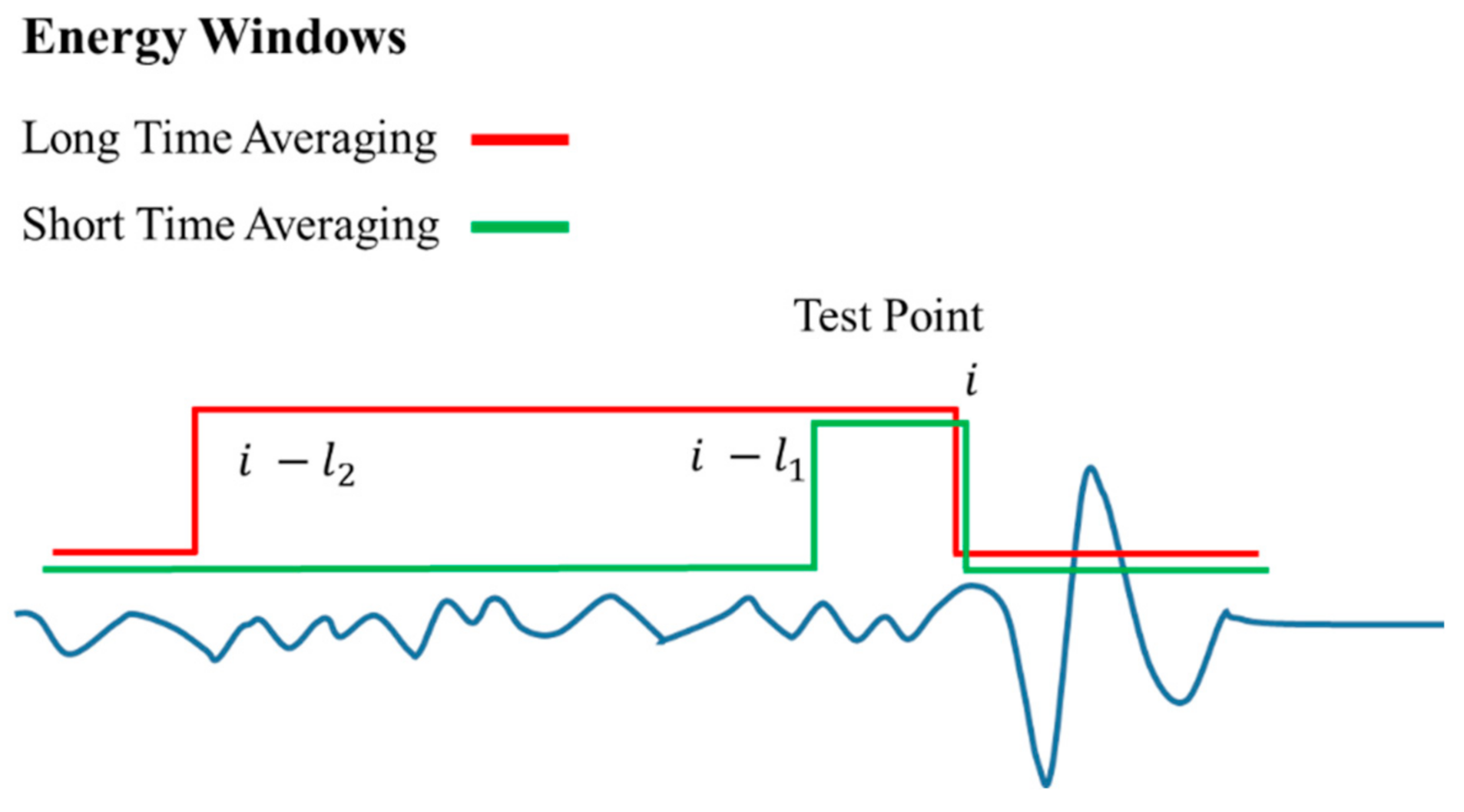
After converting raw data to miniSEED format and pre-processing including linear offset removal and normalization, the standard STA/LTA (short-time averaging/long-time averaging) algorithm was employed for signal and noise sample generation. Equations (1) and (2) and Figure 3 describes the basic concept of the short-time averaging and long-time averaging triggering method. In Equations (1) and (2) and Figure 3, i is an index of the test data point and are window-lengths of the STA and LTA. By examining the Equations and Figure, STA is literally averaging the amplitude of the short periods; thus, it reflects an abrupt amplitude change in the waveform (Equation (1) and green line in Figure 3). Conversely, LTA means the long trend of the data representing a mean energy level of noise (Equation (2) and red solid line in Figure 3). In principle, the STA/LTA ratio will increase as it approaches the P-wave onset and then decrease. Thus, the STA/LTA algorithm is commonly used for P-wave onset picking (triggered time) and event triggering as well. We used the standard STA/LTA subroutine provided in the ObsPy library [36] for already triggered events. There are precise algorithms to pick first arrival [37,38,39,40]. However, a simple STA/LTA algorithm is sufficient to work out for the purpose of dividing the data into signal and noise.
Figure 4 describes the preparation of sample data for machine learning with the triggered data in detail. We divided the time trace of sample data into the noise and signal based on the event’s triggered time. To prevent the omission of signal due to error of triggering by STA/LTA algorithm, a 0.1 s before the triggered time calculated from the STA/LTA algorithm was used as a triggered time.
During observations of 2 years of the hydraulic stimulations, source–receiver distances were generally approximately less than 5 km (we assume that the average approximate P wave velocity is around 5.6 km/s and S wave velocity is around 3.294 km/s based on the sonic log on the EGS site). Regarding the residual energy after S wave arrival, an additional 1 s was enough to contain all the P and S wave characteristics. Thus, the authors decided on the 2 s window after P wave onset for the signal.
Thus, data points in a 2 s time window before the triggered time were labeled as noise. The same time window parameter was applied to the data after the triggered time, and it was labeled as a signal. In this way, we augmented the training data, which comprise 99 noise events and 99 signal events. The total number of amplitude data points was 1001, since the typical samples per second of PHBSs was 500 (i.e., 500 data points per second), where its Nyquist frequency (250 Hz) was within the actual frequency range (<200 Hz) of signals according to the spectrograms in Figure 4.
In this study, one data sample represents each of Figure 4a–i. Thus, one data sample is composed of 1001 data points. Each data point indicates an amplitude value. There were three direction measurements from one of signal or noise events. Thus, there were 3003 data points for each event. In the machine or deep learning of this study, one training data sample is composed of three data samples from the three directions, which means that there were data points for each training data sample. Data point, data sample, and training data sample should be taken as having different meanings; they are defined separately for a better understanding of data construction and convenience of labeling and training for machine learning.
2.2. Supervised Learning: Random Forest and Convolutional Neural Network
Random forest (RF) is composed of multiple decision trees. A decision tree finds the most explanatory features, which appropriately divide a given data pool such that the divided data have a higher purity than before the division [42,43]. For example, it assumes that there are training data samples as shown in Figure 5a and that they can be categorized into noise (black) and signal (red) classes as presented. The data are scattered in two dimensions: first and second features. The features could be any data point among the 3003 data points.
If all the data were organized according to the first feature, they would be arrayed as Figure 5b. A thick red bar on Figure 5b indicates a decision boundary dividing the given data into two groups. If a decision boundary was set on the second feature, it would be arrayed as in Figure 5c. In the case of the first feature, the organized data show a distributed trend in an orderly fashion in spite of the mixed training data samples. In Figure 5c, whichever criterion is fixed to classify the entire data, it will have impurity compared to Figure 5b. After Figure 5c, the two subgroups can be divided further into another two subgroups, respectively, as displayed in Figure 5d.
Figure 5e depicts how a decision tree divides the given data pool into branches. The training data samples are labeled as 0 (signal) and 1 (noise). Each sample is composed of 3003 data points. Among the 3003 data points, we find a decision boundary to separate given data into two groups having similar features, respectively, such that it has lower impurity. Including the far lower right part, Figure 5e has four stages of dividing the given data. The first, second, and third stages correspond to Figure 5a,c,d, respectively. In the far lower right of Figure 5e, there are five samples, and they are categorized into three signals (the left dotted-line circle) and two noises (the right dotted-line circle). Although the degree of purity is likely to increase by narrowing down to multiple subgroups (Figure 5e), an excessive number of branches could cause overfitting and weakened generality.
In most cases, a randomly mixed data pool has high complexity and impurity, which must show a similar condition to the low purity of Figure 5c rather than the high purity of Figure 5b. That is, there might be no features to categorize data as clearly as Figure 5b does. Thus, we should be able to solve more complicated situations such as in Figure 5c than in Figure 5b. In such a complicated situation, we are bound to encounter many scenarios corresponding to how given data are divided. Therefore, only one single decision tree could give us a biased decision, even though a decision tree has the advantages of simplicity and understandability. To avoid this drawback, multiple decision trees are trained, and they consist of one RF model.
Figure 6 schematically describes the concept of RF composed of multiple decision trees. Typically, the stability of performance increases with the greater number of decision trees; however, computational cost also increases proportionally, and hence an optimal number of trees should be fixed. Thus, although the number of trees depends on the number of data samples and features, it is usually decided as a few hundred to a few thousand [42,44,45,46,47].
CNN is one of the neural networks used for deep learning. CNN extracts the best features from data by pooling and convolution [46,48,49,50,51,52]. Figure 7 describes how pooling and convolution work during data processing. Figure 7a,b are examples of global average pooling and max pooling. Global average pooling calculates the mean of 16 values (each convolution layer of Figure 7a) and brings one averaged value as the representative of each convolution layer. Max pooling outputs maximum value from each assigned area by scanning window and stride. Here, stride is the moving step of the scanning window. The sizes of window and stride are 2-by-2 and 2, respectively, as in Figure 7b, such that this process brings four representative figures. Figure 7c is an example of convolution with a 3-by-3 kernel, 1 stride, and padding. A kernel is similar to a scanning window of max pooling, and the size or elements can be different to determine different trends of an image as shown in Figure 7d. Padding consists of supplementary grids surrounding an original input layer to preserve data size. Although the principles of pooling and convolution are different, the idea behind them is to extract essential information from a given image’s data. In general, a series of convolution or pooling layers are stacked to suitably deal with images and to achieve users’ needs such as denoising, detection, location, and classification of seismic data [48,53].
We designed CNN using AutoKeras [54], which automatically and efficiently searches for an optimal neural architecture. Schematically, the overall CNN application was constructed as shown in Figure 8. The number of data points for an axis is 1001, and there are three axes (Figure 8a). One training sample is composed of the three axes such that a sample is composed of 3003 data points in total (Figure 8a). Those with multiple samples consist of training data. As shown in Figure 8b, one sample is taken as 1001 by 1 by 3 and the last 3 means the three channels of CNN input form. In Figure 8c, CNN is constructed with convolutional layers for convolutions and poolings. Then, it is ended to a fully connected network and sigmoid [55] to give values of 0 to 1, which indicate the probability of whether it is a noise or a signal (Figure 8d).
2.3. Unsupervised Learning: K-Medoids Clustering
K-medoids is a data clustering algorithm to categorize given data into k groups with k centroids. K-means clustering, also a clustering algorithm, decides center location as averaged coordinates of each data group, k. However, the K-means algorithm has a couple of drawbacks compared to K-medoids [56,57,58]. First, it is highly dependent on the initial locations of k representative points. Second, it does not properly work for different sizes and densities of clusters. Third, it is vulnerable to noise or outliers such that the clustering result could be biased. On the other hand, K-medoids clustering gives less overlapping clustering results, is less sensitive to outliers, and is more representative of centers for each cluster. There are variant versions of the K-medoids algorithm, and this study utilizes the partitioning around medoids (PAM) [58] algorithm as outlined in the following sequence and depicted in Figure 9:
- Given training data samples are presented in the dimension of data features and randomly select k data points as the representatives (medoids) among the entire n data points (Figure 9a).
- The rest of the data points are assigned to each of the k center points when data have the closest distance from the medoids (Figure 9b).
- The locations of the medoids are changed, and the sum of within-cluster distances for before and after (Figure 9c) situations is computed.
- Medoids option showing the lower sum of within-cluster distances is selected (Figure 9c).
- Steps 2 to 4 are repeated until there is no change in the locations of the medoids.
As mentioned in Figure 4, there were 198 seismic data samples composed of 99 signal and 99 noise samples, and they were presented as one data point as described in Figure 9a. According to previous studies and experiences, the vertical component is the first data to be analyzed. The vertical component reflects the P-wave energy most clearly in many cases [59,60]. Besides, we can save computational costs by using one component rather than three components for event classification. For that reason, the vertical component was selected as the only representative feature of the 198 seismic data samples analyzed in this study. Distance (similarity–dissimilarity) between the samples is defined as Euclidean in this study as the following Equation (3):
where means covariance matrix representing relationship among the microseismic samples and a component of ith row and jth column in is Euclidean distance between ith sample and jth sample, is the number of given training samples and it comprises 198 seismic data in this study. Thus, the matrix is 198 by 198 symmetric covariance matrix with zero components on the diagonal line.
3. Results and Discussion
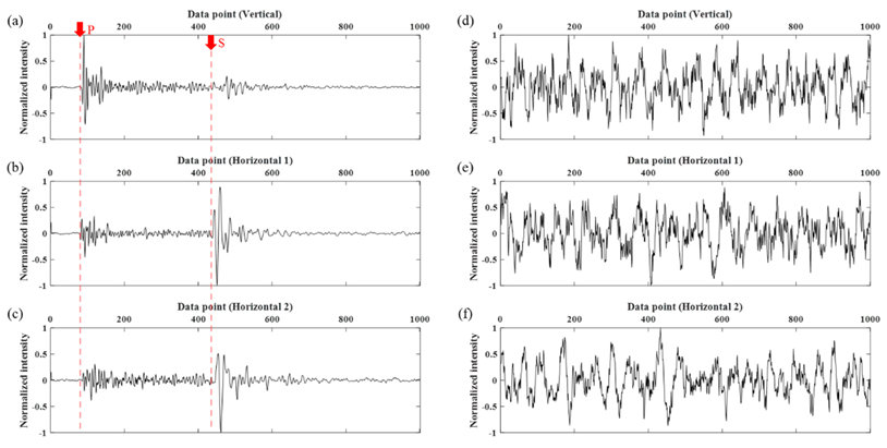
Figure 10 presents two examples of signal and noise samples, respectively. One sample consists of three directions: vertical, horizontal 1, and 2 in Figure 10a–f. The red dotted line and arrows indicate the onset time of P- and S-wave energies. In Figure 10a–c, one can clearly observe that the amplitude level is above the average amplitude level before and after the red dotted lines. The start of the P-wave is the most important feature to determine whether it is an event or not. In the middle of Figure 10a–c, S-wave energy is also clearly distinguishable. In the horizontal components, the S-wave energy is orthogonal to the P-wave vibration that was successfully detected. On the other hand, Figure 10d–f display an example of ambient noise, where the average level of the amplitude is comparably consistent with the fluctuations through all data points. For this study, the amplitude information is used directly as an input data sample for supervised and unsupervised learning. We presumed that P and S wave information is not reflected in machine learning explicitly but implicitly.
Table 1 shows the training condition for RF and CNN. For all machine learning processes, we used a workstation with an Intel Xeon Gold 6136 central processing unit using 3 and 2.99 GHz processors with 128 GB of random access memory. The number of data was 198, which was composed of 99 signal and 99 noise samples. Training data used 80% of the samples, and the test data used 20%. The size of one sample is 3003 for axes in three directions. The maximum depth for RF was set at 10 for proper classification performance. The number of trees was optimized at 200 considering affordable computation cost for less than 30 min with a stable performance regardless of randomness. In the case of CNN, its neural structure was optimized according to Auto-Keras, the automated deep learning algorithm [54]. The number of maximum epochs and the validation split ratio was decided at typical levels.
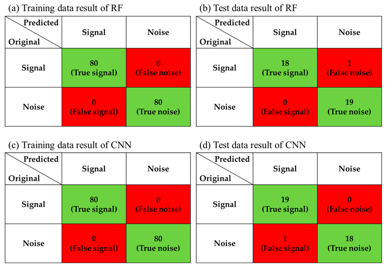
Figure 11 displays how RF and CNN predict the original microseismic data in a confusion matrix form. Green and red color indicate right and wrong prediction, respectively. Figure 11a,b are the training and test results from RF, and Figure 11c,d present those from CNN. Both RF and CNN show 100% accuracy in training results. The RF shows only one false noise, which means it is a signal that was evaluated as noise, was observed. On the other hand, CNN brings one false signal, that is, it predicted noise as signal. Although it turns out that both RF and CNN have the same accuracy of performance, the two methods must be compared from the perspective of uncertainty.
Figure 12 describes the probability of a given sample being assigned to the signal group. Both RF and CNN can output continuous probability values between 0 and 1 (0: signal, 1: noise). The RF model is composed of multiple trees, and each tree gives a bimodal result, 0 or 1. The CNN model ends with the sigmoid model giving stochastic values from 0 to 1. In Figure 12, each point indicates the probability to be a signal for each data sample in order (see Table 1). In Figure 12a,c, the training samples 1 to 80 and 81 to 160 mean noise and signal data, respectively. Accordingly, the probability values are well matched to the data distribution, which indicates that the training samples are properly categorized into signal and noise by both the RF and the CNN.
Conversely, Figure 12b shows the probability values of around 0.5, which means that those samples cause a difficulty in classification. In the case of test sample number 20 with the red circle, it should be in the signal, but it is classified as noise. The CNN model still presents clear stochastic indications to classify noise and signal in the test samples (Figure 12d). However, the test sample number 19 with the red circle, which is supposed to be noise, is wrongly classified as signal.
Figure 13 displays the false noise and false signal from the results of RF and CNN. Figure 13a–c and Figure 13d–f correspond to false noise and false signal of Figure 11b and Figure 11d, respectively. In that, the left column sample of Figure 13 is actually signal and the right one of Figure 13 is noise. The model constructed in machine learning is the black-box, and it does not explicitly provide the reason for classification, and it needs to infer what the RF and CNN models did for sample numbers 20 and 19. Thirty-eight test data samples of signals and noises (Appendix A) were thoroughly investigated.
It is hypothesized that the RF-trained model confused signal as noise because of the amplitude fluctuation pattern of the vertical component. The energy of the vertical component in Figure 13a is weak compared to the ambient noise level. For the CNN model case, we found that the overall amplitude fluctuation pattern of the vertical component from the noise samples is similar except for that of sample number 19, which has an abrupt elevation in amplitude at the end of the data points (Figure 13d). This implies that the trained CNN model might determine noise according to the vertical component and sample 19 was peculiarly patterned to be noise.
The horizontal components of noise samples have a variety of patterns compared to the vertical component. Inconsistent noise trends are similar to signal samples. Therefore, there is a good chance that the RF model and the neural structure of the CNN model assign low weights for the horizontal components compared to the vertical one because the horizontal components lack consistent features, so they are less helpful for the identification of noise.
Figure 14 shows the k-medoids clustering results of the normalized and fast Fourier transformed (FFT) samples. FFT is widely utilized to analyze waveform data such as mircroseismic from drilling, blasting, and earthquake [62,63,64]. FFT transforms given mircroseismic data from the time domain to the frequency domain such that it makes it easier to identify the specific pattern or trend, leading to reliable characterization or classification of signal and noise. The 198 training data samples were composed of 99 signal and 99 noise (Figure 14a,d). They were clustered into 10 groups indicated in the upper right corner of Figure 14a,d. Centers of each group are also marked with black empty circles. Figure 14b,c,e,f are pictured to separately show samples corresponding to each center of 10 clusters. They are put into odd and even groups to avoid overlapping.
In Figure 14a, cluster number nine is the signal group, which is indicated with green colored balls with a black edge as shown in the label. Figure 14b shows the center sample of cluster number nine, and it has a general pattern of signal (P and S waves). In Figure 14b,c, the rest of the nine center samples present an irregular noise pattern. In Figure 14d, cluster number one, the red cross marks indicate the signal group, and they also show the certain trend of P and S waves. We can manually guess whether a cluster is assigned to a signal or noise based on the 10 center samples in this study.
The fact that the clustering properly categorizes 198 samples into signal and noise is validated. Figure 15a,b show the accuracies of k-medoids clustering for the normalized and FFT samples at 89% and 97%, respectively. The difference in accuracy of 8% means that FFT helps to extract essential features of microseismic data. In the cases of the classifications by RF and CNN, there was no need to reconsider their machine learning performances because both methods were workable and affordable. In terms of the application of k-medoids on the normalized samples, 89% accuracy is insufficient for application to field data for practical purposes, and hence, FFT is the better option.
A comparison of Figure 15a,b shows that the number of false noises is 3. On the other hand, the number of false signals is reduced from 19 to 3, which is encouraging because it saves us time spent on checking false signals. In Figure 15a,b, the false noise is critical because we could miss important events by treating them as noise. Sorting out these confusing samples needs attention in a further study.
4. Conclusions
This study validated the potential of successful machine learning applicability for signal–noise classification of microseismic data from the Pohang EGS project. The seismic data presented in this study are the first and unique microseismic data obtained during the hydraulic-stimulation test for the first EGS project in Korea. The number of training data samples was 198, composed of 99 signal and 99 noise, which has an advantageous data composition of 50:50 between two classes for reliable classification performance based on machine learning.
Supervised and unsupervised learning methods were utilized to address the classification and the results showed decent accuracy. The two supervised methods (RF and CNN) brought satisfying accuracies of 100% and 97.4% for the training and test sets, respectively, in both RF and CNN. The unsupervised method, K-medoids clustering, gave 88.9% and 97.0% accuracy for the normalized data and FFT data, respectively. Generally, the classification performance seems to be sufficiently trustworthy if it would be applied for practical utilization in the field in real-time. RF worked appropriately for classification because the quality of training data was well-qualified and came from one water injection well, which must have led to consistency of the signal data.
The quantity of the utilized data might be insufficient; however, extra data would be added in the future after resolving the public acceptance problem by thorough government investigation on the EGS project after the Pohang earthquake in 2017 and contribute to further studies on the overall geological environment to understand complex fracture and fault systems present in Pohang. Therefore, this study is a suitable starting point for the processing and understanding of microseismic activities that occur after the Pohang earthquake, which still needs to be understood. Furthermore, a new project planned by KIGAM is expected to drastically improve the quantity of microseismic data. In addition, Korea Meteorological Administration and Earthquake Research Center in KIGAM are trying to install many seismometers to detect micro-earthquakes and delineate fault systems.
Accurate and fast event triggering and classification of signal and noise will be required in the immediate future as an enormous amount of data will be generated by investigations of complex fracture and fault networks. Therefore, we expect to expand the generality of the proposed method by refining using new data and continuously updating the data pool. Such recurrent application of the method will lead to the construction of the automatic process and learning system for a signal–noise classification.
Author Contributions
Conceptualization, B.Y. and S.K.; Methodology, S.K., B.Y., and J.-T.L.; Validation, S.K., J.-T.L., and B.Y.; Formal Analysis, S.K., J.-T.L., B.Y., and M.K.; Investigation, S.K., B.Y., J.-T.L., and M.K.; Writing—Original Draft Preparation, S.K. and B.Y.; Writing—Review and Editing, S.K., B.Y., and M.K.; Project Administration, B.Y. All authors have read and agreed to the published version of the manuscript.
Funding
This research was funded by the Korea Institute of Geoscience and Mineral Resources (KIGAM) grant number GP2020-025.
Acknowledgments
This study was supported by the Korea Institute of Geoscience and Mineral Resources (KIGAM) (GP2020-025). Micro-seismic data were supported by the Korea Institute of Energy Technology Evaluation and Planning (KETEP) granted financial resources from the Ministry of Trade, Industry & Energy, Republic of Korea (No. 20123010110010).
Conflicts of Interest
The authors declare no conflict of interest.
Appendix A
Figure A1.
Signal test samples (horizontal 1, horizontal 2, and vertical).

Figure A2.
Noise test samples (horizontal 1, horizontal 2, and vertical).

References
- Leake, M.R.; Conrad, W.J.; Westman, E.C.; Afrouz, S.G.; Molka, R.J. Microseismic Monitoring and Analysis of Induced Seismicity Source Mechanisms in a Retreating Room and Pillar Coal Mine in the Easter Unites States. Undergr. Space 2017, 2, 115–124. [Google Scholar] [CrossRef]
- Maxwell, S. Microseismic Imaging of Hydraulic Fracturing: Improved Engineering of Unconventional Shale Reservoirs. Soc. Explor. Geophys. 2014. [Google Scholar] [CrossRef]
- Provost, F.; Hibert, C.; Malet, J.P. Automatic Classification of Endogenous Landslide Seismicity Using the Random Forest Supervised Classifier. Geophys. Res. Lett. 2017, 44, 113–120. [Google Scholar] [CrossRef]
- Contrucci, I.; Balland, C.; Kinscher, J.; Bennani, M.; Bigarre, P.; Bernard, P. Aseismic Mining Subsidence in an Abandoned Mine: Influence Factors and Consequences for Post-Mining Risk Management. Pure Appl. Geophys. 2019, 176, 801–825. [Google Scholar] [CrossRef]
- Hong, J.S.; Lee, H.S.; Lee, D.H.; Kim, H.Y.; Choe, Y.T.; Park, Y.J. Microseismic Event Monitoring of Highly Stressed Rock Mass Around Underground Oil Storage Caverns. Tunn. Undergr. Space Technol. 2006, 21, 292. Available online: http://worldcat.org/issn/08867798 (accessed on 8 March 2021). [CrossRef]
- Lin, B.; Wei, X.; Junjie, Z. Automatic Recognition and Classification of Multi-Channel Microseismic Waveform Based on DCNN and SVM. Comput. Geosci. 2019, 123, 111–120. [Google Scholar] [CrossRef]
- Peng, P.; He, Z.; Wang, L. Automatic Classification of Microseismic Signals Based on MFCC and GMM-HMM in Underground mines. Shock Vib. 2019. [Google Scholar] [CrossRef]
- Kim, K.; Min, K.; Kim, K.; Choi, J.; Yoon, K.; Yoon, W.; Yoon, W.; Yoon, B.; Lee, T.; Song, Y. Protocol for Induced Microseismicity in the First Enhanced Geothermal Systems Project in Pohang, Korea. Renew. Sustain. Energy Rev. 2018, 91, 1182–1191. [Google Scholar] [CrossRef]
- The Definition of Micro-Earthquake. Available online: https://en.wikipedia.org/wiki/Microearthquake (accessed on 25 February 2021).
- Kwiatek, G.; Saarno, T.; Ader, T.; Bluemle, F.; Bohnhoff, M.; Chendorain, M.; Dresen, G.H.; Kukkonen, I.; Leary, P.; Leonhardt, M. Controlling Fluid-Induced Seismicity During a 6.1-km-Deep Geothermal Stimulation in Finland. Sci. Adv. 2019, 5, 7224. [Google Scholar] [CrossRef] [Green Version]
- Wilks, M.; Wuestefeld, A.; Oye, V.; Thomas, P.; Kolltveit, E. Tailoring Distributed Acoustic Sensing Techniques for the Microseismic Monitoring of Future CCS Sites: Results from the Field. In SEG Technical Program Expanded Abstracts, Proceedings of the SEG International Exhibition and 87th Annual Meeting, Houston, TX, USA, 23 October 2017; Society of Exploration Geophysicists: Houston, TX, USA, 2017; pp. 2762–2766. [Google Scholar] [CrossRef]
- Wang, H.; Li, M.; Shang, X. Current Developments on Micro-Seismic Data Processing. J. Nat. Gas. Sci. Eng. 2016, 32, 521–537. [Google Scholar] [CrossRef]
- Pan, S.; Qin, Z.; Lan, H.; Badal, J. Automatic First-Arrival Picking Method Based on an Image Connectivity Algorithm and Multiple Time Windows. Comput. Geosci. 2019, 123, 95–102. [Google Scholar] [CrossRef] [Green Version]
- Chamberlain, C.J.; Hopp, C.J.; Boese, C.M.; Warren-Smith, E.; Chambers, D.; Chu, S.X.; Michailos, K.; Townend, J. EQcorrscan: Repeating and Near-Repeating Earthquake Detection and Analysis in Python. Seismol. Res. Lett. 2018, 89, 173–181. [Google Scholar] [CrossRef]
- Lin, B.; Wei, X.; Junjie, Z.; Hui, Z. Automatic Classification of Multi-Channel Microseismic Waveform Based on DCNN-SPP. J. Appl. Geophys. 2018, 159, 446–452. [Google Scholar] [CrossRef]
- Miao, F.; Carpenter, N.S.; Wang, Z.; Holcomb, A.S.; Woolery, E.W. High-Accuracy Discrimination of Blasts and Earthquakes Using Neural Networks with Multiwindow Spectral Data. Seismol. Res. Lett. 2020, 91, 1646–1659. [Google Scholar] [CrossRef]
- Sertcelik, F.; Yavuz, E.; Birdem, M.; Merter, G. Discrimination of the Natural and Artificial Quakes in the Eastern Marmara region, Turkey. Acta Geod. Geophys. 2020, 55, 645–665. [Google Scholar] [CrossRef]
- KIGAM. Characteristic Analysis and Library Buildup for Microseismic Signals Originated by Mining Activities; Report GP2018-001-2019; Inha University: Daejeon, Korea, 2019; p. 51. [Google Scholar]
- Kislov, K.V.; Gravirov, V.V. Use of Artificial Neural Networks for Classification of Noisy Seismic Signals. Seism. Instrum. 2017, 53, 87–101. [Google Scholar] [CrossRef]
- Ross, Z.E.; Meier, M.A.; Hauksson, E.; Heaton, T.H. Generalized Seismic Phase Detection with Deep Learning. Bull. Seismol. Soc. Am. 2018, 108, 2894–2901. [Google Scholar] [CrossRef] [Green Version]
- Ross, Z.E.; Meier, M.A.; Hauksson, E. P Wave Arrival Picking and First-Motion Polarity Determination with Deep Learning. J. Geophys. Res. Solid Earth 2018, 123, 5120–5129. [Google Scholar] [CrossRef]
- Bergen, K.J.; Johnson, P.A.; Maarten, V.; Beroza, G.C. Machine Learning for Data-Driven Discovery. Solid Earth Geosci. Sci. 2019, 363, 323. [Google Scholar] [CrossRef]
- Kong, Q.; Trugman, D.T.; Ross, Z.E.; Bianco, M.J.; Meade, B.J.; Gerstoft, P. Machine Learning in Seismology: Turning data into insights. Seismol. Res. Lett. 2019, 90, 3–14. [Google Scholar] [CrossRef] [Green Version]
- Linville, L.; Pankow, K.; Draelos, T. Deep Learning Models Augment Analyst Decisions for Event Discrimination. Geophys. Res. Lett. 2019, 46, 3643–3651. [Google Scholar] [CrossRef]
- Nakano, M.; Sugiyama, D.; Hori, T.; Kuwatani, T.; Tsuboi, S. Discrimination of Seismic Signals from Earthquakes and Tectonic Tremor by Applying Convolutional Neural Network to Running Spectral Images. Seismol. Res. Lett. 2019, 90, 530–538. [Google Scholar] [CrossRef]
- Rojas, O.O.; Alvarado, L.; Mus, S.; Tous, R.T. Artificial Neural Networks as Emerging Tools for Earthquake Detection. Comput. Sist. 2019, 23, 335–350. [Google Scholar] [CrossRef]
- Foody, G.M.; Pal, M.; Rocchini, D.; Garzon-Lopez, C.X.; Bastin, L. The Sensitivity of Mapping Methods to Reference Data Quality: Training Supervised Image Classifications with Imperfect Reference Data. Int. J. Geo-Inf. 2016, 5, 199. [Google Scholar] [CrossRef] [Green Version]
- Korean Government Commission. Final Report of the Korean Government Commission on Relations between the 2017 Pohang Earthquake and EGS Project; Technical Report; The Geological Society of Korea: Seoul, Korea, 2019. [Google Scholar]
- Woo, J.U.; Kim, M.; Sheen, D.H.; Kang, T.S.; Rhie, J.; Grigoli, F.; Ellsworth, W.L.; Giardini, D. An in-depth Seismological Analysis Revealing a Causal Link Between the 2017 MW 5.5 Pohang Earthquake and EGS Project. J. Geophys. Res. Solid Earth 2019, 124, 13060–13078. [Google Scholar] [CrossRef] [Green Version]
- Park, S.; Kim, K.I.; Xie, L.; Yoo, H.; Min, K.B.; Kim, M.; Yoon, B.; Kim, K.Y.; Zimmermann, G.; Guinot, F.; et al. Observations and Analyses of the First Two Hydraulic Stimulations in the Pohang Geothermal Development Site, South Korea. Geothermics 2020, 88. [Google Scholar] [CrossRef]
- Song, Y.; Lee, T.; Jeon, J.; Yoon, W. Background and Progress of the Korea EGS Pilot Project. In Proceedings of the WGC (World Geothermal Congress), Melbourne, Australia, 19–25 April 2015. [Google Scholar]
- Sohn, Y.K.; Rhee, C.W.; Shon, H. Revised Stratigraphy and Reinterpretation of the Miocene Pohang Basinfill, SE Korea: Sequence Development in Response to Tectonism and Eustasy in a Back-Arc Basin Margin. Sediment. Geol. 2001, 143, 265–285. [Google Scholar] [CrossRef]
- Trnkoczy, A.; Bormann, P.; Hanka, W.; Holcomb, L.G.; Nigbor, R.L. Site Selection, Preparation and Installation of Seismic Stations. In New Manual of Seismological Observatory Practice (NMSOP); Deutsches GeoForschungsZentrum GFZ: Potsdam, Germany, 2009; pp. 1–108. [Google Scholar]
- Lee, T.; Song, Y.; Park, D.; Jeon, J.; Yoon, W. Three-Dimensional Geological Model of Pohang EGS Pilot Site, Korea. In Proceedings of the WGC (World Geothermal Congress), Melbourne, Australia, 19–25 April 2015. [Google Scholar]
- InStie Software. Available online: https://www.itascainternational.com/software/InSite-Geo (accessed on 17 February 2021).
- Beyreuther, M.; Barsch, R.; Krischer, L.; Megies, T.; Behr, Y.; Wassermann, J. ObsPy: A Python toolbox for seismology. Seismol. Res. Lett. 2010, 81, 530–533. [Google Scholar] [CrossRef] [Green Version]
- Baer, M.; Kradolfer, U. An Automatic Phase Picker for Local and Teleseismic Events. Bull. Seismol. Soc. Am. 1987, 77, 1437–1445. [Google Scholar]
- Withers, M.; Aster, R.; Young, C.; Beiriger, J.; Harris, M.; Moore, S.; Trujillo, J. A Comparison of Select Trigger Algorithms for Automated Global Seismic Phase and Event Detection. Bull. Seismol. Soc. Am. 1998, 88, 95–106. [Google Scholar]
- Akazawa, T. A Technique for Automatic Detection of Onset Time of P-and S-Phases in Strong Motion Records. In Proceedings of the 13th World Conference on Earthquake Engineering, Vancouver, BC, Canada, 1–6 August 2004. [Google Scholar]
- Havskov, J.; Ottemoller, L. Routine Data Processing in Earthquake Seismology: With Sample Data, Exercises, and Software; Springer: Dordrecht, The Netherlands, 2010. [Google Scholar] [CrossRef]
- Han, L.; Wong, J.; Bancroft, J.C. Time Picking and Random Noise Reduction on Microseismic Data. CREWES Res. Rep. 2009, 21, 1–13. [Google Scholar]
- Breiman, L. Random Forests. Mach. Learn. 2001, 45, 5–32. [Google Scholar] [CrossRef] [Green Version]
- Kim, S.; Lee, K.; Lee, M.; Ahn, T.; Lee, J. Data-Driven Three-Phase Saturations Identification from X-ray CT Images with Critical gas Hydrate Saturation. Energies 2020, 13, 5844. [Google Scholar] [CrossRef]
- Dong, L.; Li, X.; Xie, G. Nonlinear Methodologies for Identifying Seismic Event and Nuclear Explosion Using Random Forest, Support Vector Machine, and Naive Bayes Classification. Abstr. Appl. Anal. 2014, 459137. [Google Scholar] [CrossRef] [Green Version]
- Hibert, C.; Provost, F.; Malet, J.P.; Maggi, A.; Stumpf, A.; Ferrazzini, V. Automatic Identification of Rockfalls and Volcano-tectonic Earthquakes at the Piton de la Fournaise Volcano Using a Random Forest Algorithm. J. Volcanol. Geotherm. 2017, 340, 130–142. [Google Scholar] [CrossRef]
- Kim, S.; Lee, K.; Lee, M.; Ahn, T.; Lee, J.; Suk, H.; Ning, F. Saturation Modeling of Gas Hydrate Using Machine Learning with X-ray CT Images. Energies 2020, 13, 5032. [Google Scholar] [CrossRef]
- Kim, T.; Kim, S.; Lim, J. Modeling and Prediction of Slug Characteristics Utilizing Data-Driven Machine-Learning Methodology. J. Petrol. Sci. Eng. 2020, 195, 107712. [Google Scholar] [CrossRef]
- Huang, L.; Li, J.; Hao, H.; Li, X. Micro-Seismic Event Detection and Location in Underground Mines by Using Convolutional Neural Networks (CNN) and Deep Learning. Tunn. Undergr. Space Technol. 2018, 81, 265–276. [Google Scholar] [CrossRef]
- Such, F.P.; Peri, D.; Brockler, F.; Hutkowski, P.; Ptucha, R.; Alaris, K. Fully Convolutional Networks for Handwriting Recognition. In Proceedings of the 2018 16th International Conference on Frontiers in Handwriting Recognition (ICFHR), Niagara Falls, NY, USA, 5–8 August 2018; pp. 86–91. [Google Scholar] [CrossRef] [Green Version]
- Chu, M.; Min, B.; Kwon, S.; Park, G.; Kim, S.; Huy, N.X. Determination of an Infill Well Placement Using a Data-Driven Multi-modal Convolutional Neural Network. J. Petrol. Sci. Eng. 2020, 195, 106805. [Google Scholar] [CrossRef]
- Cunha, A.; Pochet, A.; Lopes, H.; Gattass, M. Seismic Fault Detection in Real Data Using Transfer Learning from a Convolutional Neural Network Pre-trained with Synthetic Seismic Data. Comput. Geosci. 2020, 135, 104344. [Google Scholar] [CrossRef]
- Kim, S.; Lee, K.; Lim, J.; Jeong, H.; Min, B. Development of Ensemble Smoother-Neural Network and its Application to History Matching of Channelized Reservoir. J. Petrol. Sci. Eng. 2020, 191, 107159. [Google Scholar] [CrossRef]
- Mandelli, S.; Lipari, V.; Bestagini, P.; Tubaro, S. Interpolation and Denoising of Seismic Data Using Convolutional Neural Network. arXiv 2019, arXiv:1901.07927. [Google Scholar]
- Jin, H.; Song, Q.; Hu, X. Auto-Keras: An Efficient Neural Architecture Search System. In Proceedings of the KDD’19: 25th ACM SIGKDD International Conference on Knowledge Discovery & Data Mining Anchorage, Anchorage, AK, USA, 4–8 August 2019; pp. 1946–1956. [Google Scholar] [CrossRef] [Green Version]
- Goodfellow, I.; Bengio, Y.; Courville, A. Deep Learning; MIT Press: Cambridge, UK, 2016; Volume 2, pp. 180–184. [Google Scholar]
- Park, H.S.; Jun, C.H. A Simple and Fast Algorithm for K-Medoids Clustering. Expert Syst. Appl. 2009, 36, 3336–3341. [Google Scholar] [CrossRef]
- Arora, P.; Deepali, D.; Varshney, S. Analysis of K-Means and K-Medoids Algorithm for Big Data. Procedia Comput. Sci. 2016, 78, 507–512. [Google Scholar] [CrossRef] [Green Version]
- Budiaji, W.; Leisch, F. Simple K-Medoids Partitioning Algorithm for Mixed Variable Data. Algorithms 2019, 12, 177. [Google Scholar] [CrossRef] [Green Version]
- Shearer, P.M. Introduction to Seismology; Cambridge University Press: Cambridge, UK, 2009; ISBN 0-521-88210-1. [Google Scholar]
- Chopra, A.K. The Importance of the Vertical Component of Earthquake Motions. Bull. Seismol. Soc. Am. 1966, 56, 1163–1175. [Google Scholar]
- Kang, B.; Kim, S.; Jung, H.; Choe, J.; Lee, K. Efficient Aassessment of Reservoir Uncertainty Using Distance-Based Clustering: A review. Energies 2019, 12, 1859. [Google Scholar] [CrossRef] [Green Version]
- Kumar, C.V.; Vardhan, H.; Murthy, C.S.N.; Karmakar, N.C. Estimating Rock Properties Using Sound Dominant Frequencies During Diamond Core Drilling Operations. J. Rock Mech. Geotech. Eng. 2019, 11, 850–859. [Google Scholar] [CrossRef]
- Liang, Z.; Xue, R.; Xu, N.; Li, W. Characterizing Rockbursts and Analysis on Frequency-Spectrum Evolutionary Law of Rockburst Precursor Based on Microseismic Monitoring. Tunn. Undergr. Space Technol. 2020, 105, 103564. [Google Scholar] [CrossRef]
- Li, B.; Wang, E.; Li, Z.; Niu, Y.; Li, N.; Li, X. Discrimination of Different Blasting and Mine Microseismic Waveforms Using FFT, SPWVD and Multifractal Method. Environ. Earth Sci. 2021, 80. [Google Scholar] [CrossRef]
Figure 1.
(a) PX-1 log of the Pohang enhanced geothermal system (EGS) site (modified after [34]); (b) the geometry of microseismic monitoring network for the EGS project. White squares and circles are shallow borehole stations named PHBSs (Pohang borehole stations) and temporal surface seismometers named MSS (mobile surface station), respectively. Deep borehole sensors such as Avalon GeochainTM Slim Receivers, which were originally used for vertical seismic profiling, were operated in the EGS site to improve the accuracy of the microseismic analysis in the stimulation periods; (c) the actual photographs of PHBSs and 3-axis borehole accelerometer.

Figure 2.
Pre-processing procedure of microseismic data for machine learning.

Figure 3.
The conceptual representation of short-time averaging (STA) and long-time averaging (LTA) triggering method (modified from [41]).
Figure 3.
The conceptual representation of short-time averaging (STA) and long-time averaging (LTA) triggering method (modified from [41]).

Figure 4.
The example of the PHBS8 data and their time-frequency spectrograms: vertical, horizontal 1, and horizontal 2 in order from top to bottom. (a–c) Noise and (d–f) signal examples generated from the same microseismic event. In this study, noise and signal are labeled with 1 and 0, respectively, which means the closer to 0 an output of machine or deep learning, the higher its possibility to be signal. (g–i) show spectrograms of each vertical, horizontal 1, and horizontal 2, which shows the actual frequency range of (a–f) The microseismic data was split into noise and signal based on the 0.1 s before P-wave onset time calculated from the STA/LTA algorithm. The total length of the data was 2 s; thus, 1001 data points were generated under the acquisition condition of 500 data points per second.

Figure 5.
Schematic of data classification according to features and the example of a decision tree. (a) The entire data pool with 10 samples in two classes; (b) organized data array according to the first feature showing high purity; (c) organized data array by the second feature showing comparatively less purity; (d) extra categorization into subgroups; (e) schematic of a decision tree with four stages.

Figure 6.
Schematic of random forest composed of multiple decision trees. (a) Multiple decision trees with different kinds of scenarios; (b) multiple decisions according to the trees; (c) final decision based on majority voting [42,46,47].

Figure 7.
Examples of global average pooling, max pooling, and convolution. (a) Global average pooling gives averaged values of all the elements of convolution layers; (b) max pooling selects out the maximum value from designated areas according to window and stride; (c) convolution scans input layer with a kernel window; (d) kernel windows have different elements for each pixel to extract different patterns from a given input layer.

Figure 8.
Schematic of CNN applied to seismic data with convolutional and fully connected layers for classification of noise and signal. (a) Training data of noise and signal from the three axes: the horizontal 1, 2, and vertical direction; (b) 1001 data points from each direction through the three channels as input data; (c) convolution and pooling layers for feature extraction; (d) the end of the neural network with fully connected layer and sigmoid to output between 0 and 1, indicating probability for classification.

Figure 9.
Example of K-medoids clustering application for 21 data points with two clusters. (a) Random selection of two medoids; (b) data categorization according to the two medoids; (c) updated location of the two medoids.
Figure 9.
Example of K-medoids clustering application for 21 data points with two clusters. (a) Random selection of two medoids; (b) data categorization according to the two medoids; (c) updated location of the two medoids.

Figure 10.
Normalized microseismic data for vertical and horizontal directions in the second (a–c) signal and (d–f) noise sample.
Figure 10.
Normalized microseismic data for vertical and horizontal directions in the second (a–c) signal and (d–f) noise sample.

Figure 11.
Learning results of training and test data sets by (a,b) random forest (RF) and (c,d) convolutional neural network (CNN). The top line means predicted classification from the machine learning model, and the far-left line is the original class. The green highlighted area indicates that the original class is matched to the predicted one and the red highlighted area means that the prediction fails to match the original class.

Figure 12.
Probability of being signal in training and test samples by the trained RF and CNN. (a,b) are 160 training samples and 38 test samples from RF; (c,d) are 160 training samples and 38 test samples from CNN.
Figure 12.
Probability of being signal in training and test samples by the trained RF and CNN. (a,b) are 160 training samples and 38 test samples from RF; (c,d) are 160 training samples and 38 test samples from CNN.

Figure 13.
False noise and false signal of the test set from (a–c) RF and (d–f) CNN, respectively.

Figure 14.
Clustered results of (a–c) the normalized and (d–f) fast Fourier transformed (FFT) data by k-medoids and cluster representative samples.
Figure 14.
Clustered results of (a–c) the normalized and (d–f) fast Fourier transformed (FFT) data by k-medoids and cluster representative samples.

Figure 15.
The clustering results of (a) the normalized and (b) the FFT data by K-medoids.


Table 1.
Conditions for training of RF and CNN.
| Parameters | Conditions | |
|---|---|---|
| Entire data | 198 (Signal 99 + Noise 99) | |
| Training data | 160 (Signal 1–80 + Noise 1–80) | |
| Test data | 38 (Signal 81–99 + Noise 81–99) | |
| Size of one sample | 3003 (1001 points for each of the three axes) | |
| RF | Maximum depth | 10 |
| Number of trees | 200 | |
| Number of properties | 55 | |
| CNN | Optimization | Automated deep learning by Auto-Keras |
| Maximum epochs | 300 | |
| Validation split | 20% | |
Publisher’s Note: MDPI stays neutral with regard to jurisdictional claims in published maps and institutional affiliations. |
© 2021 by the authors. Licensee MDPI, Basel, Switzerland. This article is an open access article distributed under the terms and conditions of the Creative Commons Attribution (CC BY) license (http://creativecommons.org/licenses/by/4.0/).
Share and Cite
MDPI and ACS Style
Kim, S.; Yoon, B.; Lim, J.-T.; Kim, M. Data-Driven Signal–Noise Classification for Microseismic Data Using Machine Learning. Energies 2021, 14, 1499. https://0-doi-org.brum.beds.ac.uk/10.3390/en14051499
AMA Style
Kim S, Yoon B, Lim J-T, Kim M. Data-Driven Signal–Noise Classification for Microseismic Data Using Machine Learning. Energies. 2021; 14(5):1499. https://0-doi-org.brum.beds.ac.uk/10.3390/en14051499
Chicago/Turabian StyleKim, Sungil, Byungjoon Yoon, Jung-Tek Lim, and Myungsun Kim. 2021. "Data-Driven Signal–Noise Classification for Microseismic Data Using Machine Learning" Energies 14, no. 5: 1499. https://0-doi-org.brum.beds.ac.uk/10.3390/en14051499
Note that from the first issue of 2016, this journal uses article numbers instead of page numbers. See further details here.