Feasibility of Black-Box Time Domain Modeling of Single-Phase Photovoltaic Inverters Using Artificial Neural Networks

Abstract

This paper introduces a new black-box approach for time domain modeling of commercially available single-phase photovoltaic (PV) inverters in low voltage networks. An artificial neural network is used as a nonlinear autoregressive exogenous model to represent the steady state behavior as well as dynamic changes of the PV inverter in the frequency range up to 2 kHz. The data for the training and the validation are generated by laboratory measurements of a commercially available inverter for low power applications, i.e., 4.6 kW. The state of the art modeling approaches are explained and the constraints are addressed. The appropriate set of data for training is proposed and the results show the suitability of the trained network as a black-box model in time domain. Such models are required, i.e., for dynamic simulations since they are able to represent the transition between two steady states, which is not possible with classical frequency-domain models (i.e., Norton models). The demonstrated results show that the trained model is able to represent the transition between two steady states and furthermore reflect the frequency coupling characteristic of the grid-side current.

1. Introduction

To pursue the climate goals, a trend from central power generation with a small number of large power generators to a large number of small power generators, such as wind turbines and photovoltaics (PV) can be observed [1]. In medium voltage (MV) networks and high voltage (HV) networks, large wind parks and PV power plants are connected to the network at one Point of Common Coupling (PCC). In low voltage (LV) networks, a large number of small generators are connected directly to the network at individual Points of Connection (PoCs). Plant operators of large power plants connected to MV and HV networks are responsible for the correct functionality and interaction of the individual parts (i.e., generating units) of their plant and possible adverse behavior is usually resolved by the plant operator or bilaterally between the plant operator and the utility. In LV networks, many devices owned by different users interact between each other and with the network, which can noticeably affect the correct operation of the whole LV network. In particular the high demand for PV leads to a large diversity of PV inverters of different manufacturers that result in a large diversity of individual behavior of these inverters (e.g., [2]). The inverter is the main component of the entire PV system when considering the connection to the power grid.

The design of an inverter in terms of the software implementation and the hardware has a significant impact on the non-ideal behavior, i.e., the distortion, of the injected current at the PoC. The injected current leads to a voltage drop across the network impedance and consequently causes a distorted voltage [3], which in turn affects other devices that are connected to the network. This interaction can cause major issues in terms of stability, especially in the frequency range below 2 kHz, where an interaction of the inverter control with grid resonances is possible [4]. The first known issues have occurred in the power grid of the Swiss railway where interactions of converters have led to a shutdown of the locomotives [5]. With respect to PV, shut downs of inverters have similarly been reported in the past, e.g., [6,7]. Further observed effects of the interaction of PV inverters and distribution systems are unwanted tripping [8] and the impact of resonances, e.g., [9]. Since in future the electrical power generation is expected to be dominated by renewables, these interactions will not only be important for the grid-connected devices but also for the stability of the network itself.

To analyze these interactions, suitable models are required. Typically, the manufacturers do not disclose the hardware and software components and their parameters. Therefore, the white-box approach is not applicable for system stability studies by distribution system operators (DSO). One of the major challenges is the constraints of the model structure of state of the art models and their analysis. No detailed studies on time domain black-box models are known, which can represent the critical frequency range between fundamental frequency (i.e., 50 Hz) and some kilohertz (i.e., the bandwidth of the control). Approaches for formal black-box stability analyses in frequency domain have been developed, e.g., in terms of the impedance-based stability criterion [10] or the generalized Nyquist [11]. The challenge of determining the network impedance can, e.g., be solved by probabilistic means [12]. These formal stability analyses can identify the stability qualitatively. However, to simulate the time domain characteristic of the dynamic interaction of the PV inverters with the LV network for quantitative studies requires respective black box models in time domain.

This article uses artificial neural networks (ANN) to overcome the above-mentioned constraints of the state of the art models for single-phase PV inverters for low power applications, e.g., up to 4.6 kW. The use of ANNs has been proposed in previous work, e.g., for impedance estimations in power electronic (PE) systems by recurrent neural networks (RNN) [13]. In terms of device modeling, the Hammerstein-Wiener (HW) model ([14,15,16]) has been introduced for which an ANN has been integrated to represent the nonlinear model part within the HW model. Though the HW model can be used as a time domain model, as of yet it is not able to represent frequency coupling components in the spectrum of grid-side inverter current and has not been studied for transitions between different steady states.

Furthermore, ANNs have been used to parametrize a given filter structure and a given control [17]. This approach requires knowledge about the structure of the device and is consequently no black-box approach. Modeling entire PE devices with an ANN has not been studied until now [18].

Consequently, the article develops the theoretical basis for black-box models exclusively linked to time domain. This enables the models to be used in time domain studies (e.g., electromagnetic transient (EMT) simulations). A structured procedure to train ANNs by considering the operating principle of PV inverters in LV networks is provided. For the studied and trained operating point, the ANN is able to accurately reflect the grid-side inverter current in steady state. Furthermore, it is shown that the model is able to change from one to another steady state with regard to the trained conditions. The selection of the data for training and validation as well as a suitable topology of the ANN, and a nonlinear autoregressive exogenous mode (NARX), are described. The individual structure parameters, e.g., the number of neurons, their activation function the number of layers as well as the optimization algorithm have been varied systematically to optimize the ANN.

The paper is structured as follows: In Section 2, the overall system model is explained and an overview of state of the art modeling of PV inverters is presented in Section 3. Section 4 introduces the ANN in detail, while Section 5 demonstrates the application. Section 6 discusses further aspects and finally, in Section 7, a conclusion and future work is proposed.

2. System Model

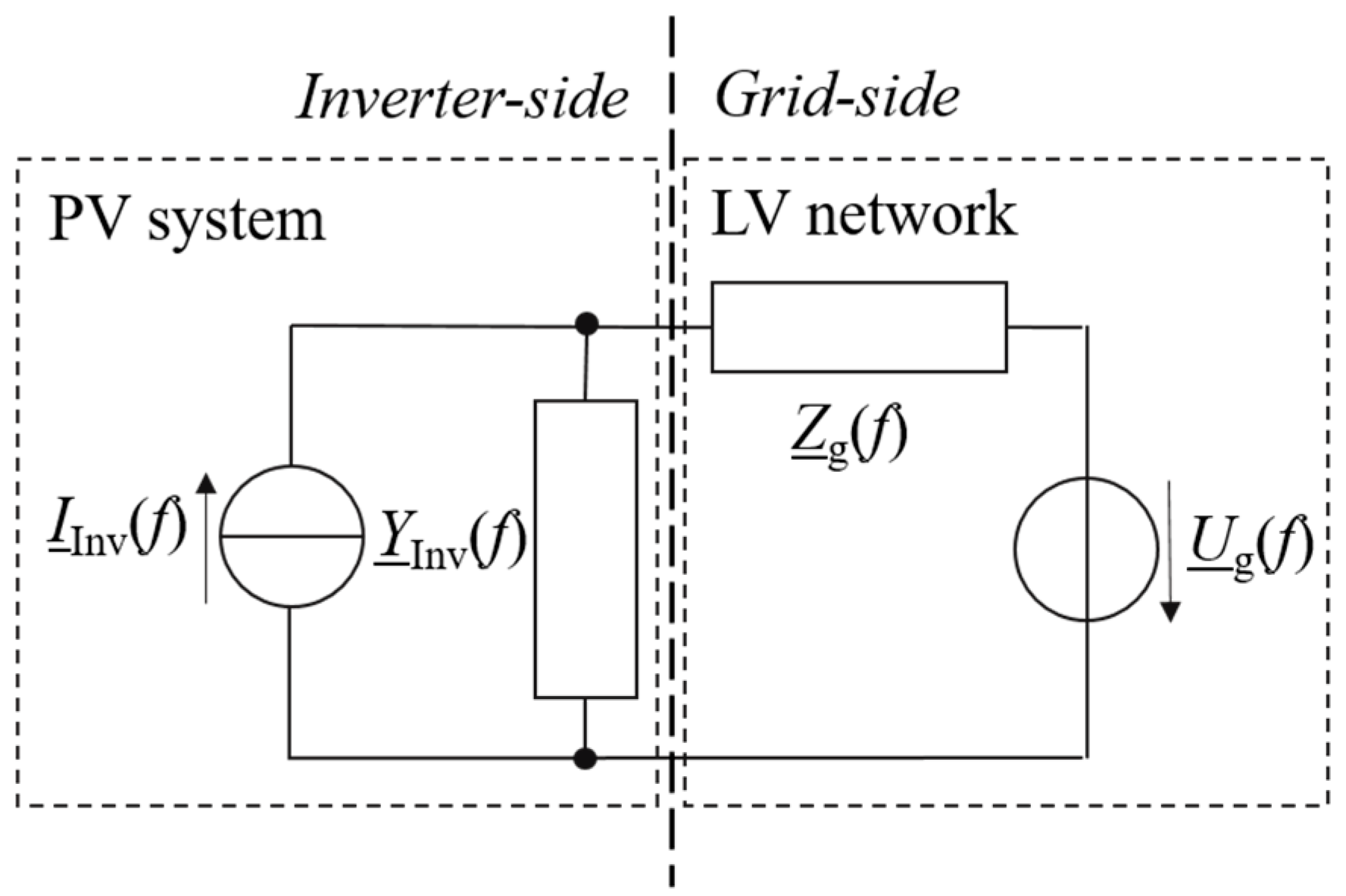
The system can be separated into the LV network and the grid-connected application, in the case of this study a PV system. Figure 1 shows an impedance-based model of a PV system and the LV network in frequency domain.

The LV network is represented by a network impedance Z_g and a voltage source. The network impedance contains the aggregated passive components that can be linearized, i.e., a proportionality between voltage and current. The active and nonlinear behavior of grid-connected devices, e.g., generators and consumers are reflected by the voltage source that represents the background voltage U_g with a background distortion. This distortion can have different origins, e.g., the impact of control algorithms on the grid-side current of PE devices, switching operations of equipment or hysteresis effects.

While the overall PV system consists of multiple components, the focus of this study is on the inverter since it is the relevant component when evaluating the interactions with the LV network. The inverter itself can be categorized into hardware components, i.e., physical elements such as resistors, inductors, capacitances and semiconductor switches, and software components, e.g., the control with the Phase locked loop (PLL), a Maximum Power Point Tracker (MPPT) and auxiliary services such as anti-islanding (AI) detection.

3. Modeling Approaches

To develop adequate models for individual study objectives, e.g., harmonic power flow studies and stability analysis, different approaches are applied with respect to the available knowledge in terms of white-box, grey-box and black box approaches.

3.1. White-Box Approach

For the white-box approach, detailed knowledge about the internal components and their parameters has to be available. If the components are known, e.g., from the manufacturer themselves, sophisticated studies of an individual inverter can be performed very accurately. The effort for the detailed implementation when studying multiple different inverters can be reduced by using a modular modeling approach [19]. However, the required computational power and convergence constraints limit the application of white-box approaches to smaller studies and they are not suitable for system studies of LV networks.

3.2. Grey-Box Approach

The grey-box approach makes use of partial knowledge about the system and includes it in the model. This approach has not received a lot of attraction and has mostly been used in terms of estimating parameters of known topologies, e.g., [17,20]. Identification methods of individual inverter components with unknown topologies have not been applied so far. Especially the identification of the control system and its nonlinearities is a major challenge.

3.3. Black-Box Approach

The black-box approach is applied if the information about the internal components and parameters of the inverter is not available. A typical representation of PV inverters consists of the decoupled Norton model, which is represented by a current source in parallel to an admittance Y_Inv (Figure 1) or the more advanced coupled Norton model that can also reflect the frequency couplings between voltage and current at different frequencies. The Hammerstein–Wiener model has also been studied for the feasibility as a black-box model structure [16], but still faces major challenges to reflect the frequency coupling appropriately. Frequency coupling implies that a single-frequent excitation at the system input leads to a multi-frequent system output. This frequency coupling can be identified by using the method of a frequency sweep according to [11], which is also the base of the more so-called fingerprint introduced in [21].

3.4. Present Modeling Constraints

3.4.1. Frequency Time Resolution

An admittance model in frequency domain as state of the art for harmonic studies in steady-state represents always a dependency of a current on a voltage. The frequency coupling components are related to the fundamental frequency of the system in terms of a specific periodicity for linear time periodic (LTP) systems. In time domain, the instantaneous values of voltage and current are defined by the time instant related to the zero crossing of the fundamental frequency of the system. However, by transforming the time domain data into frequency domain, the information about the momentary time instant, i.e., the momentary phase angle, is lost and the system is considered for the whole time duration. This challenges predictions of the output signal for frequency-domain models when the system performs a change of the steady state. Any time–frequency or frequency–time transformation and consequently the resulting time domain or frequency domain representation is subjected to the principle of uncertainty that is known under the Heisenberg–Gabor limit [22]. With the standard deviations ${\sigma }_t$ in time domain and ${\sigma }_f$ in frequency domain,

$${\sigma }_t{\sigma }_f\ge \frac{1}{4\pi }$$

(1)

states that the product of time duration and bandwidth is constant. If a frequency component is changed, the frequency that is changed and the moment when the change occurs cannot be detected at the same time. Consequently, a blurring in time–frequency resolution occurs that is called the uncertainty.

3.4.2. Implementation of System Dynamics in Simulations

Fitting algorithms are currently used to calculate RLC-elements that estimate the linear elements of the admittance matrix [23] while a current source represents the active parts and is defined by an amplitude, a phase angle and a frequency. This kind of black-box model can be used for large-scale steady state harmonic studies, but they are not intended and not able to reflect the dynamics of the PV inverter. Furthermore, the identified RLC-circuit cannot represent the frequency coupling. If the frequency coupling shall be considered, the respective current response is implemented as a constant periodic component in the current of the current source.

Load fluctuations or switching events within the simulation require an approach for the simulation that properly represents the dynamic interaction of the power grid and the inverter during the transition between two steady states or in case of an instable inverter operation. Of course, appropriate time domain models can solve this. However, accurate time domain models require detailed knowledge about the inverter, i.e., as white-box models, though this knowledge is typically not disclosed by the manufacturer. Furthermore, the computational effort is very high, because of the detailed representation, so that the number of studied devices within on simulation is restricted to only few devices. Therefore, they are not suitable for large-scale grid-studies.

3.4.3. Solver Convergence

The method using a frequency coupling matrix consisting of complex values is only suitable to derive steady state models for systems that can be linearized as typically for small signal analysis in frequency domain, e.g., harmonic power flow studies. Scenarios with expected instable device behavior run into convergence problems of the solvers if the required boundary conditions, e.g., [24,25], are not fulfilled. Thus far, it has been a challenge to prove that the convergence issue occurs due to the instable device behavior and is not caused by an inappropriate solver implementation or rather the solver settings.

4. Artificial Neural Networks

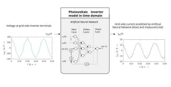
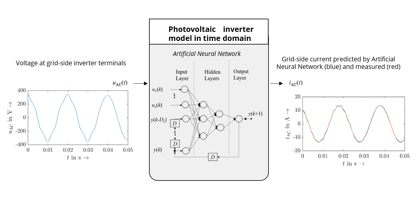
With respect to the underlying theory of dynamic interactions of the PV inverter with the LV network, a new time domain model for black-box analysis based on ANN is proposed in this study that has the potential to overcome the challenges of dynamic black-box modeling. No other measurement-based time-domain black-box models are known to the authors so far. As described previously, PV inverters consist of a complex structure compared to simplified representations, e.g., impedance-based models. As explained previously, these simplified representations cannot reflect the dynamics caused by events during the simulation. In contrast, ANNs can be used for time domain simulations from one time instance to the next time instance and consequently provide the required dynamic handling of events during the simulation.

The structure of ANNs that is explained in the following is significantly different from classical electric network theory. The aim of this study is to assess and demonstrate the feasibility of ANNs to reflect the frequency couplings by a time domain model and furthermore to handle dynamic events, i.e., to perform the transition between two steady states.

4.1. Topology

An ANN is based on a specific topology. This topology defines the general operating principle, such as signal routing in terms of possible feedbacks and data storage capability. Each topology can be varied by changing its structure in terms of the number of neurons, their weights and activation functions. Together, the neurons form layers. The layer that processes the input data is the input layer while the layer that provides the output data is the output layer. The layers in between are typically considered as hidden layers. Depending on the connection of individual neurons or more general of the layers, the structure of ANNs can be very different. The suitability of different topologies and structures with respect to different problems varies strongly. While in feedforward (FF) networks, the processing is directed from the input layer to the output layer, in recurrent networks (RNN) a feedback is possible. With regard to the individual weight of each neuron and the activation function at the output of the neuron as an additional degree of freedom, the large amount of combinations for even small ANNs become apparent. Therefore, the structure of the network can be adapted appropriately to different specific problems. However, since each problem has an individual characteristic, there is no general approach on how to choose the optimal topology and structure for the given problem.

Several topologies were systematically studied regarding their applicability. More simple topologies such as deep feedforward (DFF) networks are not able to represent the required degree of accuracy. Consequently, more advanced topologies, i.e., the Long Short Term Memory (LSTM) and the nonlinear autoregressive model with exogenous inputs (NARX) were studied. The rest of the article considers the NARX topology, which provided the most promising results for time series estimation.

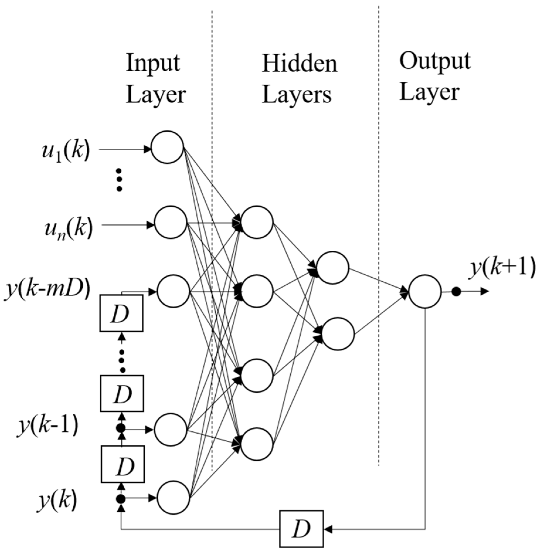
A general discrete model of a NARX is depicted in Figure 2. An analytic description can be given in terms of

$$y\left(k+1\right)=f\left(y\left(k\right), y\left(k-D\right),y\left(k-2D\right),\dots y\left(k-mD\right), u_1\left(k\right), u_2\left(k\right), \dots u_n\left(k\right)\right).$$

(2)

In Equation (4), it becomes visible that only the past values and the momentary value of the n system inputs u and the system outputs y are used to calculate the next value in time domain of the system output y for each time instance k. By delaying past output data and considering them at the system input, the number of past output data and the time interval in which the past output data are considered for calculating the new output data can be varied by m. The discrete time step D reflects the sampling rate $f_{\mathrm{smp}}$ of the entire ANN and consequently quantizes the delay. In this study a sampling rate of 10 kHz and consequently D = 0.0001 s is chosen according to

$$D=\frac{1}{f_{\mathrm{smp}}}.$$

(3)

The NARX represents a feedforward network with an outer feedback loop, in the case of this study for the last current value. After having chosen the general topology, the number of layers and neurons per layer had to be decided. No algorithm to identify an optimal structure of the ANN is known to the authors. Consequently, 22 different NARX networks were studied. The layers, the number of layers, the number of neurons and their activation functions and also the form of the arrangement were varied, e.g., an increasing, a constant and a decreasing number of neurons per layer.

4.2. Training

The ANNs in this study are trained by supervised learning in time domain. Two main aspects specify the training: the optimization algorithm and the set of data that is used.

4.2.1. Optimization Algorithm

For feedforward ANNs, backpropagation through time (BPTT) is a standard optimization algorithm. However, BPTT leads, in the case of recurrent networks to the constraint that a deeper network structure results in a smaller change of the weight. Other algorithms have been developed, such as Momentum and RMSprop that are proposed in Keras [26], a deep learning library in Python. For the optimization of the network, this study applied multiple optimization algorithms. The Momentum algorithm tries to improve the stochastic gradient descent (SGD) that updates the parameters after each training by adding a term with respect to past updates to the current vector in terms of an accumulated gradient. The Nesterov Accelerated Gradient (NAG) algorithm performs the accumulated gradient of previous updates first and corrects afterwards. Like the RMSprop algorithm, the Adaptive Moment Estimation (Adam) considers the exponentially decaying averages of the past squared gradients $v_t$ but additionally takes the exponentially decaying average of past gradients $m_t$ into account while the Nesterov Accelerated Adaptive Moment Estimation (Nadam) algorithm can be seen as a combination of Adam and NAG. The parameter $\theta$ has to be updated for each time step. It can be calculated analytically for the next time step based on the current parameter ${\theta }_t$, the learning rate $\eta ,$ the smoothing term $ϵ$ to avoid zero division, the current gradient $g_t$, the bias-corrected estimate of the current momentum vector ${\widehat{m}}_t$, and the parameters ${\beta }_1$ and ${\beta }^t{}_1$ that affect the decay rates. The analytical description of the update rule according to Nadam is formulated in [27] as

$${\theta }_{t+1}={\theta }_t-\frac{\eta }{\sqrt{\widehat{v_t} }+ϵ}\left({\beta }_1{\widehat{m}}_t+\frac{\left(1-{\beta }_1\right)g_t}{1-{\beta }_1^t }\right),$$

(4)

while a more detailed explanation of the different algorithms can be found, e.g., in [28,29,30].

4.2.2. Data Sets

The data for training and for validation have a major impact on the performance of the ANN. To prevent the network from overfitting, e.g., so that the network does not simply remember the output signal, validation data sets are required. These validation data sets are not used for training. The results of the ANNs with the original validation data over the number of epochs are compared. If the results of the ANNs do not improve by increasing the number of epochs, an overfitting is presumed.

5. Application

5.1. Framework

For this study, the measured data were generated at a test stand in the laboratory. A simulation environment was used to train the ANNs while the results from the ANNs and the measured data are compared afterwards.

5.1.1. Simulation Environment

The study with regard to simulating the device behavior with ANNs, i.e., the training and the validation, was performed in Python with TensorFlow and the library Keras. This allows advanced settings with regard to including own classes and extending basic algorithms. For the comparison of the results achieved by the ANNs and the measurements the software MATLAB was used.

5.1.2. Test Stand

The training and validation data for this study were generated in the laboratory in terms of measurements. The measurements were performed on a commercially available single-phase PV inverter for low-power rooftop applications in LV networks. No knowledge about the inner structure, such as hardware and software components is available. The recorded data contain the DC-side current i_DC and the DC-side voltage u_DC as well as the grid-side current i_AC and the grid-side voltage u_AC at the inverter terminals. A measurement uncertainty better than 10% for currents above 15 mA and voltages above 1 mV is ensured. The voltages are generated by a programmable grid-simulator that can apply the desired voltage waveform at the inverter terminals and supply up to 45 kVA. A PV simulator as a constant power source with a programmable voltage-power characteristic was used to emulate the PV panels for the inverter. The DC-power level is set to 50 % of the rated power of the PV inverter, i.e., 2.3 kW.

5.2. Data Set

Since the ANN is meant to be used also for simulations of transitions between two steady states, the fingerprint as explained in Section 3.3 has to be extended. Instead of only measuring one steady state at a time, two steady states including the transition between them were recorded for this study within one measurement. For this study, the transition between two steady states intentionally starts always at the zero crossing in the voltage, where the “lowest” transient response is expected. If the application of ANNs fails even for the most simple transition, the application of ANNs to reflect the time domain behavior of PV inverters is not feasible at all. If the suitability of the ANN can be validated for this case, further studies have to investigate the variation of the start of the transition and the accurate reflection of the respective transients. A general applicability of an ANN for all possible use cases, e.g., time domain stability simulations, large-scale studies of interactions, studies of system transients, etc. requires a much larger amount of data while this article is meant to present an initial study on the feasibility of ANNs for time domain simulations in principle.

The data sets for training are based on single-frequent voltage distortions, i.e., 40 training data sets, according to the principle of the frequency sweep as explained in Section 3.3. An amplitude of $2\sqrt{2} \mathrm{V}$ and a frequency sweep in 50 Hz steps up to 2 kHz is applied. The phase angles and the amplitudes of the excited distorted voltage components were not changed according to the assumption that the current response of the inverter is linear regarding the phase angles and amplitudes in the voltage distortion components.

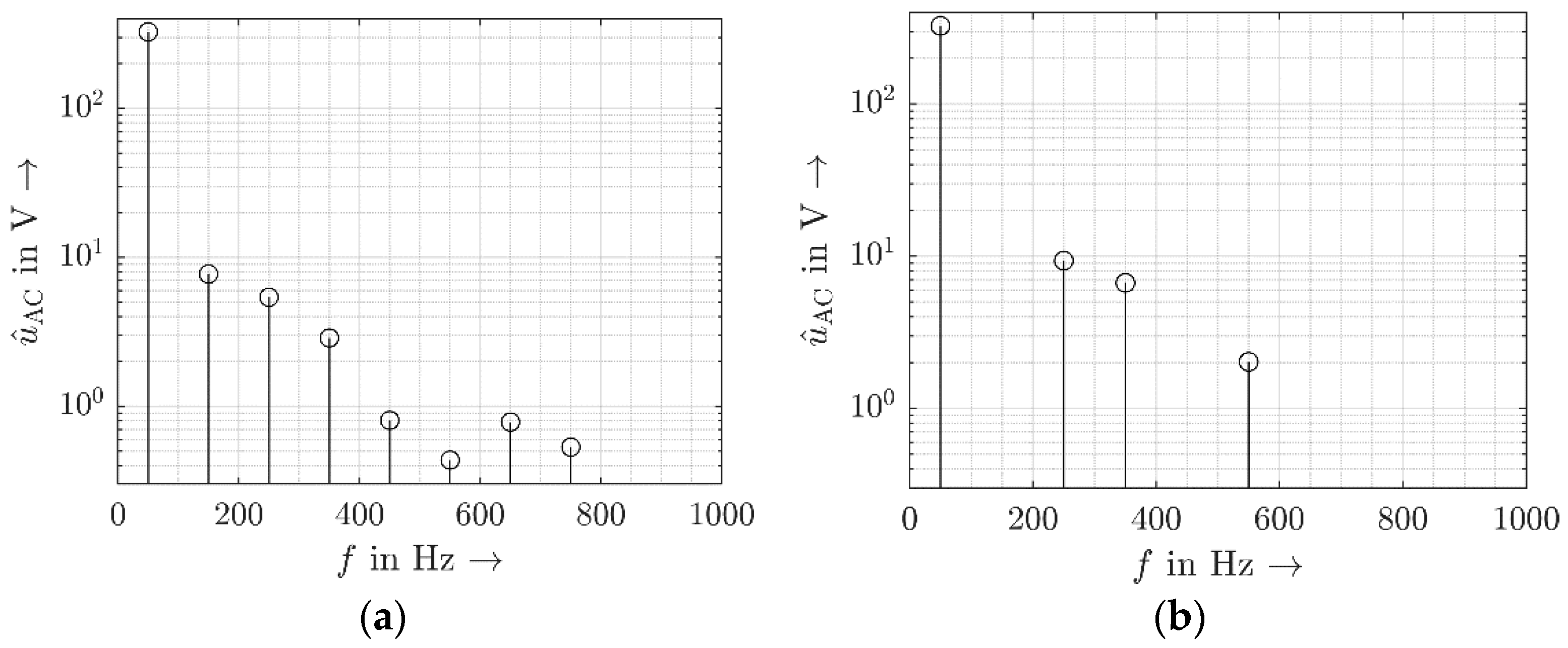
Four validation data sets with different multi-frequent voltage distortions on the grid-side of the PV inverter are applied. Different amplitudes and phase angles were chosen for the distortion components, which represent a considerable deviation from the single-frequent data used for training purposes. The chosen amplitudes considered typical voltage distortion levels in LV networks, e.g., a noticeable presence of 3rd, 5th, 7th and/or 9th order harmonics [31]. This voltage distortion complies with the standards, e.g., the EN 50160. Figure 3 shows the amplitude spectra ${\widehat{u}}_{\mathrm{AC}}$ of the four validation data sets.

The original data were measured at a sampling rate of 1 MHz. For the training and validation, the measured data are sampled down to 10 kHz. This is suitable, since the frequency parts above 10 kHz were found to be negligible, so that aliasing does not occur. In case future measurements show a considerable presence of frequency components above the studied frequency rage, appropriate filter techniques have to be applied. According to the Nyquist–Shannon theorem, a representation of the real system by the ANN up to a maximum of 5 kHz is theoretically possible. The down sampling reduces the effort for training as the range of interest is narrowed down to 2 kHz in this study. Each measurement has a length of 2 s. After sampling down to a sampling rate of 10 kHz, each measuring point still includes 20,000 samples. An improvement of the training can be achieved if these 20,000 samples are restructured into so-called batches with a size of 1000 samples.

5.3. Comparison of NARX Structures

The output layer of the ANN always consists of a single neuron representing the AC-side current of the time step k+1. The input layer contains a different number of neurons related to the DC-side current, DC-side voltage, AC-side current and AC-side voltage. The number depends on the “memory”, i.e., the number of time steps m into the past and can be different for the different parameters. The number of hidden layers is varied between three and six, while the number of neurons per layer is varied between 40 and 400. Furthermore, the number of neurons per hidden layer was kept similar, decreasing from input to output and decreasing from input to output. Different activation functions, like linear, sigmoid and hyperbolic tangent were studied for the input layer, the output layer and the hidden layers.

The best results were achieved when the number of neurons decreased from the input to the output layer. For the input and output layer, a hyperbolic tangent activation function was identified as most suitable, while for the hidden layers a simple linear activation function is most promising. For the input layer a total of 281 neurons with one value for the DC-current, the last 40 values of the DC-voltage and the last 120 values of the grid-side voltage and the last 120 values of the grid-side current, i.e., m is set to 120, gave the best results. The most suitable number of hidden layers is two with 250 neurons in the first and 50 neurons in the second hidden layer. The overall structure of the NARX network is therefore 281-250-50-1.

5.4. Comparison of Optimization Algorithms

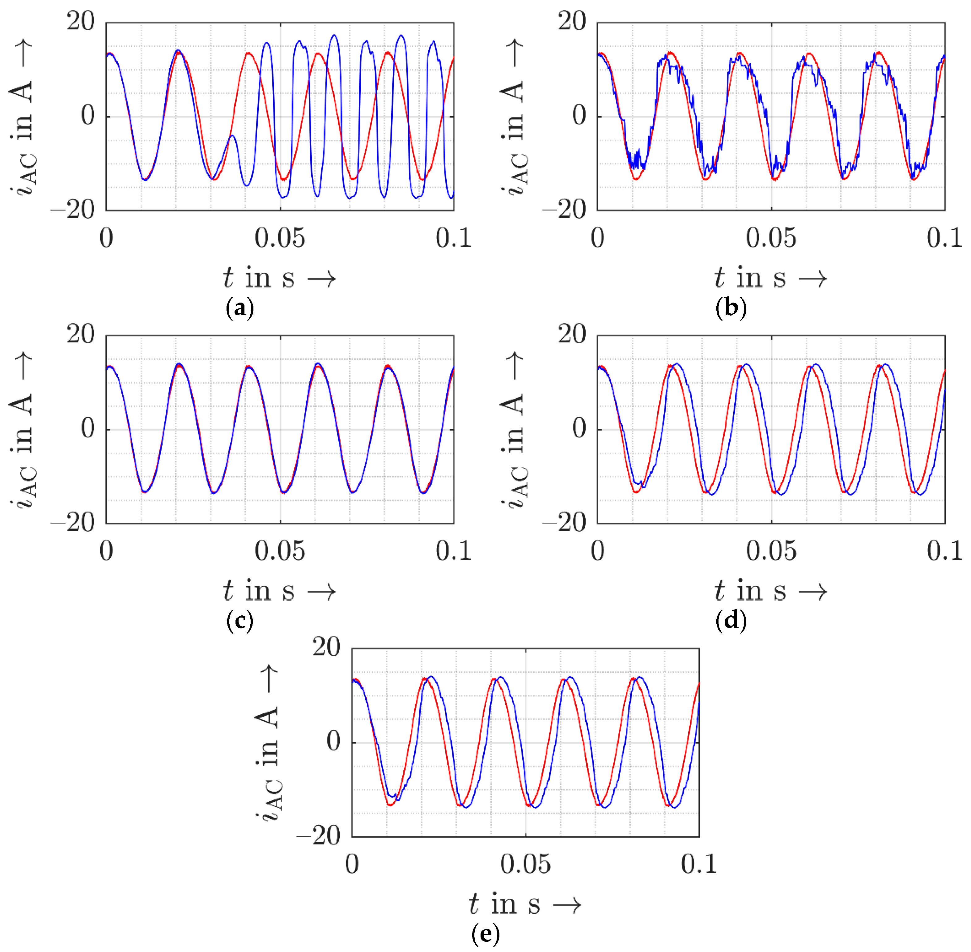
The optimization algorithms introduced in Section 4.2.1 were compared for the most suitable NARX network according to the previous section and a training of 25 epochs. The time domain results are depicted in Figure 4. At this stage, the Momentum and the RMSprop were excluded from the further studies due to their worse performance. A phase shift for the training with Adam and Nadam can be observed, while the results of both algorithms are similar. However, by continuing the training in terms of more epochs, this phase shift diminished and finally disappeared.

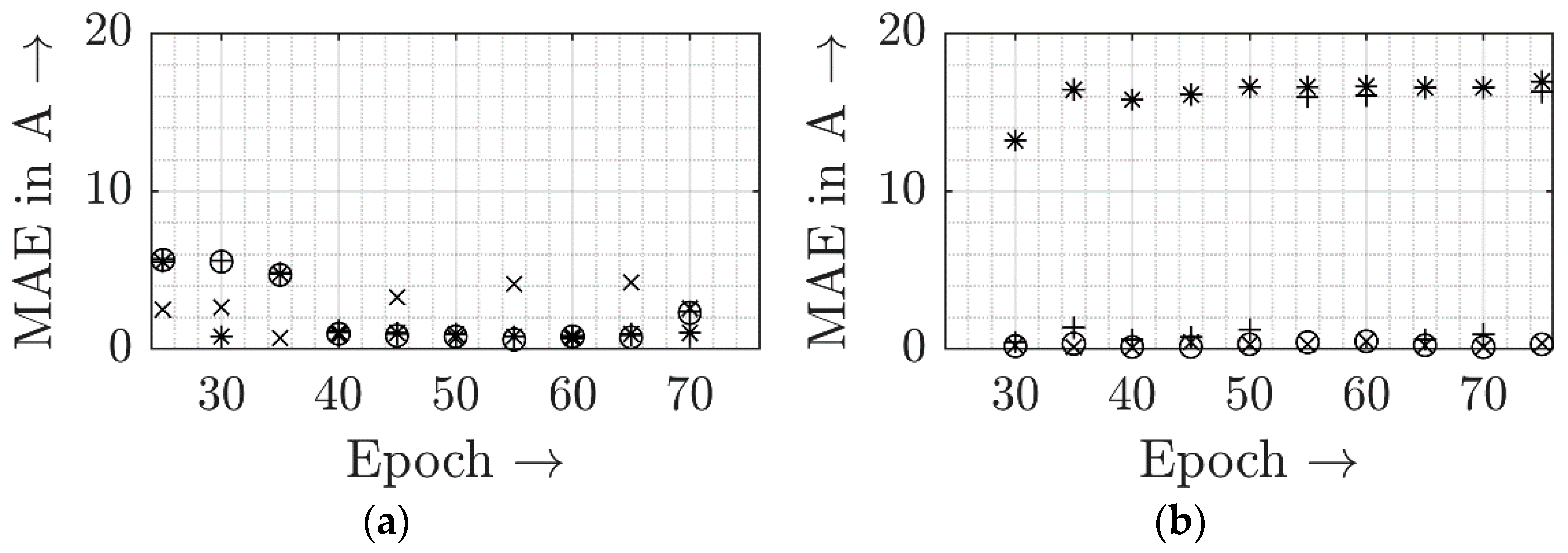
Consequently, only Nadam and NAG were further considered. To evaluate and distinguish the results in time domain between the two remaining optimization algorithms, the mean absolute error (MAE) was calculated for different epochs according to

$$\mathrm{MAE}=\frac{{{\displaystyle \sum }}_{r=1}^R\left(i_{\mathrm{ANN} r}-i_{0 r}\right)}{R}$$

(5)

where $i_{\mathrm{ANN}}$ is the predicted value, $i_0$ is the observed value and each r represents a real value data point of all data points R. While in this study only the MAE was analyzed, further factors can be evaluated, e.g., as proposed in [32]. All validation measurements were considered for the evaluation. The results of the improvement over the epochs with respect to the optimization algorithms Nadam and NAG are presented in Figure 5. The optimization with the NAG algorithm was worse than with Nadam. The best results are achieved with Nadam after 50 epochs.

5.5. Detailed Results

Two main aspects were the focus of this study: the feasibility of ANNs to reflect the accurate steady state behavior, i.e., the frequency couplings, in a time domain model and second, the feasibility of ANNs to predict the transition from one steady state into another. The following sections present the results for the most suitable ANN (NARX network with layer structure of 181-250-50-1, Nadam optimization algorithm and 50 epochs of training).

5.5.1. Steady State Results

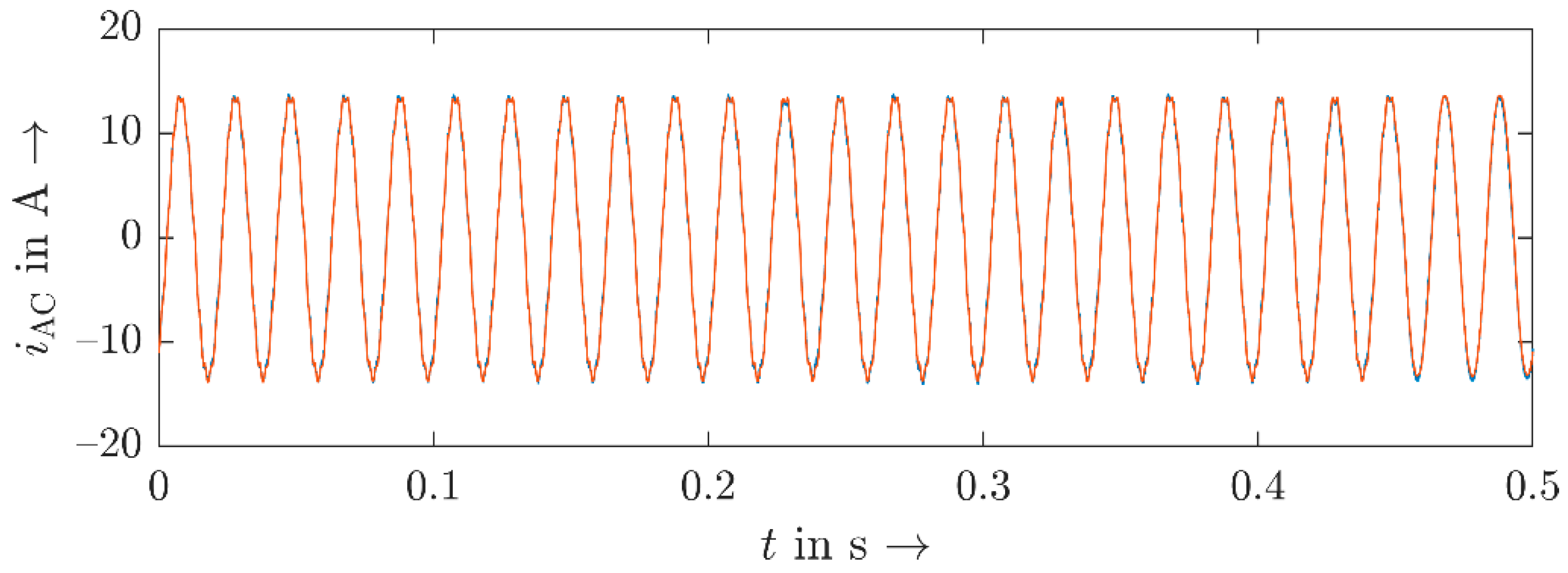
Before analyzing the accuracy, the stability of the results for longer simulation times is assessed. Figure 6 shows that the NARX can provide a good representation of the grid-side current also for a considerably longer time, e.g., 0.5 s. The predicted current and the real measured current do not drift apart so that they appear similar.

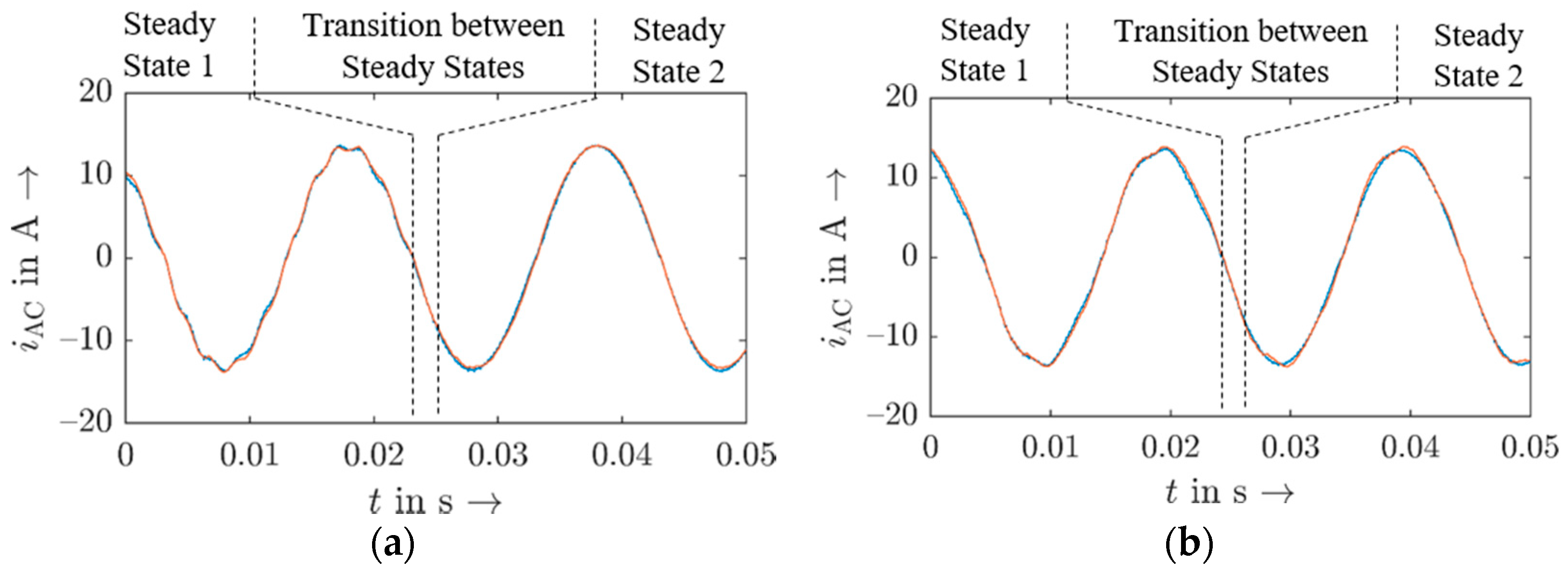
The results for the steady state prediction are exemplarily shown for a single-frequent supply voltage according to the training results and a multi-frequent supply voltage distortion with regard to the validation data in Figure 7.

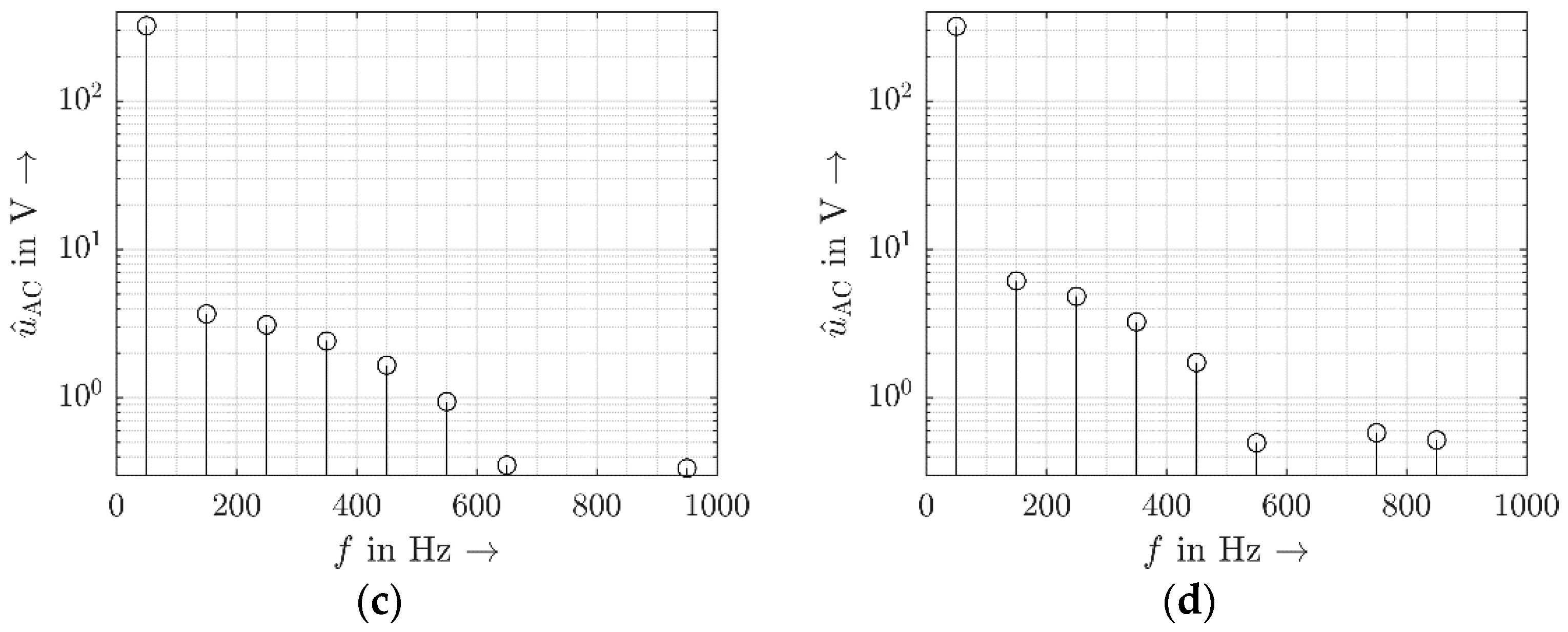
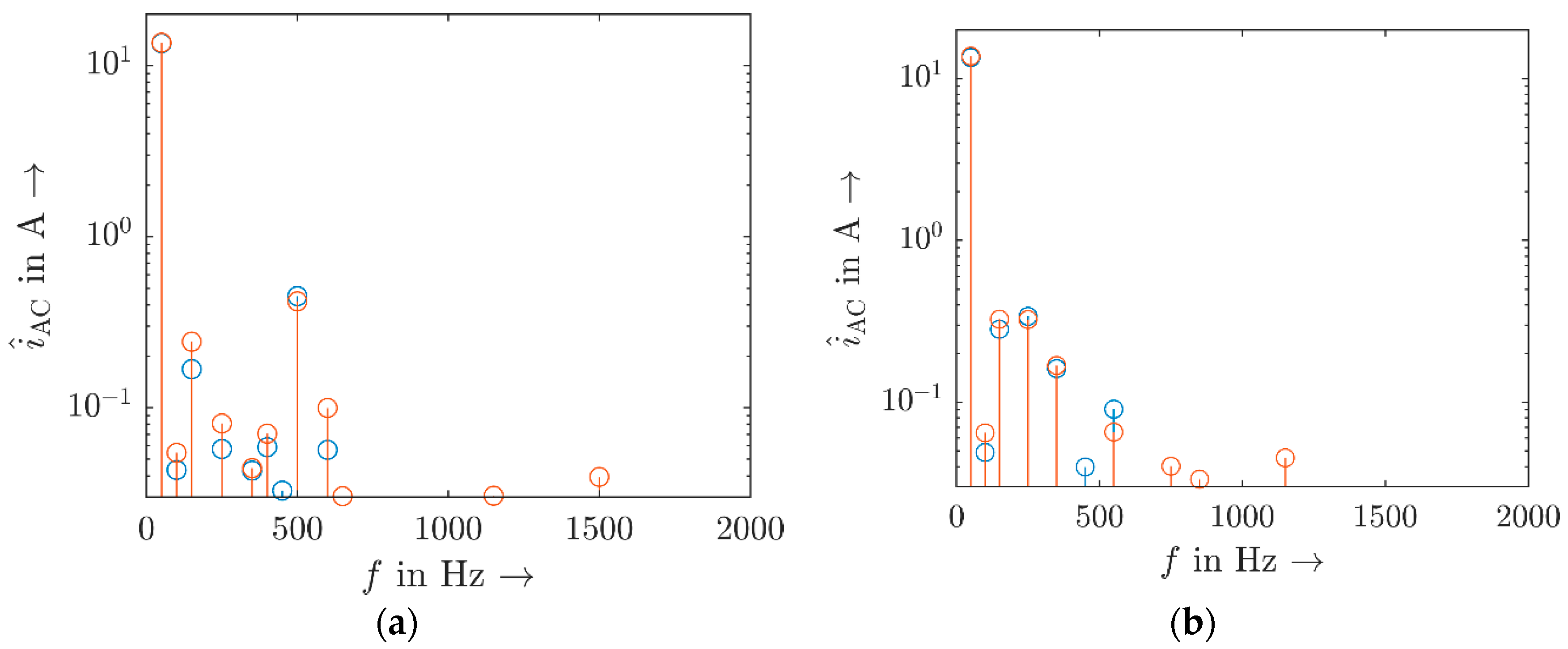
The single-frequent distortion consists of a 10th order harmonic distortion (500 Hz) added to the fundamental component of the supply voltage at the grid-side inverter terminals. While the applied voltage distortion consists only of one frequency component, the spectrum of the measured grid-side current response in Figure 8a shows additional frequency components (frequency couplings) next to the fundamental and the 500 Hz component. These components, typically multiples n of twice of the fundamental frequency f₁, so with 2nf₁, were also represented in the simulation with the NARX.

Figure 8b shows exemplarily that the NARX can also accurately represent the spectrum of the grid-side current for a multi-frequent voltage distortion, i.e., validation data set 1 according to Figure 3a. Additionally, for this case the spectrum of the predicted current waveform matches fairly well with the measured one.

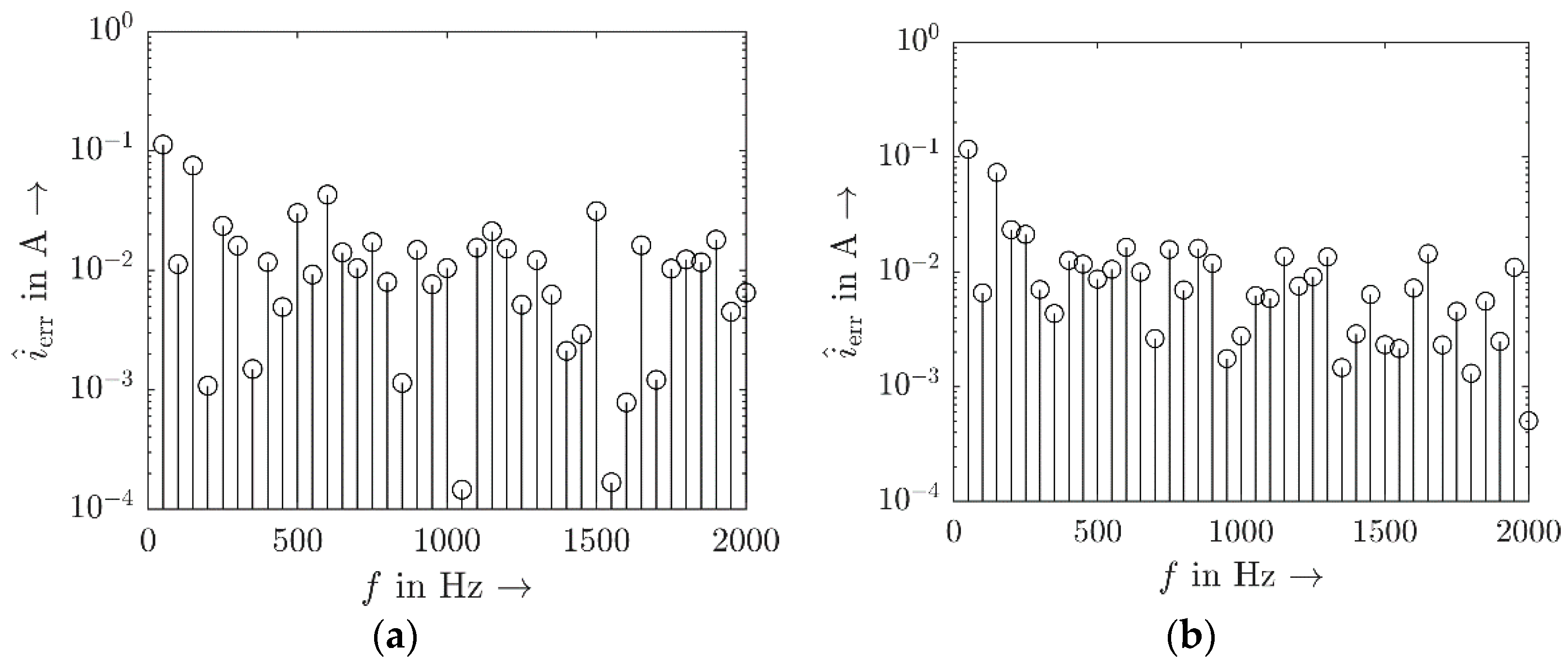
This was tested for all four validation data sets. The simulative results achieved by the NARX show a deviation below 110 mA compared to the measured data (e.g., Figure 9). The absolute deviation ${\widehat{i}}_{\mathrm{err}}$ of the measured amplitude î_{AC meas} and the amplitude î_{AC ANN} predicted by the ANN is calculated in terms of

$${\widehat{i}}_{\mathrm{err}}\left(f\right)=\left|{\widehat{i}}_{\mathrm{AC} \mathrm{meas}}\left(f\right)-{\widehat{i}}_{\mathrm{AC} \mathrm{ANN}}\left(f\right)\right|.$$

(6)

The implementation in time domain results in a rather absolute deviation in frequency domain, i.e., dominant frequency components are represented relatively more accurate than the small frequency component.

Calculating the relative error is not suitable, since already small absolute deviations for very small measured signals, e.g., some mA, imply an enormous relative error while this relative error is not representative.

5.5.2. Transition between Two Steady States

Next to the accuracy of the steady state behavior in time domain, it was studied if the ANNs can simulate a change between two steady states and converge into the new steady state.

In Figure 7a the transition from a single-frequent distorted operating point, the previously shown 500 Hz distortion, to an operating point under non-distorted, i.e., sinusoidal, conditions is shown. The ANN is able to perform the transition into the new steady state by providing appropriate results before, during and after the transition.

In Figure 7b, an extract of the multi-frequent current response is shown. At the zero crossing after about 23 ms, the voltage signal is changed from the distorted signal to the purely sinusoidal voltage. The simulated current response matches the measured current response before the transition, i.e., steady state 1, during the transition and after the transition, i.e., steady state 2.

6. Discussion

This study is the first of its kind attempting to represent an entire PE device (i.e., a PV inverter) by ANNs as black box model in time domain. It aims to assess the feasibility in principle of such a model approach and its potential for further improvement. Related to this initial research the following general observations can be made.

6.1. Frequency Range

The study was performed by considering the frequency range up to 2 kHz. Dynamic changes are therefore also limited to this frequency range. While the change of the grid-side voltage was applied for this study only at zero crossing, a change at the maximum of the fundamental frequency can trigger a transient current response that contains frequency components far above 2 kHz. Laboratory measurements have shown frequency components between 5 kHz and 55 kHz for different commercially available PV inverters [33].

As the ANNs in this article are trained for frequencies below 2 kHz, transitions between two steady states containing frequency components above 2 kHz are expected not to be properly simulated while, for switching during zero crossing, the natural system does not introduce dominant current components in the frequency range above 2 kHz; this cannot be generalized for switching during other time instances [33,34] and needs to be addressed in future studies. However, the focus of this study is the rather slow changes compared to high frequency transients, since known instabilities caused by control interactions typically occur in the frequency range below 2 kHz. Due to the bandwidth of the controller and therefore the passive behavior of the PV inverters in the frequency above 1 kHz, this transient behavior is not expected to cause instabilities, e.g., according to passivity-based control theory. Consequently, the limitation to 2 kHz seems to be sufficient for studies related to harmonic instabilities.

It can still be of interest to train ANNs in future studies to consider the frequency range above 2 kHz to simulate the transient behavior, e.g., to analyze unwanted tripping caused due to too high a current rise. However, to include higher frequencies, the optimal layer structure has to be identified anew. It is expected that the number of epochs as well as the complexity of the overall ANN structure increases with an increasing frequency range.

6.2. Data Set

For ANNs, it is always a challenge to predict the behavior for scenarios that are not properly covered in the training process. Therefore, the data set for training should cover all relevant operating points with a suitable amount of data for training as well as validation. While for this study, only transitions between a steady state with distorted voltage, i.e., single-frequent or multi-frequent distortion, to a sinusoidal voltage are considered, consequently, the data set for training and validation should be extended to transitions between two steady states containing different voltage distortions as well as real harmonic instabilities.

6.3. Electrical Network Simulation

For this study, the measured voltage at the PoC was fed to the ANNs via the system inputs u. It is the final aim to obtain the resulting voltage at the PoC based on the injected current of the PV inverter by integrating the ANNs into suitable network simulation software, i.e., electromagnetic transients (EMT) software for time domain studies. This can be achieved by either a direct implementation of the ANNs, or, e.g., by a controlled current source to complete the representation of the entire power system including the LV network.

Advantages of using ANNs are smaller simulation durations and the reduced computational effort compared to classical white-box simulations in time domain. While the training demands a time effort of several hours to days, the simulation of the current with a completely trained network takes only several seconds. This depends on the previously introduced discrete time step length defined by D, while it has been found that the solver accuracy also has to be set appropriately for classic electrical network simulations [35]. In an exemplary direct comparison, the ANN was able to reflect 0.5 s of the grid-side current in 30 s while the white-box model in MATLAB/Simulink took about 4 min.

7. Conclusions

7.1. Summary

The study presents a study on the feasibility of ANNs for modeling single-phase commercially available PV inverters in time domain. By using a measurement-based set of training data generated by an adapted frequency sweep and multi-frequent validation data, a consequent black-box approach was followed. No information about the internals of the PV inverter is required. Different ANN topologies and structures as well as algorithms and parameters for the training were studied systematically. Out of the tested ANN topologies, not all topologies were able to reflect the inverter behavior appropriately. Especially simple ANN topologies faced major challenges, but the more complex LSTM was also not able to reproduce the original data with sufficient accuracy with a similar amount of training effort compared to the NARX topology. However, the considered NARX topology demonstrated a suitable solution at a manageable training and implementation effort. The training as well as the validation show good results for the trained operating point so that the NARX ANN proposed in the article provides a feasible topology for black-box time domain models of PV inverters. The steady state behavior of the grid-side current spectrum was accurately reflected for single-frequent and multi-frequent grid-side voltages including the frequency coupling components. Furthermore, the ANN is able to simulate the transition between two steady states for the trained scenario, i.e., during zero crossing. The results of the study show that ANNs are potentially interesting for developing true time domain black box models of modern power electronic devices and further research in this area should be encouraged.

7.2. Future Work

Future work will study the suitability of ANNs to cover more operating points, e.g., different DC-power levels, different changes in grid-side voltage distortion and the interaction between multiple PV inverters. Moreover, the extension of the frequency range by reducing D and subsequently also considering the transients during other points on wave for changing between steady states than zero crossing, e.g., in the maximum of the fundamental that will cause a stronger transient response of the PV inverter, should be analyzed.

Furthermore, though the NARX in the presented structure is able to provide appropriate results, other ANN topologies and structures can be studied and assessed. For the assessment of the training effort, the accuracy of the trained ANNs and the simulation duration, a suitable framework should be developed. Such a framework can provide an overview of the suitability of individual ANNs for different application purposes, e.g., harmonic power flow studies, studies of the transition between two steady states or harmonic instabilities.

Finally, the ANNs have to be integrated into standard network simulation software, e.g., DIgSILENT PowerFactory, to enable large-scale studies of black-box time domain simulations. A future focus of these large-scale studies will be the simulation of LV networks with regard to the behavior of power electronic devices and their interaction, e.g., in terms of harmonic instabilities.