
The Use of a Real-Time Simulator for Analysis of Power Grid Operation States with a Wind Turbine


Faculty of Telecommunications, Computer Science and Electrical Engineering, UTP University of Science and Technology, Kaliskiego 7, PL-85-796 Bydgoszcz, Poland
*
Author to whom correspondence should be addressed.
Energies 2021, 14(8), 2327; https://0-doi-org.brum.beds.ac.uk/10.3390/en14082327
Submission received: 22 February 2021
/
Revised: 24 March 2021
/
Accepted: 13 April 2021
/
Published: 20 April 2021
(This article belongs to the Special Issue Power System Dynamics and Renewable Energy Integration)
Abstract
:The main issue in this paper is the real-time simulator of a part of a power grid with a wind turbine. The simulator is constructed on the basis of a classic PC running under a classic operating system. The proposed solution is expected and desired by users who intend to manage power microgrids as separate (but not autonomous) areas of common national power systems. The main reason for the decreased interest in real-time simulators solutions built on the basis of PC is the simulation instability. The instability of the simulation is due to not keeping with accurate results when using small integration steps and loss of accuracy or loss of stability when using large integration steps. The second obstacle was due to the lack of a method for integrating differential equations, which gives accurate results with a large integration step. This is the scientific problem that is solved in this paper. A new solution is the use of a new method for integrating differential equations based on average voltage in the integration step (AVIS). This paper shows that the applied AVIS method, compared to other methods proposed in the literature (in the context of real-time simulators), allows to maintain simulation stability and accurate results with the use of large integration steps. A new (in the context of the application of the AVIS method) mathematical model of a power transformer is described in detail, taking into account the nonlinearity of the magnetization characteristics. This model, together with the new doubly-fed induction machine model (described in the authors’ previous article), was implemented in PC-based hardware. In this paper, we present the results of research on the operation states of such a developed real-time simulator over a long period (one week). In this way, the effectiveness of the operation of the real-time simulator proposed in the paper was proved.
1. Introduction
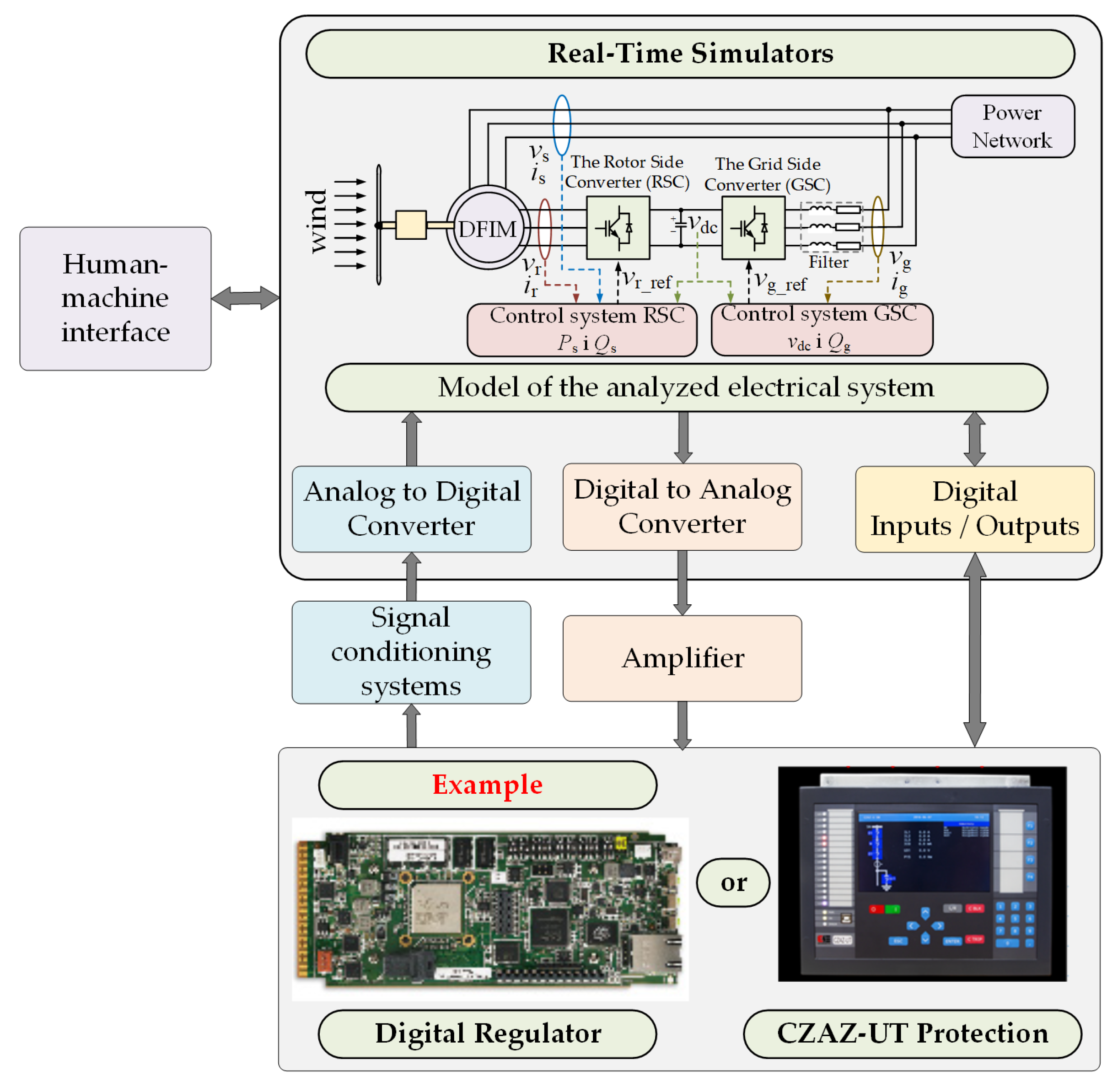
Modern state-of-the-art technology allows for the effective use of real-time simulators in solving many problems related to power systems operations. In the last dozen or so years, many good books [1,2,3,4], doctoral theses (including [5,6,7]) and articles in scientific journals (which will be cited further) have been written about real-time simulators of power systems. This proves that real-time simulators already have an established position in scientific publications, but due to their specificity, not all problems are already solved. This specificity results directly from the valuable advantages of this type of simulators, namely, the possibility of their cooperation with real devices (a regulator with a newly implemented algorithm, a master regulator controlling the entire farm or digital power protection) in real time.
The necessary condition for the correct operation of these simulators is obtaining simulation results at the same time as in their physical counterparts. An example of using a real-time simulator is shown in Figure 1.
A measurable effect of the development of real-time simulators in applications for analyzing the operation of power systems is a number of commercial solutions: RTDS (Real-Time Digital Simulator) [8,9] from the Canadian company RTDS Version 27 September 2020 submitted to Journal Not Specified Technologies and RT-LAB (Real-Time Laboratory) [10,11,12] from OPAL-RT Technologies. The cost of purchasing them is high; therefore, the scientific and research communities are using or looking for cheaper real-time simulators. This group includes simulators based on the DSP (Digital Signal Processor) [7,13,14,15], FPGAs (Field-Programmable Gate Array) [5,16,17,18] and classic personal computers [6,19,20,21,22,23,24].
Statements saying that the time of real-time simulators based on personal computers is over are often made on the basis of works from the end of the last century and are incorrect. Modern personal computers have high computing power and in many practical cases are a competitive solution, combining the technical requirements (of course with limitations as to the extent of the analyzed power system) and the cost of building a complete simulator. That is why such a simulator will be presented in this paper.
A real-time simulator is required to run steadily without interruption or to a scheduled shutdown in order to be able to run concurrently with external processes with an appropriate degree of adequacy, and to run with a constant time step. In order for these requirements to be met, appropriate numerical methods should be sought for the approximation of differential equations and for solving the equation systems of the developed mathematical model. In the above-mentioned publications on real-time simulators (excluding [20,22,24]) and in additional important books on mathematical modeling of power systems [25,26,27], two methods of approximating differential equations are proposed: backward Euler method and trapezoidal rule. The use of the backward Euler method involves a small integration step of the order of single s, so the real-time simulator must have high computing power to be able to obtain the results of the calculations. The trapezoidal method allows one to increase the time step, but there is often a problem of numerical oscillations [5,27,28,29], which may lead to the loss of stability of the simulator operation. This state of knowledge has remained practically unchanged in the last several dozen years. A breakthrough in simulating the operating states of power and electromechanical systems is the use of a new method of approximation of differential equations in mathematical models of these systems, which is systematically developed at the Institute of Electrical Engineering UTP University of Science and Technology in Bydgoszcz (Poland). The real-time simulator described in this article uses this method.
The essence of the method of approximating differential equations in mathematical models of electrical systems is the expansion of the used physical quantities into the Taylor series, but applied to the equations written for average voltages in the integration step. None of the publications listed above (excluding [20,22,24]) mention such a solution. The physical basis of the method was formulated in [30]. In the research conducted at the Institute of Electrical Engineering UTP University of Science and Technology in Bydgoszcz (Poland), this method is successfully used in real-time simulation. Examples of this can be found in [6,20,22,24,31,32,33,34,35,36,37].
The aim of the work, the results of which are presented in this article, was to develop a real-time simulator of the operation of a fragment of the power distribution network with a wind turbine, which will be characterized by stable operation for a relatively long time (at least one week) with appropriate accuracy of the results, taking into account various dynamic processes inside and outside the simulator. This problem was analyzed in detail in the unpublished doctoral dissertation [6]. The applied methods and their effectiveness allow us to state that stable real-time operation of a complex electrical system simulator is possible in a relatively long time, with a relatively long time step, while maintaining the appropriate accuracy of results.
The organization of this article is as follows. In Section 2, we present for the first time the theoretical advantage of using the average voltages in the integration step method in relation to using two other methods proposed in other publications for the RL circuit case. For this purpose, the amplitude and phase characteristics were determined for the system operator transmittances in discrete time H(z) in relation to the solution accurate in continuous time H(s) for three different methods used to analyze the RL circuit. The obtained characteristics were confirmed by example (average voltages in the integration step and trapezoidal rule methods) with practical simulation results that allow for proper interpretation and proof of the advantage of the applied method over two others. Section 3 describes the issues related to the mathematical modeling of a transformer, taking into account the nonlinear magnetization characteristics. The advantage of transient simulation with the use of the average voltages in the integration step method compared to the trapezoidal method was demonstrated. The transformer model was used in the model of a fragment of the power distribution network with a wind turbine, which is described in detail in Section 4. This model was implemented in a real-time simulator constructed by the Institute of Electrical Engineering UTP University of Science and Technology in Bydgoszcz (Poland) on the basis of a personal computer, running under the Windows operating system. The constructed simulator was tested, taking into account dynamic processes caused by events programmed inside the simulator, as well as events taking place in its real environment. The description and results of selected operating states of the simulator are presented in Section 5. The apparatus used, i.e., a real power network parameter analyzer, allowed us to obtain results confirming the stable operation of the simulator in a relatively long time (one week). Section 6 contains drawn conclusions.
2. Accuracy Assessment of the New Method for Approximation of Differential Equations
The accuracy of the applied method for approximation of differential equations is assessed using the method present in many publications [5,27,28,38]. This method consists of comparing the amplitude and phase characteristics of the transmittance ratio H(z) for discrete equations in time to H(s) for continuous equations in time as an exact solution. Additionally, the physical interpretation of the transient analysis is presented for an exemplary electrical circuit, the diagram of which is shown in Figure 2. The analyzed electrical circuit consists of a series connection of resistance R and inductance L, powered from an ideal source of sinusoidal voltage v(t). The circuit parameters adopted in the simulation: resistance R = 0.1 , inductance L = 10 mH, voltage source amplitude Vm = 300 V. The mathematical equation describing the two-terminal circuit is as follows:
Three methods of approximation of the differential Equation (1) will be compared, namely, backward Euler method, trapezoidal method and the method based on average voltages in the integration step (acronym AVIS).Table 1 summarizes the operator transmittance for the electric circuit shown in Figure 2 and the operator transfer functions for these three methods in the application to the same circuit.
The operator transmittances H(z) have been derived for the equation:
which is the transformation of Equation (1) to the discrete form.
The ratio for the considered integration methods is shown in Figure 3 and Figure 4. In these figures, the frequency axis is labeled based on the per unit system, so the Nyquist frequency .
The analysis of the frequency characteristics presented in Figure 3 and Figure 4 shows that the accuracy of the solution using the backward Euler and trapezoidal rule algorithms depends on the value of (voltage frequency or integration step). As the value of increases, the amplitude errors for both methods also increase. The phase error of the backward Euler method also increases with the increasing value of . The phase error of the trapezoidal method is close to zero in the entire range of values under consideration. The conclusion is that the backward Euler method and the trapezoidal method gives fairly accurate answers up to 1/5 of the value of .
Particularly noteworthy is the fact that the AVIS method used in this case is characterized by the amplitude and phase error close to zero, regardless of the value in the entire range of the considered values. This is a convincing proof of the advantage of the AVIS method, compared to the backward Euler and trapezoidal rule method.
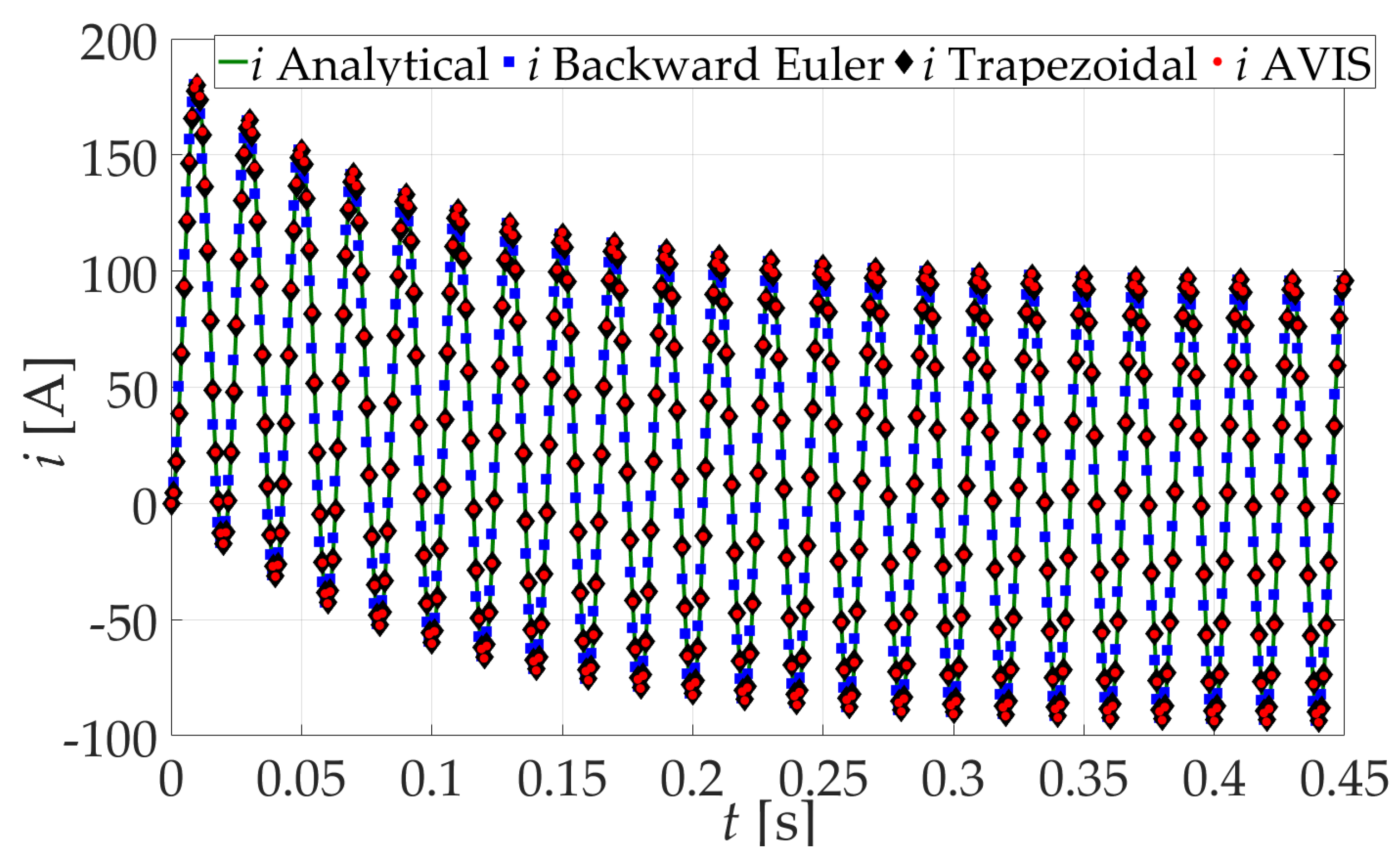
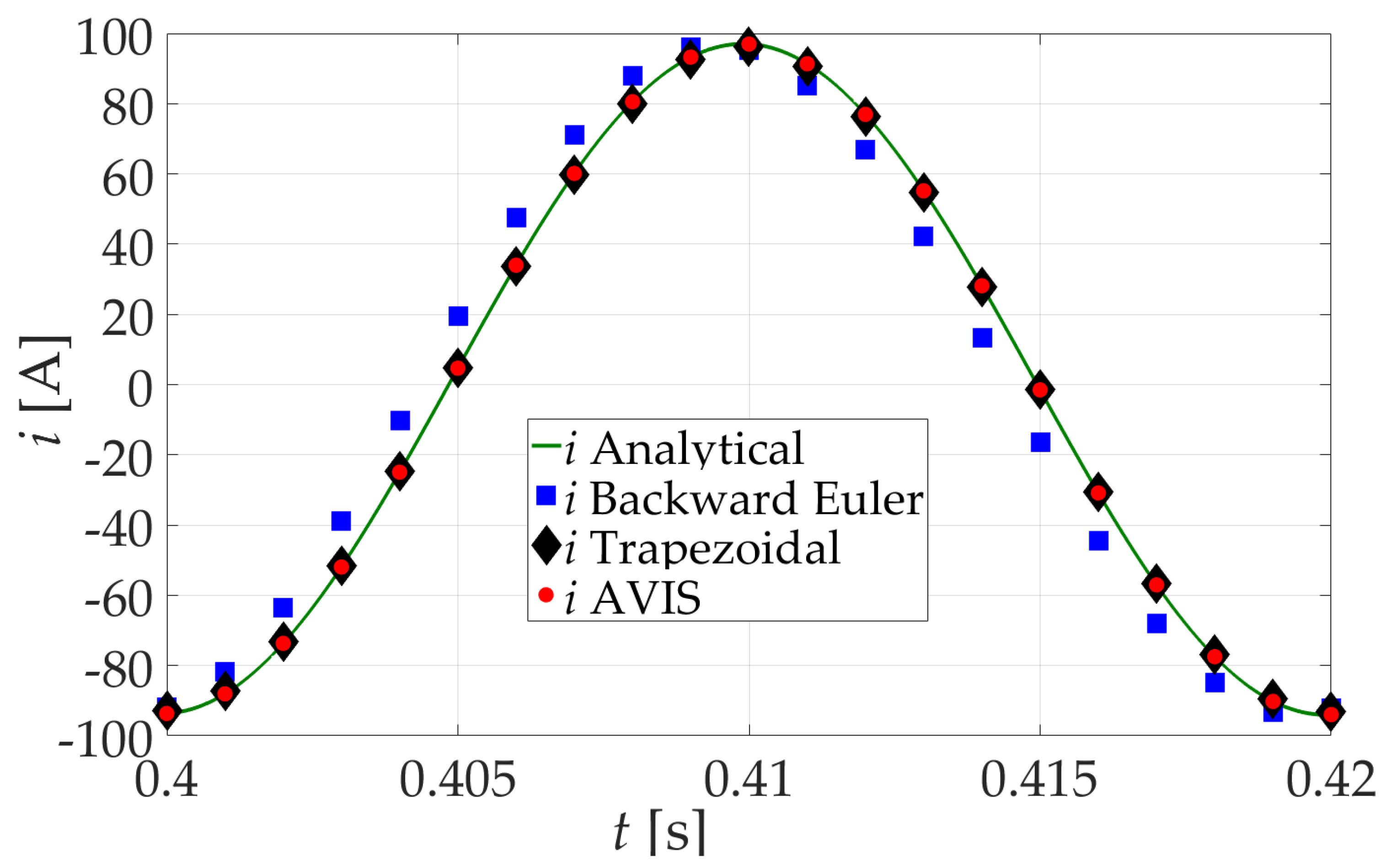
To illustrate the obtained results in practice, a simulation of the transient state caused by connecting the RL terminal block to the AC voltage source was performed. The circuit parameters adopted in the simulation are: resistance R = 0.1 , inductance L = 10 mH, voltage source amplitude Vm = 300 V. Simulations were made with a constant integration step = 1 ms for two values of the supply voltage frequency: 50 Hz and 150 Hz. Figure 5 shows the course of the current flowing in the circuit (Figure 2) after connecting the RL duplex to a voltage source with a frequency of 50 Hz. The current waveforms obtained using the three discussed methods of integration and the current waveform with the exact solution are shown. Additionally, Figure 6 shows a fragment (details can be seen) of this course in the time interval from 0.40 s to 0.42 s.
Figure 7 shows the course of the current flowing in the circuit after connecting the RL double socket to a voltage source with a frequency of 150 Hz. Additionally, Figure 8 shows a fragment of this course for the time from 0.40 s to 0.41 s.
When analyzing the results of simulation experiments, it can be seen that for the integration step = 1 ms, regardless of the frequency of the supply voltage, the most accurate results are obtained using the AVIS method for the approximation of differential equations. Discrete values of solutions coincide with the exact solution. This also confirms the correctness of the results presented in Figure 3 and Figure 4. With the use of the trapezoidal method for a voltage excitation with a frequency of 50 Hz, the results are also satisfactory, but for a frequency of 150 Hz, there is clearly a difference in relation to the exact solution (there is an amplitude error). The use of the backward Euler method in both cases (50 Hz and 150 Hz) causes clear differences in relation to the exact solution.
The analysis also shows that in the analyzed case, with the use of the backward Euler method, in order for the simulation results to be acceptable in terms of accuracy (the amplitude and phase error is small compared to the exact value), the integration step should be reduced ten times compared to the AVIS method. However, in the case of using the trapezoidal method, the integration step should be reduced twice as compared to the AVIS method. Reducing the integration step causes an increase in the time needed to simulate the transient states in the presented dipole. Increasing the computation time in order to obtain greater accuracy of results is not the right solution in the context of real-time simulators.
The results presented in this section clearly prove the advantage of the AVIS method used over the backward Euler and trapezoidal rule method, used by other authors in real-time simulation, for the simulation of an exemplary electric circuit.
3. Simulation of the Operating States of a Power Transformer
One of the elements frequently present in power grids is a transformer. The representation of the dynamics of transformer operation, mainly due to the nonlinearity of the magnetization characteristics and the core remagnetization process itself, is not a trivial issue, especially in the context of real-time simulation. This section presents the results of the test of the accuracy of simulation of transient states of the power transformer operation. Transient states during the transformer connection to the power grid and changes in the secondary side load of the transformer were analyzed.
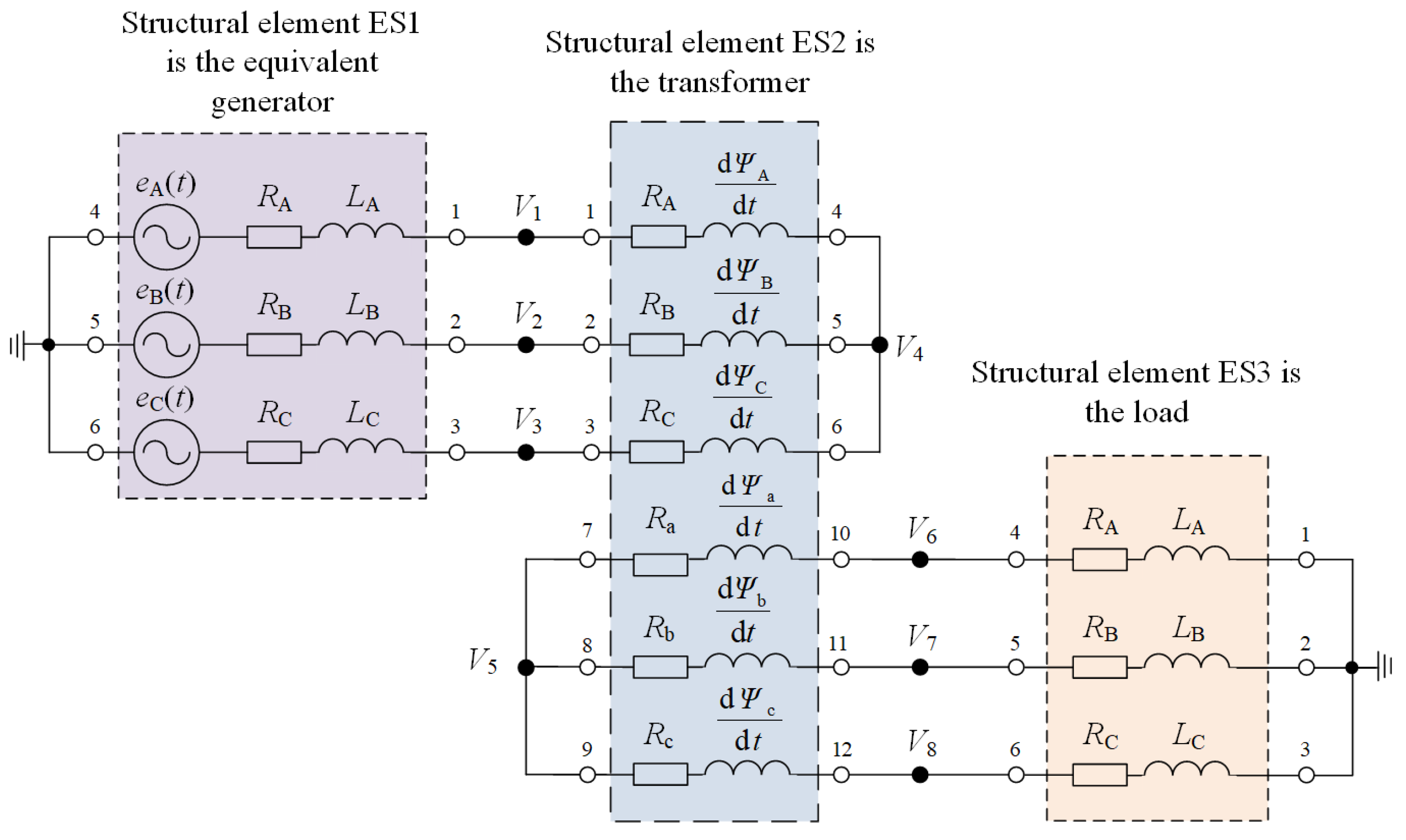
When developing a mathematical model of a power transformer that would allow the simulation of various operating states, the electric multipoles method was used as a method of modeling complex electrical systems. An equivalent diagram of the power system, the test results of which are described in this section, with the division into structural elements is presented in Figure 9. The rated data is given in Table 2.
A detailed mathematical model of a power transformer, developed by the authors of this article, is presented in [24]. When selecting the method of approximation of differential equations, it was taken into account that the developed model can be implemented in a simulator operating in real time. Therefore, the results obtained from such a simulation must be burdened with a small error at a relatively large integration step. It was assumed that the simulation would be performed with an integration step of 50 s.
The performed analysis of the accuracy of the obtained results from the simulation of transient states in the series junction RL (the previous section of this article) made it possible to find out that the results using the backward Euler method do not guarantee the appropriate accuracy. Only two methods were selected for the approximation of differential equations: the trapezoidal method and the method based on the average voltage in the integration step (AVIS). The iterative Gauss–Seidel method was used to solve systems of linear equations. Iterative methods (e.g., the Jacobi or Gauss–Seidel method) allow us to shorten the computation time compared to noniterative methods (e.g., LU decomposition or Gauss’s method) [15].
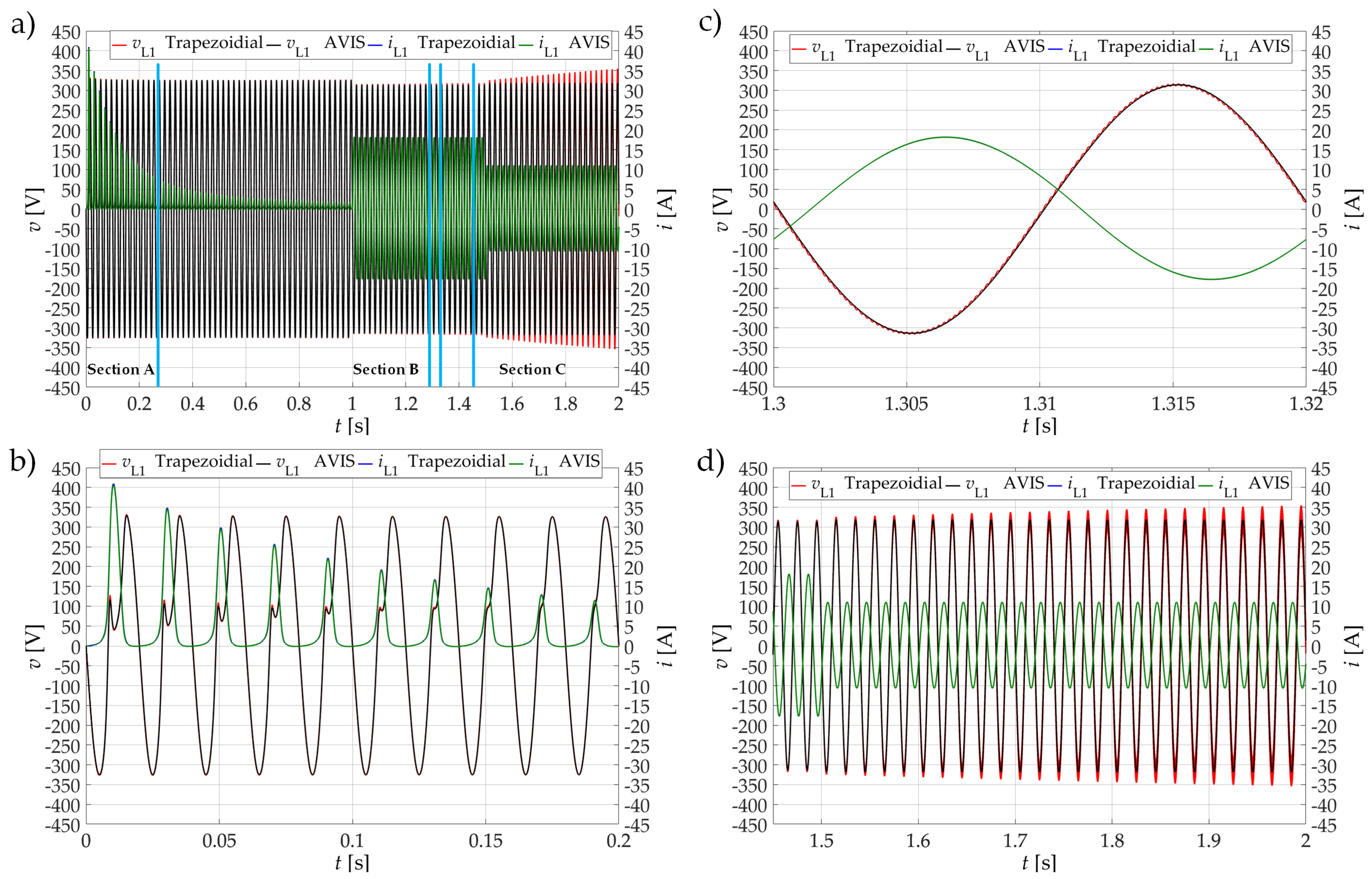
The comparison of the results obtained from the computer simulation with the integration step of 50 s is shown in Figure 10. The trapezoidal method was used to approximate the differential equations in the first simulation, while the AVIS method was used in the second one. The waveforms of the voltage in the L1 phase and the phase current in the L1 phase winding of the power transformer are presented. The following transformer operation states are presented: transformer switching on to the network, time from 0 s to 1.0 s, increasing the load, time from 1.0 s to 1.5 s and reducing the secondary side load of the transformer, time from 1.5 s to 2.0 s.
The presented simulation results with 50 s step confirm that when both of the above-mentioned methods are used to approximate the differential equations, we obtain the same results (Figure 10b,c) for the two considered operating states: switching on and increasing the transformer load. The process caused by the reduction of the load on the secondary side of the transformer, when using the trapezoidal method, causes the simulation to lose stability (the initiation of this process is shown in Figure 10a,d). One of the main requirements for real-time simulators is stable operation over a relatively long time (several days) with various switching processes. Therefore, in the described simulation conditions, the trapezoidal method cannot be used. An effective solution in this case was the use of the AVIS method. The effect of using this method is visible in Figure 10a,d, where after reducing the load on the secondary side of the transformer, the simulation process is still stable. Obviously, the presented results for such a short time do not provide grounds for a general conclusion about the stability of the simulation in a relatively long time (several days). Therefore, the further part of this article presents the results of real-time simulation in the long term for the power grid, including transformer. Of course, the new AVIS method was used in these experiments.
4. Real-Time Simulator of a MV Power Line with a Wind Farm
4.1. Description of the Analyzed Case
The digital simulator is to map the operating states of the medium voltage power line, which supplies the technological park with two main power connections. A Vestas V90 wind turbine (WT) with a rated power of 1.8 MW is also connected to this line. Only this fragment of the MV power distribution network was considered, because its operation is managed by the technology park. The diagram of the analyzed medium voltage distribution line with a wind farm is shown in Figure 11.
Due to the experience in constructing real-time simulators at the Institute of Electrical Engineering UTP University of Science and Technology in Bydgoszcz (Poland), a simulator based on a personal computer was proposed. The simulator has implemented a mathematical model of the power system based on the connection of electric multipoles. A new method based on average voltages in the integration step (AVIS) was used to algebraize differential equations. This problem was the main goal of the doctoral dissertation [6].
In this article, the attention is focused on the experimental demonstration that the developed simulator based on a personal computer working under the MS Windows operating system can work stably with a constant time step for a relatively long time (several days), taking into account the switching and other processes taking place inside the simulator and in its technical environment.
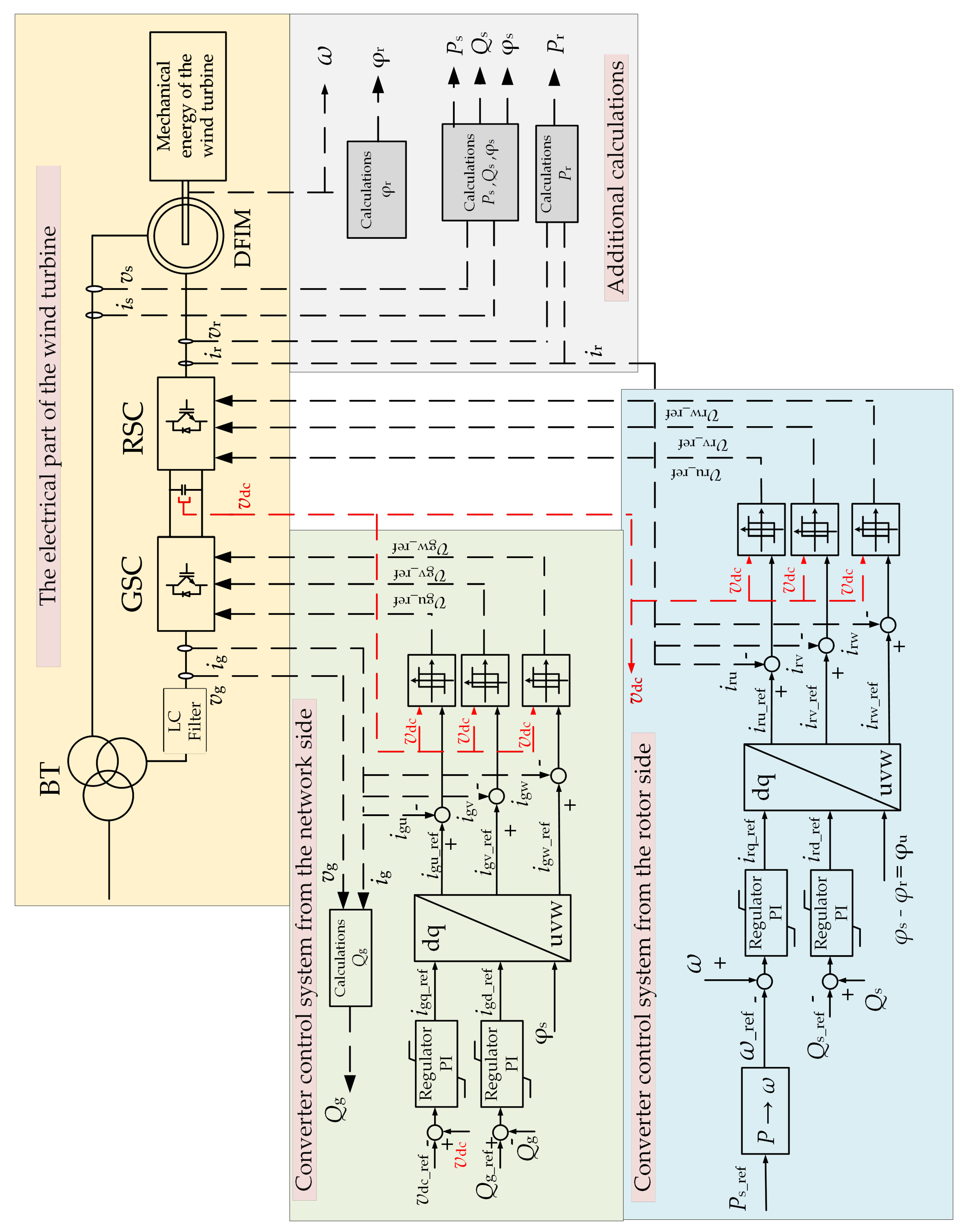
The schematic diagram of the modeled wind turbine with the control system is shown in Figure 12. The electrical part of a wind turbine (WT) consists of the following main elements: a double-fed machine (DFIM); rotor side converter (RSC); mains side converter (GSC); LC filter; three-winding block transformer (TB); the converter control system from the rotor side (RSC) and the converter control system from the network side (GSC). The characteristics of the control system were taken from the literature [9,39].
An equivalent diagram of the analyzed fragment of the MV power distribution network in the form of a connection system of electric multipole poles is shown in Figure 13. In this way, seventeen structural elements were distinguished, the names of which are written directly in Figure 13. This diagram is the basis for the development of a mathematical model of this power system.
4.2. Mathematical Model of the Analyzed Network Fragment
The use of the AVIS method allows for a stable simulation of electrical systems in real time with a relatively large time step (200 s) while maintaining the appropriate accuracy of the results [31,32,33,34,35]. The iterative Gauss–Seidel method was used to solve the system of linear equations.
The basics of mathematical modeling of electrical systems using the above methods are presented in detail in the article [31] by the authors of this article. With regard to the power system considered here, the following structural elements are distinguished: a double-fed induction machine (DFIM), a detailed model of which is presented in [31]; three-winding transformer; power electronic converter, the detailed model of which is presented in [9,39,40] and the MV power line; three loads of electricity (LOAD_1, LOAD_2 and equivalent load) and a replacement energy source (replacement generator), detailed models of which are presented in [31]. Overhead power lines are modeled in the form of multipoles, where each phase of the line is modeled in the form of equivalent circuits with longitudinal (resistance and inductance) and transverse (capacitance) parameters. Electrical loads are also modeled in the form of multipoles where each phase is represented by longitudinal parameters (resistance and inductance).
Due to the fact that the mathematical models of some elements of the analyzed network fragment and the method of creating a mathematical model of the entire system have already been published by the authors of this article (as mentioned above), they will not be discussed here. In this section, only the mathematical model of a three-winding three-phase transformer (BT in Figure 12) will be detailed. Earlier in the work [24], the authors presented a mathematical model of a two-winding three-phase transformer that takes into account the nonlinearity of the core magnetization characteristics.
Using the mathematical modeling convention presented in [31], Figure 14 shows a diagram of a three-winding three-phase transformer as a structural element (eighteen-pole device).
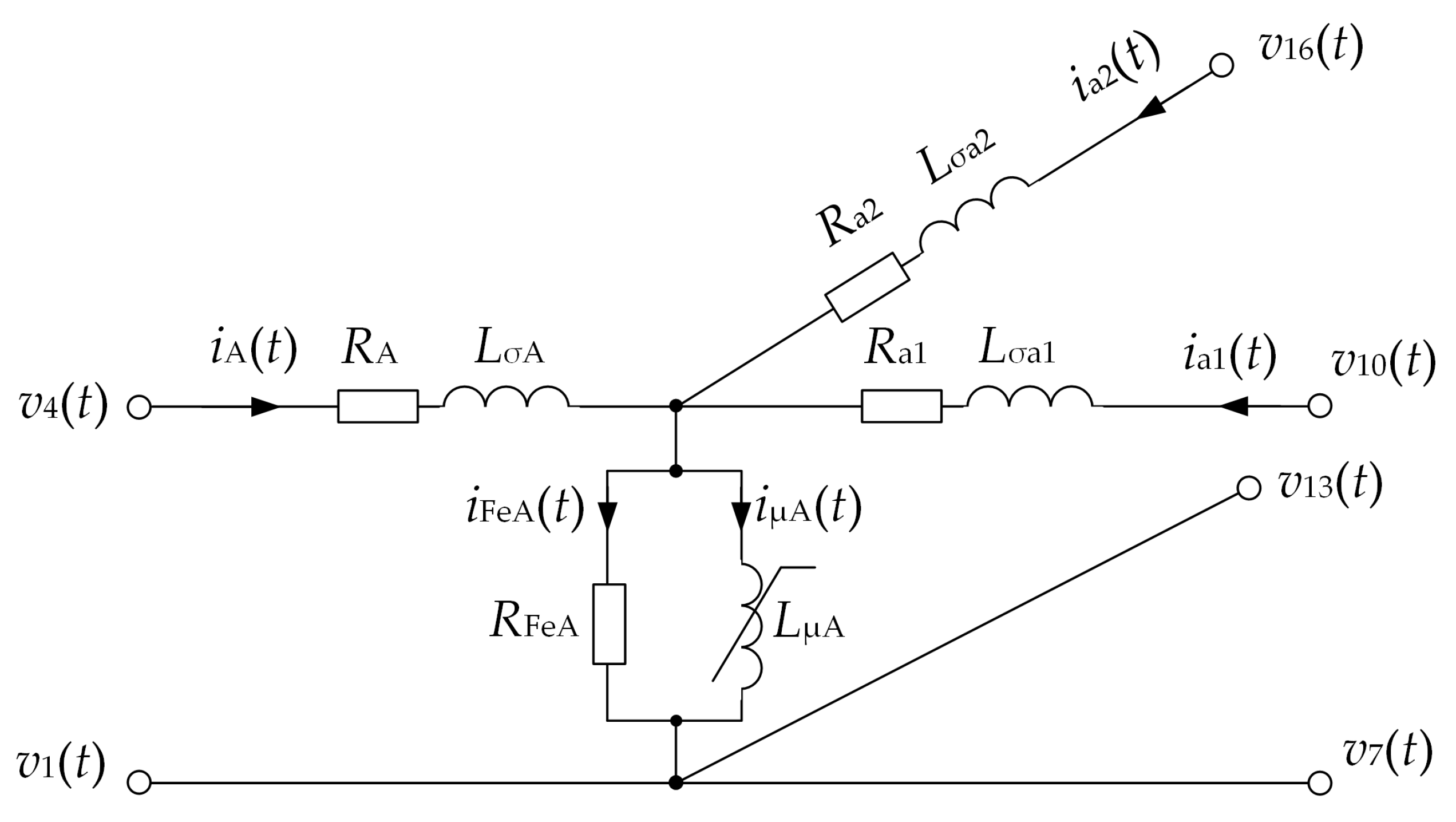
The three-winding, three-phase transformer consists of a three-column ferromagnetic core; on each column, there is placed one upper voltage winding (phase indexes A, B, C) and two lower voltage windings (phase indexes: a1, b1, c1 and a2, b2, c2, respectively). When creating the mathematical model of the transformer, the losses in the core, nonlinear magnetization characteristics and losses in structural elements were all taken into account. A suitable schematic diagram for one phase of the transformer is shown in Figure 15.
The electric circuit of the modeled transformer is described by the following matrix equation:
where:
is a column matrix of the instantaneous values of the main magnetic field fluxes associated with individual transformer windings,
is a diagonal matrix of transformer phase winding resistance,
is a column matrix of instantaneous currents flowing through the windings of individual transformer phases,
is a diagonal matrix of the transformer phase winding dissipation inductance,
is a column matrix of values of instantaneous potentials of winding terminals of individual phases of upper and lower voltages,
n2 it is the transformer ratio of the phase voltage of the upper voltage winding and the phase voltage of the second low voltage winding,
The transformer core is made of a ferromagnetic material, which is characterized by a magnetizing curve, showing the dependence of magnetic induction on the strength of the magnetic field , . This dependence is nonlinear because the relative magnetic permeability of the material from which the transformer core is made is determined by a nonlinear function . Consequently, the relationship between the main magnetic flux associated with the winding of the respective phase and the magnetizing current of this phase is also nonlinear and corresponds to the following magnetizing characteristics:
where: and . These are the coefficients of the approximating function that can be determined by carrying out the idling test.
Taking into account the magnetic characteristics of the main magnetic circuit (4), the matrix Equation (3) can be written as
where:
is a column matrix of instantaneous magnetizing currents for the respective phases,
is a matrix of dynamic magnetic inductance of a ferromagnetic core
To simplify calculations, the matrix of dynamic magnetizing inductances in the Equation (5) has been replaced by a matrix of static inductances, which is determined by the formula:
The introduction of such a simplification enables finding an approximate solution without solving nonlinear equations. After introducing static inductance, the equation describing the electrical circuit of the modeled transformer takes the form of
The full mathematical model of a three-winding, three-phase transformer requires supplementing the matrix Equation (7) with equations describing the magnetic circuit. For this purpose, a surrogate diagram of the magnetic circuit of the modeled transformer was constructed, as shown in Figure 16.
In the magnetic circuit, in addition to the main magnetic field fluxes, an additional magnetic flux is included, representing a part of the magnetic field that causes losses in the transformer structural elements, e.g., tank, cover, beams, flat bars and screws.
Using Kirchhoff’s laws, the following system of matrix equations was created:
where:
is a column matrix of instantaneous currents flowing through the upper voltage windings,
is a column matrix of instantaneous currents flowing through the windings of the first low voltage,
is a column matrix of instantaneous currents flowing through the windings of the second low voltage,
is a column matrix of instantaneous currents causing iron losses,
is a constant reluctance for reproducing losses in transformer structural elements,
it is a magnetic flux that represents the part of the magnetic field that causes losses in structural components,
The current that causes iron losses is determined by the following relationship:
where: , , . These are the resistances reproductions of power losses in the iron of a magnetic transformer circuit.
Integrating the matrix Equation (7) in the range from to , and then dividing by and taking into account the formulas (14), (16), (20) and (21) in [31], this equation takes the following form:
where:
m is the number of terms included in the Taylor series in the mathematical description of branch currents [31],
By making the appropriate mathematical transformations of the above relationships, you can write the formulas for the matrix and , that occur in the key form for the applied method of mathematical modeling of the external matrix equation of the analyzed transformer [31]:
These matrices have the following forms:
and
where:
In order not to solve the system of nonlinear equations, the following algorithm of magnetic field inductance induction prediction was applied in each phase for a moment :
- using the backward Euler method, a matrix of magnetizing currents is determined at the end of the integration step,
- knowing the values of the column matrix of magnetizing currents at the moment determines the magnetic inductance of the magnetic circuit in each phase.
The principle of conservation of energy in a magnetic field results in the principle of magnetic flux continuity, which states that the products of current and inductance at times and should be equal. Determination of the magnetization inductance of the ferromagnetic core in each phase at the moment based on the above method may cause this condition not to be met. Accordingly, based on the work [41,42] in the transformer model, this problem has been approximately solved. The algorithm that takes into account the continuity of the magnetic flux is as follows:
- the matrix of the current flowing through the transformer windings is calculated for the time instant , using the Equation (11),
- for the magnetization inductance determined from the prediction described above, a matrix of estimated magnetizing currents is calculated in each phase using the appropriately transformed upper relationship in the Equation (8),
- the estimated magnetization inductances in each phase are calculated using the formula , where ,
- the modified values of the magnetizing currents are calculated in each transformer phase in a way that ensures meeting the conditions arising from the fact that the products of current and inductance at times and are equal,
- values of corrected magnetizing currents and magnetizing inductance in each phase determined for time are used in the next calculation step.
5. Experimental Studies of Real-Time Simulator Work
5.1. Description of the Experiment
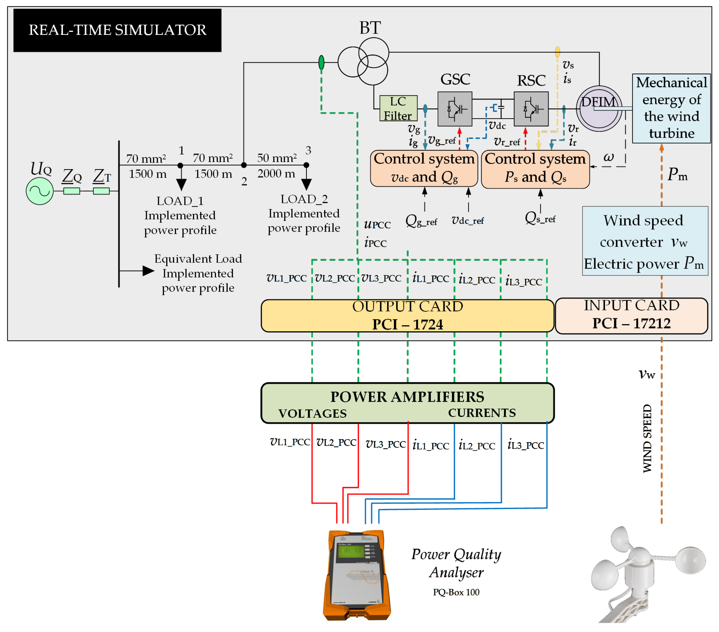
Figure 17 is a schematic diagram of an experimental system that consists of a constructed simulator working in real time with a model of a wind power network, an external real system as an information source, e.g., about the current value of wind speed and a professional analyzer of the network parameters (PQ-Box 100). This section presents selected results of experiments that were the subject of research in the framework of a doctoral dissertation [6].
The simulator working with real time was built on the basis of a personal computer with an Intel six-core processor (Intel® CoreTM i7 970 type) with a clock frequency of 3.20 GHz with a 32-bit Microsoft Windows operating system. The system bus speed is 1600 MHz. The platform has RAM memory (4.00 GB DDR3).
Communication between the environment and the simulator is bidirectional, using digital and analog signals. Advantech PCI-1712 card was used to introduce signals from the environment (e.g., wind speed, power, voltage, current) into the simulator. It is a multifunctional measuring card that allows the use of 16 analogue inputs and 16 digital inputs or outputs. The card is equipped with one analog-to-digital converter working with a resolution of 12 bits and a maximum sampling frequency of 1 MHz or 1 MS/s, which depends on the number of used analog inputs.
Advantech PCI-1724 card was used to output signals from the simulator to the environment (e.g., to terminals on the input signal strip of real controllers, protections). The card allows to activate 32 output channels. Each channel has a digital-to-analog converter working with a resolution of 14 bits in direct mode. This means that the sampling rate depends on the performance of the digital platform used.
The application implementing the simulation process (mathematical model and communication algorithms) was written using the C++ programming language. The application has been written in such a way that provides real-time simulation. When the application is launched, it receives the highest priority, which allows the application faster access to memory or PCI bus (cards with A/D converter or with D/A converters). Giving the application high priority partly solves the problem of proper allocation of resources between individual tasks and protection of allocated resources. Unfortunately, a fully satisfactory solution cannot be achieved using the Microsoft Windows operating system, because the system does not allow full control over the allocation of resources between individual tasks.
The experiment consisted of uninterrupted operation of the simulator during seven days. During that time, the PQ-Box 100 analyzer was connected at the point of common connection (PCC). To create real conditions for connecting the PQ-Box 100 analyzer to the analog outputs of the simulator, voltage and current amplifiers were turned on. The task of the amplifiers is to ensure the electrical compatibility of the simulator output circuits with the external electrical circuits of the real systems. In this case, the amplifiers at the output reproduce the secondary circuits of current and voltage transformers.
In the analysis of the work of the presented power system, the variability of wind speed values and the load variability of three loads identified in the modeled system were taken into account. Current values of wind speed were transmitted from the real external system, whereas the active and reactive power profiles of the loads were set in the form of appropriate schedules, entered into the simulator’s memory.
In addition, random event simulation scenarios were prepared, which are listed in Table 3. These events were initiated in a mathematical model of the simulated system during the experiment. The quantum of the simulator operation time during the experiment was 200 s.
The purpose of experimental research was to verify the work stability of the developed real-time simulator, taking into account the processes caused by the normal operation of system components and including processes initiated by emergency events. The goal was also to check the interaction with the environment and timeliness (verification whether the simulator works with a fixed quantum of operation time).
5.2. Test Results
After the experiment was completed, results were obtained that enable the analysis of the simulator’s work. First, the voltage frequency at the measuring point was analyzed during the experiment. The voltage frequency changes are shown in Figure 18. The average frequency value recorded by the network parameter analyzer is 50.0003 Hz. The recorded voltage frequency values and the average value are proof that the developed simulator is stable throughout the experiment and that the quantum of the simulator’s operation time has been correctly selected. If the quantum of the simulator’s operation time was incorrect (if it was too long, the simulator could not keep up with the calculations), as a result of the simulator’s operation, deviations from the value of 50 Hz would be recorded. A similar result would be obtained in the case of stability of the simulation. If there were any problems with stability, then the voltage frequency deviations from 50 Hz would also be recorded.
The course of effective values of phase-to-phase voltages in PCC is shown in Figure 19. When analyzing the course, it can be observed that changes in voltage values are caused by changing loads of three distinguished loads (active and reactive power profiles), changes resulting from changing wind speed (wind turbine operation) and changes caused by random events. Analyzing in detail the obtained waveforms and events recorded by the analyzer, it is possible to distinguish characteristic operating states, which are marked in Figure 19 by appropriate rectangles (red). The event numbers used in this figure correspond to the numbering used in Table 3.
Figure 20 shows the phase-to-phase voltage variability (L1-L2) at the connection point of the generating unit to the network, registered on 18 October 2018, taking into account the variability of active load power in the analyzed MV distribution network and changes in wind speed. Analyzing these waveforms, three characteristic states can be distinguished. The first of them lasts from to hours. During this period, the load works with relatively low power, while the wind turbine works with the rated power, because the wind speed exceeds 14 m/s. Thus, the voltage variation in the network is caused by changing values of load power, but to a relatively small extent.
The second state lasts from to hours. During this period, the wind speed still exceeds the value of 14 m/s, which means that the wind turbine still works at a rated power. However, at around a.m., there was a clear increase in load power, which causes a decrease in the voltage value, which the analyzer registered. Further analyzing the voltage waveform during this period, it can be seen that at approximately a.m., there was a short-term voltage reduction to approximately 15.75 kV. This is due to the decrease in the supply voltage amplitude in phase L1 planned in the scenario (Table 3) (Event no. 2).
The third characteristic condition lasts from p.m. to midnight. At this time, characteristic fluctuations of the RMS voltage value in PCC can be observed, which are caused by both load variability and wind turbine power variability, due to the fact that at wind speeds below 14 m/s, the turbine power varies according to its characteristics (Vestas V90). The slow voltage fluctuations, which are caused by the change in load power in the network, are superimposed by fast voltage fluctuations caused by the wind turbine.
In further analysis, selected fragments of current waveforms and power generated by the wind turbine for MV distribution network (shown in Figure 21 and Figure 22, respectively) will be considered in detail. From current waveforms, it can be seen that the effective values of currents do not change when the generating unit is working with a constant power value (wind speed higher than the rated speed for Vestas V90 is 14 m/s). In the periods from 16 October 2018 from midnight and 18 October 2018 from a.m., the wind turbine generate electricity with a nominal power of 1.8 MW.
On 17.10.2018, the wind speed exceeded the maximum value for the operation of the wind turbine (v > 25 m/s); therefore, it was turned off. Of course, the value of active power decreased from 1.8 MW to 0 MW (Figure 22), and the effective current value decreased from 66.0 A to 4.0 A (Figure 21). Such changes have a large impact on the voltage value at the node connecting the generating unit to the network (PCC) (Figure 19), as mentioned earlier.
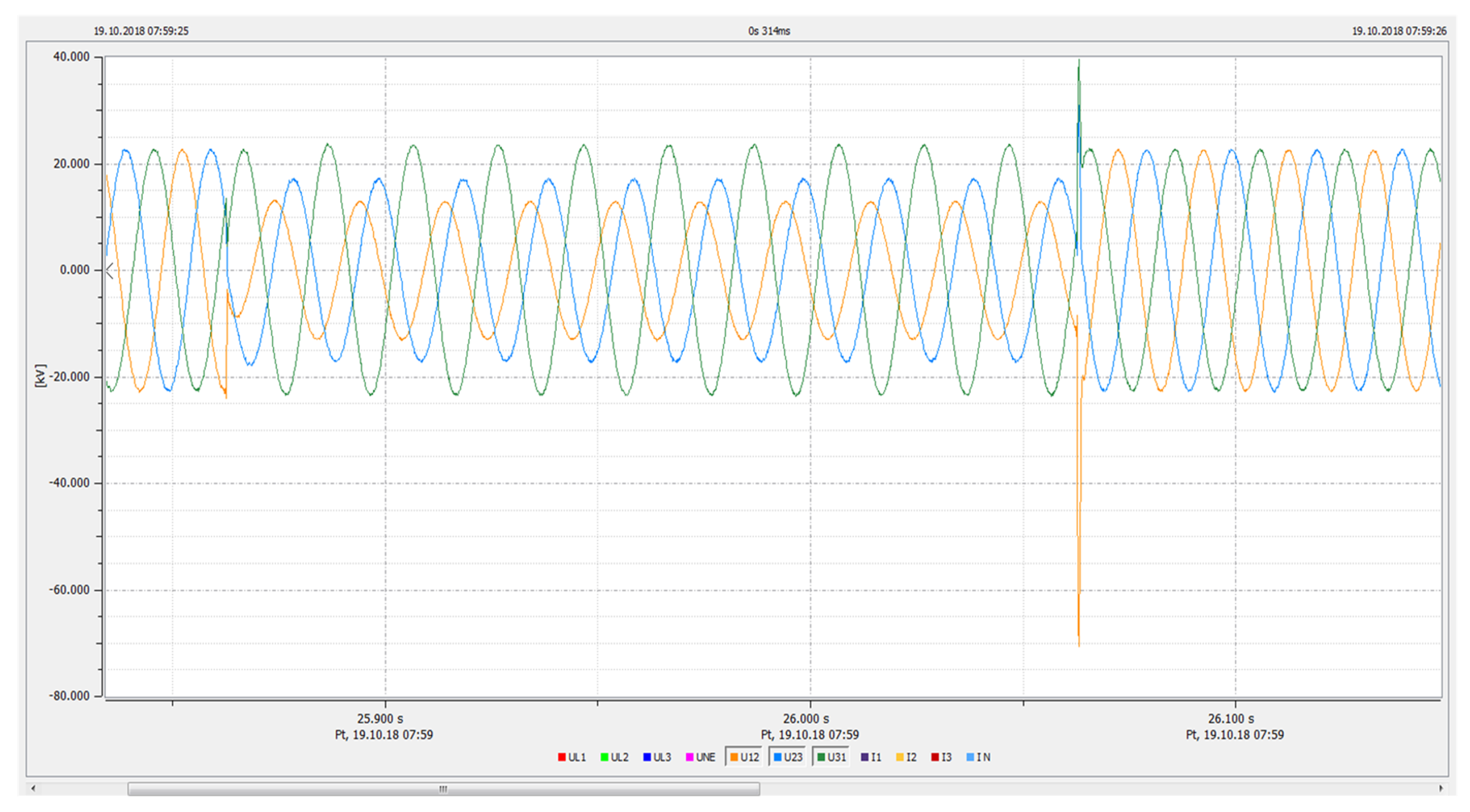
Figure 23 and Figure 24 present waveforms of instantaneous voltages and currents recorded by the PQ-Box during a phase-to-phase short circuit. Figure 23 shows the phase-to-phase voltage waveforms at the generating unit connection node, while Figure 24 shows the waveforms of the block transformer line currents during the phase-to-phase short-circuit (between phases L1 and L2) in acceptance 1 (LOAD_1). The occurrence of a phase-to-phase short circuit in LOAD_1 caused an increase in the wire current in the MV windings of transforme of the generating unit in the L1 and L2 phases. Due to the relatively short fault time, the drawings show the waveforms that characterize the entire process.
Figure 25 shows the time history of phase-to-phase voltages in PCC and the wire currents of the wind turbine transformer on the MV side during normal operation (steady state). The generating unit works with rated power. The phase shift between phase-to-phase voltage and current is approximately 5/6. The asynchronous ring machine works as a generator. Analyzing the course, it can be observed that the quantum of the simulator operation time was correctly selected. This is evidenced by the fact that the frequency of the presented signal is equal to 50 Hz.
Finally, the option of automatically generating a report on the assessment of voltage (electricity) quality at the connection point of the generating unit to the MV distribution network was used, in accordance with the requirements of the PN-EN-50160 standard. This report is presented graphically in Figure 26. The horizontal line corresponds to the limit values for each parameter. Red bars are the parameter values that are not exceeded for 95% of the measurement time; dark blue bars are the maximum value from the set of values averaged during the measurement period. Analyzing the presented results, it can be stated that the quality parameters of electricity in accordance with the standard are met in the node connecting the generating unit to the MV network.
6. Conclusions
The area of broadly understood real-time simulation is currently not fully developed. In the last few years, many good books and publications on this topic have been written. Limiting the applied methods of algebraizing differential equations in real-time simulators to only two (backward Euler and trapezoidal rule), introduced to real-time simulation at the end of the last century, resulted in a tendency to reduce the integration step in order to maintain an appropriate level of accuracy of simulation results. This was considered the only right path in the development of real-time simulation, arguing that a standard personal computer is no longer sufficient for these applications. Work was developed towards the application of DSP, programmable logic circuits and graphics processors. In this regard, many researchers have obtained great results.
However, one should pay attention to the fact that in the future, the power industry will focus on managing local parts of the power systems [43]. From this, the following conclusions should be drawn:
- the demand for real-time simulators will increase, covering areas limited only to a part of the power system, i.e., MV power distribution networks or even only to single (or several) power lines,
- competitive solutions will be sought in terms of costs, both investment and operating costs,
- solutions that are uncomplicated in terms of installation and operation will be sought.
This leads to the conclusion that real-time simulators based on personal computers are going to be of great interest. This article and other work carried out at the Institute of Electrical Engineering UTP University of Science and Technology in Bydgoszcz (Poland) that are intended to meet the future expectations of conscious electricity users.
This article shows that:
- the use of the new AVIS method of algebraizing differential equations, which is based on average voltages in the integration step, allows real-time simulation with a large integration step of 0.2 ms in period of one week while maintaining appropriate accuracy of results,
- the comparison of frequency responses in the RL system with three methods (the known backward Euler and trapezoidal methods and the new AVIS method) in a wide frequency range up to the Nyquist frequency per unit showed that the AVIS method practically does not introduce magnitude or phase error, which is an advantage of this method over two others that are recommended by other authors,
- the effectiveness of the AVIS method allows for a “return” to real-time simulators based on personal computers,
- the use of the AVIS method for real-time simulation with integration step of 0.2 ms of a relatively complex power system (network fragment, three-winding transformer, double-powered induction machine and control system), implemented in the classic PC with classic operating system, allows for stable real-time simulations in a relatively long time (continuously for seven days), taking into account changes and events inside and outside the simulator.
It can also be stated that the real-time simulator solution proposed in this article, based on a personal computer with a classic operating system, may be a competitive solution to well-known commercial proposals. The advantage of this solution is definitely lower cost. In addition to the advantages, there are also some disadvantages. Globally, the disadvantage may be the limited size of the modeled power system. However, in the context of the above-mentioned efforts to manage the operation of local area fragments of power systems, this limitation is not necessarily a disadvantage. The disadvantage is the limitation of the possibility of reproducing physical processes and phenomena occurring inside power electronic converters. However, as shown in this article, in the analysis of power networks, this should not be a problem (unless we are interested in the processes inside the converter), because appropriate filters must be used anyway due to the quality of electricity.
Author Contributions
Conceptualization, Z.K. and S.C.; methodology, Z.K.; software, Z.K.; validation, Z.K. and S.C.; formal analysis, Z.K. and S.C.; investigation, Z.K. and S.C.; resources, Z.K.; data curation, Z.K.; writing—original draft preparation, Z.K.; writing—review and editing, S.C. All authors have read and agreed to the published version of the manuscript.
Funding
This research received no external funding.
Institutional Review Board Statement
Not applicable.
Informed Consent Statement
Not applicable.
Data Availability Statement
Not applicable.
Conflicts of Interest
The authors declare no conflict of interest.
Abbreviations
The following abbreviations are used in this manuscript:
| AVIS | Average Voltages in the Integration Step |
References
- Uriarte, F.M. Multicore Simulation of Power System Transients; The Institution of Engineering and Technology: London, UK, 2013. [Google Scholar]
- Popovici, K.; Mosterman, P.J. Real-Time Simulation Technologies. Principles, Methodologies and Applications; CRC Press Taylor & Francis Group: Boca Raton, FL, USA, 2013. [Google Scholar]
- Laplante, P.A. Real-Time Systems Design and Analysis, 3rd ed.; IEEE Press, Wiley-Interscience: New York, NY, USA, 2004. [Google Scholar]
- Mughal, A.M. Real Time Modeling, Simulation and Control of Dynamical Systems; Springer International Publishing: Switzerland, Cham, 2016. [Google Scholar]
- Bayoumi, M. An FPGA-Based Real-Time Simulator for the Analysis of Electromagnetic Transients in Electrical Power Systems. Ph.D. Thesis, Department of Electrical and Computer Engineering, University of Toronto, Toronto, ON, Canada, 2009. [Google Scholar]
- Kłosowski, Z. Real-Time Simulation of Electric Power Network with Wind Turbine. Ph.D. Thesis, Faculty of Electrical and Control Engineering, Gdańsk University of Technology, Gdansk, Poland, 2019. (In Polish). [Google Scholar]
- Fajfer, M. Parallel computing in the simulation of the electric circuit with the use of DSP. Ph.D. Thesis, Faculty of Electrical Engineering, Poznań University of Technology, Poznan, Poland, 2019. (In Polish). [Google Scholar]
- Adegbohun, F.R.; Lee, K.Y. Real-time modeling, simulation and analysis of a grid connected PV system with hardware-in-loop protection. In Proceedings of the North American Power Symposium (NAPS), Morgantown, WV, USA, 17–19 September 2017. [Google Scholar]
- Kang, C.; Feng, X.; Yongjie, F.; Yuehai, Y. Comparative simulation of dynamic characteristics of Wind Turbine Doubly-Fed Induction Generator based on RTDS and MATLAB. In Proceedings of the International Conference on Power System Technology, Hangzhou, China, 24–28 October 2010. [Google Scholar]
- Ofoli, A.R.; Altimania, M.R. Real-time digital simulator testbed using eMEGASim for wind power plants. In Proceedings of the 2017 IEEE Industry Applications Society Annual Meeting, Cincinnati, OH, USA, 1–5 October 2017. [Google Scholar]
- Achary, S.B.; Mishra, S.; Kumar, A. Real time hardware in loop testing of single phase grid connected PV system. In Proceedings of the 2014 Eighteenth National Power Systems Conference(NPSC), Guwahati, India, 18–20 December 2014. [Google Scholar]
- Dufour, C.; Abourida, S.; Belanger, J. InfiniBand-Based Real-Time Simulation of HVDC, STATCOM and SVC Devices with Custom-Of-The-Shelf PCs and FPGAs. In Proceedings of the 2006 IEEE International Symposium on Industrial Electronics, Montreal, QC, Canada, 9–13 July 2006. [Google Scholar]
- Derouich, A.; Lagrioui, A. Real-Time Simulation and analysis of the Induction machine performances operating at flux constant. Int. J. Adv. Comput. Sci. Appl. 2014, 5. [Google Scholar] [CrossRef] [Green Version]
- Umashankar, S.; Bhalekar, M.; Chandra, S.; Vijayakumar, D.; Kothari, D.P. DSP Based Real Time implementation of AC-DC-AC converter Using SPWM Technique. Int. J. Electron. Commun. Electr. Eng. 2013, 3, 96–113. [Google Scholar]
- Fajfer, M. Medium voltage electrical system research using DSP-based real-time simulator. Comput. Appl. Electr. Eng. 2014, 12, 334–352. [Google Scholar]
- Tarakanath, K.; Agarwal, V.; Yadav, P. Hardware in the loop simulation of direct synthesis based two degree of freedom PID control of DC-DC boost converter using Real Time Digital Simulation in FPGA. In Proceedings of the 2014 IEEE International Conference on Power Electronics, Drives and Energy Systems (PEDES), Mumbai, India, 16–19 December 2014. [Google Scholar]
- Li, P.; Wang, Z.; Wang, C.; Fu, X.; Yu, H.; Wang, L. Synchronisation mechanism and interfacesdesign of multi-FPGA-based real-time simulator for microgrids. IET Gener. Transm. Distrib. 2017, 11. [Google Scholar] [CrossRef]
- Estrada, L.; Vázquez, N.; Vaquero, J.; de Castro, Á.; Arau, J. Real-Time Hardware in the Loop Simulation Methodology for Power Converters Using LabVIEW FPGA. Energies 2020, 13, 373. [Google Scholar] [CrossRef] [Green Version]
- Smolarczyk, A.; Kowalik, R.; Bartosiewicz, E.; Rasolomampionona, D. A simple real-time simulator for protection devices testing. In Proceedings of the 2014 IEEE International Energy Conference (ENERGYCON), Cavtat, Croatia, 13–16 May 2014. [Google Scholar]
- Kłosowski, Z. The analysis of the possible use of wind turbines for voltage stabilization in the power node of MV line with the use of a real-time simulator. Przegląd Elektrotechniczny 2015, 1, 20–27. (In Polish) [Google Scholar]
- Cieślik, S. A PC-based real-time computer simulator of electric power system cooperated with real excitation system. In Proceedings of the XIX Symposium Electromagnetic Phenomena in Nonlinear Circuits, Maribor, Slovenia, 28–30 June 2006. [Google Scholar]
- Plachtyna, O.; Kutsyk, A. A hybrid model of the electrical power generation system. In Proceedings of the 2016 10th International Conference on Compatibility, Power Electronics and Power Engineering (CPE-POWERENG), Bydgoszcz, Poland, 29 June–1 July 2016. [Google Scholar]
- Espinoza, R.G.F.; Molina, Y.; Tavares, M. PC Implementation of a Real-Time Simulator Using ATP Foreign Models and a Sound Card. Energies 2018, 11, 2140. [Google Scholar] [CrossRef] [Green Version]
- Kłosowski, Z.; Cieślik, S. Stability Analysis of Real-Time Simulation of a Power Transformer’s Operating Conditions. Acta Energetica 2018, 2, 31–38. [Google Scholar]
- Watson, N.R.; Arrillaga, J. Power Systems Electromagnetic Transients Simulation; Series 39; IET Power and Energy: London, UK, 2007. [Google Scholar]
- Martinez-Velasco, J.A. Transient Analysis of Power Systems: Solution Techniques, Tools and Applications; IEEE Press Wiley: Chichester, UK, 2015. [Google Scholar]
- Dommel, H.W. Electromagnetic Transients Program Theory Book; Bonneville Power Administration: Portland, OR, USA, 1995. [Google Scholar]
- Marti, J.R.; Lin, J. Suppresion of Numerical Oscillations in the EMTP. IEEE Trans. Power Syst. 1989, 2, 739–747. [Google Scholar] [CrossRef]
- Araujo, A.E. Numerical Instabilities in Power System Transient Simulation. Ph.D. Thesis, Faculty of Graduate Studies Electrical Engineering, University of British Columbia, Vancouver, BC, Canada, 1993. [Google Scholar]
- Plakhtyna, O. Numerical One-Step Method of Electric Circuits Analysis and Its Application in Electromechanical Tasks. Sci. J. Kcharkov Tech. Univ. 2008, 30, 223–225. (In Ukrainian) [Google Scholar]
- Kłosowski, Z.; Cieślik, S. Real-Time Simulation of Power Conversion in Doubly Fed Induction Machine. Energies 2020, 13, 673. [Google Scholar] [CrossRef] [Green Version]
- Kłosowski, Z.; Plakhtyna, O.; Grugel, P. Applying the method of average voltage on the integration step length for the analysis of electrical circuits. Zesz. Nauk. Elektrotechnika 2014, 17, 17–31. [Google Scholar]
- Plakhtyna, O.; Kutsyk, A.; Semeniuk, M.; Kuznyetsov, O. Object-oriented program environment for electromechanical systems analysis based on the method of average voltages on integration step. In Proceedings of the 2017 18th International Conference on Computational Problems of Electrical Engineering (CPEE), Kutna Hora, Czech Republic, 11–13 September 2017. [Google Scholar]
- Płachtyna, O.; Bastian, B.; Kutsyk, A. Real time computer tester for automatic voltage regulators used in marine generators. Ponzań Univ. Technol. Acad. J. Electr. Eng. 2016, 85, 465–476. [Google Scholar]
- Płachtyna, O.; Kłosowski, Z.; Żarnowski, R. Mathematical model of DC drive based on a step-averaged voltage numerical method. Przegląd Elektrotechniczny 2011, 87, 51–56. (In Polish) [Google Scholar]
- Plakhtyna, O.; Kutsyk, A.; Semeniuk, M. Real-Time Models of Electromechanical Power Systems, Based on the Method of Average Voltages in Integration Step and Their Computer Application. Energies 2020, 13, 2263. [Google Scholar] [CrossRef]
- Plakhtyna, O.; Kutsyk, A.; Semeniuk, M. An analysis of fault modes in an electrical power-generation system on a real-time simulator with a real automatic excitation controller of a synchronous generator. Elektrotehniski Vestnik/Electrotech. Rev. 2019, 86, 104–109. [Google Scholar]
- Liu, J.; Wei, T.; Liu, J.; Wei, Z.; Hou, J.; Xiang, Z. Suppression of numerical oscillations in power system electromagnetic transient simulation via 2S-DIRK method. In Proceedings of the 2016 IEEE PES Asia-Pacific Power and Energy Engineering Conference (APPEEC), Xi’an, China, 25–28 October 2016; pp. 465–476. [Google Scholar]
- Qaio, W. Dynamic modeling and control of double fed induction generators driven by wind turbines. In Proceedings of the IEEE/PES Power Systems Conference and Exposition, Seattle, WA, USA, 20 March 2009. [Google Scholar]
- Wu, G.; Lee, K.Y.; Young, W. Modeling and control of power conditioning system for grid-connected fuel cell power plant. In Proceedings of the 2013 IEEE Power & Energy Society General Meeting, Vancouver, BC, Canada, 22–26 July 2013. [Google Scholar]
- Ponick, B. Über den Einfluß der Hauptfeldsättigung auf Ausgleichsvorgänge elektrischer Antriebe und eine einfache Methode zu ihrer Berücksichtigung. Archiv für Elektrotechnik 1993, 76, 369–376. [Google Scholar] [CrossRef]
- Ronkowski, M. Circuits-Oriented Models of Electrical Machines for Simulation of Converter Systems; Gdansk University of Technology: Gdansk, Poland, 1995. [Google Scholar]
- Przychodzień, A. Virtual Power Plants—Types and Development Opportunities. Rynek Energii 2020, 5, 68–74. [Google Scholar] [CrossRef]
Figure 1.
Schematic diagram of a real-time simulator.

Figure 2.
Electrical circuit diagram used to assess the accuracy of the differential equation approximation algorithm.
Figure 2.
Electrical circuit diagram used to assess the accuracy of the differential equation approximation algorithm.

Figure 3.
Amplitude frequency response of transmittance for considered numerical methods.

Figure 4.
Phase frequency response of transmittance for considered numerical methods.

Figure 5.
Current waveform caused by connecting the RL clamp to the voltage source with a frequency of 50 Hz.
Figure 5.
Current waveform caused by connecting the RL clamp to the voltage source with a frequency of 50 Hz.

Figure 6.
A section of the current waveform after connecting the RL double socket to a voltage source with a frequency of 50 Hz.
Figure 6.
A section of the current waveform after connecting the RL double socket to a voltage source with a frequency of 50 Hz.

Figure 7.
Current waveform caused by connecting the RL clamp to the voltage source with a frequency of 150 Hz.
Figure 7.
Current waveform caused by connecting the RL clamp to the voltage source with a frequency of 150 Hz.

Figure 8.
A section of the current waveform after connecting the RL double socket to a voltage source with a frequency of 150 Hz.
Figure 8.
A section of the current waveform after connecting the RL double socket to a voltage source with a frequency of 150 Hz.

Figure 9.
Equivalent diagram of the analyzed power system with division into structural elements.

Figure 10.
Time waveforms: (a) voltage in phase L1 and phase current in winding of phase L1 of a power transformer using the trapezoidal method and the AVIS method (three sections with details have been marked: (b) section A, (c) section B and (d) section C).
Figure 10.
Time waveforms: (a) voltage in phase L1 and phase current in winding of phase L1 of a power transformer using the trapezoidal method and the AVIS method (three sections with details have been marked: (b) section A, (c) section B and (d) section C).

Figure 11.
Diagram of the analyzed medium volatges distribution line with a wind farm.

Figure 12.
Schematic diagram of a wind turbine with a control system.

Figure 13.
Equivalent diagram of the analyzed power system with the use of multipoles.

Figure 14.
A diagram of a three-winding, three-phase transformer as an eighteen-pole device.

Figure 15.
Schematic diagram for one phase of the transformer.

Figure 16.
Schematic diagram of the magnetic circuit of the modeled transformer.

Figure 17.
Diagram of the experimental system.

Figure 18.
Frequency waveforms of the supply voltage during the experiment.

Figure 19.
Waveforms of the effective value of phase-to-phase voltage in PCC during the experiment.

Figure 20.
Waveforms of variation of the effective value of phase-to-phase voltage (L1-L2) in PCC from 18 October 2018, including active load power profiles and wind speed profile.
Figure 20.
Waveforms of variation of the effective value of phase-to-phase voltage (L1-L2) in PCC from 18 October 2018, including active load power profiles and wind speed profile.

Figure 21.
Waveforms of effective currents in PCC during the experiment.

Figure 22.
Active power generated by the generating unit during the experiment.

Figure 23.
Waveforms of instantaneous phase-to-phase voltages values in PCC at the time of an interphase short-circuit in LOAD_1 (short-circuit between phases L1 and L2).
Figure 23.
Waveforms of instantaneous phase-to-phase voltages values in PCC at the time of an interphase short-circuit in LOAD_1 (short-circuit between phases L1 and L2).

Figure 24.
Waveforms of instantaneous values of the line currents of the generating unit’s block transformer at the moment of an inte-phase short-circuit in LOAD_1 (short-circuit between phases L1 and L2).
Figure 24.
Waveforms of instantaneous values of the line currents of the generating unit’s block transformer at the moment of an inte-phase short-circuit in LOAD_1 (short-circuit between phases L1 and L2).

Figure 25.
Waveforms of instantaneous values of line voltages and currents of a block transformer of a generating unit for normal operation (steady state, the generating unit worked with the rated power).
Figure 25.
Waveforms of instantaneous values of line voltages and currents of a block transformer of a generating unit for normal operation (steady state, the generating unit worked with the rated power).

Figure 26.
Final report on the assessment of voltage quality in PCC in accordance with PN-EN 50160.


Table 1.
Operator transmittances of the analyzed electrical circuit.
| Rule | H(s) | H(z) |
|---|---|---|
| Backward Euler | ||
| Trapezoidal | ||
| AVIS |
Table 2.
Nominal data of three-phase power transformer.
| Rated power | 10 kVA | Percentage impendace | 3% |
| Rated voltage primary | 380 V | Rated voltage secondary | 340 V |
| Primary current | 15 A | Secondary current | 17 A |
| Load loss | 220 W | No-load loss | 70 W |
| No-load current | 0.4 A | Frequency | 50 Hz |
Table 3.
Schedule of random events of the power system operation.
| Event Number | Date and Time of the Event | Duration of the Event | Description |
|---|---|---|---|
| 1 | 17.10.2018, p.m. | 0.2 s | Short-circuit between L2 and L3 phases in LOAD_2 |
| 2 | 18.10.2018, a.m. | 1.0 s | Reduction of the supply voltage amplitude in the L1 phase (up to 60% of the output voltage) |
| 3 | 19.10.2018, a.m. | 0.2 s | Short-circuit between L1 and L2 phases in LOAD_1 |
| 4 | 19.10.2018, p.m. | 0.15 s | Ground fault in the medium voltage line in phase L1. It occurred at the connection point of the wind turbine to the power grid |
| 5 | 20.10.2018, p.m. | 0.15 s | Ground fault in the medium voltage line in phase L1. It occurred at the connection point of LOAD_2 to the power grid |
| 6 | 21.10.2018, p.m. | 1.0 s | Reduction of the supply voltage amplitude in all three phases (up to 80% of the output voltage) |
Publisher’s Note: MDPI stays neutral with regard to jurisdictional claims in published maps and institutional affiliations. |
© 2021 by the authors. Licensee MDPI, Basel, Switzerland. This article is an open access article distributed under the terms and conditions of the Creative Commons Attribution (CC BY) license (https://creativecommons.org/licenses/by/4.0/).
Share and Cite
MDPI and ACS Style
Kłosowski, Z.; Cieślik, S. The Use of a Real-Time Simulator for Analysis of Power Grid Operation States with a Wind Turbine. Energies 2021, 14, 2327. https://0-doi-org.brum.beds.ac.uk/10.3390/en14082327
AMA Style
Kłosowski Z, Cieślik S. The Use of a Real-Time Simulator for Analysis of Power Grid Operation States with a Wind Turbine. Energies. 2021; 14(8):2327. https://0-doi-org.brum.beds.ac.uk/10.3390/en14082327
Chicago/Turabian StyleKłosowski, Zbigniew, and Sławomir Cieślik. 2021. "The Use of a Real-Time Simulator for Analysis of Power Grid Operation States with a Wind Turbine" Energies 14, no. 8: 2327. https://0-doi-org.brum.beds.ac.uk/10.3390/en14082327
Note that from the first issue of 2016, this journal uses article numbers instead of page numbers. See further details here.