
Simulating the Impacts of Uncontrolled Electric Vehicle Charging in Low Voltage Grids


1
Boysen-TU Dresden-Research Training Group, Chair of Electrical Power Supply, Technische Universität Dresden, 01062 Dresden, Germany
2
Institute of Electrical Power Systems and High Voltage Engineering, Technische Universität Dresden, 01062 Dresden, Germany
*
Author to whom correspondence should be addressed.
Energies 2021, 14(8), 2330; https://0-doi-org.brum.beds.ac.uk/10.3390/en14082330
Submission received: 8 March 2021
/
Revised: 30 March 2021
/
Accepted: 16 April 2021
/
Published: 20 April 2021
(This article belongs to the Special Issue Select Papers from the 6th International Conference on Smart Energy Systems)
Abstract
:Across the world, the impact of increasing electric vehicle (EV) adoption requires a better understanding. The authors hypothesize that the introduction of EV’s will cause significant overloading within low voltage distribution grids. To study this, several low voltage networks were reconstructed based on the literature and modelled using DigSilent Powerfactory, taking into account the stochastic variability of household electricity consumption, EV usage, and solar irradiance. The study incorporates two distinct usage scenarios—residential loads with varying EV penetrations without and with distributed grid tied generation of electricity. The Monte-Carlo simulation took into account population demographics and showed that in urban networks, EV introduction could lead to higher cable loading percentages than allowed, and in rural networks, this could lead to voltage drops beyond the allowed limits. Distributed generation (DG) in the form of solar power could significantly offset both these overloading characteristics, as well as the active and reactive power demands of the network, by between 10–50%, depending on the topology of the network.
1. Introduction
As the world moves towards increasing adoption of electric vehicles (EVs), it is now increasingly apparent that there is a need to model and understand the effects of electrifying existing transport systems on electricity networks. This is important for a smooth operation of both larger transmission networks and the low voltage distribution networks that operate at around 0.4 kV. Typically, these networks connect to a medium voltage network via a step down transformer, and incorporate a few houses rated around 10 kW peak power. This is, however, a key value, as typical household EV fast chargers are slated to charge at values as high as 17.5 kW [1]. A typical personal-vehicle travels around 30 km per day. This is slated to continue to be the typical driving pattern when EVs replace traditional cars [2]. Studies done in France and Germany dictate that cars mostly charge in the afternoon and evenings, and require an average of 6.31 kWh electricity with a standard deviation of 8.12 kWh per charging instance [3,4].
For such studies, EVs can be modeled as a typical battery storage that charges when connected to a grid via a DC–DC converter and protection electronics [5]. Existing studies were used by previous researchers to create synthetic load profile modeling tools, to generate typical load profile behaviors for household electricity consumption [6,7,8]. A large number of countries are now adopting policies to cater to the effects of EV introduction and comprehensive reviews summarizing these studies are available in the literature [9,10]. Typically, these studies target the installation of charging stations at optimized locations or model the increased electricity demand at the medium or high voltage levels [10,11]. On the distribution network, no correct answer exists due to a difference in the topologies of the networks. Concerns regarding EV adoption and its impact on power distribution were around for some time [12], increasing the adoption of EVs, and the resultant better, more recent advances in modeling user behavior warrant more understanding of EVs. To this end, some more recent simulations in the literature focused on single network topologies using state estimations for smaller EV penetrations [13]. Other simulations included user mobility data from previous trips and extrapolated that to EVs to model energy usage [14]. Low voltage networks are governed by situational and historical limitations and access to technology, which then result in topological differences in the design of the networks itself. Furthermore, while networks from developed communities might have more flexibility in terms of the amount of additional energy the infrastructure can deliver, networks in more constraint-rich societies might show more interesting behavior when EVs are introduced in an unplanned manner. This study aims to target this gap in the literature by creating models of LV networks incorporating multiple topologies and simulating typical household electricity consumption before and after introduction of varying levels of EV penetration scenarios. The simulations in this paper use EV usage data, modelled after actual EV owners’ travel data, to account for any differences in user behavior, based on differing characteristics between traditional and electrified transport. The models also aim to incorporate the effects of allowing distributed generation (DG) in different networks against EV penetrations, to understand whether power injection can significantly lower some of the negative effects of charging electrified transport.
2. Methodology
In this study, several low voltage networks were used as test beds to simulate the effects of varying levels of EV penetration in terms of loading parameters. For each network, a bespoke set of usage patterns corresponding to its individual characteristics was programmed. Since the typical electricity consumption of a day is variable, a Monte-Carlo analysis is necessary to incorporate sufficient uncertainty in both electricity consumption and user charging behavior. Typical output parameters that are measured include the following.
| P | Active power supplied to primary coil of every transformer. This value is the summation of total active power requirements of the feeder and is measured directly in the simulation. | kW or MW |
| Q | Reactive power supplied to primary coil of every transformer. This value is the summation of total reactive power requirements of the feeder and is measured directly in the simulation. | kVAR or MVAR |
| Ic | Current flowing in every individual cable c installed in the network. This value is measured directly in the simulation. It is used to calculate line loading percentage, relative to rated current capacity of individual cable c using equation 3. | kA |
| It | Current supplied to primary coil of transformer t supplying the feeder. Measured in the simulation. | kA |
| Vc | Voltage drop observed across line segment c in a top-down or left-right direction | kV |
| Vn | Voltage value observed at terminal n | kV |
Vn is calculated at a particular terminal n based on the difference between the voltage observed at source node n-1 and the voltage observed at the point of contact of the connected load, across a cable c. This was equated using Equation (1) [4].
where:
- = Angle by which the load current lags the voltage across it
- cos = power factor of the load
- Rn = Total AC resistance of the feeder in the section n
- Xn= Total reactance of the feeder in the section n
- In= Load current in the section n
- Vn−1 = Voltage at previous node
- Vn = Voltage measured after load/cable.
This calculation was then moved iteratively down the network to the next node, updating the value of n and n-1 in the process. The observed voltage at node n was then used to calculate the percentage voltage drop (regulation) at that node, based on Equation (2).
where:
- = Voltage measured after load/cable
- = Voltage (percentage) regulation at node n
- = Voltage at first node (0.4 kV line to line)
Line loading percentage LLc is an arbitrary parameter that represents the fraction of current flowing in a cable Ic over its rated current Ir c. This was calculated using Equation (3).
Power factor is calculated from the above measured values using Equation (4).
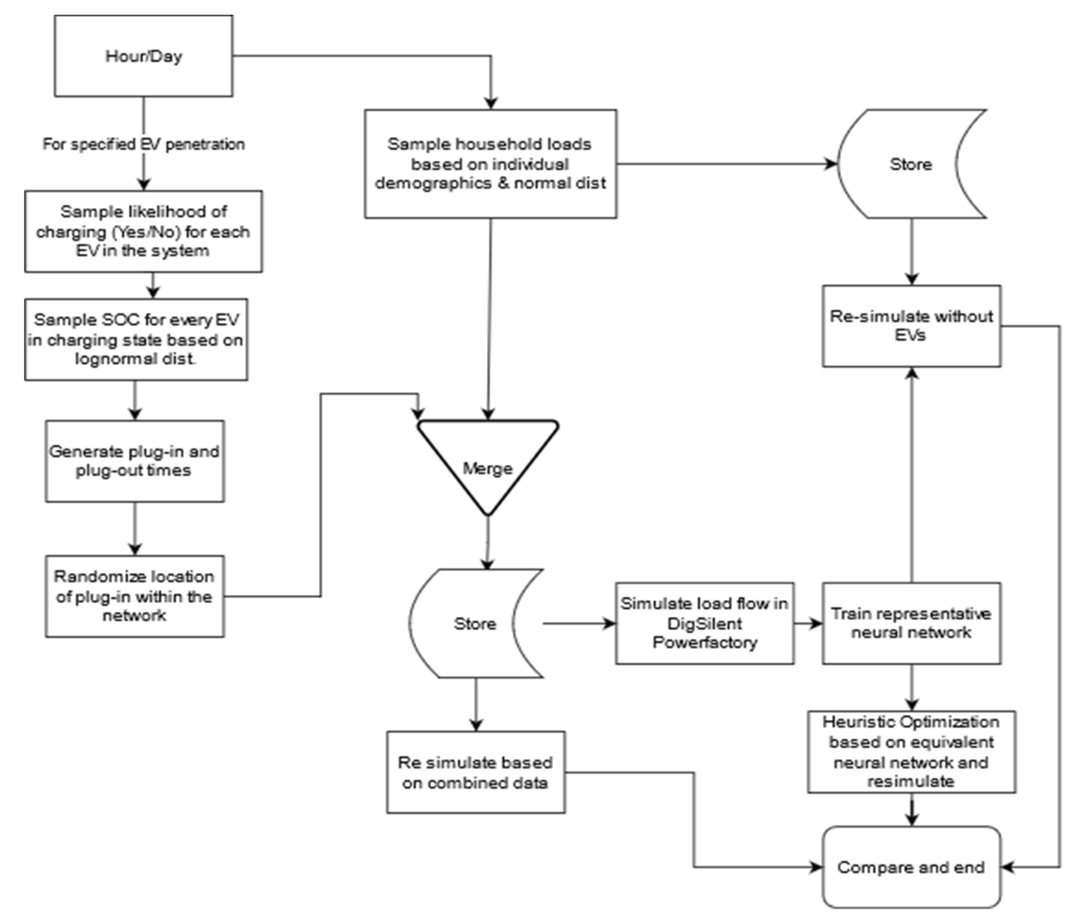
To formulate a Monte-Carlo analysis, typical European consumption behavior was assumed. This was sampled from agent-based modelling from the Load Profile Generator software to simulate electricity consumption [7]. Further explanation of the methodology and corresponding dataset was hosted at [8]. The outputs in the sampled values depend on the population demographics considered previously. From the available scenarios, usage patterns based on population, solar irradiance for distributed generation (DG) and individual car charging behavior were kept constant, based on the footprint of previously discussed European studies [3,4,6,8]. The methodology for simulation was kept constant as in the previous literature; summarized in Figure 1.
For the purpose of this study, the following four low voltage feeders were considered.
- Network 1.
- 10 bus- and 155 house–networks, based on CIGRE European benchmark grid.
This network was discussed in the previous literature that focused on the heuristic optimization of the EV charging configuration based on line loading, voltage drops, and line losses. A simplified grid layout is shown in Figure 2. Key takeaways about the structure of this network include an unbalanced binary tree structure, with the left string being longer than the right. Cable diameters of this network are available in the literature [15,16].
The number of EV’s simulated in this network is summarized in Table 1. This was based on the assumption that approximately half the population of the hypothetical area owns personal vehicles, in line with typical European car ownership statistics [18].
- Network 2.
- Network 2: 20 bus- and 200 house feeders, based on a densely populated apartment complex.
This network was designed on the basis of a typical densely populated city block, based on the map of the New York City. The critical difference between this network and other LV networks was the availability of two identical transformers at the highest potential nodes of the network. The lengths of the cables were identical at 60 m each, and every node was a block of 12 flats rated at 4 kW peak usage, with hourly consumption values being scaled between 0 and 1. Each block was programmed to include sufficient EV charging space for EV penetrations, as shown in Table 2. For comparison purposes, the resolution of simulation was kept constant at 1-hr intervals, as in previous and subsequent networks.
The simplified network diagram is shown in Figure 3. Since the network was densely packed, the distributed generation did not lead to significant changes in results. This was because the buildings in this network were high-rise apartments, with little space available for solar panel installation. Cable numbers were highlighted in individual boxes and were used to specify locations for the consolidation of results.
While the diagram represents the network as having one transformer, they are implemented using two identical transformers connected to one grid interconnection to the medium voltage (MV) level (11 kV). The grid was programmed to act as a ‘slack’ terminal, and adjusts according to the power demands of the network. Transferring electricity back to the MV network is disallowed at this stage.
Across this network, typical population demographics are simulated, including population demographics and usage patterns based on those employed for network 1, based on similar methodology in the literature [8]. This was done to increase uniformity in data and relegate differences in charging effects to be based purely on topological differences between the two networks. Both connected transformers were of the 2.5MVA Yyn6 type with two windings. Every node in this network represented 12 houses and their EV charging space composed of multiple fast-chargers rated at 17.5 kW.
- Network 3.
- 13 bus and 85 house rural feeders based on a grid from Frankfurt-Main.
This network was based on a typical European rural network, composed of a star-shaped topology. Almost every node in this network was directly connected to the main post-transformer terminal, with negligible longitudinal effects of a load on other subsequent possible loads. The topology of the network is shown in a single line diagram in Figure 4.
Individual terminals other than the main one after the transformer in this network are labelled T1–T12, with the cables labelled 1 to 12 accordingly. The network was based on a similar network from Frankfurt/Main used in the literature [20]. The area was characterized by large open spaces, paving the way for higher distributed generation via solar panels. Cable specifications for this network are shown in Table 4. It is important to note that the lengths of the cables are kept constant, while terminals T10 and T12 have a loop structure.
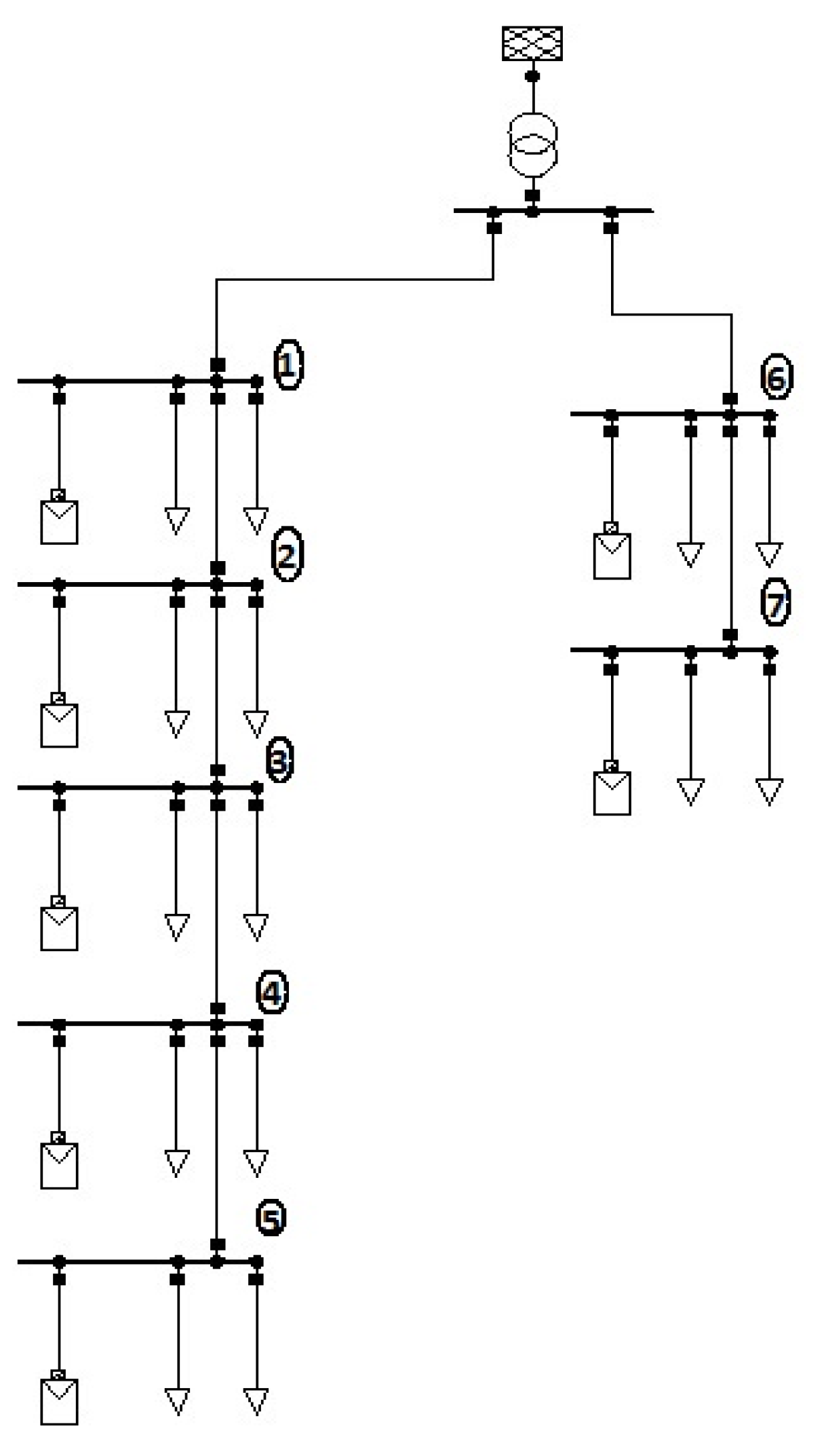
The connected transformer was a 2.5 MVA Yyn6 two-winding transformer. Each EV charging node had at least one 17.5 kW fast charger. Other rated load characteristics of the network are summarized in Table 5. Solar panels and relevant inverter systems were rated at the values specified in Table 5. Every house in this network was allotted multigenerational user characteristics from the literature [8].
The number of houses in this simulation was 85, with the number of EVs varying between 0 and 60 in increments of 15. The user behavior specifications in terms of EV usage were kept constant, as in previous networks. User behavior for individual houses was kept according to the ‘multigenerational’ demographic specified previously [8]. This was different from urban networks that are composed of smaller households with different population demographics representing more variations in the hypothetical population’s age, usage, and relationships.
- Network 4.
- 7 buses and 28 large houses low-voltage network based on a grid from Islamabad.
This network was physically remapped from an anonymized network based in Islamabad. The network incorporates one feeder, composed of 28 houses. Each house is built according to the same specifications using the same material. The population dynamics of each house were multigenerational, with at least 4 occupants per house. Each house was configured with 12 kW solar panels and a corresponding NEPRA license. Since the houses were 90 ft × 100 ft with multiple stories, it was assumed that every house could have between 0 and 2 EVs that might need to charge, as per stochastic properties. Cable properties are as stated in Table 6.
The connected transformer has a rating of 1.25 MVA and has the same datasheet as GEAFOL transformers manufactured by Siemens [21]. A single-phase equivalent diagram of the network is shown in Figure 5 with the cable numbers highlighted.
For every simulation, the mean and standard deviation values for vehicle user behavior as well as solar irradiation were kept constant [3,4], and only variations in topology and network design were allowed to be significantly different between them. For every hour of every day, 106 simulations based on individual household and vehicle user stochastics were run, with data points that lay outside three standard deviations from the mean being removed in order to reduce outliers. All vehicles were assumed to be Tesla model S equivalent with 60 kWh battery packs and a 17.5 kW Tesla fast charger that supplied current according to previously measured statistics [4].
3. Results
3.1. Network 1
Figure A1 shows a heat map showing the expected cable loading observed at various locations of network 1, across a typical day, for varying penetrations of EVs. With no EVs in the network, maximum values observed between 1000 and 2230 hrs was below 60%. No significant overloading was observed with an addition of 30 vehicles, as shown in Figure A1.
With 40 EVs in the network, average line loading in cables 1–3 rose to as high as 80%. It was obvious from the diagram that these cables would require equipment upgrades to increase their carrying capacity, as high EV penetration led to the expected cable loading going up to 200%. Since the peaks of EV charging and household usage did not coincide, a longer rise of 10 h during the day was observed. The difference between the average and worst-case overall line loading observed in the simulation (after removal of outliers) is shown in Figure 6.
Across voltage drops, the results showed a cluster around terminals 7 and 9, which showed acceptable levels of voltage drops at all hours, with EV penetrations of up to 60. Figure A2 shows that the voltage drops were not observed until peak vehicle charging hours with 80 or more EVs. On average, the voltage drops remained within the allowable ranges for most scenarios.
However, the 5% allowable voltage drops level was breached upon introduction of 80 or more EVs in the network. Peak voltage drop was about 20% (line to ground), which coincided with the EV charging peak at hours 1400–1600, as shown in Figure 7.
When observing the average active and reactive power requirements of the feeder, both distributed generation (DG) and no-solar generation scenarios were considered. DG showed significant lowering of peak power requirements by about 100–150 kW. Solar panel introduction had a lesser impact on the reactive power requirements, as shown in Figure 8a,b.
3.2. Network 2
For this network, the average line loading observed across all cables and locations are summarized in Figure A3, versus hour of the day for all EV penetrations. For less than 60 EVs in the network, the “mesh” structure was able to incorporate EVs without reaching its designed capacity. However, for penetrations over 80 EVs, the network was in the worst case, loaded up to 95% across cables 30–35. This showed, however, that no significant equipment upgrades were needed for increasing EV penetrations, purely based on cable loading.
Across all simulations, after removing the outliers, the maximum cable loading observed for 100 EVs reached a little over 100%. On average, the cables had 80–90% unused capacity, as shown in Figure 10.
While the observing voltage dropped across cables, no cable showed a voltage drop greater than 5%, which was the overall upper limit allowed across typical European LV networks. For lower EV penetrations, no significant change in percentage voltage regulation was observed. The maximum observed voltage drop was skewed slightly in the case of 100 EVs, due to the nature of the outliers’ removal, but stayed within the allowed 5% limit, as shown in Figure A4. As expected, terminals lower down in the network experienced more voltage drops compared to the rated line-to-ground voltage.
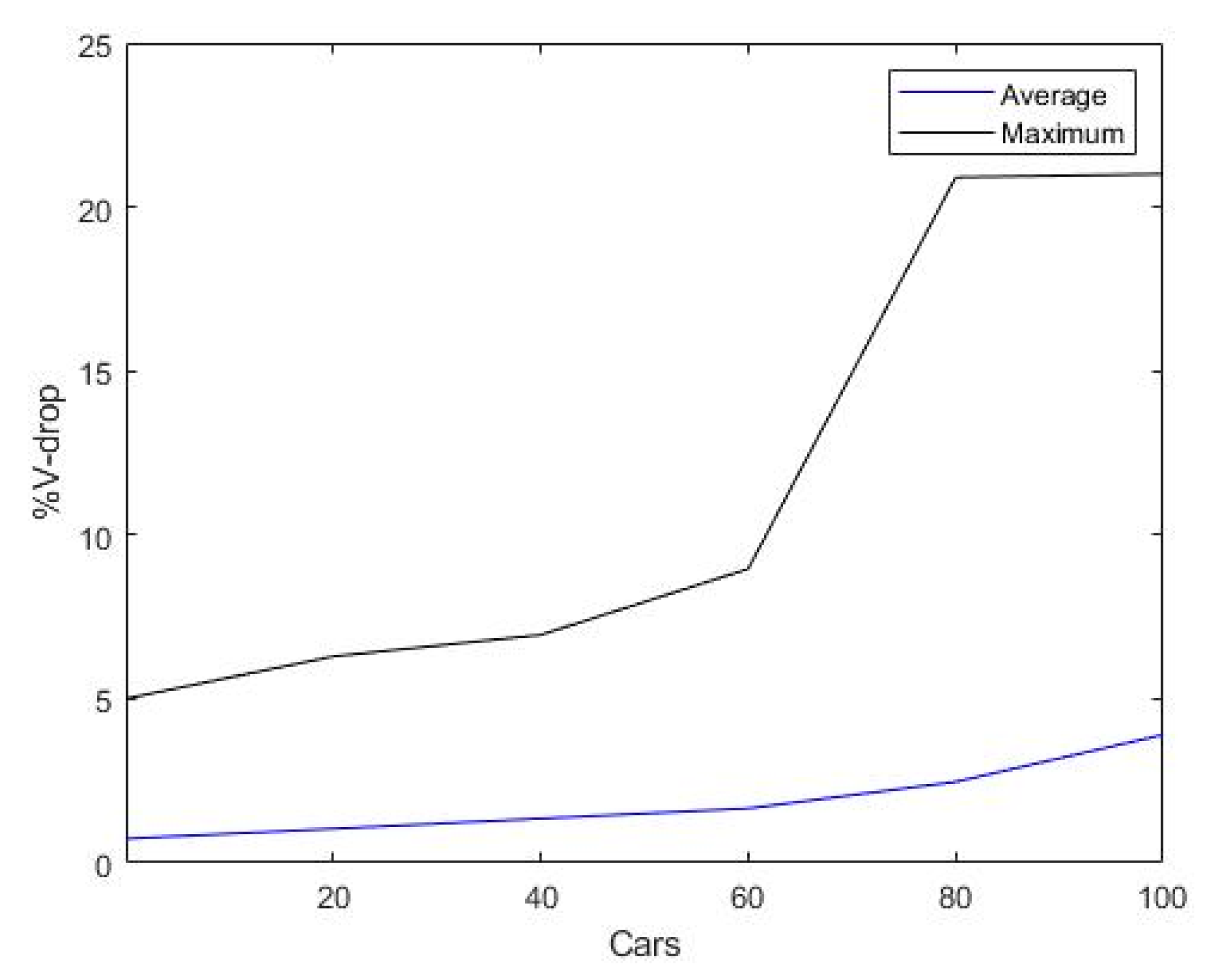
Figure 11 shows the maximum observed percentage voltage drop with respect to EV penetration in black and the average in blue. On average, the voltage drop remained below 1%, whereas even in the maximum values (after removal of outliers in the data), the voltage drop did not exceed 5%. The value for 60 EVs was higher than expected, but was still within the allowable limits.
The current requirements, active power requirements, and reactive power needs of this network under the current simulation conditions are summarized in Figure 12. In the worst case, the network needed a maximum of up to 0.5 kA, which was lowered to 0.3 kA by introducing DG in the network. Similarly, active power requirements dropped from as high as 0.5 MW to 0.3 MW and reactive power from 0.15 MVAR to 0.1 MVAR due to the introduction of DG.
3.3. Network 3
In this network, between 0 and 60 cars were randomly distributed for charging across a day. The aggregated total current demand in the absence of distributed generation (DG) reached 1 kA for the entire network, measured at the primary windings of the transformer. When DG by way of solar panels was allowed, this was lowered to 0.6 kA peak demand. This is shown in Figure 13.
Similarly, peak power consumption of the entire network went up to 500 kW when 60 cars were simulated. For 45 cars and below, the peak active power observed on the transformer level was 0.3 MW and below. Introducing DG allowed the peak power requirements to fall by up to 0.1 MW across the board. The reactive power requirements of the network showed a peak of 0.25 MVAR without DG, and with the introduction of solar power generation, this reduced marginally. This is summarized in Figure 14.
Without the DG being allowed, the maximum observed cable loading percentages ranged from below 20% without any EVs to as high as 100% with 60 EVs charging across one day. For increments of 15 EVs, the maximum observed cable-loading increased by about 15%, respectively, as shown in Figure A5. This showed that under reasonable stochasticity, EV charging in rural networks did not warrant cable upgrades when only looking at the percentage loading across individual cables.
Looking at voltage drops across the network, the longer lengths of the cables in typical rural networks resulted in significant voltage drops in the worst case. Without EVs, the typical voltage drops observed were below 5% of the rated value. However, introducing 30 or more EVs in the network increased the maximum observed voltage drops to 7% and in the worst case, this went as high as 8–9% when 60 EVs were simulated. This is summarized in Figure A6.
When distributed generation was turned on in the simulation, the cable loading percentage dropped slightly on average, with the maximum values reaching the same peaks as before in some scenarios, but being lower by approximately 5%. As this area had a high solar potential and increased access to space to install solar panels, this significantly offset energy demand, but the star topology of this network reduced the direct impact of this on peak cable loading in turn. These results are summarized in Figure A7. Voltage drops across the network showed a peak reduction of 1% in the case of 60 EVs, but were otherwise of a similar magnitude when DG was turned off, barring minor increases as per increases in EV penetration, as shown in Figure A8.
3.4. Network 4
In this network, a small real-world single feeder network in a tree formation. Since this was a smaller network, every node represented 2 houses, with the number of EVs in the simulation assigned to every node being 0, 1, or 2, representing a no-EV case, 50% and 100% EV penetrations, respectively. The allowed values were upper limits that represented how many cars would charge at that node in one day. The actual number of EVs charging at that location was simulated stochastically. The results reflected the multigenerational characteristics mentioned in the literature [8] and the peaks in the afternoon and evening.
Without distributed generation, the network consumed a maximum of 0.05 kA to 0.5 kA for EVs between zero and two. The high solar potential in this region as well as the large size of the installed solar panels resulted in a significant drop in peak current requirements. The worst possible value observed was below 0.05 kA at the transformer level. Current requirements at the transformer level are summarized in Figure 15.
Without DG, peak active power requirements varied from 0.01 MW to 0.2 MW depending on the hour of the day and the number of EVs in the simulation. With up to two EVs allowed to charge at every location, the peak power requirements were significantly higher. At hours 1400 and 1800, the peak power draw was 0.2 MW. Without DG, the peak reactive power requirements observed were up to 0.016 MVAR. Increasing EV penetration did not seem to have a significant effect on this. For active power, the introduction of DG reduced the peak observed value to 0.06 MW. Peak reactive power requirements were lowered to approximately 0.006 MVAR. This is summarized in Figure 16.
Without DG, the peak line loading percentage observed varied from 17% across cables 6–7, to as high as 40% across locations 1–3 in the case of two EVs charging at any location. With DG, however, this difference was lowered to negligible values, as shown in Figure A9. Similarly, without DG, the peak voltage drop was as high as 5% of the rated value when 2 cars were allowed to charge at every location. Without EVs, this was lower with a maximum observed drop of 2%. Increasing EV penetration also aggregated voltage drops around locations 4 and 5 in the network. With DG enabled, this was significantly lowered with the maximum observed V-drop staying below 1.5% across all scenarios. Voltage drops are summarized in Figure A10. Peak cable-loading was observed even with maximum EV penetration; when DG was allowed, this was about 10% of individual cable ratings. A similar case was observed in the case of percentage voltage drop observed across the network.
4. Discussion
Simulating electric vehicles in Low Voltage (LV) networks led to increases in typical network loading parameters. The results were, however, highly dependent on multiple factors such as topology, EV penetration, and usage patterns. For this study, the usage patterns were kept constant across all networks. Typical voltage and line loading percentages for these simulations peaked at the consumer data dependent peak around 1400 hours. These showed variability across different network topologies. Network 1 was dependent on a typical European suburban network. For EV penetrations below 60 cars, it showed the allowable cable loading and voltage drop percentages. However, with 80 or more EVs in the network, the voltage drops went above the 5% limit, with a maximum of 15% observed. This followed the line loading percentage trend, which went as high as over 200% across cables 1–3 during the peak hours of 1100 to 1900. This was due to the inherent density of the network, which had 155 houses spread across a top–down structure with cables 1–3 carrying the most load. The reactive power requirements of the whole feeder totaled a maximum of 0.6 MVAR and the active power maximum reached as high as 0.8 MW. These were both reduced by about 10–20% with the introduction of distributed generation. Distributed generation also slightly offset the peak current drawn by the feeder by about 15%. However, the solar potential in this network was lower, so the DG did not significantly reduce line loading and voltage drop percentages.
Network 2 was a denser network with a compact mesh layout composed of densely packed apartment buildings. The structure was uniform and was connected on two ends by the same grid. This led to smaller household electricity consumption and more equitable cable loading across the network. With 100 cars in the worst-case cable loading peaks at 60–100%, voltage drops were still below the allowed 5% limit. There was no significant change in the power factor values observed. The solar potential of this network was lower than network 1, and therefore, DG was not a significant factor in reducing the loading characteristics. Peak active and reactive power requirements of the network dropped by about 20%, due to the introduction of DG during daytime hours. The current drawn showed a similar trend. Network 3 was a rural network with longer cables, lower number of consumers, and higher solar potential. This led to up to 50% lower aggregate maximum current drawn, with active power and reactive power maximum values being 40% lower than the maximums, before the introduction of DG. Maximum cable loading without DG was always lower than 80% with up to 60 EVs in the network. Voltage drops were above the 5% limit, with a maximum voltage drop of 7% due to 60 EVs in the worst case. The introduction of large swathes of solar panels lowered both these values significantly, with the maximum voltage drop reaching the allowed 5% limit. DG introduction also significantly reduced the peak current requirements and active power requirements of the feeder. This was typical of rural networks in economically richer communities with significant rural potential.
Network 4 was unique in the sense that it was the only network based on a community in a developing country, which led to a constraint-rich environment. The sizes of the houses in this network were significantly larger, with EV penetration being higher due to the smaller size of this network. Overall, it showed similar voltage drop percentages as network 3, but a large solar panel generation as that of a real-world network was introduced, this was reduced to almost negligible. The installed cables were rated higher than necessary, so the peak cable loading was never found to rise above 30% even without DG.
5. Conclusions
The simulations led to a highly topology-dependent outcome. Urban areas are slated to have more issues dealing with cable loading percentages, while semi-urban and rural networks are observed to have more issues related to voltage drops across the network. It was also observed that there was a significant gap between peak power and current usage values during off-peak and peak hours of the day, which led to a greater potential of smarter charging of EVs, increasing their use as storage sinks to offset the “duck curve” of electricity production from distributed generation [22]. Network 4 in particular showed great potential for islanding as well, and if implemented properly via the vehicle-to-grid (V2G) methodology, this community showed significant potential to survive as an islanded micro-grid during typical load-shedding hours.
The values presented in this study should be used as a dataset that could be aggregated at the medium voltage (MV) level, to summarize low voltage networks and project them to one node. This would reduce the overall computational complexity for subsequent analyses of larger networks. Furthermore, the networks should then be optimized using heuristic methods, as presented in [4], to find optimal charging configurations. A heuristic approach for such networks could also be used to find the optimal solutions for power injection back into the network, to minimize the effects of overloading. This could be used for vehicle-to-grid methods, where the overloading caused by EVs could be minimized using unused EVs instead of moving the load to a different time slot or through equipment upgrades. The authors propose that future work in this area should focus on the potential solutions to some of the overloading observed in the urban and semi urban networks mentioned in this paper and in the literature. Solutions like equipment upgrades, charging placement optimization, reactive and active power injection, could be used in conjunction with V2G, to lower the entry barrier faced by EVs in the network. Key takeaways from this study include the need to optimize vehicle charging in both time and space. Furthermore, the authors propose the introduction of a spatial distribution surcharge on the cost of electricity available to individual consumers within the LV network, to compensate for the individual effects that every charging location has on the network. Networks with longer strings composed of uniform cabling should make the cost of charging EVs higher at farther connections in the linear network. Alternatively, different networks should also take into account their specific cable diameters when accounting for this surcharge. Older networks with smaller cable diameters downstream have unintuitive cable overloading patterns observed. Further studies on the medium and high voltage levels could use the aggregated active power, current, reactive power, and power-factor values presented for these different LV networks as load profiles to reduce overall computational complexity as well. While the two stochastic datasets upon which user behavior is based on in this simulation coincidentally align with each other and with solar generation, future studies should include more diverse studies to incorporate contradictory scenarios as well, such as an LV network with night-time wind power generation versus daytime household and EV usage.
Author Contributions
Literature search, S.H.; data curation and creation, S.H.; methodology design, S.H. and P.S.; data validation, S.H.; simulation and results consolidation, S.H.; Supervision, P.S.; revisions and proofreading, P.S. Both authors have read and agreed to the published version of the manuscript.
Funding
This research was made possible by the funding provided by the Boysen–TU Dresden Research Training Group. Open Access Funding by the Publication Fund of the TU Dresden.
Data Availability Statement
Data available online. Haider, Sajjad (2021), “Data related to simulation of varying EV penetrations in LV grids”, Mendeley Data, V1, doi:10.17632/kw6yt7ykdc.1.
Conflicts of Interest
The authors declare no conflict of interest.
Appendix A
Figure A1.
Maximum line loading (percentage) observed in network 1.

Figure A2.
Peak voltage drops (percentage) observed in the network 1—plotted against terminal location and time of the day.
Figure A2.
Peak voltage drops (percentage) observed in the network 1—plotted against terminal location and time of the day.

Appendix B
Figure A3.
Maximum cable loading (percentage) observed across network 2 over varying EV penetration and time of day.
Figure A3.
Maximum cable loading (percentage) observed across network 2 over varying EV penetration and time of day.

Figure A4.
Maximum voltage drops (percentage) observed across network 2 by varying EV penetration and time of day.
Figure A4.
Maximum voltage drops (percentage) observed across network 2 by varying EV penetration and time of day.

Appendix C
Figure A5.
Maximum cable loading (percentage) observed in network 3 with distributed generation OFF.
Figure A5.
Maximum cable loading (percentage) observed in network 3 with distributed generation OFF.

Figure A6.
Maximum voltage drops (percentage) observed in network 3 with distributed generation OFF.
Figure A6.
Maximum voltage drops (percentage) observed in network 3 with distributed generation OFF.

Figure A7.
Maximum line loading (percentage) observed in network 3 with distributed generation ON.

Figure A8.
Maximum voltage drops (percentage) observed in network 3 with distributed generation ON.

Appendix D
Figure A9.
Maximum observed line loading (percentage) across the entire network (network 4) with and without distributed generation (DG).
Figure A9.
Maximum observed line loading (percentage) across the entire network (network 4) with and without distributed generation (DG).

Figure A10.
Maximum observed voltage drops (percentage) across the entire network (network 4), with and without distributed generation (DG).
Figure A10.
Maximum observed voltage drops (percentage) across the entire network (network 4), with and without distributed generation (DG).

References
- Widén, J.; Lundh, M.; Vassileva, I.; Dahlquist, E.; Ellegård, K.; Wäckelgård, E. Constructing load profiles for household electricity and hot water from time-use data—Modelling approach and validation. Energy Build. 2009, 41, 753–768. [Google Scholar] [CrossRef]
- Liao, F.; Molin, E.; Van Wee, B. Consumer preferences for electric vehicles: A literature review. Transp. Rev. 2016, 37, 252–275. [Google Scholar] [CrossRef] [Green Version]
- Schäuble, J.; Kaschub, T.; Ensslen, A.; Jochem, P.; Fichtner, W. Generating electric vehicle load profiles from em-pirical data of three EV fleets in Southwest Germany. J. Clean. Prod. 2017, 150, 253–266. [Google Scholar] [CrossRef] [Green Version]
- Haider, S.; Schegner, P. Heuristic Optimization of Overloading Due to Electric Vehicles in a Low Voltage Grid. Energies 2020, 13, 6069. [Google Scholar] [CrossRef]
- Gautam, D.S.; Musavi, F.; Edington, M.; Eberle, W.; Dunford, W.G. An Automotive Onboard 3.3-kW Battery Charger for PHEV Application. IEEE Trans. Veh. Technol. 2012, 61, 3466–3474. [Google Scholar] [CrossRef]
- Pflugradt, N. Modellierung von Wasser-Und Energieverbräuchen in Haushalten. 2016. Available online: https://nbn-resolving.org/urn:nbn:de:bsz:ch1-qucosa-209036 (accessed on 19 April 2021).
- Pflugradt, N.; Muntwyler, U. Synthesizing residential load profiles using behavior simulation. Energy Procedia 2017, 122, 655–660. [Google Scholar] [CrossRef]
- Haider, S.; Schegner, P. Data for Heuristic Optimization of Electric Vehicles’ Charging Configuration Based on Loading Parameters. Data 2020, 5, 102. [Google Scholar] [CrossRef]
- Al-Alawi, B.M.; Bradley, T.H. Review of hybrid, plug-in hybrid, and electric vehicle market modeling Studies. Renew. Sustain. Energy Rev. 2013, 21, 190–203. [Google Scholar] [CrossRef]
- Ensslen, A.; Will, C.; Jochem, P. Simulating electric vehicle diffusion and charging activities in France and Ger-many. World Electr. Veh. J. 2019, 10, 73. [Google Scholar] [CrossRef] [Green Version]
- Sachan, S.; Deb, S.; Singh, S.N. Different charging infrastructures along with smart charging strategies for electric vehicles. Sustain. Cities Soc. 2020, 60, 102238. [Google Scholar] [CrossRef]
- Huang, S.; Infield, D. The impact of domestic Plug-in Hybrid Electric Vehicles on power distribution system loads. In Proceedings of the 2010 International Conference on Power System Technology, Zhejiang, China, 24–28 October 2010; Institute of Electrical and Electronics Engineers (IEEE): Piscataway, NJ, USA, 2010; pp. 1–7. [Google Scholar]
- Wang, Y.; Infield, D. Markov Chain Monte Carlo simulation of electric vehicle use for network integration studies. Int. J. Electr. Power Energy Syst. 2018, 99, 85–94. [Google Scholar] [CrossRef]
- Fischer, D.; Harbrecht, A.; Surmann, A.; McKenna, R. Electric vehicles’ impacts on residential electric local profiles—A stochastic modelling approach considering socio-economic, behavioural and spatial factors. Appl. Energy 2019, 233–234, 644–658. [Google Scholar] [CrossRef]
- Faessler, B.; Schuler, M.; Preißinger, M.; Kepplinger, P. Battery storage systems as grid-balancing measure in low-voltage distribution grids with distributed generation. Energies 2017, 10, 2161. [Google Scholar] [CrossRef] [Green Version]
- Haider, S. Data for optimization of Electric Vehicle charging configuration to reduce overloading in low voltage networks. Mendeley Data 2020, 102. [Google Scholar] [CrossRef]
- Strunz, K.; Abbasi, E.; Fletcher, R.; Hatziargyriou, N.; Iravani, R.; Joos, G. Benchmark Systems for Network Integration of Renewable and Distributed Energy Resources; Cigre: Paris, France, 2014. [Google Scholar]
- Guo, Z. Residential Street Parking and Car Ownership. J. Am. Plan. Assoc. 2013, 79, 32–48. [Google Scholar] [CrossRef]
- Graupner, H. Cars Still Rule the Roost in Germany. DW, 2018. Available online: https://www.dw.com/en/cars-still-rule-the-roost-in-germany/a-46289162 (accessed on 12 August 2020).
- Neusel-lange, N.; Zdrallek, M.; Oerter, C.; Germany, M.A.G.; Uhlig, R.; Stiegler, M. Economic Evaluation of Dis-Tribution Grid Automation Systems—Case Study in A Rural German Lv-Grid Lv-Grid Automation System Cired Workshop; Cired Workshop: Rome, Italy, 12 June 2014; Paper 0054, no. 0054; pp. 11–12. [Google Scholar]
- Siemens, A.G. GEAFOL Cast-Resin Transformers 100 to 16000 kVA, 2007. Available online: https://www.quad-industry.com/titan_img/ecatalog/GEAFOL100-16000kVA.pdf (accessed on 19 April 2021).
- Denholm, P.; O’Connell, M.; Brinkman, G.; Jorgenson, J. Overgeneration from Solar Energy in California: A Field Guide to the Duck Chart (NREL/TP-6A20-65023); Technical Report; National Renewable Energy Lab. (NREL): Golden, CO, USA, 2015. [Google Scholar]
Figure 1.
Methodology to generate EV charging models and calculate plug-in and out times based on Monte-Carlo simulation. The methodology is similar to those presented in the literature, and is kept constant across all simulations in this paper [4].
Figure 1.
Methodology to generate EV charging models and calculate plug-in and out times based on Monte-Carlo simulation. The methodology is similar to those presented in the literature, and is kept constant across all simulations in this paper [4].

Figure 2.
Single-line diagram of LV network based on the CIGRE benchmark grid showing 10 terminals with individual loads representing different numbers of houses and charging locations [8,17].

Figure 3.
Line diagram showing layout of network 2 with cable characteristics summarized in Table 3. The network is uniform in terms of the rated sizes of the nodes, cable diameters, and lengths.
Figure 3.
Line diagram showing layout of network 2 with cable characteristics summarized in Table 3. The network is uniform in terms of the rated sizes of the nodes, cable diameters, and lengths.

Figure 4.
Line diagram showing layout of network 3. The network is in a star topology centered at the terminal connected to the secondary winding of the transformer.
Figure 4.
Line diagram showing layout of network 3. The network is in a star topology centered at the terminal connected to the secondary winding of the transformer.

Figure 5.
Single-line diagram showing cable layout of network 4 showing the 7 terminals with 14 connected houses as well as the aggregated solar panel installations.
Figure 5.
Single-line diagram showing cable layout of network 4 showing the 7 terminals with 14 connected houses as well as the aggregated solar panel installations.

Figure 6.
Maximum line loading (percentage) observed in the network versus average observed across all cables when plotted against EV penetration.
Figure 6.
Maximum line loading (percentage) observed in the network versus average observed across all cables when plotted against EV penetration.

Figure 7.
Maximum voltage drops (percentage) observed in the network versus average observed for all terminals when plotted against the EV penetration.
Figure 7.
Maximum voltage drops (percentage) observed in the network versus average observed for all terminals when plotted against the EV penetration.

Figure 8.
(a) Maximum active power requirements of the complete network v. (b) Maximum reactive power requirements of the peak network. Both values are aggregated at the primary windings of the transformer and plotted against EV penetration.
Figure 8.
(a) Maximum active power requirements of the complete network v. (b) Maximum reactive power requirements of the peak network. Both values are aggregated at the primary windings of the transformer and plotted against EV penetration.

Figure 9.
Maximum current requirements of the complete network aggregated at the primary windings of the transformer and plotted against EV penetration.
Figure 9.
Maximum current requirements of the complete network aggregated at the primary windings of the transformer and plotted against EV penetration.

Figure 10.
Maximum single cable loading (percentage) observed across the network over varying EV penetration vs. average cable loading plotted against EV penetration.
Figure 10.
Maximum single cable loading (percentage) observed across the network over varying EV penetration vs. average cable loading plotted against EV penetration.

Figure 11.
Maximum voltage drop (percentage) observed across the network over varying EV penetration versus the average voltage drop.
Figure 11.
Maximum voltage drop (percentage) observed across the network over varying EV penetration versus the average voltage drop.

Figure 12.
(a) Maximum current drawn by the feeder. (b) Peak active power requirements of the network. (c) Peak reactive power requirements of the network versus EV penetration.
Figure 12.
(a) Maximum current drawn by the feeder. (b) Peak active power requirements of the network. (c) Peak reactive power requirements of the network versus EV penetration.

Figure 13.
Maximum current requirements observed across the network over varying EV penetration with and without distributed generation (DG).
Figure 13.
Maximum current requirements observed across the network over varying EV penetration with and without distributed generation (DG).

Figure 14.
(a) Maximum active power requirements of the complete network. (b) Maximum reactive power requirements of the peak network.
Figure 14.
(a) Maximum active power requirements of the complete network. (b) Maximum reactive power requirements of the peak network.


Figure 15.
Total current requirements for the entire network versus the number of allowed cars across every two houses.
Figure 15.
Total current requirements for the entire network versus the number of allowed cars across every two houses.

Figure 16.
Total active power requirement (MW) of the entire network vs. total reactive power requirement (MVAR) of the entire network.
Figure 16.
Total active power requirement (MW) of the entire network vs. total reactive power requirement (MVAR) of the entire network.


Table 1.
EV penetration scenarios for network 1 [19].
Table 1.
EV penetration scenarios for network 1 [19].
| No. of Cars in Simulation | No. of Houses without Cars | Vehicle Penetration % |
|---|---|---|
| 0 | 200 | 0 |
| 20 | 180 | ~20% |
| 40 | 160 | ~40% |
| 60 | 140 | ~60% |
| 80 | 120 | ~80% |
| 100 | 100 | ~100% |
Table 2.
EV penetration scenarios for network 2.
| No of Cars in Simulation | Number of Houses without Cars | Vehicle Penetration [18] % |
|---|---|---|
| 0 | 200 | 0 |
| 20 | 180 | ~20% |
| 40 | 160 | ~45% |
| 60 | 140 | ~67% |
| 80 | 120 | ~89% |
| 100 | 100 | ~111% |
Table 3.
Cable characteristics of network 2.
| Cable No | Cable Type | Underground Rated Current (kA) | AC-Resistance (Ohm/km) | Reactance X’ (Ohm/km) | Length (m) | Cross-Sectional Area (m2) |
|---|---|---|---|---|---|---|
| 32–35 | NA2XY | 0.455 | 0.102 | 0.069 | 60 | 300 |
| 1–31 | NA2XY | 0.400 | 0.127 | 0.069 | 60 | 120 |
Table 4.
Cable characteristics for network 3.
| Cable No | Cable Type | Underground Rated Current (kA) | AC-Resistance (Ohm/km) | Reactance X’ (Ohm/km) | Length (m) | Cross-Sectional Area (m2) |
|---|---|---|---|---|---|---|
| 1–12 | NA2XY 3 Core | 0.155 | 0.642 | 0.072 | 400 | 50 |
Table 5.
Terminal rated peak active power, reactive power, and solar generation characteristics.
| Terminal | Active Power P kW | Reactive Power Q kVAR | Rated Solar P kW |
|---|---|---|---|
| 1 | 20 | 4 | 30 |
| 2 | 16 | 3.6 | 26 |
| 3 | 52 | 12 | 32 |
| 4 | 24 | 6 | 0 |
| 5 | 36 | 9 | 0 |
| 6 | 36 | 9 | 22 |
| 7 | 40 | 9 | 0 |
| 8 | 44 | 10 | 0 |
| 9 | 28 | 7 | 20 |
| 10 | 32 | 8 | 32 |
| 11 | 8 | 2 | 0 |
| 12 | 4 | 1 | 54 |
Table 6.
Cable characteristics for network 4.
| Cable No | Cable Type | Underground Rated Current (kA) | AC-Resistance (Ohm/km) | Reactance X’ (Ohm/km) | Length (m) | Cross-Sectional Area (m2) |
|---|---|---|---|---|---|---|
| 1 | NYY | 0.478 | 0.100 | 0.184 | 100 | 185 |
| 2 | NYY | 0.363 | 0.126 | 0.091 | 100 | 150 |
| 3 | NYY | 0.323 | 0.154 | 0.092 | 100 | 120 |
| 4 | NYY | 0.284 | 0.194 | 0.095 | 100 | 95 |
| 5 | NYY | 0.237 | 0.269 | 0.098 | 100 | 70 |
| 6 | NYY | 0.237 | 0.269 | 0.098 | 100 | 70 |
| 7 | NYY | 0.237 | 0.269 | 0.098 | 100 | 70 |
Publisher’s Note: MDPI stays neutral with regard to jurisdictional claims in published maps and institutional affiliations. |
© 2021 by the authors. Licensee MDPI, Basel, Switzerland. This article is an open access article distributed under the terms and conditions of the Creative Commons Attribution (CC BY) license (https://creativecommons.org/licenses/by/4.0/).
Share and Cite
MDPI and ACS Style
Haider, S.; Schegner, P. Simulating the Impacts of Uncontrolled Electric Vehicle Charging in Low Voltage Grids. Energies 2021, 14, 2330. https://0-doi-org.brum.beds.ac.uk/10.3390/en14082330
AMA Style
Haider S, Schegner P. Simulating the Impacts of Uncontrolled Electric Vehicle Charging in Low Voltage Grids. Energies. 2021; 14(8):2330. https://0-doi-org.brum.beds.ac.uk/10.3390/en14082330
Chicago/Turabian StyleHaider, Sajjad, and Peter Schegner. 2021. "Simulating the Impacts of Uncontrolled Electric Vehicle Charging in Low Voltage Grids" Energies 14, no. 8: 2330. https://0-doi-org.brum.beds.ac.uk/10.3390/en14082330
Note that from the first issue of 2016, this journal uses article numbers instead of page numbers. See further details here.