
Decarbonization of Residential Building Energy Supply: Impact of Cogeneration System Performance on Energy, Environment, and Economics †


Buildings and Transportation Science Division, Oak Ridge National Laboratory, 1 Bethel Valley Road, Oak Ridge, TN 37830, USA
†
This manuscript has been authored by UT-Battelle, LLC under Contract No. DE-AC05-00OR22725 with the U.S. Department of Energy. The United States Government retains and the publisher, by accepting the article for publication, acknowledges that the United States Government retains a non-exclusive, paid-up, irrevoca-ble, world-wide license to publish or reproduce the published form of this manuscript, or allow others to do so, for United States Government purposes. The Department of Energy will provide public access to these re-sults of federally sponsored research in accordance with the DOE Public Access Plan (http://energy.gov/downloads/doe-public-access-plan ).
Energies 2021, 14(9), 2538; https://0-doi-org.brum.beds.ac.uk/10.3390/en14092538
Submission received: 7 April 2021
/
Revised: 21 April 2021
/
Accepted: 25 April 2021
/
Published: 28 April 2021
(This article belongs to the Special Issue Micro-Combined Heating, Cooling, and Power Systems for Buildings: State-of-the-Art, Commercialization Challenges, and Research Opportunities)
Abstract
:Electrical and thermal loads of residential buildings present a unique opportunity for onsite power generation, and concomitant thermal energy generation, storage, and utilization, to decrease primary energy consumption and carbon dioxide intensity. This approach also improves resiliency and ability to address peak load burden effectively. Demand response programs and grid-interactive buildings are also essential to meet the energy needs of the 21st century while addressing climate impact. Given the significance of the scale of building energy consumption, this study investigates how cogeneration systems influence the primary energy consumption and carbon footprint in residential buildings. The impact of onsite power generation capacity, its electrical and thermal efficiency, and its cost, on total primary energy consumption, equivalent carbon dioxide emissions, operating expenditure, and, most importantly, thermal and electrical energy balance, is presented. The conditions at which a cogeneration approach loses its advantage as an energy efficient residential resource are identified as a function of electrical grid’s carbon footprint and primary energy efficiency. Compared to a heat pump heating system with a coefficient of performance (COP) of three, a 0.5 kW cogeneration system with 40% electrical efficiency is shown to lose its environmental benefit if the electrical grid’s carbon dioxide intensity falls below 0.4 kg CO2 per kWh electricity.
1. Introduction
The global energy demand is ever increasing and administrations are trying to use precious energy resources as effectively as possible while, at the same time, aiding the increased penetration of renewable energy in realizing low/zero carbon economy [1]. Recent increases in wind and solar energy generating capacity have done much to reduce the reliance on carbon fuels, but an important complementary strategy is using available energy resources more efficiently. Chemical energy’s potential in meeting the growing energy demand is indisputable. Fuels such as biogas [2], hydrogen [3], natural gas (NG) [4] and propane (LPG) are considered to play the role of bridging resources while we shift towards 100% clean energy. Technological solutions are necessary to utilize readily available resources (e.g., fuels) with the highest possible conversion efficiency [5]. Cogeneration technologies are capable of delivering usable energy to the end consumer at a higher efficiency than the traditional method of separate electric and thermal production. Yet, this strength is typically unexploited in building applications due to the disparity between production versus consumption, thermal-to-electrical energy ratio, cost, and electrical efficiency [6]. The cogeneration system’s effectiveness in converting fuel’s chemical energy to useful electrical and thermal energy at the desired ratio and quantity plays a substantial role in building application. Fuel-based hybrid power systems can lessen a building’s primary energy and carbon dioxide burden, and augment energy resiliency if the total useful energy (both as power and waste heat) is completely utilized onsite [7]. The concurrent electrical and thermal energy generation at a high efficiency from an onsite fuel source can lower a building’s greenhouse gas (GHG) discharge [8]. Such an approach can lower transmission losses while also addressing surges in energy demand and helping in grid stabilization. Cogeneration-based distributed energy resources, in conjunction with digital technologies, can further enable higher primary energy efficiency and lower carbon footprint via smart energy management strategies, data-driven grid information and communication technologies, and connected devices. The principal factors for enabling broadscale adoption of cogeneration products include resiliency, low/zero carbon footprint, retrofittability, cost competitiveness, and lower energy in buildings [9].
1.1. Relevant Work
The prime movers (PM) taken into consideration [10] for such purposes comprise conventional and emerging power systems. Internal combustion engine (ICE)-based cogeneration equipment has been the most researched technology.
Mahian et al. employed the Grey Wolf Optimizer for optimizing a diesel generator-PV-wind turbine-battery system with a focus towards cost optimization [11]. Similarly, Fazelpour et al. investigated a 150 kW diesel generator-PV-wind turbine hybrid hardware for multi-family residential building with the objective of lowering the price of electricity [12]. A multi-PM design strategy employing three ICE-based cogeneration systems for meeting the needs of 20 users has been shown to lower the fuel consumption compared to single equipment-based design [13]. Energy charge savings via hydrogen blended natural gas in a 5 kWel ICE-based micro-CHP was investigated and reported by Santoli et al. [14]. Other heat engine-based cogeneration systems investigated included heat engines such as stirling (SE) [15], micro gas (MGT) [16] and steam turbines (MST) [17], suitable for a multi-family dwelling application.
Substitute electrochemical technologies, for instance, fuel cells were also investigated for building applications. Ellamla et al. presented a comprehensive assessment of fuel cell cogeneration equipment status in different countries [18]. Real time optimization methodology was adopted to maximize fuel utilization, via the load following approach, in an 8 kW constant load residential building [19]. Detailed system configuration analysis of a hybridized version with a heat pump system suggested primary energy savings when utilizing a 1 kWel fuel cell [20].
One kWel Solid Oxide Fuel Cell (SOFC) system with and without load modulation was modeled and analyzed for its techno-economic performance when employed in a residential building cogeneration application [21]. A Polymer Electrolyte Membrane fuel cell (PEM) was also modeled for optimizing the integration with residential buildings’ heating and domestic hot water thermal equipment [22]. Similarly, Ito et al. presented a detailed economic and environmental assessment of a residential 0.7 kWel PEM cogeneration system [23]. This method was shown to provide environmental benefits even if the electrical grid’s carbon intensity level was 0.2 kg/kWhel. Cost and performance analysis of a hybrid heat pump plus PEM cogeneration system was recently reported [24], where the authors concluded economic and energy benefits of deploying a heat pump in conjunction with a fuel cell. A hybrid PEM-absorption chiller-based cogeneration system was modeled and analyzed for residential buildings where 30% energy savings were reported [25]. Other emerging technologies investigated included: Flame Fuel Cells (FFC) [26], Thermophotovoltaic (TPV) [27,28], Thermoelectric (TE) [29], Thermionic Emission (TIE) [30], and Organic Rankine Cycle (ORC) [31]. Modeling of a combined solar, geothermal, ORC-based polygeneration energy system was recently reported [32]. This configuration was shown to lower primary energy and carbon intensity by greater than 94% and 97%, respectively, with an estimated payback of >16 years. Similarly, Calise et al. examined the performance of a combined solar, geothermal and ORC-based trigeneration system [33], where the inclusion of energy storage on economics and energy balance was studied and reported.
The fuel-to-electric output efficiency of such PM technologies varies widely, by up to 50%, while the thermal-to-electrical output (T/E) ratios fluctuate by up to 15. A detailed analysis of different PM technologies was recently assessed based on the key attributes of cost, cycling, emissions, capacity, and technical and commercial feasibility [34].
In this context, energy modeling of the cogeneration system helps optimize the system capacity and fit while improving the evaluation and simulation of cogeneration system implementation in a building. A comprehensive overview of various modeling approaches adopted by international researchers was recently reported [35]. This study presented the advanced thermodynamic models and their benefits. Additionally, model improvement strategies to enhance their applicability in a wide range of energy architectures were also presented. Cogeneration equipment fueled by fossil and renewable sources, along with different prime movers including heat engines, renewable power sources and electrochemical power sources, were reviewed from a wide range of modeling approaches including an Annex 42-based approach [36]. Roselli et al. recently reported dynamic simulations suitable for techno-environmental assessment of cogeneration equipment [37]. This study investigated the impact of central power plant efficiency variation on the onsite trigeneration system’s value proposition in different geographical regions. The significance of power plant efficiency was highlighted, and a particular cogeneration approach offered significantly different energy savings. Evolution of the energy architecture was also considered in the cost and performance analysis of a trigeneration system in supporting conventional electrical and thermal loads along with that of electric vehicles [38]. Dynamic simulations using 5 kWel micro-cogeneration hardware in conjunction with boiler and chiller suitable for a multi-story building was conducted with the TRNSYS software platform. This study highlighted the primary energy savings and carbon dioxide emissions reduction with the cogeneration approach while compared to several other examined configurations, with and without PM.
1.2. Problem Statement
Although the benefits of installing a resilient cogeneration device on site are well understood, the optimal size of such a system, and the sensitivities associated with the heat-to-power ratio, electrical efficiency and power rating for residential building applications, are still unclear. Numerous investigations suggested a wide range of electrical power ratings [10] for residential scale PM, varying from 1.5 kW [39] to 5 kW [14] for ICE-based systems, 0.65 kW [31] to 7 kW [40] for ORC-based devices, 5 kW [17] with a MST device, 0.7 kW [18] to 6 kW [19] for FC-based systems, and up to 250 W using TE/TPV devices [29,31]. As can be seen, there is a high degree of variance in the electrical efficiency and the suggested electrical power rating of the cogeneration system when applied in different residential environments. One of the reasons for such a noteworthy variance in the rated power output is the operational strategy, electrical efficiency, and continuous vs. intermittent operation of the PM. Electrical and thermal energy storage capacity also play a substantial role in the observed sizing variance.
Due to the energy efficiency impact of cogeneration, numerous researchers, technology developers and equipment manufacturers are targeting residential applications (21% of total US energy consumption) [41]. Designing a cogeneration system that fulfills the building’s energy requirements is a challenging proposition as the seasonal and time-of-day variances of power and heat load change considerably. The residential building’s energy needs are chiefly influenced by the ambient conditions in a particular region, while the E/T ratio can fluctuate from up to 3.5 [42]. This is largely driven by the heat load oscillation from 30 Btu to 60 Btu per square feet [43]. In addition to the technical compatibility, another important aspect associated with such approach is the cost, which greatly influences the acceptance at a broader scale.
1.3. Motivation and Contribution
Given the substantial role of cogeneration in addressing the energy and environmental burden of buildings, the primary objective of the present study is to investigate the impact of different design characteristics on key technical and economic metrics. Decarbonization of buildings in the context of this paper refers to lowering or elimination of the carbon footprint or carbon dioxide emissions (GHG) associated with electrical and thermal energy demand by the building. GHG emissions caused by energy consumption (both at the source and at the site) are the target of the present study. A comprehensive analysis of the influence of generator power rating, its electrical and thermal efficiency, and its cost, (capital and maintenance) on lifetime electrical grid purchases, total primary energy consumption, overall carbon dioxide footprint, operating expenditure, return on investment (ROI, measure of profitability), and, most importantly, thermal vs. electrical energy balance, is presented. The main objective is to help the readers envisage varying influencing characteristics and their impact on a product’s cost, energy, and environmental benefits, and finally, utility bill savings for the end user. Amongst many factors which can influence the broad scale adoption of energy-efficient solutions, cost premium and energy/environmental benefits are important to consider when designing a residential building-specific cogeneration. The capacity of the battery, power rating of the PM, physical size, and operational and maintenance costs, need to be minimized to lower the capital expenditure and enhance ease of integration with existing building stock.
In this framework, design specification to lower the (i) the primary energy consumption, (ii) electrical grid purchases, (iii) annual operational energy and (iv) carbon dioxide emissions, without producing excess thermal or electrical energy, but supplementing the building energy needs at a low cost while enhancing the energy resiliency and efficiency using an onsite cogeneration, is investigated and presented in this work.
The rest of the paper is dedicated to a detailed explanation of the (i) approach utilized, including assumptions and calculations performed, (ii) case studies evaluating different design configurations and (iii) conclusions outlining favorable configurations that meet the objectives mentioned above.
2. Approach
The influence of different configurational aspects on key performance and cost attributes was studied in detail. The primary variables considered for each design configuration included: (i) power rating, (ii) electrical efficiency, (iii) auxiliary renewable power source (photovoltaic, PV), (iv) unit cost, and (v) electrical grid’s carbon intensity. The key attributes that were investigated included: (i) total primary energy, (ii) electrical grid purchases, (iii) excess thermal and electrical production, (iv) utility bill savings, (v) annual carbon dioxide emissions reductions, (vi) ROI, and (vii) payback period. Natural gas was considered as the primary fuel for the cogeneration system. These operational variables and resulting economic, environmental and performance metrics were investigated for residential buildings.
2.1. Methodology
Modeling of the hybrid energy configuration was conducted using commercial simulation software, HOMER® Grid (version 1.7, Homer Energy by UL, Boulder, USA) [44]. This software package combines engineering and economics information in one comprehensive model. Complex calculations comparing multiple components and design outcomes are performed to identify points at which different technologies become cost competitive. The optimization algorithm simplifies the design process by identifying least cost configurations while considering the configurational aspects (described above) of each application layout. The simulation process identifies each configuration’s performance as a function of time. The principal objective of the optimization process is to reduce peak power purchases from the utility by determining the best mix of resources for the least-cost solution and highest possible rate of return while considering the configurational aspects of each application layout and satisfying the technical constraints of peak power and total energy. The dispatch strategy picks the best economic option for serving the load at each time step by considering the tariff, weather, and available power component in each configuration. Details related to simulation, optimization, energy management and dispatch strategies are very well presented [45,46].
A brief overview of various components and how they are utilized in the simulation model is described here. HOMER’s principal strength is simulation of a power generation system-based cogeneration configuration over the lifecycle. HOMER streamlines and optimizes onsite energy generation technology in both supplemental and islanding scenarios through user-selectable customizable components. HOMER’s simulation and optimization strategy, along with impact analysis of different parameters, enables assessment of the cost and performance viability of several combinations of configurational elements by considering differences in equipment price and accessibility to each energy provider. At its core, HOMER simulates a feasible method for blending each energy configurational element imposed by the user. All analyzed configurations are organized consistently, with distinct conditions chosen by the user as an economic or fuel optimization model. Sensitivity analysis allows modeling of the impact of such variables as fuel price, PM electrical efficiency, the grid’s carbon dioxide factor, etc., and assesses the ways in which the best configuration changes with these differences. A list of key components and their boundary conditions and parameters utilized in this study are outlined in table below. The package allows the user to choose a tariff from a central database or simply define the fixed energy charges along with utility’s carbon dioxide burden expressed as grams per unit of electricity generated. The electric load can be imported from a time series file containing data of 365 consecutive days. The thermal energy needs are met by a standard boiler, an electrical power generator or by surplus electricity. For each prime mover under consideration, a percentage thermal recuperation value defines the value of useful thermal energy to meet the thermal load in each timestep while supplemented by a boiler with defined efficiency, if needed. The simulation software accounts for the complete conversion of all of the fuel chemical energy into electrical and thermal output. The PM’s fuel consumption correlation stipulates useful electrical output for the supplied amount of fuel while the balance is accounted for as thermal energy production after considering the heat recuperation ratio. In addition, HOMER prioritizes the energy source at each time step by considering the electrical demand and the cost aspects of the PM versus other available power providers. However, in the present study, the PM was assumed to operate all the time by forcing the schedule option in the software for 100% availability. Several storage models based on idealized and kinetic models can be utilized for electrical energy management. The energy storage module considers similar losses during both charging and discharging states while taking into account the user-selectable round-trip efficiency (DC-to-charge-to-DC). The module also allows the user to select a minimum charge threshold after which the available energy is not utilized in serving the load profile. The software also allows usage of a boiler in configurations involving thermal loads, as investigated in this study. HOMER optimizes and identifies the lowest cost solution in supporting the imposed load. The boiler module operates whenever the heat recovery from the PM is insufficient in serving the thermal profile. Photovoltaic modules are implemented in the configuration via user-defined cost structure, electrical bus type and the output derating factor, along with lifetime. In addition, the software package applies Solar Global Horizontal Irradiation (GHI) Resource to compute electrical output from the photovoltaics, based on the location input or through a time-series file. The output from the simulation provides information related to economics, energy price, energy consumption, energy generation by different components, fuel consumption, and emissions. Detailed information related to base case architecture (configuration with lowest net present value), and all other possible configurations setup by the user, is generated. The following values for each possible configuration are provided in the model (as outlined in Table 1): (i) Cost—net present cost, price of electricity, capital cost, operating cost, fuel cost; (ii) Configuration—total annual fuel consumption, annual electrical and thermal energy production (kWh/yr), annual electrical and thermal consumption, excess electrical and thermal production, annual carbon dioxide emission (kg/yr); (iii) Economics—ROI, simple payback, utility bill savings ($/yr), demand charge savings ($/yr), energy charge savings ($/yr); (iv) Individual component—capital cost, energy production (kWh/yr), fuel consumption (if utilized), autonomy (hours of grid independent operation, e.g., for a battery); (v) Grid/utility—energy purchased and sold (kWh), demand cost, energy cost ($). Additionally, the program also generates time series data of the model variables from these simulation results with the same granularity as that of the time-step used in the simulation model, with options including scatter plot (variable comparison), delta plot (frequency of changes in any variable versus time), DMap (concise way to view entire year of data for the selected parameter), profile (hourly performance for an average day for each month for the selected parameter), histogram, cumulative distribution function, and duration curve.
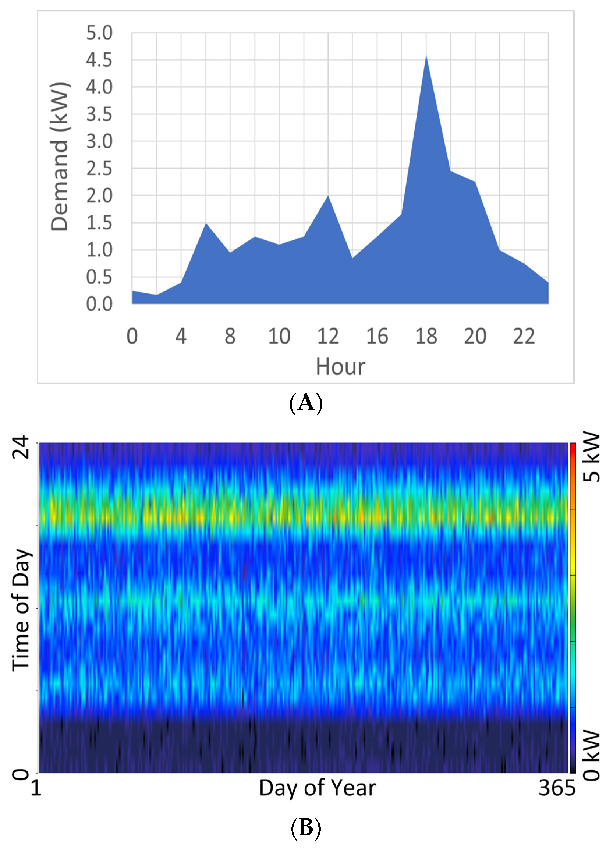
The load profile considered in residential buildings included total average energy consumption of 25 kilowatt-hours per day with a peak load of ~4.5 kilowatt (combined electrical and thermal loads). These values are based on the average energy consumption numbers provided by U.S. Energy Information Administration (EIA, Washington, DC, USA) [47,48]. As shown in Figure 1, the generic load profile is meant to represent the peak demand profile rather than a particular building type and actual consumption in a specific geographical region. Figure 1, for instance, displays the total load as a function of time of the day along with peak consumption periods during the course of the day.
The power source consisted of a technology-agnostic, generic, customized AC power-producing device with a pre-defined electrical output and efficiency (both thermal recovery and electrical efficiency). No specific PM technology was considered as the primary motivation was to study the sensitivity of power rating and energy conversion ratio on benefits to the end user. The power source is assumed to operate continuously since one of the objectives of this study is to minimize the kW rating of the power source module to lower the capital cost as well as physical footprint. This mode of operation and power range may not be suitable for some of the available PMs but fits very well with technologies such as fuel cells, TPV, thermionic, and thermoelectric devices. Electrical efficiency of the PM (fuel heating value to electrical power output) was also modulated between 25% and 50% [49]. Thermionic emission-based PM, fuel cell, stirling engine, and ICE-based configurations typically achieve this efficiency range. Different power outputs from 0.1 kW to 1 kW were created in the software as customized power source modules.
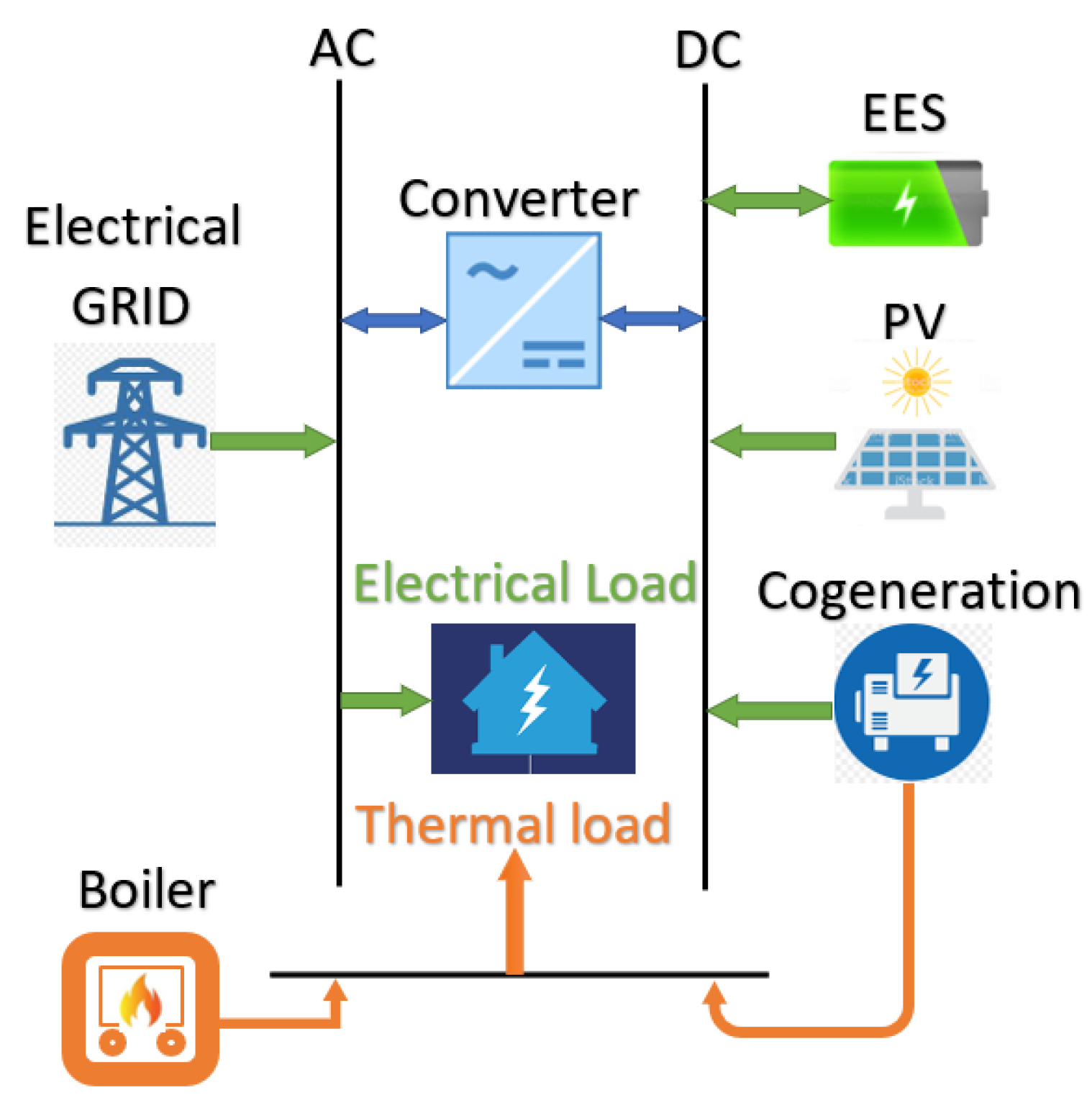
The hybrid energy architecture considered for this analysis involved an (i) electrical battery module (2 kWh battery, 4000 kWh lifetime throughput), (ii) a boiler serving the thermal load via natural gas (85% efficient) after utilizing the heat recovered from the power source (if needed), (iii) an optional auxiliary PV power source, and (iv) a converter (95% efficient), as shown in Figure 2. Additional thermal energy storage was not considered in this analysis as the goal was to minimize the excess energy production and the boiler utilized will act as the on demand thermal provider, essentially acting as a thermal storage hardware. As shown in the schematic, power sources such as electrical grid, generator and PV are shown as connected to the alternating current (AC) bus while battery resides on the direct current (DC) bus. The direction of energy flow between the source and the consumer is shown along with the load profile type and daily energy consumption rating. The software prioritizes electrical power utilization in the order of primary load on the same bus, followed by the energy storage module, before finally being sold to the electrical grid.
The software evaluates each configuration via accounting for complete energy balance in each time step (20-min interval). A comparison between the electric load and the available energy in each time step is performed, followed by calculation of the energy transfer between all generation and consumption components. In the battery-based configurations, the optimization engine decides in each time step whether to charge or discharge the battery based on the economic impact of the energy available in that time step, with the overall objective of operational cost minimization. A determination on whether a configuration is feasible in meeting the electric load under the conditions specified is made, followed by estimating the price of life cycle costs of the hardware. Additionally, the random variability inputs on electric and thermal loads improves the arbitrariness of the load profile, reflecting realistic conditions.
Each configuration’s life cycle costs are calculated from the capital, maintenance, operating and other economic information such as discount rate and interest. The program also calculates excess electric and thermal energy produced, which is defined as surplus energy not consumed by energy storage or the load profile. This is an important consideration for the presented analysis as the objective is to minimize the excess energy production. The load profiles are accessed from the Open Energy Information database [50], while the tariff related rate structure information is accessed from the Genability database [51]. If PV is employed in the hybrid energy configuration, the solar global horizontal irradiation (GHI) resource is utilized either from NASA (Prediction of Worldwide Energy Resource, POWER) [52] or the National Renewable Energy Laboratory’s Solar Radiation database [53], all built into the software program.
2.2. Assumptions
All assumptions for different configurational elements considered in this analysis are summarized in Table 2.
The building’s daily electrical and thermal loads were assumed to be 15 kWh/day and 10–30 kWh/day, respectively. The average electrical load (true electrical needs) in the USA ranges from 10 kWh/day to 20 kWh/day [60,65]. Therefore, the selected 15 kWh/day is a good representation of the majority of the residential buildings. However, the thermal load varies significantly across the region. The assumed 10–30 kWh/day of thermal load definitely fits the domestic hot water thermal energy needs (typically varies between 7 and 26 kWh/day) across the region [65]. Buildings located in warm-mild climate regions can benefit from the chosen thermal load value. However, cold climate regions’ peak thermal loads can exceed 100 kWh/day [65], in which case the chosen range can only supplement a portion of the load during the peak consumption period. Investment tax credit (30% of capital cost) and bonus depreciation incentive (50% in first year at a marginal tax rate of 21%) were considered for PV, if utilized in the configuration. The cost of electricity (COE) was assumed to be $0.15/kWh, while a net metering cost of $0.1/kWh was considered, and the net operating expenditure reported here is adjusted for any such revenue. The cost of natural gas was assumed to be $0.3/m3. The power source did not take into account any tax credits or incentives. The COP of the heat pump-based thermal comfort hardware, defined as the ratio of useful thermal energy versus electrical consumption, was assumed to be 3.0, while that of electrical heating equipment (resistive heating equipment) was considered as 1.0.
2.3. Calculations
Carbon dioxide emissions are calculated based on the carbon factor (kg of CO2 emitted per unit of fuel consumed) for the electrical grid supply and the local fuel consumption associated with both the cogeneration system’s PM as well as the boiler. Annual emissions are calculated by multiplying the carbon factor (CO2,grid for utility purchases (MWhgrid/yr) and CO2,fuel for natural gas consumption (m3/yr)) by the total annual fuel consumption and MWh purchased from the electrical grid, according to Equation (1).
Operational expenditure savings ($savings, opex) are calculated by comparing the net expenses associated with on-site fuel consumption (m3/yr), net metering revenue (via electric sales to grid, kWhsales) and reduced utility purchases (kWhgrid/yr) with that of the baseline configuration electrical grid as the primary energy source, (kWhbaseline), as shown in Equation (2).
ROI, defined according to Equation (3), is a comparison between annual cash flow versus incremental capital cost difference during the lifecycle of the system installed. In this equation, Lproj is project lifetime, $i,base is yearly cash flow for reference system, $i and $cap are the annual economic benefit and capital expenses associated with the configuration being investigated, and $cap,base is the baseline system’s capital expenditure.
3. Results and Discussion
Based on the assumptions and methodology described in the previous section, a detailed performance analysis was conducted for residential buildings. The key configurational aspects investigated include prime power rating and presence of PV, while the electrical efficiency and cost were the key variables.
3.1. Prime Mover Power Rating
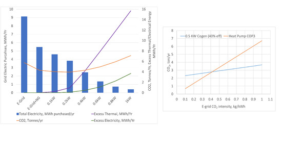
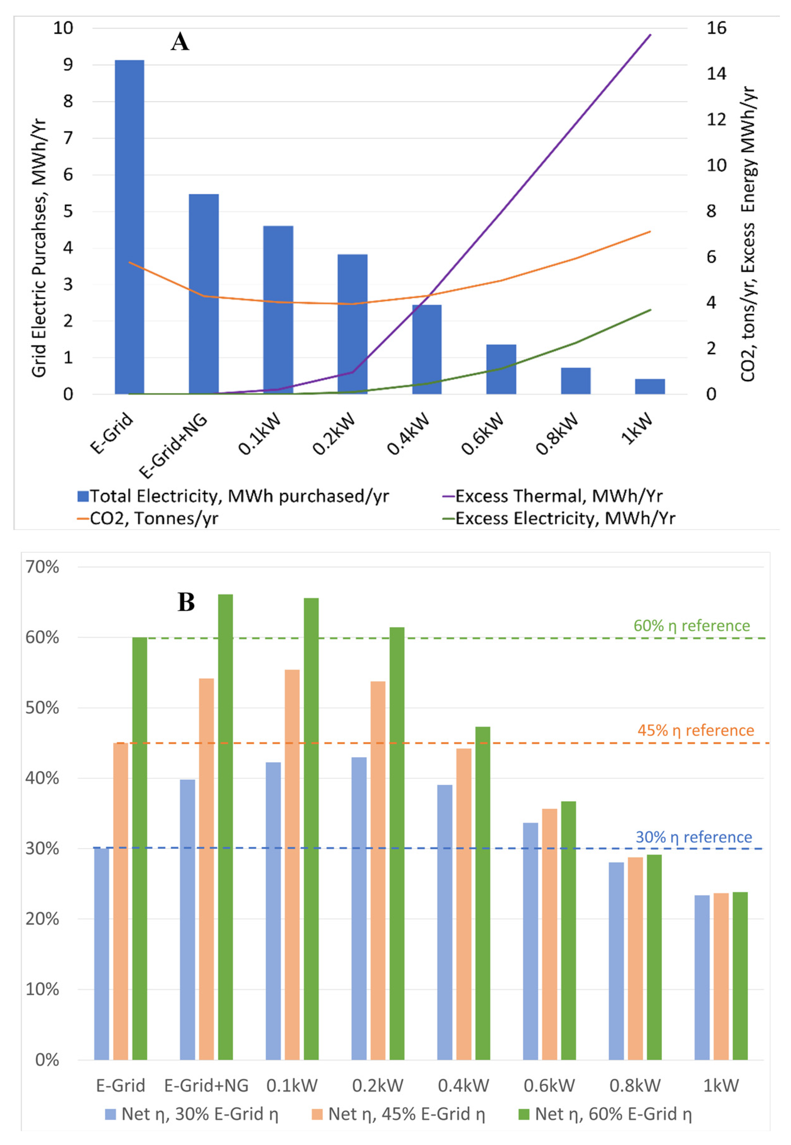
The impact of the cogeneration system’s prime power rating on total annual electrical grid purchases supporting a 25 kWh/day (15 kWh electric, 10 kWh thermal) load is shown in Figure 3A. The cogeneration configuration considered a power generator with a 0.1 kW to 1 kW rating and no auxiliary PV. Electrical efficiency of the PM was assumed to be 25% (defined as electrical power produced vs. fuel heating value of 53.6 MJ/kg) while heat recovery efficiency was assumed as 75%. As shown, the electric grid demand (E-Grid) exceeds 9 MWh/year and decreases to ~5.6 MWh/year if the total thermal load is supported via natural gas. Addition of the cogeneration equipment further decreases the grid demand from ~4.6 MWh/year (with 0.1 kW PM) to <0.5 MWh/year (with 1 kW PM), due to onsite power generation and thermal energy utilization. The excess thermal and electric power generation, while utilizing different PM power ratings, is also shown in the figure. It has to be noted that the electrical battery module size is only 2 kWh. As a result, any excess energy produced beyond the storage capacity and the demand from the load profile is considered as unutilized. It is important to consider this excess energy as it provides the necessary information to optimally size the kW rating of the cogeneration system. As shown in the figure, a 0.4 kW PM produces negligible excess electricity, but it produces excess thermal energy beyond the thermal load profile. Conversely, a 0.2 kW cogeneration system produces negligible excess energy. A power rating beyond 0.4 kW produces excess thermal and electrical energy, as shown in the figure. Sizing these energy storage modules appropriately will decrease the E-grid demand further and utilizes the produced energy efficiently; however, higher capacities increase the capital costs. Additionally, the kW rating has a significant influence on the overall CO2 footprint. E-grid as the primary energy source produces 5.7 metric tons/year of CO2 (assuming a carbon dioxide factor of 0.63 kg CO2/kWh electric power [66]). Utilization of a natural gas boiler for thermal needs decreases this CO2 footprint to 4.3 tons/year. The presence of 0.1 and 0.2 kW cogeneration system further decreases the CO2 emissions to ~4 tons/year. A power rating beyond 0.8 kW yields > 5.7 tons/year, higher than the electrical configuration. Figure 3B displays the combined energy efficiency of each configuration with and without cogeneration equipment while considering different E-grid power plant efficiencies in the range of 30–60% (assuming Natural gas energy density of 53.6 MJ/kg). This analysis will help recognize the overall impact of a cogeneration system’s kW rating on combined energy efficiency in supporting the 25 kWh/day load of a building. The E-grid energy efficiency varies widely across different regions and it is important to analyze the influence of onsite power generation since one configuration/power rating may not fit across all regions. As can be noticed in the figure, a PM size of up to 0.6 kW offers higher efficiency compared to a 30% efficient E-Grid, while it decreases to only 0.4 kW when integrated in a 45% efficient E-Grid scenario. Installation of cogeneration equipment in a region with a 60% energy-efficient E-grid is favorable at onsite cogeneration capacities of up to 0.2 kW only.
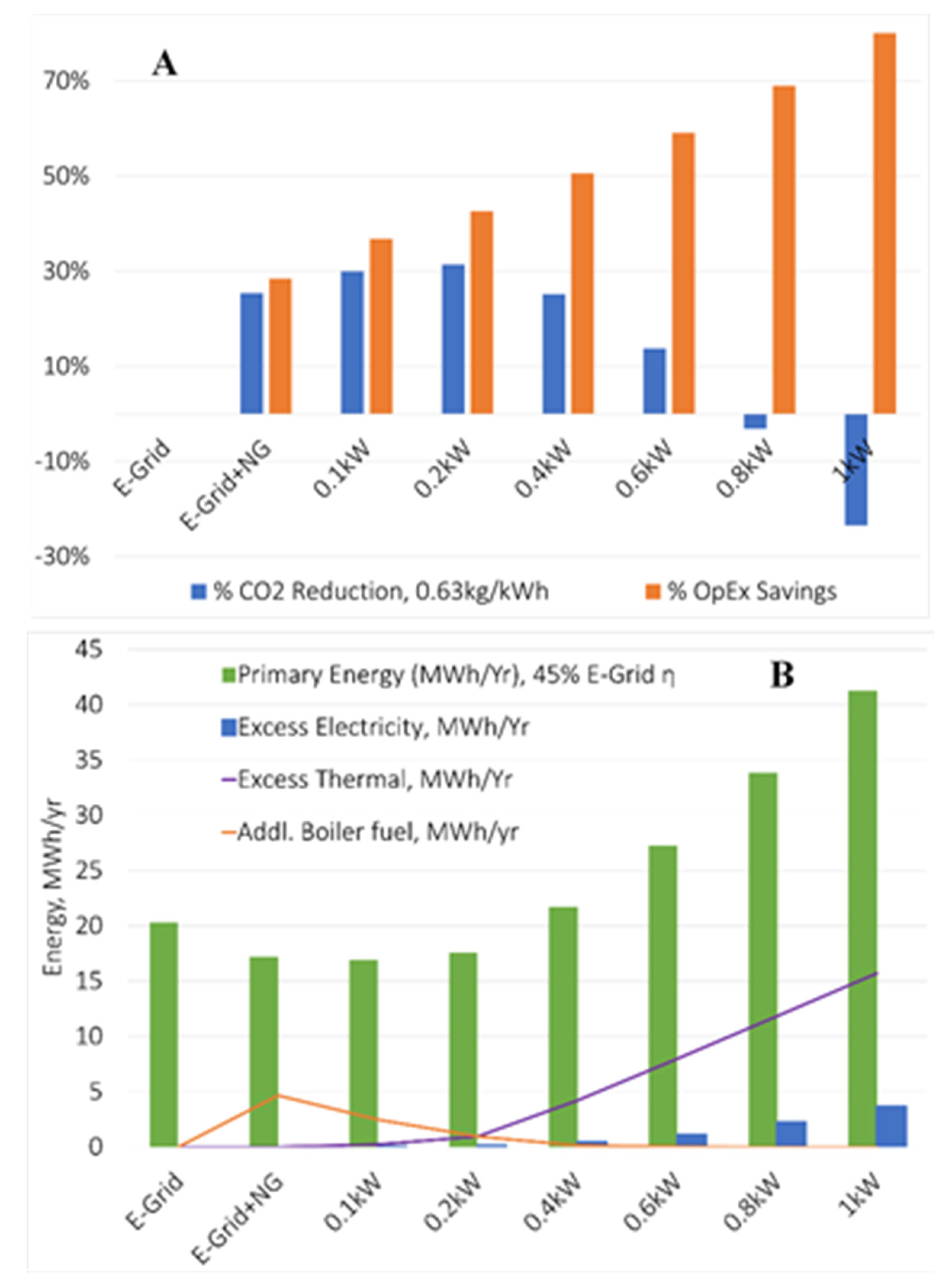
The analysis presented above sheds light on the influence of cogeneration systems from an energy and efficiency perspective, but it is also important to comprehend the economic and environmental benefits. Figure 4A compares the percentage decrease in total carbon dioxide emissions and operational expenditure for different energy configurations discussed above. CO2 emissions can be curtailed by >32% with a 0.1 or 0.2 kW PM and by up to 25% and 15% with a 0.4 kW and 0.6 kW configuration, respectively. However, the higher kW configurations show a negative impact on CO2 emissions since the electrical efficiency of the PM was assumed to be only 25%, which is reflected as excess thermal energy in Figure 4B. It must be noted that the CO2 emissions are not normalized for the total kWh of energy produced (excess electrical and thermal) but rather considered for just the 25 kWh/day useful energy consumption in the building. These values would be improved by a few percentage points if the excess thermal energy is stored and utilized.
Installation of the cogeneration system also results in operational energy cost savings of up to 80%, as shown in Figure 4, mainly driven by the lower price of natural gas and the waste heat produced by the PM in supporting the thermal load, which otherwise would have been supported by E-grid. The operational cost savings presented here account for the excess electricity produced via net metering at a cost of $0.1/kWh. Figure 4B also displays the total primary energy, defined as the combined kWh energy associated with the electrical grid and fuel. The primary energy was calculated after taking into account the energy consumed at the source/generation. A 45% central power plant electrical energy efficiency was assumed for the E-grid portion of the energy supply to the building while a 92% efficiency factor was assumed for the natural gas supply (to account for distribution losses) [67]. As shown, the primary energy consumption of hybrid E-grid/NG configurations of up to 0.2 kW is lower compared to the E-grid only energy supply. In addition, deploying >0.4 kW PM does not require additional natural gas fuel to support the thermal load, but higher power output (>0.4 kW) from the cogeneration system also produces excess thermal and electric energy. The difference in additional boiler fuel and excess thermal energy reflects the thermal balance if a thermal storage component is included in the configuration. For instance, for the 0.2 kW system in Figure 4B, the additional boiler fuel and excess thermal energy converge, implying that the system is thermally balanced if a thermal storage unit is employed.
3.2. Prime Mover Electrical Efficiency
In light of the above discussion where the economic and environmental benefits are observed, the sensitivity of PM’s electrical efficiency was also investigated. A case study was conducted for a high energy efficiency scenario with a building consuming 28 kWh/day, 0.4 kW PM onsite, 0.5 kW renewable power source (PV), and a two kilowatt-hour energy storage module in Oak Ridge, TN, USA. The heat recovery efficiency was set at 75%. Figure 5, Figure 6 and Figure 7 compare the total energy requirement, efficiency and performance, along with CO2 and cost implications, when deployed with varying degrees of PM’s electrical efficiencies.
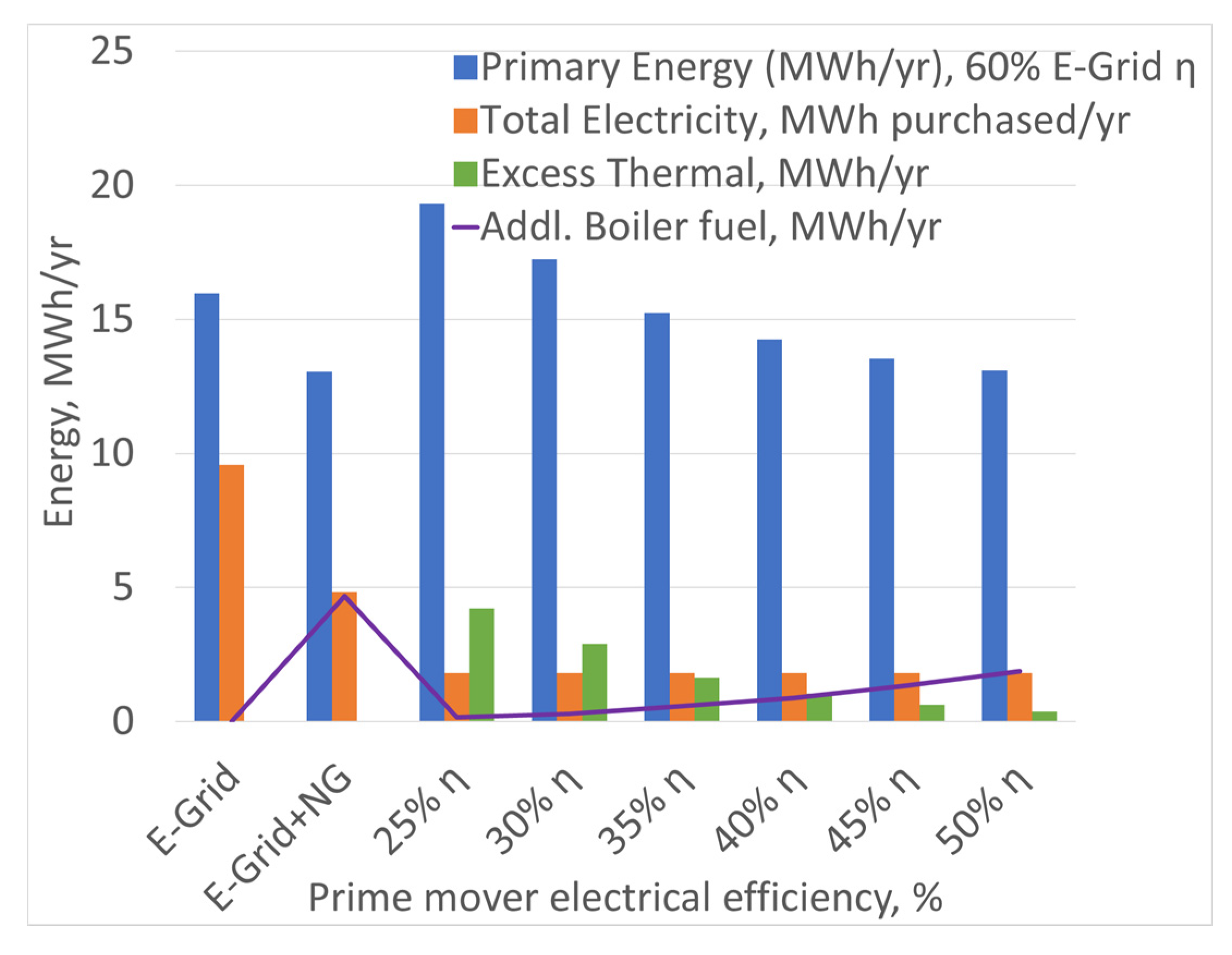
Figure 5 displays the primary energy consumed with an all-electric configuration and hybrid natural gas boiler plus E-grid, with and without a cogeneration system. The E-Grid efficiency was assumed to be 60% while the delivered natural gas efficiency was assumed to be 92%. It can be noticed that the 0.4 kW-based cogeneration approach consumes less primary energy (combined electric plus natural gas at source) when the electrical efficiency is ≥35%. In addition, total E-grid purchases are substantially lower with the cogeneration system (~80% lower compared with all-electric primary energy source). Additionally, as expected, excess thermal energy and total fuel consumption decreases with an increase in the electrical efficiency. The demand for additional boiler heating fuel, however, increases, (in other words, the additional thermal energy needed that is not provided by the 0.4 kW PM) if the electrical efficiency of the PM is above 30%, as can be realized in the difference between additional boiler fuel and the excess thermal energy.
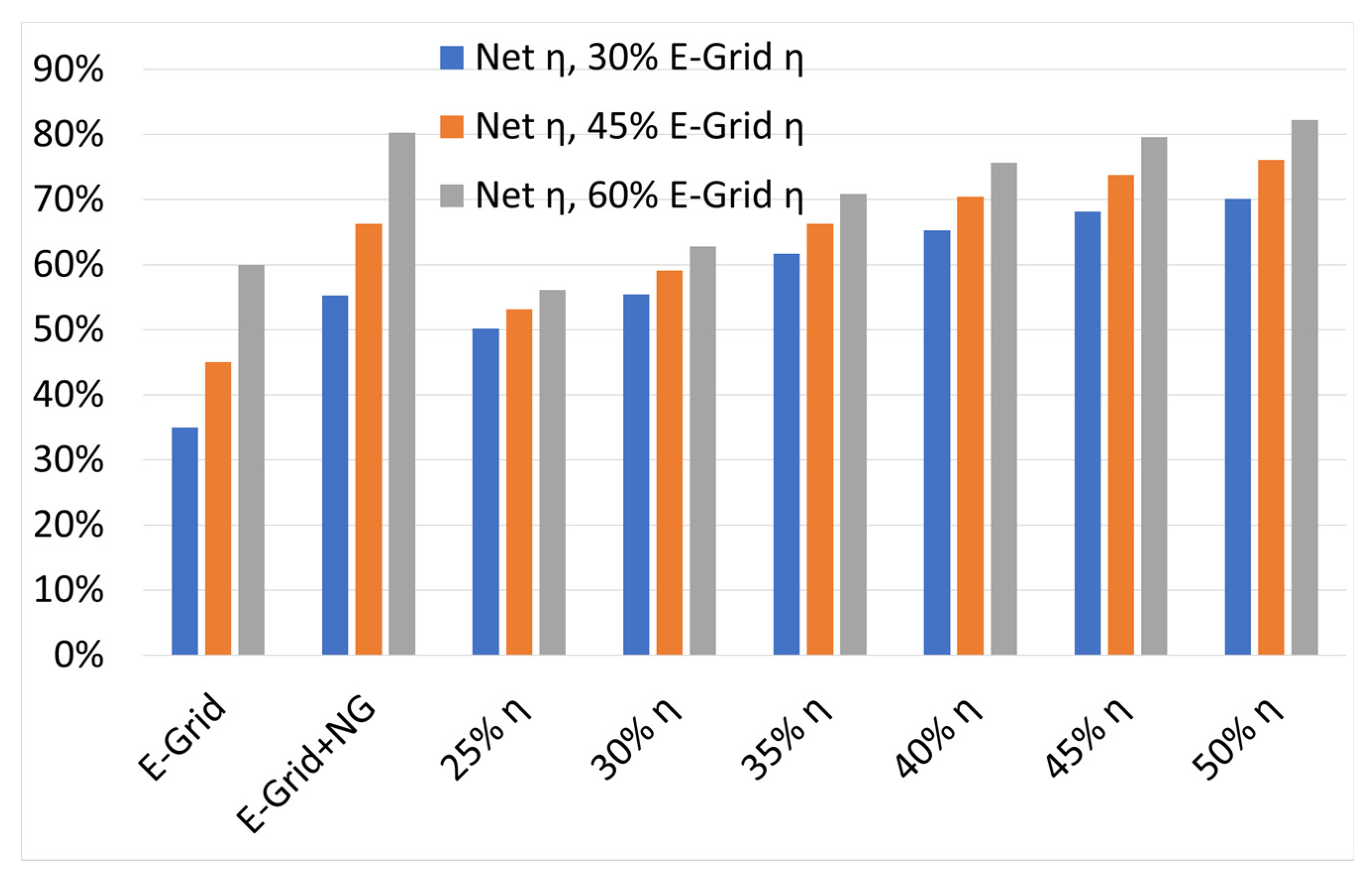
Figure 6 shows a comparison of total energy efficiency of each configuration (all with 0.5 kW PV) while supplementing electrical grid with energy efficiencies of 35%, 45%, and 60%. As displayed, fuel-supported configurations exceed the E-grid-based configuration at efficiencies of 35% and 45%. However, above 60% electrical grid efficiency, the cogeneration configuration must surpass at least 35% electrical efficiency to provide energy benefits.
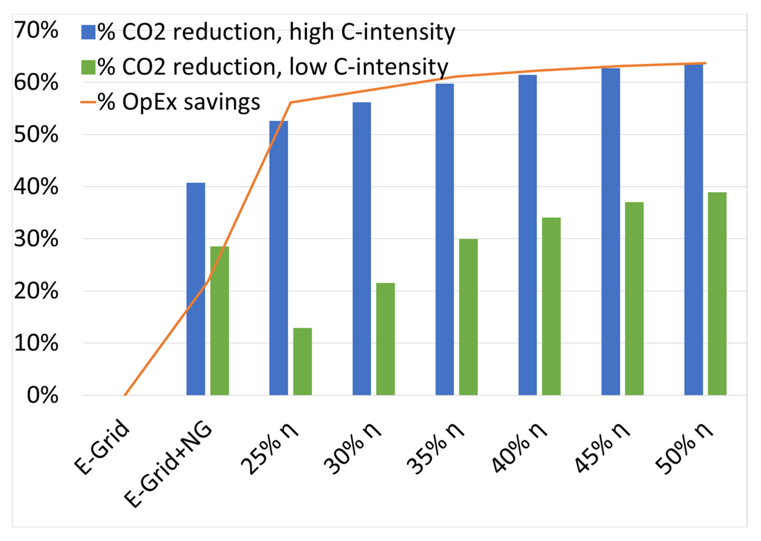
In addition to the energy benefits, the impact of the cogeneration system’s electrical efficiency on the operational expenditure and carbon dioxide footprint was also evaluated. As displayed in Figure 7, two different E-grid sources representing low and high carbon intensities of 0.42 kg CO2/kWh and 1.004 kg CO2/kWh electric production [66], respectively, were considered. It can be noticed that natural gas cogeneration system configurations show > 53% reduction in CO2 emissions if the grid electric supply is from a high carbon intensity power plant. However, compared to low carbon intensity power plants (i.e., high penetration of renewable resources), the cogeneration system’s impact on CO2 reduction is less effective, yielding < 39% reductions. The cogeneration approach also has a positive impact on lowering the operational expenditure. As shown, the net operating expenditure savings can exceed > 55%, with the highest realized from the most energy-efficient PM (50% electrical efficiency), demonstrating ~64% reduction in operational cost.
3.3. Cost Impact
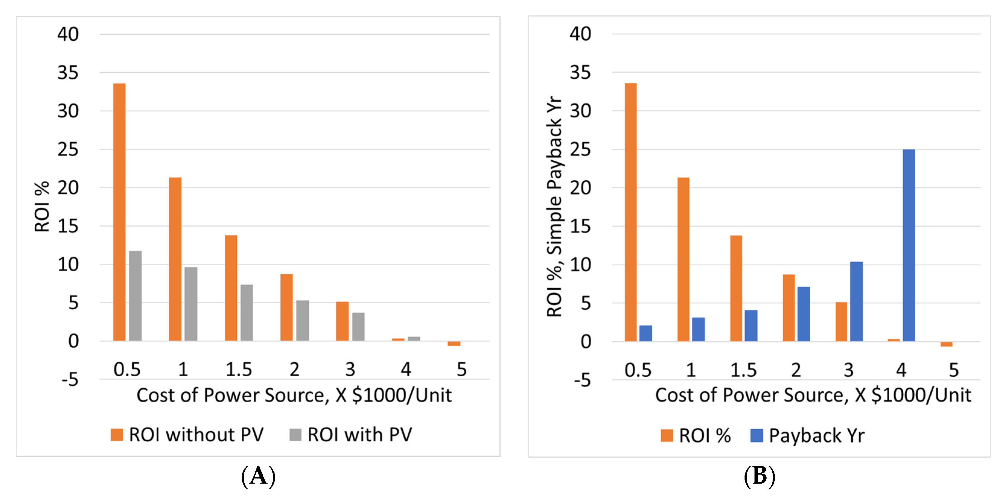
As discussed in the introduction section, the penetration of the cogeneration system into the residential building market is driven by many factors, including environmental and economic (operational expenditure savings) benefits, as discussed above. However, for cogeneration systems to become an effective energy resource in residential buildings, the return on investment (ROI) is critical factor, as noticed in the building equipment and appliance market. The impact of cost of the cogeneration system on ROI and payback was investigated for the 0.4 kW configuration (40% electrical efficiency) with and without PV (0.5 kW) in the target price range of $500 to $5000. The capital expenditure considered included the cost of the cogeneration system, PV ($3.22/Watt, if utilized), as well as the electrical energy storage module ($300/kWh). The mean time to replace/repair the power core was assumed to be 2.5 years of operation, while the cogeneration system design life was considered to be 10 years. The power source did not take into account any tax credits or incentives and no demand response/demand load relief programs were considered in this analysis, reflecting today’s residential tariff structure. Figure 8A displays the ROI of such a system with and without PV. It can be noticed that the high cost of PV lowers the overall ROI compared to the configuration without PV. An ROI of 33% can be achieved with a $500 cogeneration system, which decreases to ~5% if the capital cost of such a system is $3000. Capital costs beyond the $3000 range nullify the operational expenditure savings and do not yield any significant ROI. Figure 8B, on the other hand, shows the simple payback in years for cogeneration system systems without PV. At a target cost of $3000, the payback is ~10 years, while it is only 4 years if the capital cost is $1500.
3.4. Comparison with Heat Pump
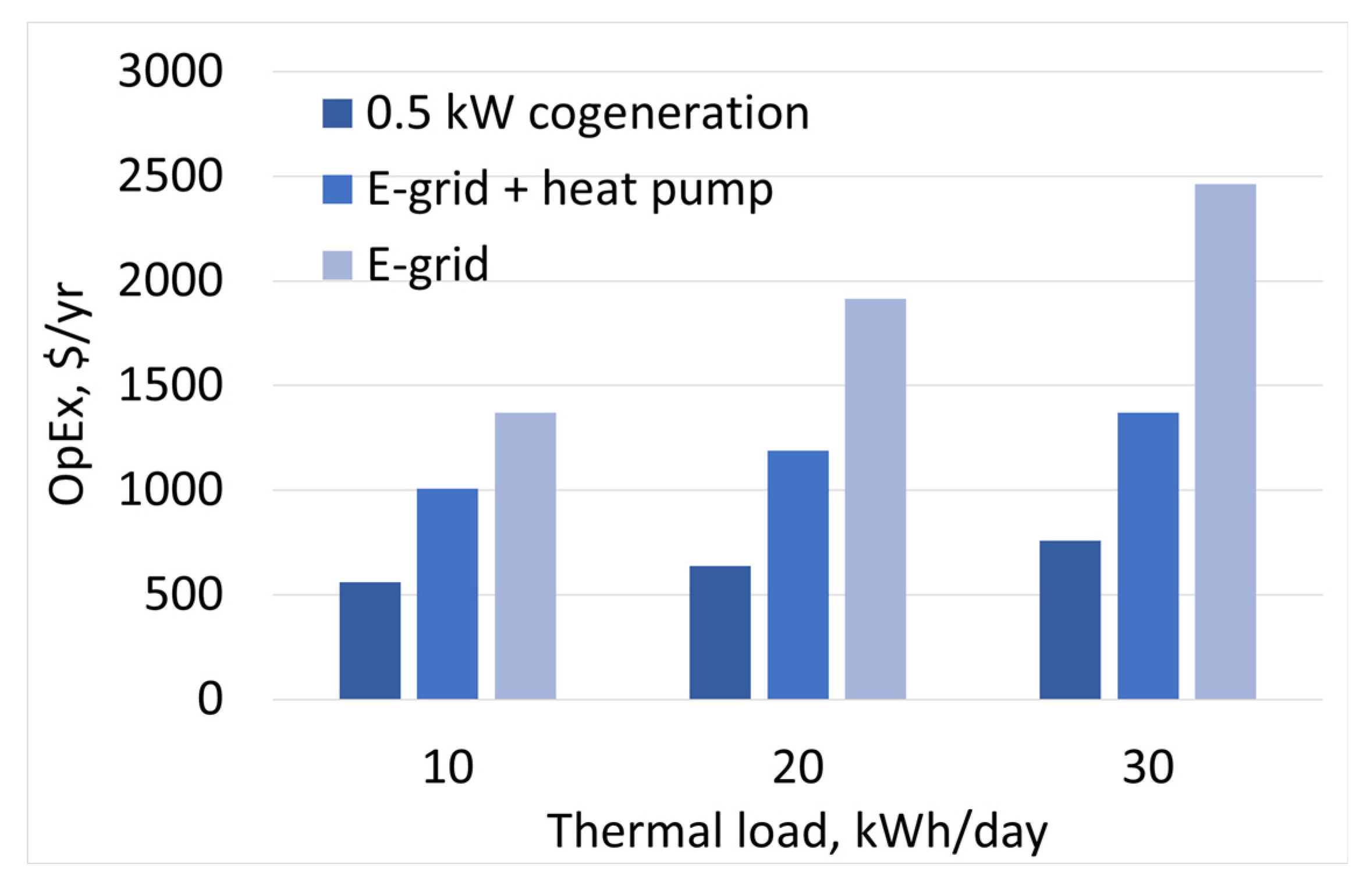
Heat pumps are most efficient in serving the thermal loads of a building. Hence, the performance of a 0.5 kW cogeneration system was compared with that of a heat pump (COP 3.0), and also with a resistive heating system (COP 1.0), both supported by electrical grids with a carbon dioxide factor of 0.63 kg/kWh. The residential building’s average electrical load was assumed to be 15 kWh/day, while the average thermal load was assumed to be 10 kWh/day. The electrical efficiency of the cogeneration system was assumed to be 40%. The analysis presented in Figure 9 and Figure 10 accounts for the complete utilization of the excess thermal energy (via thermal energy storage) produced by the cogeneration system. Figure 9 compares the annual operational expenditure of the three configurations examined. The 0.5 kW cogeneration system is cost effective at all thermal loads considered. The heat pump system is the second most cost-effective solution from an operational economics viewpoint.
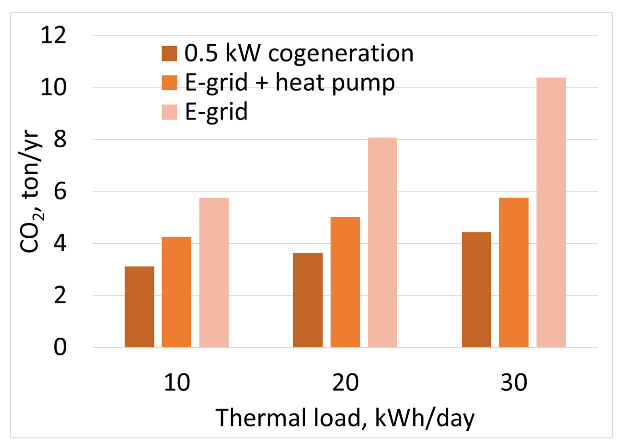
Similarly, Figure 10 compares the annual carbon dioxide emissions from these three configurations. The data presented here accounts for combined emissions associated with electrical grid supply as well as on-site fuel consumption. As shown in the figure, the environmental impact of the cogeneration system is considerably lower compared with the electrical resistance-based heating system; however, compared to the heat pump system, the carbon dioxide reductions are slightly lower for all three thermal loads investigated. For instance, at 20 kWh/day thermal load, the cogeneration system can lower the annual carbon dioxide emissions by ~27% compared to a heat pump system, and by ~55% compared to the electrical heating system with a COP of 1.0.
3.5. Carbon Intensity of E-Grid
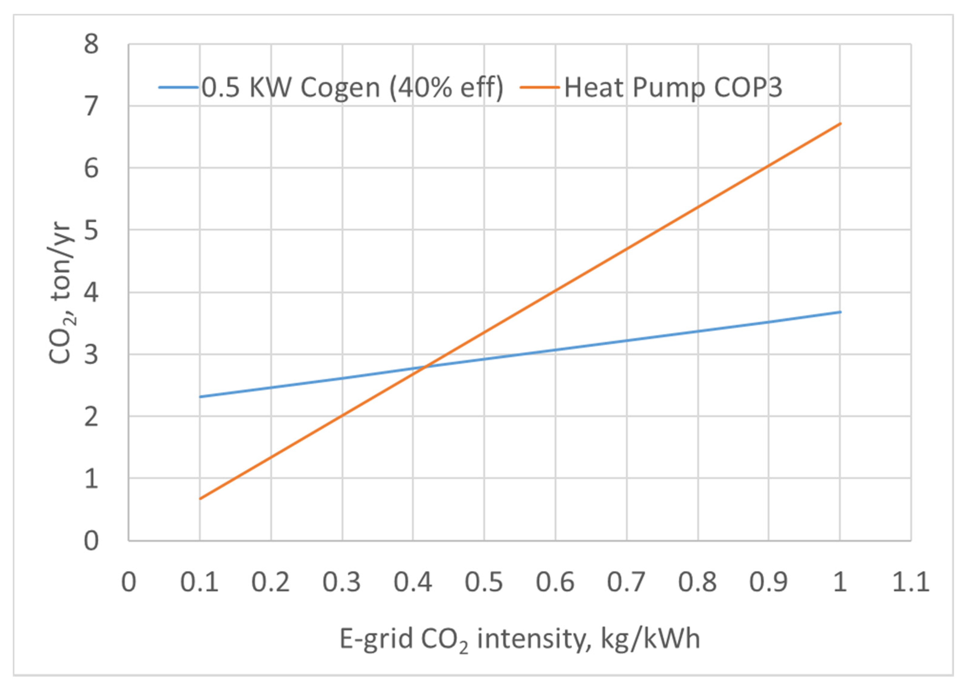
As shown in the above section, the cogeneration system can lower the carbon dioxide emissions compared to electrically driven systems. However, one must consider the carbon intensity of the electrical grid in such analysis. The transformation of the electrical grid with higher contributions from renewable energy sources in the grid infrastructure is continuously lowering the effective carbon intensity of the grid. Hence, the environmental analysis was repeated for different carbon dioxide intensities in the range of 0.1 to 1.0 kg CO2 per kWh of electricity produced by the grid.
Figure 11 compares the annual carbon dioxide footprint of the cogeneration system compared with that of heat pump equipment serving the energy needs of a building consuming an average of 10 kWh/day of thermal energy and 15 kWh/day of electrical energy. As shown in the figure, the 0.5 kW cogeneration system with 40% electrical efficiency loses its environmental benefit if the E-grid’s carbon dioxide intensity falls below 0.4 kg CO2 per kWh electricity.
3.6. Demand Response Incentive
The results presented so far did not consider any demand response incentives; however, the electric tariff structure is transforming and evolving towards meeting the growing global energy needs and such incentives are expected to become commonplace even in residential buildings. Such incentives are also considered to promote better cost allocation among ratepayers, while also helping to reduce strain on the grid. Hence, further studies were conducted to explore the value proposition of a 0.5 kW cogeneration system with an electrical efficiency of 40% in further reducing the operational energy costs in comparison with a heat pump system with COP of 3.0. Demand response (DR) incentive was structured at the rate of $6/kW, optimized according to HOMER®’s demand reduction protocol. Ten DR events were assumed to occur in the summer months of May through September of each year, between 7 a.m. and 7 p.m. Each event duration was assumed to be 4 h long. The operational energy cost savings reached ~50% compared to a heat pump system and >62% compared to electrical heating systems with a COP of 1.0.
4. Conclusions
This study presents a comprehensive analysis of the influence of different system parameters such as power rating, electrical efficiency, unit cost, and power system configuration on energy use, as well as the environmental and economic benefits they offer. The primary objective was to identify the influencing factors which help lower (i) the primary energy consumption, (ii) electrical grid purchases, (iii) annual operational energy cost and (iv) carbon dioxide emissions, without producing excess thermal or electrical energy, but enhancing energy resiliency and efficiency, using a small-scale cogeneration system. This study demonstrates that it is possible to design a small-scale residential building cogeneration system capable of providing environmental and economic benefits without producing excess energy while utilizing < 2kWh of electrical storage capacitance. The practical electrical efficiency of today’s prime mover technologies can lower the carbon footprint of residential buildings even at small scale power output in a baseload configuration while providing operational expenditure savings of >30%. Below are some of the key findings from this study:
- At an electrical grid’s carbon intensity of 0.63 kg/kWh, CO2 emissions can be curtailed by >32% with a 0.1 or 0.2 kW cogeneration system with an electrical efficiency of 25%.
- Cogeneration system sizes of up to 0.6 kW offer higher primary energy efficiency compared to a 30% efficient electrical system, while they decrease to 0.4 kW and 0.2 kW configurations when integrated in a 45% and 60% efficient E-grid network, respectively.
- Operational energy cost savings of 36% to 50% are possible via a cogeneration system (25% electrical efficiency) with a power rating between 0.1 kW and 0.4 kW.
- To be effective as an energy efficient resource in residential buildings, and in order to compete with electrical grid efficiencies > 60%, small scale cogeneration systems (<0.5 kW) must exceed 35% electrical efficiency.
- In a building consuming 15 kWh/day of electrical energy and 10 kWh/day thermal load, a 0.5 kW, 40% electrical efficient cogeneration system can lower the annual carbon dioxide emissions by ~27% compared to a heat pump system (COP of 3.0) and by ~55% compared to the electrical heating system with a COP of 1.0.
- A 0.5 kW cogeneration system with 40% electrical efficiency loses its environmental benefit if the electrical grid’s carbon dioxide intensity falls below 0.4 kg CO2 per kWh electricity.
- Net operating expenditure savings can exceed 60% with a 0.4 kW cogeneration system.
- A 0.4 kW cogeneration system can achieve an ROI of 14% and 8% with a price tag of $1500 and $2000, respectively.
Funding
This research received no external funding.
Acknowledgments
This research was supported by the DOE Office of Energy Efficiency and Renewable Energy (EERE) Building Technologies Office, and used resources at the Building Technologies Research and Integration Center, a DOE-EERE User Facility at Oak Ridge National Laboratory.
Conflicts of Interest
The author declares no conflict of interest.
Nomenclature
| $savings, opex | Operational expenditure savings |
| CO2,grid | Carbon intensity of electrical grid |
| CO2,fuel | Carbon intensity of natural gas combustion |
| COP | Coefficient of performance |
| EES | Electrical energy storage |
| kWh/day | Kilowatt-hours per day |
| kWhsales | Electric sales to grid |
| kWel | Kilowatt, electric |
| kg | Kilogram |
| kWh | Kilowatt-hour |
| m3 | Cubic meters of natural gas |
| MWhgrid/yr | Electrical grid purchases by the building |
| MJ | Megajoules |
| MW | Megawatt |
| MWh | Megawatt-hour |
| PV | Photovoltaic |
| ROI | Return on Investment |
| RTE | Round trip efficiency |
| SOC | Status of charge |
References
- InternationalEnergyAgency. Energy Efficiency: The First Fuel of a Sustainable Global Energy System. 2021. Available online: https://www.iea.org/topics/energy-efficiency (accessed on 27 March 2021).
- Bramstoft, R.; Pizarro-Alonso, A.; Jensen, I.G.; Ravn, H.; Münster, M. Modelling of renewable gas and renewable liquid fuels in future integrated energy systems. Appl. Energy 2020, 268, 114869. [Google Scholar] [CrossRef]
- Sonde, R. Hydrogen: Bridge between renewable energy and fossil fuels. HFC-Hydrogen fuel cells for stationary and mobility applications. Chem. Ind. News 2020, 33, 53–59. [Google Scholar]
- Bessel, V.V.; Koshelev, V.N.; Kutcherov, V.G.; Lopatin, A.S.; Morgunova, M.O. Sustainable transformation of the global energy system: Natural gas in focus. In Proceedings of the IOP Conference Series: Earth and Environmental Science, Ivano-Frankivsk, Ukraine, 21–22 October 2020; IOP Publishing: Bristol, England, 2020. [Google Scholar]
- Islam, M.; Hasanuzzaman, M.; Pandey, A.; Rahim, N. Modern energy conversion technologies. In Energy for Sustainable Development; Elsevier Science & Technology, Academic Press: London, UK, 2020; pp. 19–39. [Google Scholar]
- Amelio, M.; Morrone, P. Residential cogeneration and trigeneration. In Current Trends and Future Developments on (Bio-) Membranes; Elsevier: Amsterdam, the Netherland, 2020; pp. 141–175. [Google Scholar]
- Gandiglio, M.; Ferrero, D.; Lanzini, A.; Santarelli, M. Fuel cell cogeneration for building sector: European status. REHVA J. 2020, 57, 21–25. [Google Scholar]
- Cheekatamarla, P. Performance analysis of hybrid power configurations: Impact on primary energy intensity, carbon dioxide emissions, and life cycle costs. Int. J. Hydrog. Energy 2020, 45, 34089–34098. [Google Scholar] [CrossRef]
- Colmenares-Quintero, R.F.; Latorre-Noguera, L.-F.; Colmenares-Quintero, J.-F.; Dibdiakova, J. Techno-environmental assessment of a micro-cogeneration system based on natural gas for residential application. CT&F-Cienc. Tecnol. Futuro 2018, 8, 101–112. [Google Scholar]
- Longo, S.; Cellura, M.; Guarino, F.; Brunaccini, G.; Ferraro, M. Life cycle energy and environmental impacts of a solid oxide fuel cell micro-CHP system for residential application. Sci. Total Environ. 2019, 685, 59–73. [Google Scholar] [CrossRef] [PubMed]
- Mahian, O.; Javidmehr, M.; Kasaeian, A.; Mohasseb, S.; Panahi, M. Optimal sizing and performance assessment of a hybrid combined heat and power system with energy storage for residential buildings. Energy Convers. Manag. 2020, 211, 112751. [Google Scholar] [CrossRef]
- Fazelpour, F.; Farahi, S.; Soltani, N. Techno-economic analysis of hybrid power systems for a residential building in Zabol, Iran. In Proceedings of the 2016 IEEE 16th International Conference on Environment and Electrical Engineering (EEEIC), Florence, Italy, 7–10 June 2016; IEEE: New York, NY, USA, 2016. [Google Scholar]
- Carlucci, A.P.; De Monte, V.; De Risi, A.; Strafella, L. Benefits of Enabling Technologies for the ICE and Sharing Strategies in a CHP System for Residential Applications. J. Energy Eng. 2017, 143, 04017007. [Google Scholar] [CrossRef]
- de Santoli, L.; Basso, G.L.; Albo, A.; Bruschi, D.; Nastasi, B. Single cylinder internal combustion engine fuelled with H2NG operating as micro-CHP for residential use: Preliminary experimental analysis on energy performances and numerical simulations for LCOE assessment. Energy Procedia 2015, 81, 1077–1089. [Google Scholar] [CrossRef] [Green Version]
- Atănăsoae, P. Technical and economic assessment of micro-cogeneration systems for residential applications. Sustainability 2020, 12, 1074. [Google Scholar] [CrossRef] [Green Version]
- Ferreira, A.C.M.; Teixeira, S.F.C.F.; Silva, R.G.; Silva Ângela, M. Thermal-economic optimisation of a CHP gas turbine system by applying a fit-problem genetic algorithm. Int. J. Sustain. Energy 2018, 37, 354–377. [Google Scholar] [CrossRef]
- Kim, C.K.; Yoon, J.Y. Performance analysis of bladeless jet propulsion micro-steam turbine for micro-CHP (combined heat and power) systems utilizing low-grade heat sources. Energy 2016, 101, 411–420. [Google Scholar] [CrossRef]
- Ellamla, H.R.; Staffell, I.; Bujlo, P.; Pollet, B.G.; Pasupathi, S. Current status of fuel cell based combined heat and power systems for residential sector. J. Power Sources 2015, 293, 312–328. [Google Scholar] [CrossRef]
- Bizon, N.; Mazare, A.G.; Ionescu, L.M.; Enescu, F.M. Optimization of the proton exchange membrane fuel cell hybrid power system for residential buildings. Energy Convers. Manag. 2018, 163, 22–37. [Google Scholar] [CrossRef]
- Sorace, M.; Gandiglio, M.; Santarelli, M. Modeling and techno-economic analysis of the integration of a FC-based micro-CHP system for residential application with a heat pump. Energy 2017, 120, 262–275. [Google Scholar] [CrossRef]
- Hormaza-Mejia, A.; Zhao, L.; Brouwer, J. SOFC Micro-CHP system with thermal energy storage in residential applications. In Proceedings of the International Conference on Fuel Cell Science, Engineering and Technology, Charlotte, NC, USA, 26–30 June 2017; American Society of Mechanical Engineers: New York, NY, USA, 2017. [Google Scholar]
- Adam, A.; Fraga, E.S.; Brett, D.J. A modelling study for the integration of a PEMFC micro-CHP in domestic building services design. Appl. Energy 2018, 225, 85–97. [Google Scholar] [CrossRef]
- Ito, H. Economic and environmental assessment of residential micro combined heat and power system application in Japan. Int. J. Hydrog. Energy 2016, 41, 15111–15123. [Google Scholar] [CrossRef]
- Yang, F.; Huang, N.; Sun, Q.; Cheng, L.; Wennersten, R. Modeling and techno-economic analysis of the heat pump-integrated PEMFC-based micro-CHP system. Energy Procedia 2018, 152, 83–88. [Google Scholar] [CrossRef]
- Baniasadi, E.; Toghyani, S.; Afshari, E. Exergetic and exergoeconomic evaluation of a trigeneration system based on natural gas-PEM fuel cell. Int. J. Hydrog. Energy 2017, 42, 5327–5339. [Google Scholar] [CrossRef]
- Wang, Y.; Shi, Y.; Cai, N.; Wang, Y. Dynamic analysis of a micro CHP system based on flame fuel cells. Energy Convers. Manag. 2018, 163, 268–277. [Google Scholar] [CrossRef]
- Chen, W.-L.; Huang, C.-W.; Li, Y.-H.; Kao, C.-C.; Cong, H.T. Biosyngas-fueled platinum reactor applied in micro combined heat and power system with a thermophotovoltaic array and stirling engine. Energy 2020, 194, 116862. [Google Scholar] [CrossRef]
- Qiu, K.; Hayden, A. Implementation of a TPV integrated boiler for micro-CHP in residential buildings. Appl. Energy 2014, 134, 143–149. [Google Scholar] [CrossRef]
- Zhang, Y.; Wang, X.; Cleary, M.; Schoensee, L.; Kempf, N.; Richardson, J. High-performance nanostructured thermoelectric generators for micro combined heat and power systems. Appl. Therm. Eng. 2016, 96, 83–87. [Google Scholar] [CrossRef] [Green Version]
- Olawole, O.C.; De, D.; Oyedepo, S.O.; Olawole, O.F.; Joel, E.S. Current status of thermionic conversion of solar energy. Curr. Sci. 2020, 118, 543. [Google Scholar]
- Qiu, K.; Entchev, E. Development of an organic Rankine cycle-based micro combined heat and power system for residential applications. Appl. Energy 2020, 275, 115335. [Google Scholar] [CrossRef]
- Calise, F.; Cappiello, F.L.; D’Accadia, M.D.; Vicidomini, M. Energy and economic analysis of a small hybrid solar-geothermal trigeneration system: A dynamic approach. Energy 2020, 208, 118295. [Google Scholar] [CrossRef]
- Calise, F.; Cappiello, F.L.; D’Accadia, M.D.; Vicidomini, M. Thermo-economic analysis of hybrid solar-geothermal polygeneration plants in different configurations. Energies 2020, 13, 2391. [Google Scholar] [CrossRef]
- Abu-Heiba, A.; Gluesenkamp, K.R.; LaClair, T.J.; Cheekatamarla, P.; Munk, J.D.; Thomas, J.; Boudreaux, P.R. Analysis of power conversion technology options for a self-powered furnace. Appl. Therm. Eng. 2021, 188, 116627. [Google Scholar] [CrossRef]
- Cheekatamarla, P.; Abu-Heiba, A. A Comprehensive Review and Qualitative Analysis of Micro-Combined Heat and Power Modeling Approaches. Energies 2020, 13, 3581. [Google Scholar] [CrossRef]
- Dorer, V.; Weber, A. Energy and CO2 emissions performance assessment of residential micro-cogeneration systems with dynamic whole-building simulation programs. Energy Convers. Manag. 2009, 50, 648–657. [Google Scholar] [CrossRef]
- Roselli, C.; Marrasso, E.; Tariello, F.; Sasso, M. How different power grid efficiency scenarios affect the energy and environmental feasibility of a polygeneration system. Energy 2020, 201, 117576. [Google Scholar] [CrossRef]
- Marrasso, E.; Roselli, C.; Sasso, M.; Tariello, F. Comparison of centralized and decentralized air-conditioning systems for a multi-storey/multi users building integrated with electric and diesel vehicles and considering the evolution of the national energy system. Energy 2019, 177, 319–333. [Google Scholar] [CrossRef]
- Muresan, C.; Djama, K.; Robinet, P.; Sato, T. Internal combustion engine micro-chp system dedicated to residential market result and experiences from an existing French individual house field test. In Proceedings of the International Gas Research Conference 2017, Rio de Janeiro, Brazil, 24–26 May 2017; pp. 1302–1309. [Google Scholar]
- Yaïci, W.; Entchev, E.; Longo, M. Performance Analysis of Regenerative Organic Rankine Cycle System for Solar Micro Combined Heat and Power Generation Applications. In Proceedings of the 2018 7th International Conference on Renewable Energy Research and Applications (ICRERA), Ankara, Turkey, 26–29 September 2018; IEEE: New York, NY, USA, 2018. [Google Scholar]
- EIA. How Much Energy is Consumed in U.S. Buildings? 2020. Available online: https://www.eia.gov/tools/faqs/faq.php?id=86&t=1#:~:text=Energy%20consumption%20by%20the%20U.S.,British%20thermal%20units%20(Btu) (accessed on 29 June 2020).
- Masters, G.M. Renewable and Efficient Electric Power Systems; John Wiley & Sons: Hoboken, NJ, USA, 2013. [Google Scholar]
- Table HC6.6 Space Heating in U.S. Homes by Climate Region. 2020. Available online: https://www.eia.gov/consumption/residential/data/2015/hc/php/hc6.6.php (accessed on 29 June 2020).
- Energy, H. HOMER pro. HOMER Energy; Homer by UL: Boulder, CO, USA, 2018. [Google Scholar]
- Lambert, T.; Gilman, P.; Lilienthal, P. Micropower System Modeling with Homer. In Integration of Alternative Sources of Energy; National Renewable Energy Lab: Golden, CO, USA, 2006; pp. 379–418. [Google Scholar]
- Kansara, B.U.; Parekh, B.R. Modelling and simulation of distributed generation system using HOMER software. In Proceedings of the 2011 International Conference on Recent Advancements in Electrical, Electronics and Control Engineering, IConRAEeCE’11—Proceedings, Sivakasi, India, 15–17 December 2011. [Google Scholar]
- How Much Electricity Does an American Home Use? 2020. Available online: https://www.eia.gov/tools/faqs/faq.php?id=97&t=3 (accessed on 25 August 2020).
- EIA. Commercial Buildings Energy Consumption Survey (CBECS). 2020. Available online: https://www.eia.gov/consumption/commercial/data/2012/c&e/cfm/pba4.php (accessed on 25 August 2020).
- Al Moussawi, H.; Fardoun, F.; Louahlia, H. Selection based on differences between cogeneration and trigeneration in various prime mover technologies. Renew. Sustain. Energy Rev. 2017, 74, 491–511. [Google Scholar] [CrossRef]
- Open Energy Database. Open Data @ DOE. 2020. Available online: https://www.energy.gov/data/open-energy-data (accessed on 27 September 2020).
- New Energy, Clear Savings. Transparent Costs, Accurate Forecasts, Measured Savings. Available online: https://www.genability.com/ (accessed on 25 April 2020).
- NASA. Prediction of Worlwide Energy Resources. Available online: https://power.larc.nasa.gov/ (accessed on 15 March 2020).
- NREL, U.S. DOE. National Solar Radiation Database. Available online: https://nsrdb.nrel.gov/ (accessed on 15 March 2020).
- Ralon, P.; Taylor, M.; Ilas, A.; Diaz-Bone, H.; Kairies, K. Electricity storage and renewables: Costs and markets to 2030. In Proceedings of the International Renewable Energy Agency, Abu Dhabi, United Arab Emirates, 15 January 2017; p. 164. [Google Scholar]
- EIA. Today in Energy 2021. Available online: https://www.eia.gov/todayinenergy/detail.php?id=46756#:~:text=According%20to%20data%20from%20the,%2Dtrip%20efficiency%20of%2079%25 (accessed on 19 April 2020).
- Goldie-Scot, L. A behind the scenes take on lithium-ion battery prices. In Bloomberg New Energy Finance; Bloomberg: London, UK, 2019; p. 5. [Google Scholar]
- EIA. Electric Power Monthly. 2021. Available online: https://www.eia.gov/electricity/monthly/epm_table_grapher.php?t=epmt_5_6_a (accessed on 19 April 2020).
- EIA. Selected National Average Natural Gas Prices, 2016–2021. Available online: https://www.eia.gov/naturalgas/monthly/pdf/table_03.pdf (accessed on 15 March 2021).
- EIA. How Much Carbon Dioxide is Produced per Kilowatthour of U.S. Electricity Generation. 2021. Available online: https://www.eia.gov/tools/faqs/faq.php?id=74&t=11 (accessed on 17 March 2021).
- EIA. How Much Electricity Does an American Home Use? 2021. Available online: https://www.eia.gov/tools/faqs/faq.php?id=97&t=3 (accessed on 1 April 2021).
- Groll, E.A.; Baxter, V.D. IEA HPT ANNEX 41–Cold Climate Heat Pumps: US Country Report. 2017; Oak Ridge National Lab (ORNL): Oak Ridge, TN, USA, 2017.
- U.S.DOE. Fuel Properties Comparison. 2021. Available online: https://afdc.energy.gov/files/u/publication/fuel_comparison_chart.pdf (accessed on 15 March 2021).
- Electric Power Annual Report 2019; Energy Information Agency: Washington, DC, USA, 2021.
- A Comparison of Energy Usage, Operating Costs, and Carbon DIOXIDE Emissions of Home Appliances; American Gas Association: Washington, DC, USA, 2017.
- OPENEI. Commercial and Residential Hourly Load Profiles for all TMY3 Locations in the United States. 2021. Available online: https://openei.org/datasets/files/961/pub/RESIDENTIAL_LOAD_DATA_E_PLUS_OUTPUT/BASE/ (accessed on 15 February 2021).
- How Much Carbon Dioxide Is Produced per Kilowatthour of U.S. Electricity Generation? 2020. Available online: https://www.eia.gov/tools/faqs/faq.php?id=74&t=11 (accessed on 9 July 2020).
- Source Energy, Energystar Portfolio Manager. 2019. Available online: https://portfoliomanager.energystar.gov/pdf/reference/Source%20Energy.pdf (accessed on 9 July 2020).
Figure 1.
Generic residential building energy consumption profile considered for the analysis: (A) time of the day and (B) day of the year demand.
Figure 1.
Generic residential building energy consumption profile considered for the analysis: (A) time of the day and (B) day of the year demand.

Figure 2.
Generic hybrid energy system configuration utilized in this study.

Figure 3.
Influence of generator power scale on E-Grid demand, total carbon dioxide emissions, excess electrical and thermal energy produced, and net combined efficiency of the residential energy system. (A) CO2, E-Grid purchases vs. different configurations. (B) Total energy efficiency vs. cogeneration system power rating. No PV or thermal energy storage in the cogeneration system configuration.

Figure 4.
Impact of energy source configuration on carbon dioxide emissions, operational expenditure, primary energy consumption, heating fuel demand. (A) Reduction in CO2 and operational expenses. (B) Total primary energy and additional heating fuel consumption. No PV in the cogeneration system configuration.

Figure 5.
Energy performance analysis of cogeneration system-based configurations with different prime power electrical efficiencies. Combined load of 28 kWh/day, 0.5 kW PV, 0.4 kW PM, and 2 kWh electrical storage capacitance.
Figure 5.
Energy performance analysis of cogeneration system-based configurations with different prime power electrical efficiencies. Combined load of 28 kWh/day, 0.5 kW PV, 0.4 kW PM, and 2 kWh electrical storage capacitance.

Figure 6.
Combined energy efficiency of cogeneration system-based configurations with different prime power electrical efficiencies. Combined load of 28 kWh/day, 0.5 kW PV, 0.4 kW PM, and 2 kWh electrical storage capacitance.
Figure 6.
Combined energy efficiency of cogeneration system-based configurations with different prime power electrical efficiencies. Combined load of 28 kWh/day, 0.5 kW PV, 0.4 kW PM, and 2 kWh electrical storage capacitance.

Figure 7.
Environmental and economic analysis of cogeneration system-based configurations with different electrical efficiencies. Combined load of 28 kWh/day, 0.5 kW PV, 0.4 kW PM, and 2 kWh electrical storage capacitance.
Figure 7.
Environmental and economic analysis of cogeneration system-based configurations with different electrical efficiencies. Combined load of 28 kWh/day, 0.5 kW PV, 0.4 kW PM, and 2 kWh electrical storage capacitance.

Figure 8.
Economic analysis of the cogeneration system. (A) Influence of cost on ROI, with and without PV. (B) Payback period at different cogeneration system costs (no PV).
Figure 8.
Economic analysis of the cogeneration system. (A) Influence of cost on ROI, with and without PV. (B) Payback period at different cogeneration system costs (no PV).

Figure 9.
Annual operational expenditure of different system configurations with variable thermal loads: 0.5 kW cogeneration system at 40% electrical efficiency (2 kWh EES), heat pump with COP 3.0, and baseline electrical grid supported heating system (COP = 1.0); 15 kWh/day of electrical load, no PV.

Figure 10.
Annual carbon dioxide emissions of different system configurations with variable thermal loads: 0.5 kW cogeneration system at 40% electrical efficiency (2 kWh EES), heat pump with COP 3.0, and baseline electrical grid supported heating system (COP = 1.0); 15 kWh/day of electrical load, no PV.

Figure 11.
Annual carbon dioxide emissions of a residential building served by a 0.5 kW cogeneration system (40% electrical efficiency) or E-grid-supported heat pump system (COP-3).
Figure 11.
Annual carbon dioxide emissions of a residential building served by a 0.5 kW cogeneration system (40% electrical efficiency) or E-grid-supported heat pump system (COP-3).


Table 1.
Simulation model’s components and their primary operating parameters and constraints.
| Simulation Model Component | Parameter/Variable | Notes |
|---|---|---|
| Utility/Tariff | Consumption, demand, and fixed charges or simple tariff with user-defined cost of electricity | $/kWh or tariff database from Genability |
| Utility/Tariff | Grid sale limit | kW |
| Utility/Tariff | Emissions factors | CO2, CO, SO2, NOx, Hydrocarbons, particulate matter in g/kWh |
| Electric load/Thermal load | Time-series file | From Open EI database or user-defined synthetic load profile |
| PM | Fuel type and value | Natural gas, propane, diesel, biodiesel, ethanol, methanol etc. |
| PM | Fixed generator capacity | Capacity in kW |
| PM | Fuel curve | Fuel units/hr/kW |
| PM | Minimum allowable load on the generator | 0–100% |
| PM | Heat recovery ratio | Recoverable thermal energy, 0–100% |
| PM | Lifetime | Hours of operation |
| PM | Schedule | PM on/off/optimized selection feature during time of the day and day of the year |
| Energy storage | Idealized battery | Idealized model—nominal voltage, capacity (kWh), round trip efficiency (%), maximum charge/discharge current (A), cost ($/module), throughput lifetime (kWh), initial state of charge (%), minimum state of charge (%). |
| Boiler | Efficiency | % along with user selectable fuel and cost |
| Photovoltaic | Cost, derating factor | $/kW, 0–100% |
| Photovoltaic | Solar GHI resource or time series file | kWh/m2 |
Table 2.
Performance and cost modeling assumptions.
| Parameter | Value |
|---|---|
| Discount Rate | 8% |
| Inflation Rate | 2% |
| Project Lifetime | 20 Years |
| Day-to-Day Load Variability | 10%, random |
| Time step | 20 min |
| Utility Tariff, Effective Date | 1/1/2021 |
| Generic flat plate PV cost [54] | $3.22/watt |
| Electrical energy storage’s (EES) round trip efficiency (RTE) [55] | 80% |
| EES Status of Charge, SOCmin | 20% |
| Initial SOC of EES | 100% |
| Capital cost of EES [56] | $300/kWh |
| Energy charges, $grid [57] | $0.15/kWh |
| Energy sold to grid, $grid sales | $0.1/kWh |
| Cost of natural gas, $fuel [58] | $0.3/m3 |
| Incentive, Investment Tax Credit (PV only) | 30% of capital cost (100% CapEx eligible) |
| Incentive, Bonus depreciation (PV only) | 50% in first year, marginal tax rate of 21% |
| Demand Response | $6/kW, 9 random events/yr, 4 hrs/event |
| Carbon intensity of electrical grid, CO2,grid [59] | 0.1–1.0 kg/kWh |
| Carbon intensity of natural gas, CO2,fuel | 1.95 kg/m3 |
| Power generator rating [49] | 0.1–1 kW |
| Daily building electrical load [47,60] | 15 kWh |
| Daily building thermal load | 10–30 kWh |
| Electrical efficiency of the power generator [49] | 25–50% |
| Thermal recovery efficiency | 75% |
| Heat Pump COP, average [61] | 3.0 |
| Electrical heating equipment COP | 1.0 |
| EES capacity | 2 kWh |
| Energy density of natural gas fuel [62] | 53.6 MJ/kg |
| Electrical Grid efficiency [63] | 30–60% |
| Natural gas site delivery efficiency [64] | 92% |
| Mean time to replace/repair (MTTR) the power generator | 2.5 years or 22,000 h of operation |
| Salvageable value of the power generator | 25% of the initial cost |
Publisher’s Note: MDPI stays neutral with regard to jurisdictional claims in published maps and institutional affiliations. |
© 2021 by the author. Licensee MDPI, Basel, Switzerland. This article is an open access article distributed under the terms and conditions of the Creative Commons Attribution (CC BY) license (https://creativecommons.org/licenses/by/4.0/).
Share and Cite
MDPI and ACS Style
Cheekatamarla, P.K. Decarbonization of Residential Building Energy Supply: Impact of Cogeneration System Performance on Energy, Environment, and Economics. Energies 2021, 14, 2538. https://0-doi-org.brum.beds.ac.uk/10.3390/en14092538
AMA Style
Cheekatamarla PK. Decarbonization of Residential Building Energy Supply: Impact of Cogeneration System Performance on Energy, Environment, and Economics. Energies. 2021; 14(9):2538. https://0-doi-org.brum.beds.ac.uk/10.3390/en14092538
Chicago/Turabian StyleCheekatamarla, Praveen K. 2021. "Decarbonization of Residential Building Energy Supply: Impact of Cogeneration System Performance on Energy, Environment, and Economics" Energies 14, no. 9: 2538. https://0-doi-org.brum.beds.ac.uk/10.3390/en14092538
Note that from the first issue of 2016, this journal uses article numbers instead of page numbers. See further details here.