
Adaptive Driving Cycles of EVs for Reducing Energy Consumption
by
 , , , and
Iwona Komorska
1,* ,
,
Andrzej Puchalski
1,
Andrzej Niewczas
2,
Marcin Ślęzak
2 and
Tomasz Szczepański
2 1
Department of Mechanical Engineering, Kazimierz Pulaski University of Technology and Humanities in Radom, Malczewskiego 29, 26-600 Radom, Poland
2
Motor Transport Institute, Jagiellońska 80, 03-301 Warszawa, Poland
*
Author to whom correspondence should be addressed.
Energies 2021, 14(9), 2592; https://0-doi-org.brum.beds.ac.uk/10.3390/en14092592
Submission received: 22 March 2021
/
Revised: 16 April 2021
/
Accepted: 27 April 2021
/
Published: 1 May 2021
(This article belongs to the Special Issue Electrified Powertrains for a Sustainable Mobility: Topologies, Design and Integrated Energy Management Strategies)
Abstract
:A driving cycle is a time series of a vehicle’s speed, reflecting its movement in real road conditions. In addition to certification and comparative research, driving cycles are used in the virtual design of drive systems and embedded control algorithms, traffic management and intelligent road transport (traffic engineering). This study aimed to develop an adaptive driving cycle for a known route to optimize the energy consumption of an electric vehicle and improve the driving range. A novel distance-based adaptive driving cycle method was developed. The proposed algorithm uses the segmentation and iterative synthesis procedures of Markov chains. Energy consumption during driving is monitored on an ongoing basis using Gaussian process regression, and speed and acceleration are corrected adaptively to maintain the planned energy consumption. This paper presents the results of studies of simulated driving cycles and the performance of the algorithm when applied to the real recorded driving cycles of an electric vehicle.
1. Introduction
The popularization of electric vehicles may decrease air pollution, particularly in cities. The more fossil-fuel-burning vehicles are replaced with electric vehicles, the less harmful substances (pollutants in particulate matter and gases, mainly nitrogen oxides and sulfur oxides) are released into the air. This is the most significant benefit of electromobility from the perspective of environmental impact. It will also reduce the emissions of greenhouse gases (particularly carbon dioxide and ozone). For vehicle owners, the primary advantage is significantly lower operating costs compared to those of conventional vehicles. An energy management system is critical for the development of electric vehicles because it directly affects their capacity to save energy. Power management aims to create the optimum policy for controlling power supplied to the vehicle. The applied driving cycle is required to optimize and assess power management in electric vehicles.
Predicting the driving cycle of a vehicle is becoming increasingly important in modern intelligent transport, particularly for controlling energy consumption in electric vehicles, planning the trajectory of autonomous terrestrial vehicles, energy management in hybrid electric vehicles, etc. In general, driving cycles illustrate changes in vehicle speed as a function of time. They are of fundamental importance to vehicle engineering. Originally, the primary application of driving cycles was to identify the performance characteristics of a vehicle, such as exhaust emissions and fuel consumption for cars with an internal combustion engine. Along with the development of HEVs, PHEVs and EVs, many studies have addressed the adaptation of driving cycles to these types of vehicles [1,2,3,4,5,6].
Driving cycles should reflect actual road conditions as well as local conditions in a particular country or region. Driving cycles with equivalent properties can be generated only using a dataset with recorded information about a vehicle or fleet operation as the basis for generating time signals and final assessment of the quality of induced cycles. Many properties of the driving profile characterizing local driving cycles, such as the average, maximum and minimum values and standard deviations of speed, acceleration and delay, have been defined in the listed articles [1,3,7,8,9,10,11,12]. The impact of the velocity profile on energy consumption in EVs is analyzed in [13].
There are various methods for generating driving cycles, and they are still being developed. In general, however, three primary approaches can be identified: segmentation, Markov chain method and mixed method (a combination of the first two methods). Each method requires a sufficiently large dataset. The cycle is divided into microtrips in the segmentation method, defined as the speed trace between two successive stops [10] or as sections of the route grouped according to specific criteria, such as different road types, traffic conditions or speed limits. Segments are combined stochastically to generate new driving cycles.
The Markov chain method represents another mathematical approach to driving cycle generation. In the simplest algorithm, speeds are divided into classes, and the probability of transition from class to class is included in the TPM. Then, the TPM and speed probability distribution are used to generate new driving cycles. Their equivalence to the reference cycle is verified based on specific criteria [14,15,16,17,18,19,20,21,22,23].
The mixed method combines the two methods mentioned above so that the segment classes (e.g., cruising, idling, acceleration, deceleration or other defined classes) are selected according to the Markov chain algorithm [1,6,24,25]. The methods used for generating driving cycles in this study are discussed more specifically in Section 2.
Previous studies on driving cycles were used to synthesize the type of drive and the city region’s test cycle characteristic. The new approach proposed in this article consists of modifying the driving cycle during its duration to the driving range extension based on well-known Markov process models. Here, energy consumption is estimated based on a statistical model (machine learning method), which is easily determined for each vehicle based on an exemplary driving profile. We go a step further by proposing a modification of the velocity profile during its duration using the new DBADC (distance-based adaptive driving cycle) method. The purpose of this study is to predict the driving cycle and correct it on an ongoing basis depending on road conditions and the vehicle energy consumption. Because of this purpose, driving cycles will be considered as distance-based velocity and not as time-based velocity, as is usually the case. The transition probability matrix (TPM) will be corrected on an ongoing basis during driving, not exceeding the energy-use boundary of a particular route. This method is dedicated to electric vehicles with autopilot feature and driven on specific routes, such as cars rented for a short time in the form of car-sharing and delivery vehicles, buses, etc.
2. Methods
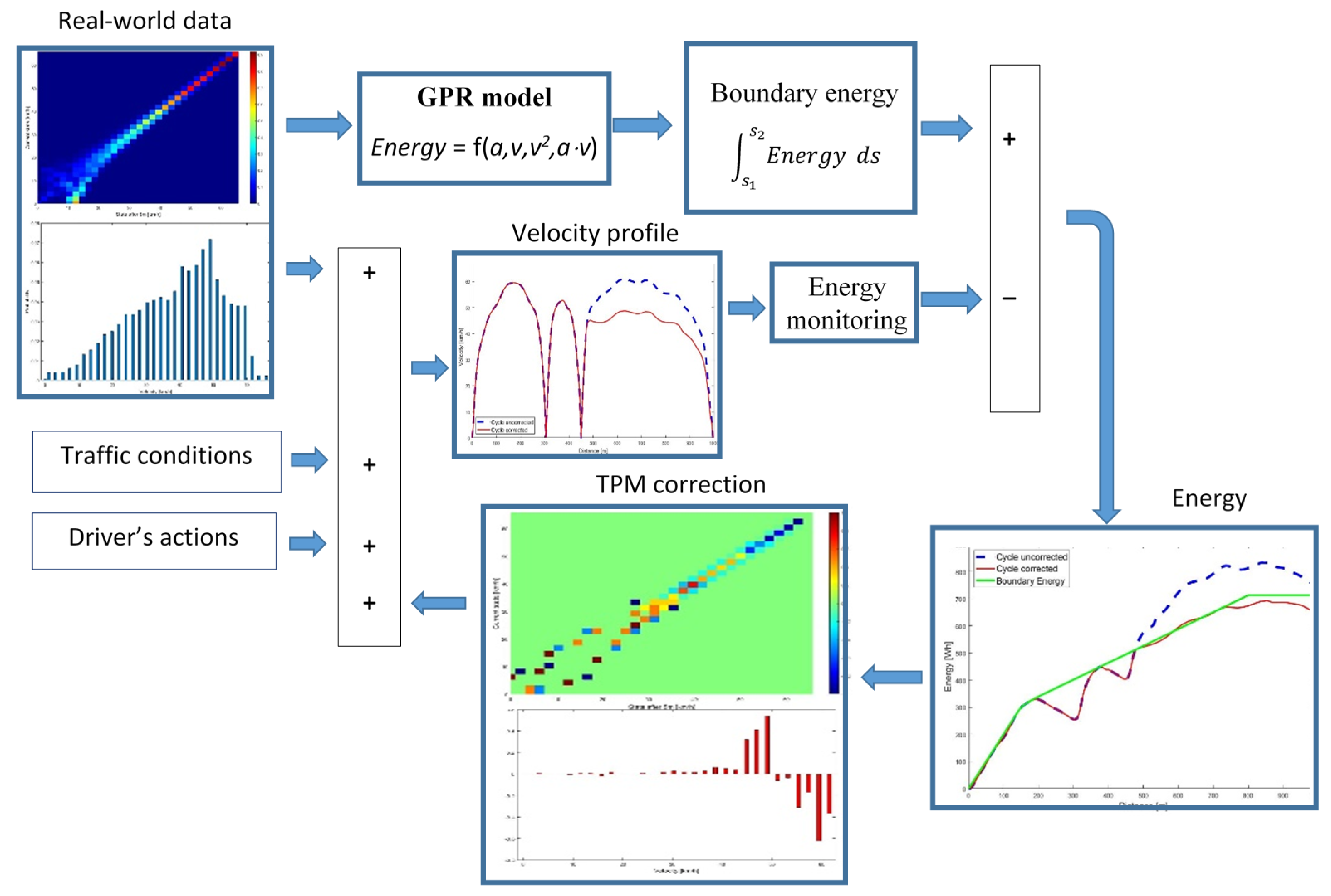
This study uses the segmentation method and iterative Markov chains. Figure 1 shows an illustration of the method, referred to as distance-based adaptive driving cycle (DBADC), which consists of the following components: data collection and their synchronization based on distance, route segmentation and determination of the TPM for the segments, generation of a representative driving cycle and estimated energy consumption using Gaussian process regression (GPR; model-based energy calculation), and on-line correction of the current cycle (an adaptation of the current driving cycle).
First, it is necessary to collect a dataset of driving cycles on routes in the particular region or on planned routes and associated instantaneous or average electricity consumption during these driving cycles.
2.1. Cycle Segmentation
A typical microtrip in a driving cycle is presented by Austin et al. [26] as the speed trace between two stops. The cycle begins with the idling phase, followed by the acceleration, cruise and deceleration phases. The entire driving cycle consists of such microtrips. The duration of the driving cycle varies depending on average speed and acceleration. Austin et al. suggest three methods for combining microtrips: random, best incremental (based on the Watson plot) and hybrid. The set of driving cycle candidates thus generated is used to select the driving cycle for which the probability distribution of acceleration and speed most closely resembles the actual driving dataset. Further versions of this method are based on improved methods for stochastically combining microtrips. Determination of the optimum combination of microtrips using a genetic algorithm (GA) is proposed in [10]. In this, segments with differing numbers of microtrips are combined until the desired driving cycle duration is reached. In [27], Nesamani et al. used microtrips based on road type to develop a driving cycle for PHEV city buses. A computer program was devised to select microtrips at random until the target distance was reached. The percentage of microtrips depending on road type and time spent on every road type was also calculated to further represent the observed data. In [6], kinematic segments were divided depending on the distance between successive bus stops, whereas the two-dimensional Monte Carlo Markov chain (MCMC) method was used to synthesize driving cycles between each interval of subsequent bus stops.
In the segmentation method, real driving cycles are divided into driving segments grouped according to similar average speed, road surface, traffic conditions or other criteria. The segments are connected stochastically. Lin and Niemeier [24] used the acceleration signal and the maximum likelihood estimation (MLE) method to divide the cycle into segments to associate the segment with specific modal operating conditions (e.g., cruise control, idling, acceleration or deceleration). Here, every class characterizes the driving style and, consequently, also represents a possible state in the Markov chain. Zähringer et al. [28] present the enhanced modal cycle construction (EMCC) method, which is a modification of the method described in [24]. Here, the global driving state acceleration, deceleration and cruising are subdivided into substates. This enables development of a complete driving cycle using a first-order Markov chain with a constant transition matrix. The control segments to be combined are constructed parametrically based on characteristic values.
This paper proposes dividing a route into segments. Depending on the type of vehicle, segments range from one to several microtrips, which do not have to begin or end with the idling phase. For instance, for cars or delivery vehicles, the segment may include the route between intersections or longer, even though the idling phase may be absent when passing through an intersection. For a bus, the segments may include the route from one stop to another, with traffic lights on the way and a segment beginning and ending with the idling phase.
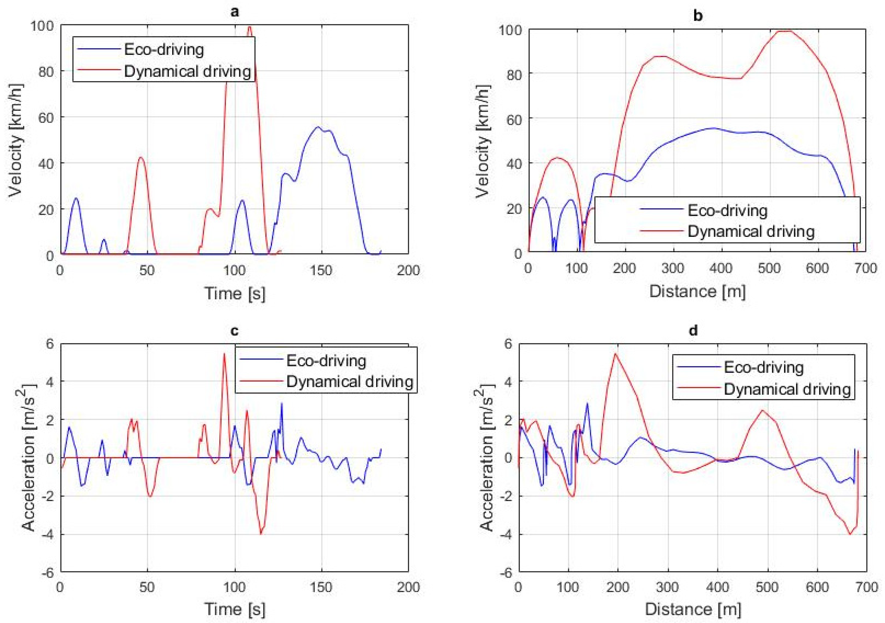
Figure 2 shows a sample segment of a driving cycle, recorded between traffic lights and covering a distance of approximately 700 m, frequently driven in heavy, congested traffic.
The two sample segments between traffic lights shown in Figure 2 have different maximum speeds, accelerations and travel times. This makes it difficult to compare them in the time domain (Figure 2a,c). However, cycles analyzed in the distance domain (Figure 2b,d) are more transparent. Because driving cycles are recorded at equal time intervals, it is necessary to use a cycle synchronization procedure based on travel distance.
The length of the segment is selected individually depending on the route and the type of vehicle. A single microtrip between traffic lights is shown in Figure 2. However, the segments should contain more microtrips, grouped according to road conditions such as driving on the ring road, route with heavy traffic (city center) and a built-up zone (residential). This allows for more effective cycle correction.
When the segments are analyzed in the distance domain, the idling phase is hidden. However, idling in electric vehicles affects only energy consumption unrelated to driving, used to power HVAC (heating, ventilation and air-conditioning) systems, radio or lights. Energy consumed during the idling phase can be statistically considered in each segment, if necessary. In this study, the idling phase was omitted from the development of the driving cycle. However, the energy consumption during this phase was statistically included.
When driving cycles are analyzed in the distance domain, known cycle lengths based on the planned route can be used to synthesize Markov chains.
2.2. Markov Chain Method
A Markov chain is the process wherein computation of the random variable future value is based on the current value, irrespective of the previous value. In mathematical terms, the random process in the discrete space of states E is the first-order Markov chain; if for each and n = 0, 1, 2, … the conditional distribution is a function of the variable only [15]:
for each set of states .
Suppose a Markov chain is stationary, with probabilities not changing depending on time. In that case, the distribution of probabilities of transitions between particular k-states can be presented as a matrix called the transition probability matrix (TPM) . This is a stochastic matrix:
The elements of the P matrix can be calculated using the following equation:
where is equal to the probability of transition from state i to state j, when j ≠ i or remains in state i, when j = i. is the number of transitions from state i and to state j. All entries of this matrix , and the sum of the values of entries in each row, i.e., probabilities of remaining or leaving a given state, is equal to one.
Over the last decade, the Markov chain method has been used in an ongoing effort to improve driving cycles. Stochastic and statistical methods were combined by Lee and Filipi in [16]. They proposed a procedure for synthesizing real driving cycles to model naturalistic driving patterns for any distance. In [17], Gong et al. collected a large dataset of speed measurements for PHEV. The speed profiles were grouped into classes. Driving patterns were identified based on the grouping results, and the Markov chain model was used for the stochastic generation of speeds for different driving patterns. Souffran et al. [18] proposed a stochastic model of driving cycles based on a Markov matrix of three variables—vehicle speed, acceleration and road slope—representing real driving conditions. In [6], Liu et al. considered speed, road slope and passenger load for a real bus route with a plug-in hybrid electric bus (PHEB). Kinematic segments were divided according to the distance between successive bus stops, whereas the two-dimensional MCMC method was used to synthesize the driving cycle between each interval of successive bus stops. A transition based on multidimensional Markov chains is presented by Silvas et al. in [19]. After the generation process, the result was verified according to the selected criteria. Moreover, this method can generate a driving cycle of the desired length by compressing the original driving cycle. Nyberg et al. [14] defined the mean tractive force (MTF) to verify equivalent driving cycles. When the individual components of MTF are used to generate driving cycles using Markov chains, equivalent driving cycles can be generated, sharing the same vehicle power usage based on real driving data. In [20], Zhao et al. synthesized a stochastic driving cycle based on their model. They combined the Markov chain process with the transition probability based on driving data input to determine the next possible state of the vehicle. In particular, speed and road slope were generated at the same time using a three-dimensional Markov chain model. After the generation process, the result was verified according to selected criteria. Puchalski et al. [21] used a multifractal criterion to verify the equivalence of driving cycles. Shi et al. [22] provided validation of the Markov property of the driving cycle. They used the theory of ergodicity to determine the relationship between speed and acceleration probability and the state transition matrix.
In the approach presented in this paper, the vehicle speed change process is regarded as a discrete Markov chain. During autonomous or partially autonomous driving, the driving cycle is determined step by step, as in a Markov chain. The next state v(i+1) depends on the previous state v(i) and disruption caused by road conditions.
Markov chains are efficient when the length is known in advance. Obviously, the longer the chain, the easier it is to achieve a given probability distribution. In the presented literature, Markov chains were used to represent a travel cycle with given duration. As the segment travel time is unknown and the distance is known, this article proposes a modification of the TPM. Transitions from one state to another take place in the distance domain, not the time domain.
2.3. Data-Driven Model of Energy Calculation
A mathematical model is needed to estimate electricity consumption. A backward model is generally used to compute the energy consumption of the vehicle from travel. Electric vehicle energy models are described in [10,13,29,30]. For this study, it was necessary to determine the relationship between the driving cycle parameters (speed and acceleration) and electric energy. We decided to use the statistical model developed with the machine learning method.
Regardless of the parameters of the vehicle, assuming a constant friction coefficient, it can be further assumed that instantaneous energy is a function of the kinematic variables of the vehicle and the slope of the road:
where is velocity and is acceleration of the vehicle.
Machine learning methods were used to identify the function representing the kinematic variables of the vehicle.
Taking into account energy recovered from braking, energy consumption is integrated both in the tracking and braking phases:
Average energy consumption is defined as:
where s is the mileage.
There are many ways of modelling continuous signals using experimentally derived datasets. The most frequent method is linear regression, where the set of estimating functions is limited to linear forms, and the values of the parameters are inferred using the least-squares method. Other polynomial, logarithmic, exponential or logistic functions and other loss functions different from the sum of the squares of deviations of real values relative to the theoretical values are also used. An equally popular method is to estimate the signals’ parameters by determining the maximum likelihood that a specific sample will occur (MLE). This method can be used to analyze nonlinear signals represented even by short time series, and the estimators thus obtained are asymptotically unbiased.
The Gaussian process regression (GPR) method was used in the study [31] to estimate the system’s response, represented by current energy consumption, to input in the form of speed and acceleration measurement signals.
The vectors created from the signal input measurement and the signal output were adopted due to a random experiment, which means that the probability density function for their distribution includes complete information about their values.
When constructing a regression model, we assumed that the expected observed value y can be written as a specific monotonic linear transformation of a combination of independent variables corresponding to the model parameters θ = θ1, θ2,…θk. This means that it is possible to determine the likelihood f(y|θ), which is a function of parameter θ.
In the maximum likelihood estimation method, the values of the estimated parameters are selected to maximize the likelihood function. In practice, this task requires solving the analytically equivalent problem of maximizing the logarithm lnf(y|θ). Using Bayesian inference in estimating the discussed regression model requires determining the posterior probability f(θ|y) of parameter θ under the condition of observation y. The posterior distribution density function of the parameters is obtained from the Bayesian formula:
where is the prior probability of the parameters, and is the factor normalizing the posterior probability—independent of —the so-called global likelihood or evidence.
Maximum a posteriori estimation (MAP) can take into account both the past probability and earlier data concerning the event. The confidence intervals can also be interpreted more intuitively.
For a more accurate model, the cycles were divided into three parts: tractive phase, regenerative braking and idle phase. The energy consumption/recovery model in each phase was considered separately. The model identification result is expressed by one of the errors, e.g., RMSE (root mean squared error) or the R2 coefficient for the predicted response vs. true response dependence. The results of model identification using the GPR method for the real object, as well as the quality of this mapping, are discussed in Section 3.2.
2.4. Adaptation of the Current Driving Cycle
The dataset of driving cycles collected on the investigated route is used to determine representative driving cycles to estimate average electricity consumption. It is not the purpose of this study to develop driving cycles representative for the region; rather, the study aims to select adaptive driving cycles that can be used to optimize electricity consumption.
This entails the necessity of defining the values of typical driving cycles. Twenty-seven variables describing the driving cycle were summarized in [3]. The following parameters characterizing the segments of the cycle were selected for the purposes of this study (Table 1).
In the set of monitored parameters, va was introduced, which is the speed and acceleration product. It is one of the inputs in the data-driven energy calculation model and significantly impacts energy consumption. The main component of the tractive force is the inertial force of the vehicle (ma(t)), and the mechanical power is the product of force and speed. Therefore, the product of speed and acceleration (va) is a significant component of the model.
Boundary energy values are determined individually for each segment of the route. These parameters can be used to select energy-efficient cycles or cycles with average electricity consumption. They may be averaged values for a typical driving cycle on a particular route, values depending on the battery capacity, etc.
The boundary energy course is determined based on averaged energy consumption courses for a given vehicle and route. It means the total electricity consumption from the beginning of the segment to which the actual energy consumption of the car should aim. It consists of three phases: acceleration, cruising and braking. It is assumed that energy consumption increases linearly in the cruising phase, but in reality, this is not the case. Multiple microtrips can take place during this time. However, energy consumption should be around the assumed limit. In the last phase, braking, zero consumption is assumed, although energy is recovered. This makes it possible to make up for any energy losses in the segment without additional cycle corrections. The limit of energy consumption may be additionally limited due to the driving range caused by the battery capacity, distance from the charging station, etc.
The adaptive method involves the continuous monitoring of average energy consumption in each segment of the cycle, comparing this consumption with the boundary energy in a particular segment and appropriate correction of speed and acceleration. If energy consumption in a given segment exceeds the boundary energy, the vehicle speed is corrected. A 1000 m driving segment was simulated to illustrate the applied DBADC method. The algorithm plot is shown in Figure 3.
The red line in Figure 3b refers to the boundary energy, which triggers a correction of vehicle speed if it is exceeded. Due to road conditions during the cycle, the vehicle accelerated three times and braked three times, and it was only during the third acceleration that the boundary energy was exceeded. During speed correction, energy oscillated around the boundary energy, only to fall below the boundary energy at the end of the microtrip due to energy recovery during braking. If the correction had been insufficient, the next correction would have reduced the vehicle speed and acceleration.
3. Results
3.1. Experiment Description
Road tests were performed by the Motor Transport Institute in cooperation with Tesla Warsaw. The Tesla Model X vehicle with 90D drive was used for the tests presented in this article. The vehicle had three electric motors with a total 540 HP, driving both axles. The battery had a capacity of 90 kWh and a maximum power of 350 kW. The unladen mass of the vehicle was 2475 kg. The vehicle also had a second-generation autopilot, software version 9.0 (partially autonomous driving), which was used in the tests. The route included city traffic in the very center of Warsaw. The streets formed a closed loop with a shape resembling a square, with a total travel distance of approximately 6.5 km. The altitude was 137 m, varying within a range of +/− 6 m. Road slope did not exceed 1°, which means that the area was relatively flat. A map with the travel route is shown in Figure 4.
The tests were conducted in February on working days from 2:00 p.m. to 5:00 p.m., i.e., when traffic in the area was fairly heavy. The duration of a single cycle ranged from 15 to 22 min. The weather conditions during the test cycles varied only to a small extent because testing days were chosen to meet specific conditions, namely temperature between 8 and 13 °C, pressure between 970 and 995 hPa, humidity between 30 and 50%, wind speed of 10 km/h or less, no rain and dry pavement. Interior heating was on during the tests, with the temperature set at a constant 22 °C. Exterior lighting and the main screen, which was used to track the vehicle with a GPS and show messages from the onboard computer, were also turned on. The remaining devices were off. Battery charge status before each test was no less than 50% and no more than 80%. The vehicle was driven by two test drivers, each of whom represented two driving styles: calm and dynamic. The autopilot feature was used as well, and it drove the vehicle for at least 67% of the travel time. During the remaining time, the test drivers controlled the vehicle themselves, driving calmly. The cycles during which the autopilot drove the vehicle were treated in the statistical calculations as if a third, independent driver was driving, although this driver was not able to change the driving style from calm to dynamic.
Figure 5a shows travel speeds as a function of time, and Figure 5b shows travel speeds as a function of travel distance. The figures show a comparison of cycles driven by the dynamic driver, the calm driver and the autopilot.
Natural segments of the route separated by traffic lights can be easily distinguished in Figure 5b. It is possible to compare the speeds of the drivers in individual segments. Places with slower traffic are easy to identify.
Further analysis was carried out for speeds as a function of distance. The travel distance may differ in real segments by several or several dozen meters due to differences in lane lengths.
3.2. Energy Consumption
The recorded cycles were used to determine a statistical model of energy consumption using Gaussian process regression (GPR) depending on vehicle speed and acceleration. Figure 6 shows model verification results on the same route with a 95% prediction interval, a fragment of which has been magnified in Figure 6b, with the fit of the model shown in Figure 6c. The R2 coefficient for the predicted response vs. true response dependence (Figure 6c) was close to 1.
The energy consumption of the HVAC during the test was 1.074 kW.
The GPR model can be used to monitor electricity consumption during any driving cycle. To analyze the impact of speed and acceleration on electricity demand, four 1 km segments of driving cycles were simulated (Figure 7a). Figure 7b shows the energy consumption for the simulated cycles, which increased together with distance travelled.
The highest energy consumption corresponded to cycle 1 due to the highest vehicle speed. Cycle 3 showed a quick initial increase in energy consumption due to high acceleration, yet lower overall consumption in the microtrip because the average speed was lower than in cycle 1. Alternate braking and acceleration did not significantly impact the total energy used during the microtrip. During cycle 2, in which speed and accelerations were reduced to approximately 80% of those in cycle 1, energy consumption was approximately 73% of that in cycle 1. Cycle 4, which simulated driving in congested traffic, showed that such driving was very energy-efficient, although it excessively prolonged travel time.
3.3. Representative Driving Cycle
The characteristic parameters specified in Table 1 were determined for the cycles described in Section 3.1 and averaged for dynamic driving, calm driving and autopilot driving. The results are presented in Table 2. Due to the small number of recorded cycles, they cannot be regarded as representative of local driving and only illustrate the method.
The driving profiles for autopilot and eco-driving were similar. However, the autopilot was found to have a slightly higher va, which resulted in higher energy consumption. Dynamic driving displayed a noticeable increase in the share of speeds over 50 km∙h−1 and an increase of va >10 [m2∙s−3], which resulted in a significant increase in average energy consumption. Interesting conclusions can be drawn from comparing average energy consumption and cruising time (Figure 9).
As noted above, the lowest consumption was recorded for eco-driving, slightly higher for autopilot and the highest for dynamic driving, which had the broadest distribution. Travel times for eco-driving and autopilot were comparable; they were shorter for dynamic driving, although they too were characterized by significant breadth of distribution.
The recorded cycles were used to determine the speed acceleration probability density (SAPD) for the entire route, taking into account only the eco-driving and autopilot phases (Figure 10).
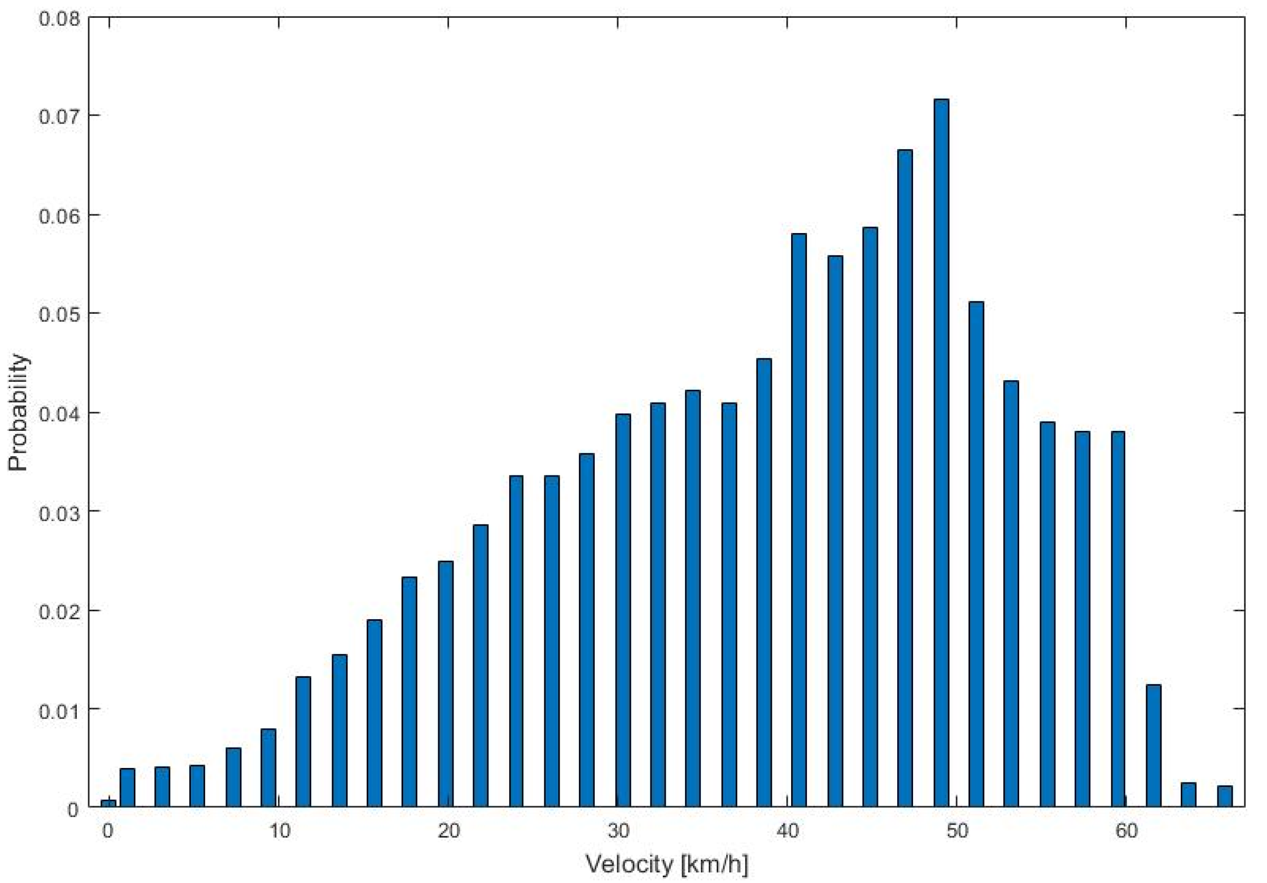
The average distributions of vehicle speeds (Figure 11) and TPM (Figure 12) were also recorded. The resolution of vehicle speeds was found to be 2.0875 km/h.
After the route was divided into segments consisting of groups of microtrips or grouped according to traffic volume, speed limit etc., the TPM was determined for each segment and boundary energy.
3.4. Simulation Results
This method is dedicated to autonomous vehicles or vehicles with an autopilot feature (driving in semiautonomous mode). The test route was divided into four segments. The TPM was used to generate the next state that determines speed and acceleration. This state can be interrupted at any time by road conditions and traffic. Thus, the TPM is corrected on an ongoing basis, assuming that microtrips between traffic lights are driven at the speed limit and acceleration is additionally limited by energy consumption.
The division into segments was made to illustrate the functioning of the algorithm. For a longer route, a single segment could be used due to the road conditions. The application of the method for a sample driving cycle is shown in Figure 13. The energy boundary was determined based on average energy consumption during the driving cycles by the eco-driver. The corrected cycle was determined by simulation. Figure 13a shows the uncorrected distance-based driving cycle (blue dashed line) for driving with the autopilot and a cycle corrected by the algorithm (red line). In Figure 13b, the energy boundary for each of the four segments and energy consumption during driving (from the beginning of the segment) are added for the corrected and uncorrected cycle.
Figure 14 shows the corrected and uncorrected cycle as a function of time.
Table 3 shows average energy consumption during each driving segment and for the entire cycle. Reduced speed and acceleration results in approximately 15% reduction of energy consumption, albeit an 82 s (approximately 10%) extension of travel time (without idling).
Electricity consumption should oscillate around the boundary energy because braking at the end of each segment provides an opportunity to recover some of the energy expended. In the first segment, the vehicle speed is corrected, but if energy consumption at the end of the segment exceeds the boundary energy—as is the case in the first segment—the next (second) segment begins with a correction of speed and acceleration. The correction is made only with accelerations because decelerations result in energy recovery. The correction is implemented only until energy consumption drops below the boundary energy. In the fourth segment, speed is initially corrected; then, later in two microtrips, both speed and acceleration are corrected. The last microtrip does not require any correction.
4. Conclusions
This article presents an adaptive method for optimizing the driving cycle with regard to energy consumption. Compared to methods used to develop representative driving cycles, the method described herein proposes distance-based driving cycles instead of time-based driving cycles. Driving cycles are segmented based on a driving cycle dataset. The next state, determined by speed and acceleration, is defined as the Markov chain next stage. However, this state can be disrupted by traffic conditions. Thus, TPM is updated on an ongoing basis and corrected where necessary if energy consumption is greater than assumed. Energy consumption during driving is monitored and compared with the assumed boundary energy. An autopilot driving cycle was verified in the study, with the cycle adapting to very restrictive limits on energy consumption. Speed or product of the speed and acceleration (va) were reduced when consumption was too high. Energy consumption was reduced by approximately 15%, although travel time was prolonged by approximately 10%.
The tests showed that driving was most energy-efficient at low speeds and accelerations (e.g., driving in congestion). However, many users would not regard this as the optimum driving cycle. It is also necessary to consider travel time, which is a significant aspect in the case of buses, and traffic flow, although this parameter cannot be measured directly. Further study should focus on the optimization criteria and the algorithm used to determine the energy boundary.
The study does not deal in detail with the energy consumption of HVAC systems. However, this energy has been statistically included in the design of the energy boundary. While the motor consumes no electricity during the idling phase, HVAC energy consumption is a real challenge in EV.
This paper is relevant to the topic of energy management in so-called intelligent public transport. Energy management is important for the transport of people (car-sharing, public bus transport) and goods (delivery vehicles).
Author Contributions
Conceptualization, I.K.; methodology, I.K. and A.P.; software, I.K.; validation, A.P. and A.N.; formal analysis, A.P.; investigation, M.Ś. and T.S.; resources, M.Ś.; data curation, T.S.; writing—original draft preparation, I.K.; writing—review and editing, I.K.; visualization, I.K.; supervision, A.N. All authors have read and agreed to the published version of the manuscript.
Funding
This research received no external funding.
Conflicts of Interest
The authors declare no conflict of interest.
Abbreviations
| DBADC | distance-based adaptive driving cycle |
| DC | driving cycle |
| EV | electric vehicle |
| GPR | Gaussian process regression |
| HEV | hybrid electric vehicle |
| HVAC | heating, ventilation and air-conditioning |
| MC | Markov chains |
| MCMC | Monte Carlo Markov chain |
| MLE | maximum likelihood estimation |
| PHEV | plug-in hybrid electric vehicle |
| SAPD | speed acceleration probability density |
| TPM | transition probability matrix |
| va | velocity and acceleration product |
References
- Ashtari, A.; Bibeau, E.; Shahidinejad, S. Using Large Driving Record Samples and a Stochastic Approach for Real-World Driving Cycle Construction: Winnipeg Driving Cycle. Transp. Sci. 2012, 48, 170–183. [Google Scholar] [CrossRef]
- Berzi, L.; Delogu, M.; Pierini, M. Development of driving cycles for electric vehicles in the context of the city of Florence. Transp. Res. Part D Transp. Environ. 2016, 47, 299–322. [Google Scholar] [CrossRef]
- Brady, J.; Mahony, M. Development of a driving cycle to evaluate the energy economy of electric vehicles in urban areas. Appl. Energy 2016, 177, 165–178. [Google Scholar] [CrossRef]
- Sun, Z.; Wen, Z.; Zhao, X.; Yang, Y.; Li, S. Real-World Driving Cycles Adaptability of Electric Vehicles. World Electr. Veh. J. 2020, 11, 19. [Google Scholar] [CrossRef] [Green Version]
- Yuan, X.; Zhang, C.; Hong, G.; Huang, X.; Li, L. Method for evaluating the real-world driving energy consumptions of electric vehicles. Energy 2017, 141, 1955–1968. [Google Scholar] [CrossRef]
- Liu, X.; Ma, J.; Zhao, X.; Du, J.; Xiong, Y. Study on Driving Cycle Synthesis Method for City Buses considering Random Passenger Load. J. Adv. Transp. 2020, 2020, 1–21. [Google Scholar] [CrossRef]
- Brundell, K.; Ericsson, E. Influence of street characteristics, driver category and car performance on urban driving patterns. Transp. Res. Part D Transp. Environ. 2005, 10, 213–229. [Google Scholar] [CrossRef]
- Hung, W.T.; Tong, H.Y.; Lee, C.P.; Ha, K.; Pao, L.Y. Development of a Practical Driving Cycle Construction Methodology: A Case Study in Hong Kong. Transp. Res. Part D Transp. Environ. 2007, 12, 115–128. [Google Scholar] [CrossRef]
- Borucka, A.; Wiśniowski, P.; Mazurkiewicz, D.; Świderski, A. Laboratory measurements of vehicle exhaust emissions in conditions reproducing real traffic. Measurement 2021, 174, 108998. [Google Scholar] [CrossRef]
- Chen, Z.; Zhang, Q.; Lu, J.; Bi, J. Optimization-based method to develop practical driving cycle for application in electric vehicle power management: A case study in Shenyang, China. Energy 2019, 186, 1157–1166. [Google Scholar] [CrossRef]
- Ma, R.; He, X.; Zheng, Y.; Zhou, B.; Lu, S.; Wu, Y. Real-world driving cycles and energy consumption informed by large-sized vehicle trajectory data. J. Clean. Prod. 2019, 223, 564–574. [Google Scholar] [CrossRef]
- Esser, A.; Zeller, M.; Foulard, S.; Rinderknecht, S. Stochastic Synthesis of Representative and Multidimensional Driving Cycles. SAE Int. 2018. [Google Scholar] [CrossRef]
- Desreveaux, A.; Bouscayrol, A.; Trigui, R.; Castex, E.; Klein, J. Impact of the Velocity Profile on Energy Consumption of Electric Vehicles. IEEE Trans. Veh. Technol. 2019, 68, 11420–11426. [Google Scholar] [CrossRef]
- Nyberg, P.; Frisk, E.; Nielsen, L. Generation of Equivalent Driving Cycles Using Markov Chains and Mean Tractive Force Components. IFAC Proc. 2014, 47, 8787–8792. [Google Scholar] [CrossRef] [Green Version]
- Semal, P. Monotone Iterative Methods for Markov Chains. Linear Algebra Its Appl. 1995, 230, 35–46. [Google Scholar] [CrossRef] [Green Version]
- Lee, T.-K.; Filipi, Z.S. Synthesis of Real-World Driving Cycles Using Stochastic Process and Statistical Methodology. Int. J. Veh. Des. 2011, 57, 17–36. [Google Scholar] [CrossRef]
- Gong, Q.; Midlam-Mohler, S.; Marano, V.; Rizzoni, G. An Iterative Markov Chain Approach for Generating Vehicle Driving Cycles. SAE Int. J. Engines 2011, 4, 1035–1045. [Google Scholar] [CrossRef]
- Souffran, G.; Miegeville, L.; Guerin, P. Simulation of Real-World Vehicle Missions Using a Stochastic Markov Model for Optimal Powertrain Sizing. IEEE Trans. Veh. Technol. 2012, 61, 3454–3465. [Google Scholar] [CrossRef]
- Silvas, E.; Hereijgers, K.; Peng, H.; Hofman, T.; Steinbuch, M. Synthesis of realistic driving cycles with high accuracy and computational speed, including slope information. IEEE Trans. Veh. Technol. 2016, 65, 4118–4128. [Google Scholar] [CrossRef]
- Zhao, B.; Hofman, T.; Lv, C.; Steinbuch, M. Intelligent synthesis of driving cycle for advanced design and control of powertrains. In Proceedings of the IEEE Intelligent Vehicles Symposium (IV) 2018, Changshu, China, 26–30 June 2018. [Google Scholar] [CrossRef]
- Puchalski, A.; Komorska, I.; Ślęzak, M.; Niewczas, A. Synthesis of naturalistic vehicle driving cycles using the Markov Chain Monte Carlo method. Eksploat. Niezawodn. Maint. Reliab. 2020, 22, 316–322. [Google Scholar] [CrossRef]
- Shi, S.; Nan, L.; Zhang, Y.; Chaosheng, H.; Liu, L.; Lu, B.; Cheng, J. Research on Markov property analysis of driving cycle. In Proceedings of the IEEE Vehicle Power and Propulsion Conference, Piscataway, NJ, USA, 10–18 October 2013; pp. 1–5. [Google Scholar]
- Zhang, M.; Shi, S.; Cheng, W.; Shen, Y. Self-Adaptive Hyper-Heuristic Markov Chain Evolution for Generating Vehicle Multi-Parameter Driving Cycles. IEEE Trans. Veh. Technol. 2020, 69, 6041–6052. [Google Scholar] [CrossRef]
- Lin, J.; Niemeier, D.A. Estimating Regional Air Quality Vehicle Emission Inventories: Constructing Robust Driving Cycles. Transp. Sci. 2003, 37, 330–346. [Google Scholar] [CrossRef] [Green Version]
- Borucka, A.; Niewczas, A.; Hasilova, K. Forecasting the readiness of special vehicles using the semi-Markov model. Eksploat. Niezawodn. Maint. Reliab. 2019, 21, 662–669. [Google Scholar] [CrossRef]
- Austin, T.C.; DiGenova, F.J.; Carlson, T.R.; Joy, R.W.; Gianlini, K.A.; Lee, J.M. Characterization of Driving Patterns and Emissions from Light-Duty Vehicles in California; Final Report 1993; Sierra Research Inc.: Street Sacramento, CA, USA, 1993. [Google Scholar] [CrossRef]
- Nesamani, K.S.; Subramanian, K.P. Development of a Driving Cycle for Intra-City Buses in Chennai, India. Atmos. Environ. 2011, 45, 5469–5476. [Google Scholar] [CrossRef]
- Zähringer, M.; Kalt, S.; Lienkamp, M. Compressed Driving Cycles Using Markov Chains for Vehicle Powertrain Design. World Electr. Veh. J. 2020, 11, 52. [Google Scholar] [CrossRef]
- Zhang, X.; Göhlich, D.; Li, J. Energy-Efficient Toque Allocation Design of Traction and Regenerative Braking for Distributed Drive Electric Vehicles. IEEE Trans. Veh. Technol. 2018, 67, 285–295. [Google Scholar] [CrossRef]
- Xu, W.; Chen, H.; Zhao, H.; Ren, B. Torque optimization control for electric vehicles with four in-wheel motors equipped with regenerative braking system. Mechatronics 2019, 57, 95–108. [Google Scholar] [CrossRef]
- Rasmussen, C.E.; Williams, C.K.I. Gaussian Processes for Machine Learning; MIT Press: Cambridge, MA, USA, 2006. [Google Scholar]
Figure 1.
Illustration of the DBADC method.

Figure 2.
A sample segment (a) velocity vs. time, (b) velocity vs. distance, (c) acceleration vs. time, (d) acceleration vs. distance.
Figure 2.
A sample segment (a) velocity vs. time, (b) velocity vs. distance, (c) acceleration vs. time, (d) acceleration vs. distance.

Figure 3.
Simulation of a sample driving cycle (a) and energy consumption (b) during a cycle with and without correction.
Figure 3.
Simulation of a sample driving cycle (a) and energy consumption (b) during a cycle with and without correction.

Figure 4.
Travel route.

Figure 5.
Recorded driving cycles (a) as a function of time, (b) as a function of travel distance for dynamic driving, eco-driving and autopilot.
Figure 5.
Recorded driving cycles (a) as a function of time, (b) as a function of travel distance for dynamic driving, eco-driving and autopilot.

Figure 6.
Verification of the GPR model: (a) the predicted responses and 95% prediction intervals using the fitted model, (b) zoom, (c) predicted vs. true response.
Figure 6.
Verification of the GPR model: (a) the predicted responses and 95% prediction intervals using the fitted model, (b) zoom, (c) predicted vs. true response.

Figure 7.
Simulated segments of the driving cycle as a function of distance (a) and corresponding energy consumption (b).
Figure 7.
Simulated segments of the driving cycle as a function of distance (a) and corresponding energy consumption (b).

Figure 8.
Comparison of driving cycle parameters for autopilot, eco-driving and dynamical driving: (a) percentage of time in speed ranges, (b) percentage of time in va ranges.
Figure 8.
Comparison of driving cycle parameters for autopilot, eco-driving and dynamical driving: (a) percentage of time in speed ranges, (b) percentage of time in va ranges.

Figure 9.
Cruising time (without idling) vs. average energy consumption.

Figure 10.
SAPD for investigated driving cycle.

Figure 11.
Average histogram of vehicle speeds on the tested route.

Figure 12.
Average probability transition matrix for driving cycles on the route investigated.

Figure 13.
Illustration of the method using the investigated driving cycle: (a) distance-based driving cycle, (b) electricity consumption at successive route segments.
Figure 13.
Illustration of the method using the investigated driving cycle: (a) distance-based driving cycle, (b) electricity consumption at successive route segments.

Figure 14.
Time-based driving cycles for Figure 13a.
Figure 14.
Time-based driving cycles for Figure 13a.

Figure 15.
Comparison of electricity consumption in the uncorrected and corrected cycle in relation to the assumed boundary energy in each segment and in the overall cycle.
Figure 15.
Comparison of electricity consumption in the uncorrected and corrected cycle in relation to the assumed boundary energy in each segment and in the overall cycle.


Table 1.
The calculated parameters in driving cycles.
| Number | Parameter |
|---|---|
| 1 | Average speed |
| 2 | Average speed (only cruising) |
| 3 | Standard deviation of speed |
| 4 | Maximum acceleration |
| 5 | Average acceleration |
| 6 | Standard deviation of acceleration |
| 7 | Maximum deceleration |
| 8 | Average deceleration |
| 9 | Standard deviation of deceleration |
| 10 | % of time when idling |
| 11 | % of time when speed is 0–15 (km·h−1) |
| 12 | % of time when speed is 15–30 (km·h−1) |
| 13 | % of time when speed is 30–50 (km·h−1) |
| 14 | % of time when speed is >50 (km·h−1) |
| 15 | % of time when va 1 is <0 (m2·s−3) |
| 16 | % of time when va is 0–3 (m2·s−3) |
| 17 | % of time when va is 3–6 (m2·s−3) |
| 18 | % of time when va is 6–10 (m2·s−3) |
| 19 | % of time when va is >10 (m2·s−3) |
| 20 | Total duration |
| 21 | Time of cruising without idling |
| 22 | Average energy consumption |
1 va is the product of vehicle velocity and acceleration.
Table 2.
Driving cycle parameters.
| No. | Parameter | Dynamical Driving | Eco-Driving | Autopilot |
|---|---|---|---|---|
| 1 | Average speed | 22.90 | 19.86 | 19.06 |
| 2 | Average speed (only cruising) | 35.15 | 29.03 | 28.84 |
| 3 | Standard deviation of speed | 25.45 | 19.38 | 19.32 |
| 4 | Maximum acceleration | 5.69 | 2.43 | 2.20 |
| 5 | Average acceleration | 1.18 | 0.62 | 0.62 |
| 6 | Standard deviation of acceleration | 0.47 | 0.48 | 0.47 |
| 7 | Maximum deceleration | −4.22 | −2.61 | −3.12 |
| 8 | Average deceleration | −0.95 | −0.63 | −0.67 |
| 9 | Standard deviation of deceleration | 0.74 | 0.47 | 0.55 |
| 10 | % of time when idling | 36.7 | 33.3 | 35.9 |
| 11 | % of time when speed is 0–15 (km·h−1) | 13.5 | 15.1 | 14.9 |
| 12 | % of time when speed is 15–30 (km·h−1) | 15.2 | 18.3 | 17.4 |
| 13 | % of time when speed is 30–50 (km·h−1) | 17.0 | 24.8 | 24.8 |
| 14 | % of time when speed is >50 (km·h−1) | 17.6 | 8.5 | 7.0 |
| 15 | % of time when va1 is <0 (m2·s−3) | 33.6 | 31.8 | 29.1 |
| 16 | % of time when va is 0–3 (m2·s−3) | 8.5 | 15.1 | 14.7 |
| 17 | % of time when va is 3–6 (m2·s−3) | 5.7 | 9.9 | 9.1 |
| 18 | % of time when va is 6–10 (m2·s−3) | 4.1 | 5.7 | 5.8 |
| 19 | % of time when va is >10 (m2·s−3v | 10.9 | 3.2 | 3.8 |
| 20 | Total duration (s) | 999.3 | 1147.2 | 1214.0 |
| 21 | Time of cruising without idling (s) | 648.8 | 780.5 | 789.0 |
| 22 | Average energy consumption (Wh·km−1) | 427.6 | 260.7 | 309.4 |
Table 3.
Comparison of average electricity consumption during driving in each segment in relation to the assumed boundary energy.
Table 3.
Comparison of average electricity consumption during driving in each segment in relation to the assumed boundary energy.
| Parameter | Segment 1 | Segment 2 | Segment 3 | Segment 4 | Total | Difference % |
|---|---|---|---|---|---|---|
| Distance (km) | 1.858 | 1.425 | 1.067 | 2.016 | 6.366 | |
| Average energy for autopilot (Wh/km) | 285.5 | 314.8 | 237.0 | 302.7 | 289.4 | 11.0 |
| Average boundary energy (Wh/km) | 259.6 | 276.8 | 278.3 | 241.1 | 260.7 | 0 |
| Average energy for cycle with correction (Wh/km) | 266.0 | 267.1 | 228.4 | 224.7 | 246.9 | −5.3 |
Publisher’s Note: MDPI stays neutral with regard to jurisdictional claims in published maps and institutional affiliations. |
© 2021 by the authors. Licensee MDPI, Basel, Switzerland. This article is an open access article distributed under the terms and conditions of the Creative Commons Attribution (CC BY) license (https://creativecommons.org/licenses/by/4.0/).
Share and Cite
MDPI and ACS Style
Komorska, I.; Puchalski, A.; Niewczas, A.; Ślęzak, M.; Szczepański, T. Adaptive Driving Cycles of EVs for Reducing Energy Consumption. Energies 2021, 14, 2592. https://0-doi-org.brum.beds.ac.uk/10.3390/en14092592
AMA Style
Komorska I, Puchalski A, Niewczas A, Ślęzak M, Szczepański T. Adaptive Driving Cycles of EVs for Reducing Energy Consumption. Energies. 2021; 14(9):2592. https://0-doi-org.brum.beds.ac.uk/10.3390/en14092592
Chicago/Turabian StyleKomorska, Iwona, Andrzej Puchalski, Andrzej Niewczas, Marcin Ślęzak, and Tomasz Szczepański. 2021. "Adaptive Driving Cycles of EVs for Reducing Energy Consumption" Energies 14, no. 9: 2592. https://0-doi-org.brum.beds.ac.uk/10.3390/en14092592
Note that from the first issue of 2016, this journal uses article numbers instead of page numbers. See further details here.