
The Impact of System Integration on System Costs of a Neighborhood Energy and Water System

 and
and
Abstract
:
1. Introduction
1.1. Motivation
1.2. Literature Research
1.3. Focus of the Study
- -
- Consider 100% renewable systems, so excluding fossil sources, such as natural gas;
- -
- Taking into account multiple consumption sectors in a neighborhood (electricity, heating of buildings, mobility and water);
- -
- Hydrogen can be used for more purposes than electricity only, as it can also be applied in both the transport sector and for buildings (heating and electricity purposes);
- -
- Seasonal heat storage can contribute considerably to the large seasonal, temporal mismatch.
What is the impact of different modes of system integration on the local energy and water use, energy imports and exports, peaks in demand and supply and system costs for a neighborhood energy and water system?
2. Modeling Methodology
2.1. Rule-Based Scheduling Strategy
2.2. Economic Calculations
3. Neighborhood Scenarios
3.1. Design Choices
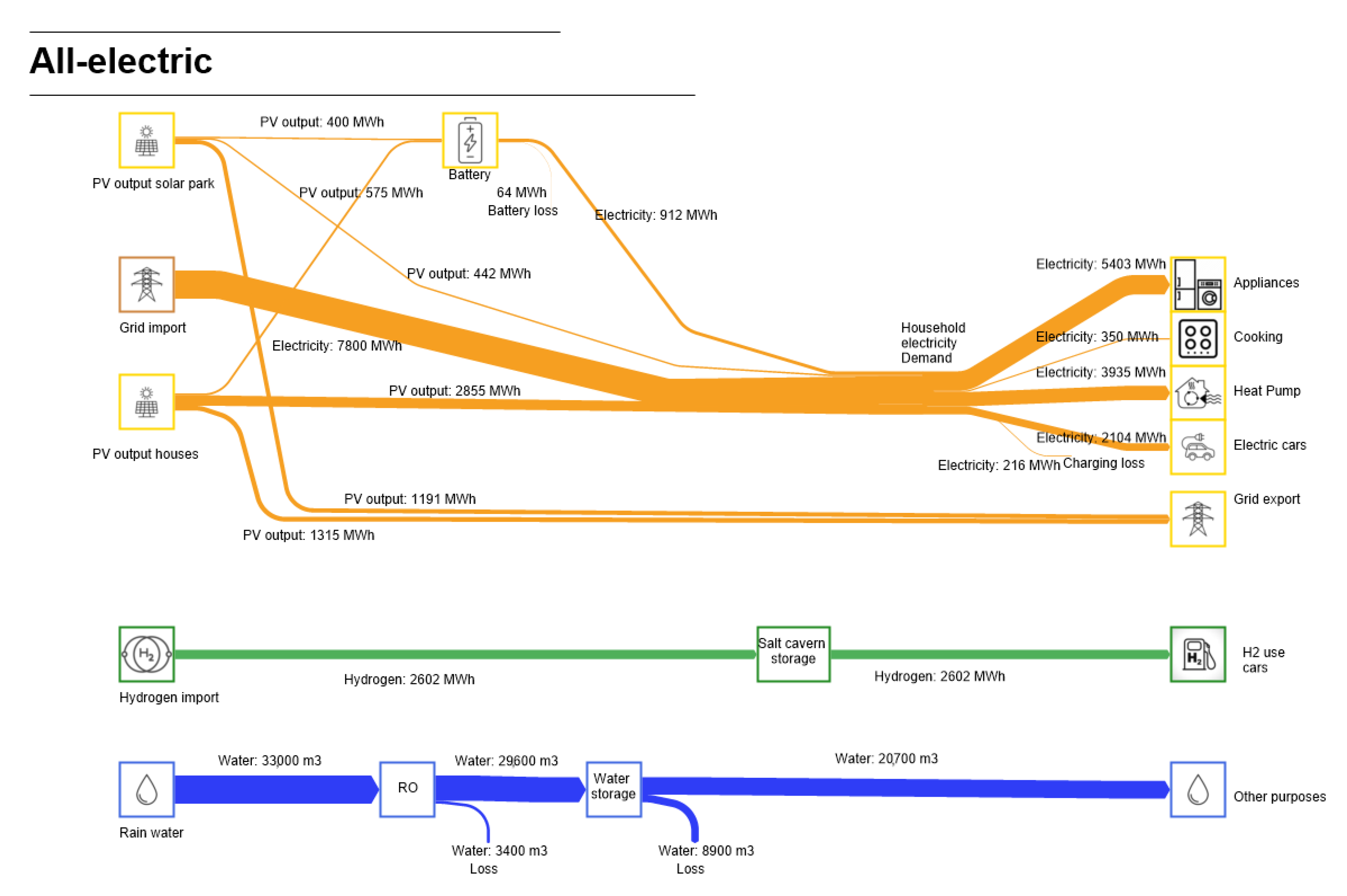
3.2. All-Electric
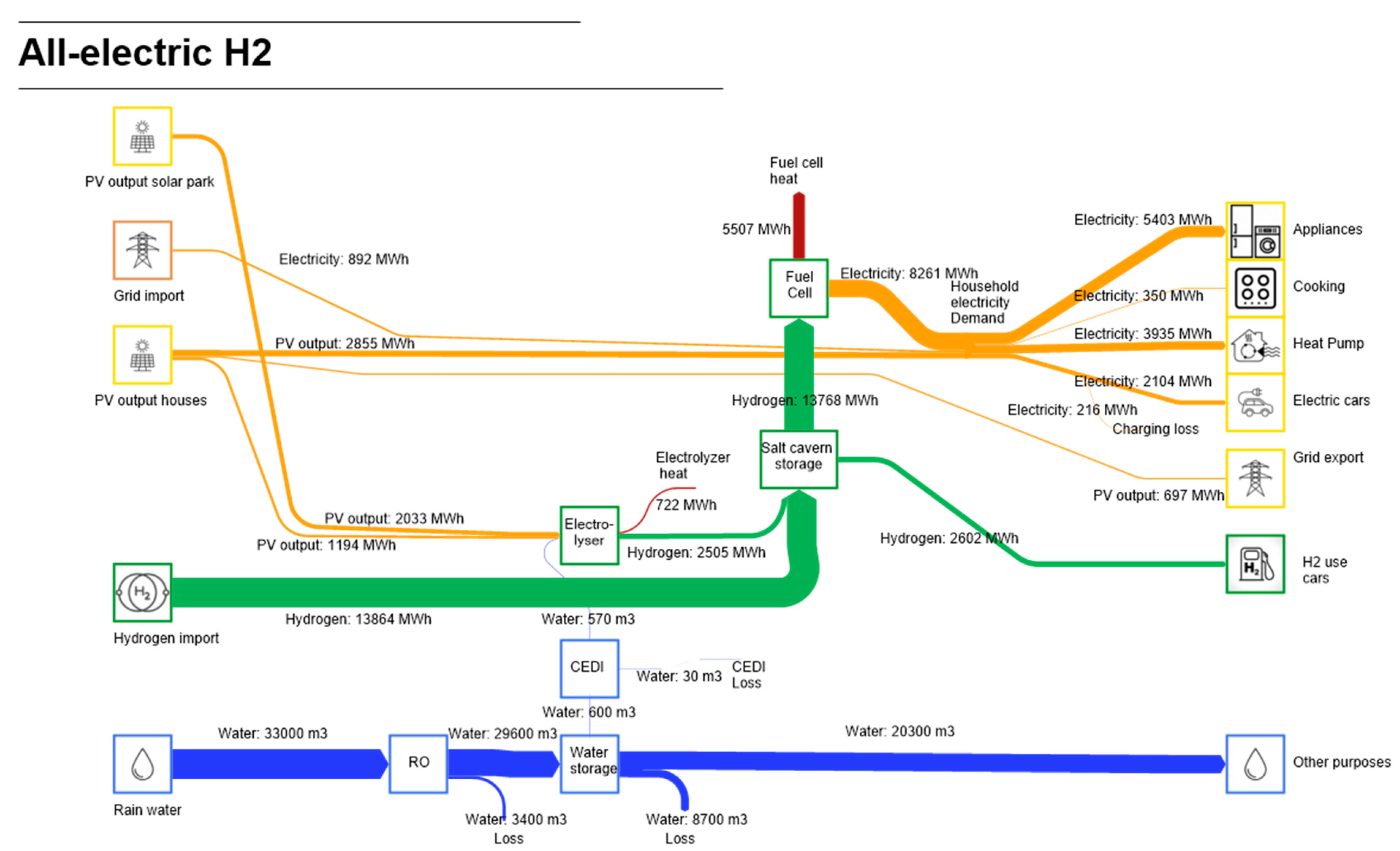
3.3. All-Electric H2
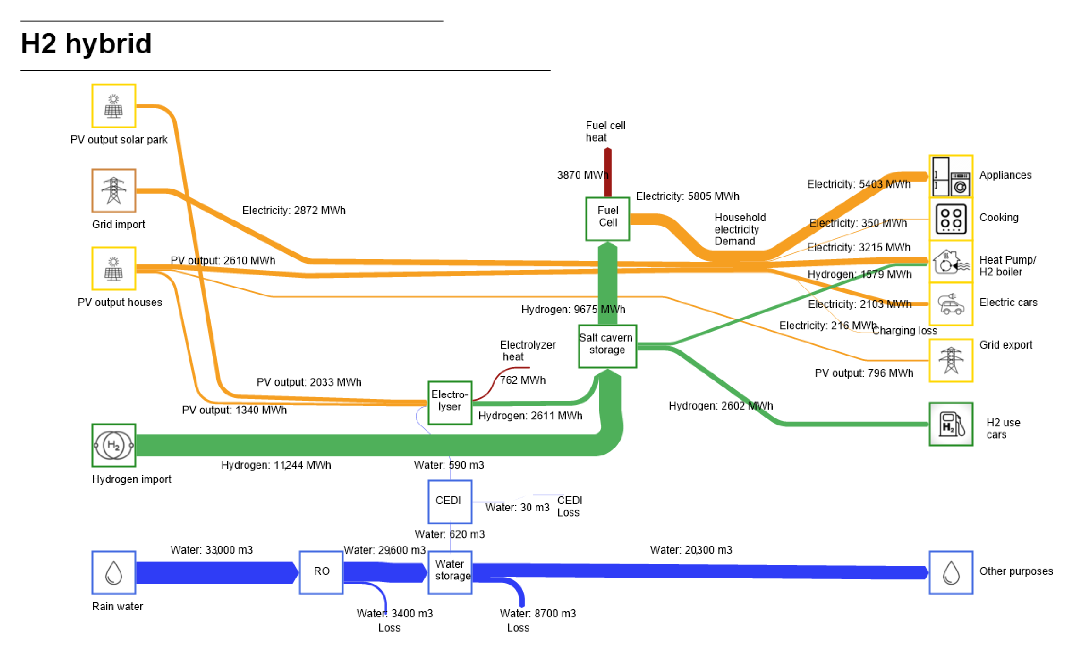
3.4. H2 Hybrid
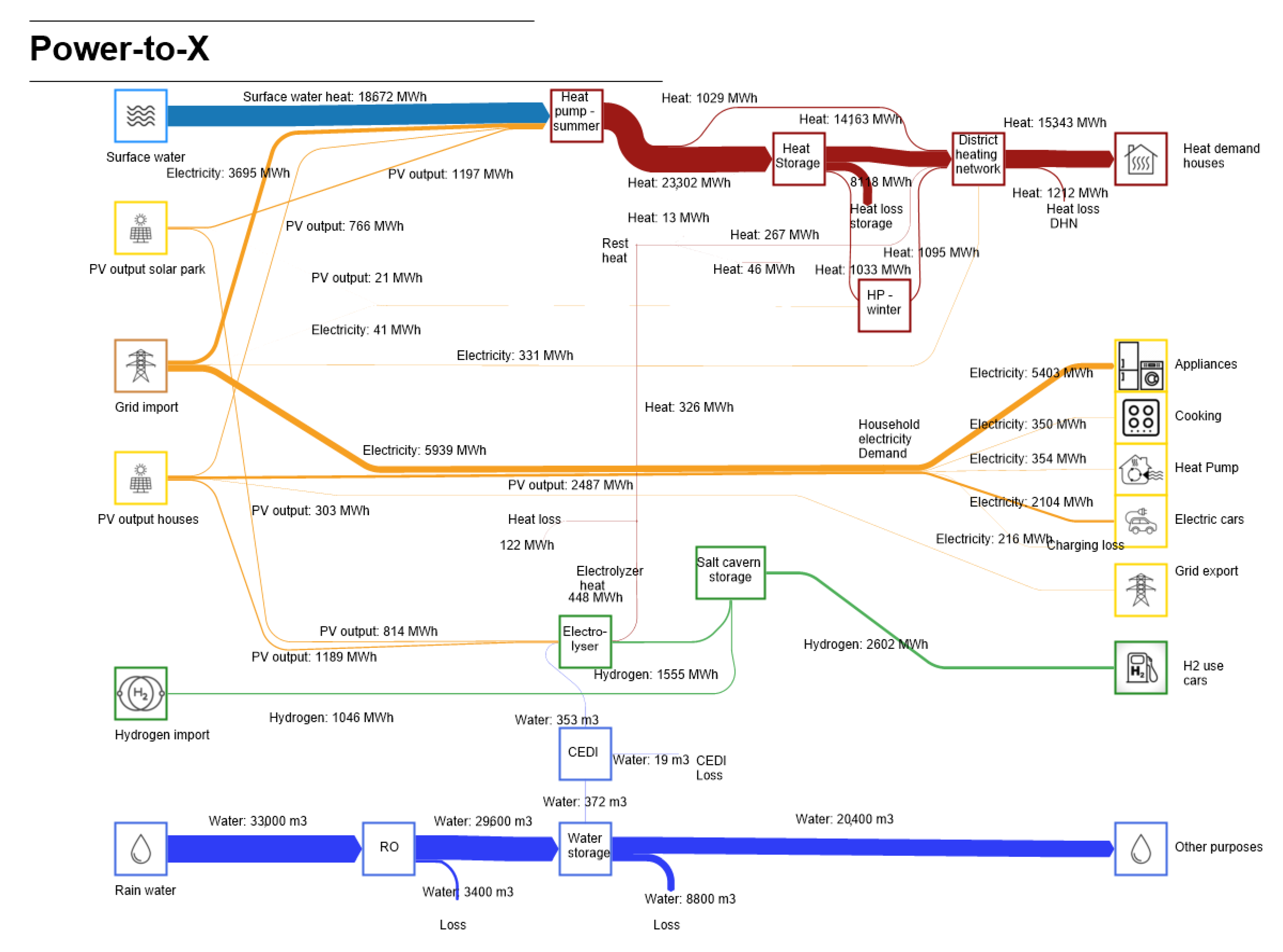
3.5. Power-to-X
4. Results
4.1. Local Energy and WATER USE
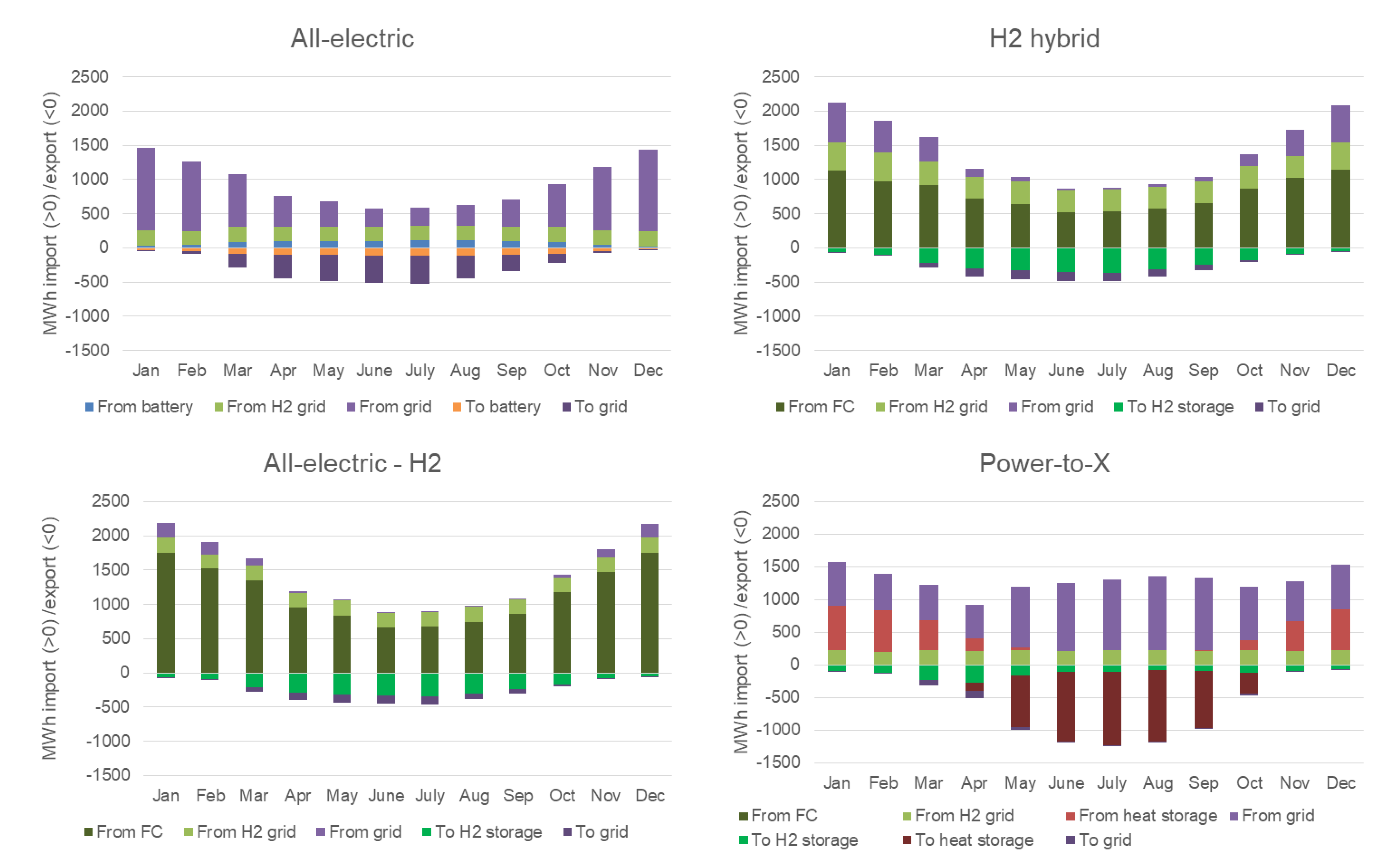
4.2. Import and Export of Energy
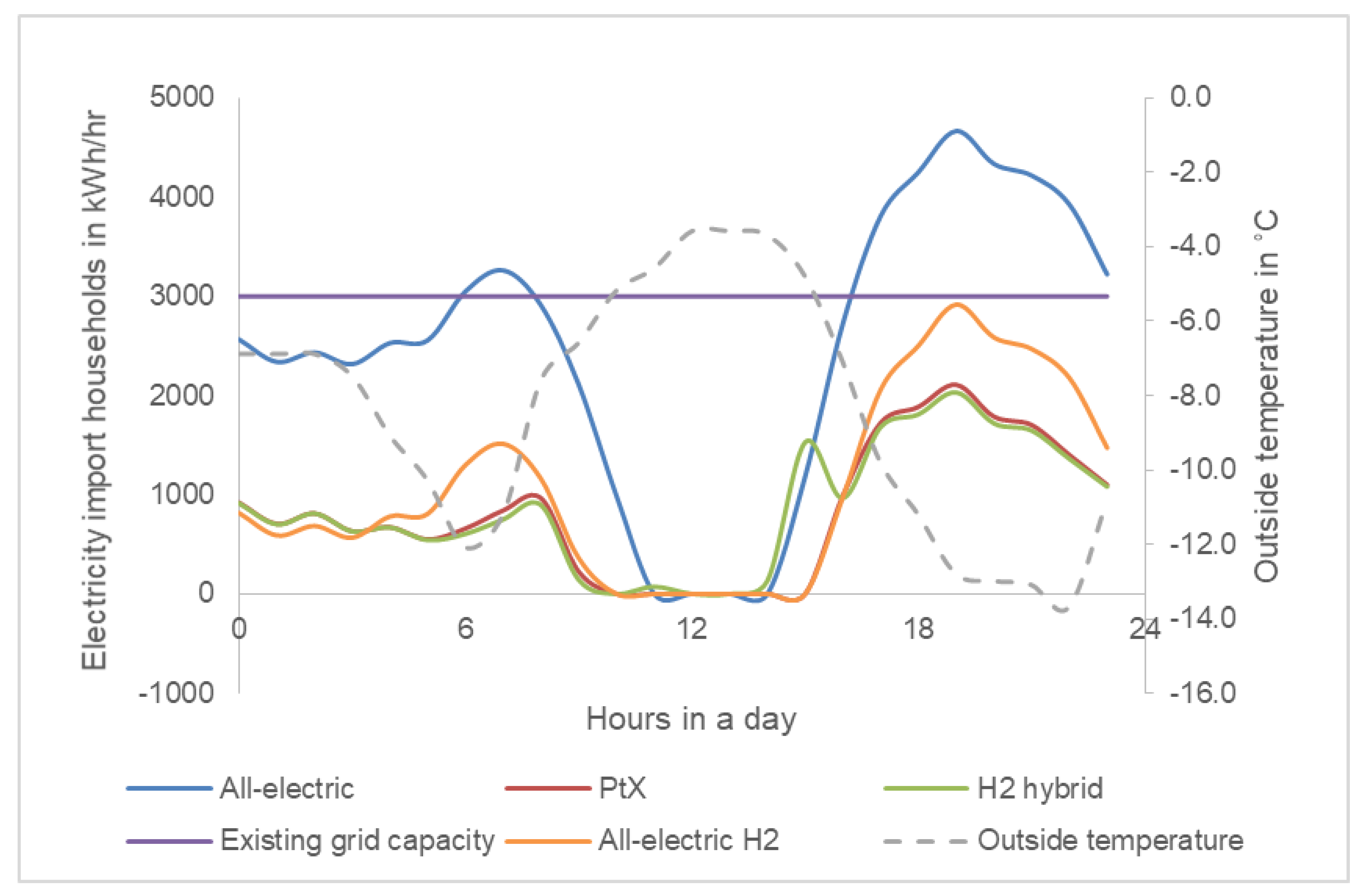
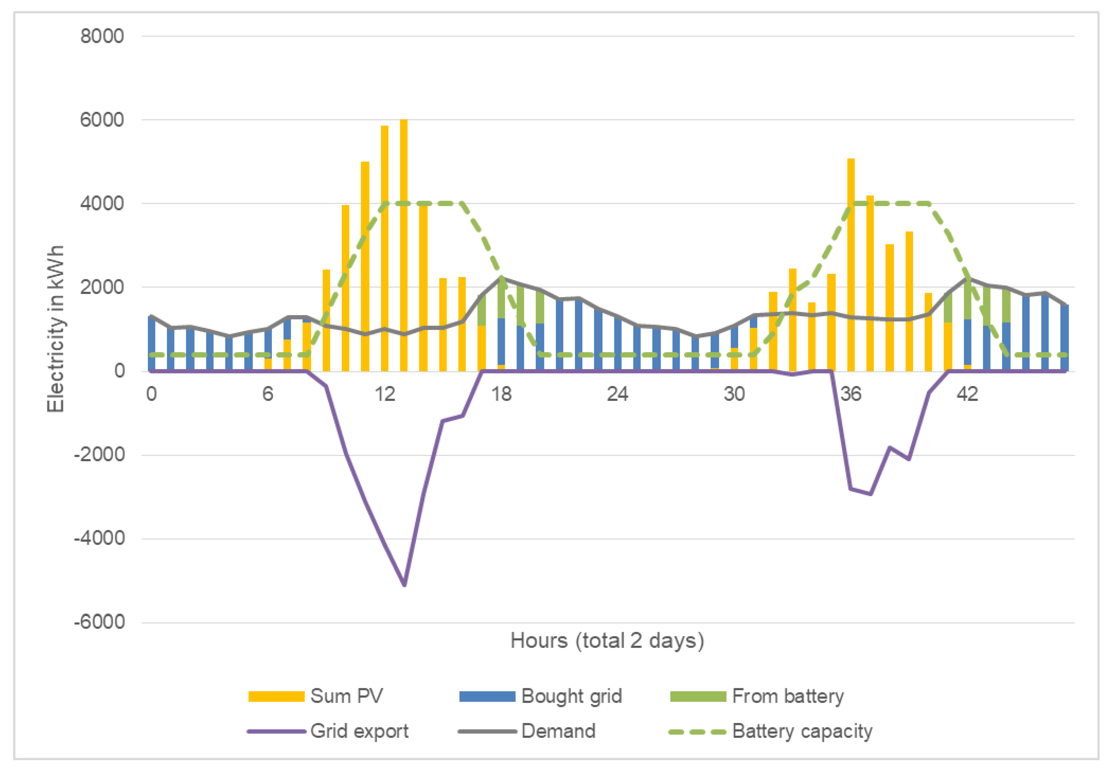
4.3. Peaks in Energy Demand and Supply
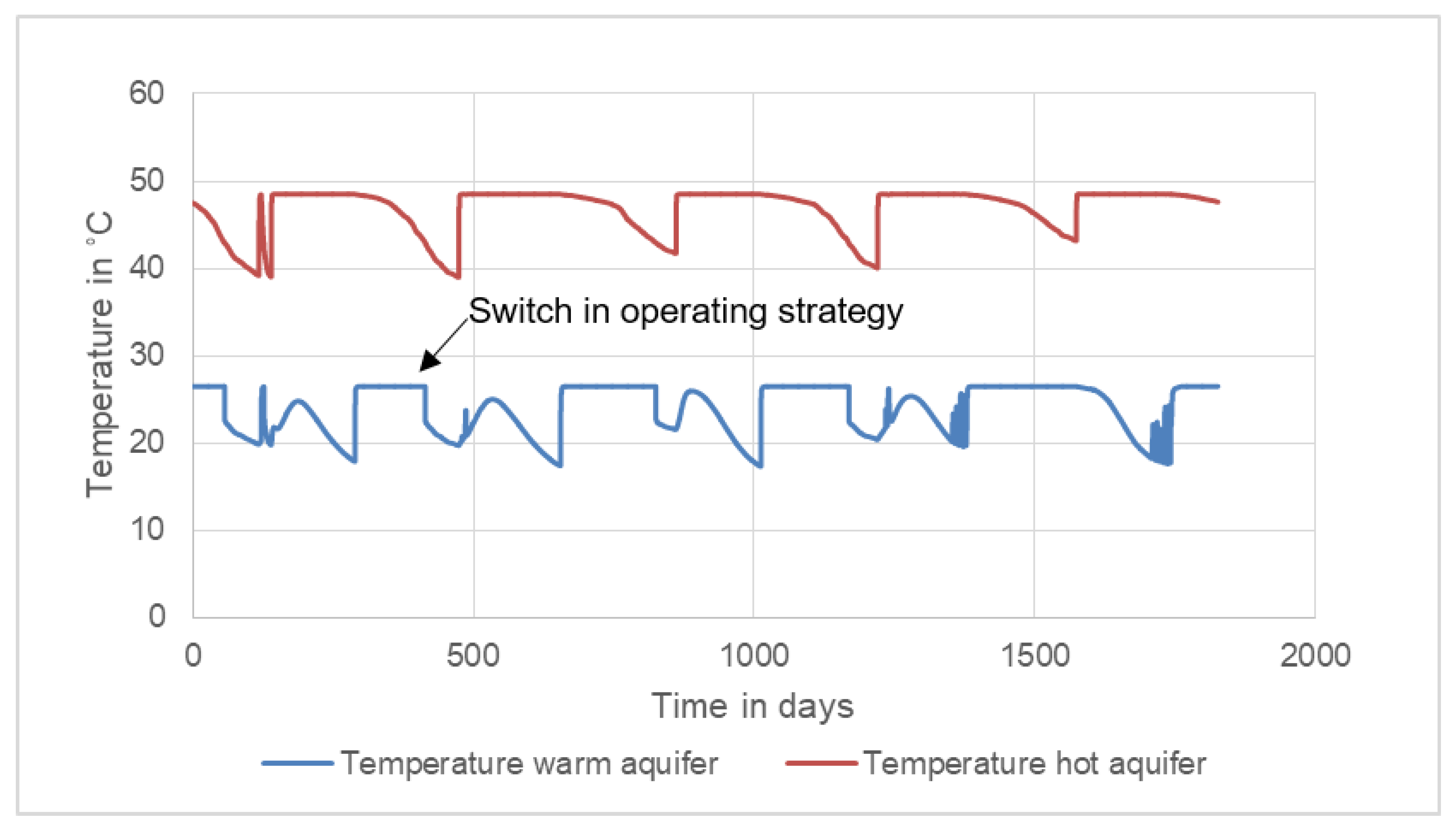
4.4. Zooming in on Long-Term Heat Storage
4.5. Economic Results
5. Discussion
5.1. Energy Balance
5.1.1. Local Production versus Energy Import
5.1.2. More Stable Energy Distribution Pattern with HT-ATES
5.1.3. The Impact of Electrolyzer and Fuel Cell Heat Integration on the Energy Balance
5.1.4. HT-ATES Recovery Efficiency
5.2. Water Supply and Possible Water Demands
5.2.1. Rainwater Supply and Storage in the Neighborhood
5.2.2. Possible Water Demands
5.3. Peak Demand and Supply
5.3.1. The Effect of Power-to-Hydrogen on Peak Demand
5.3.2. More Potential for Peak Shaving with Power-to-Heat and Power-to-Hydrogen
5.3.3. Other Flexibility Services of Power-to-Heat and Power-to-Hydrogen
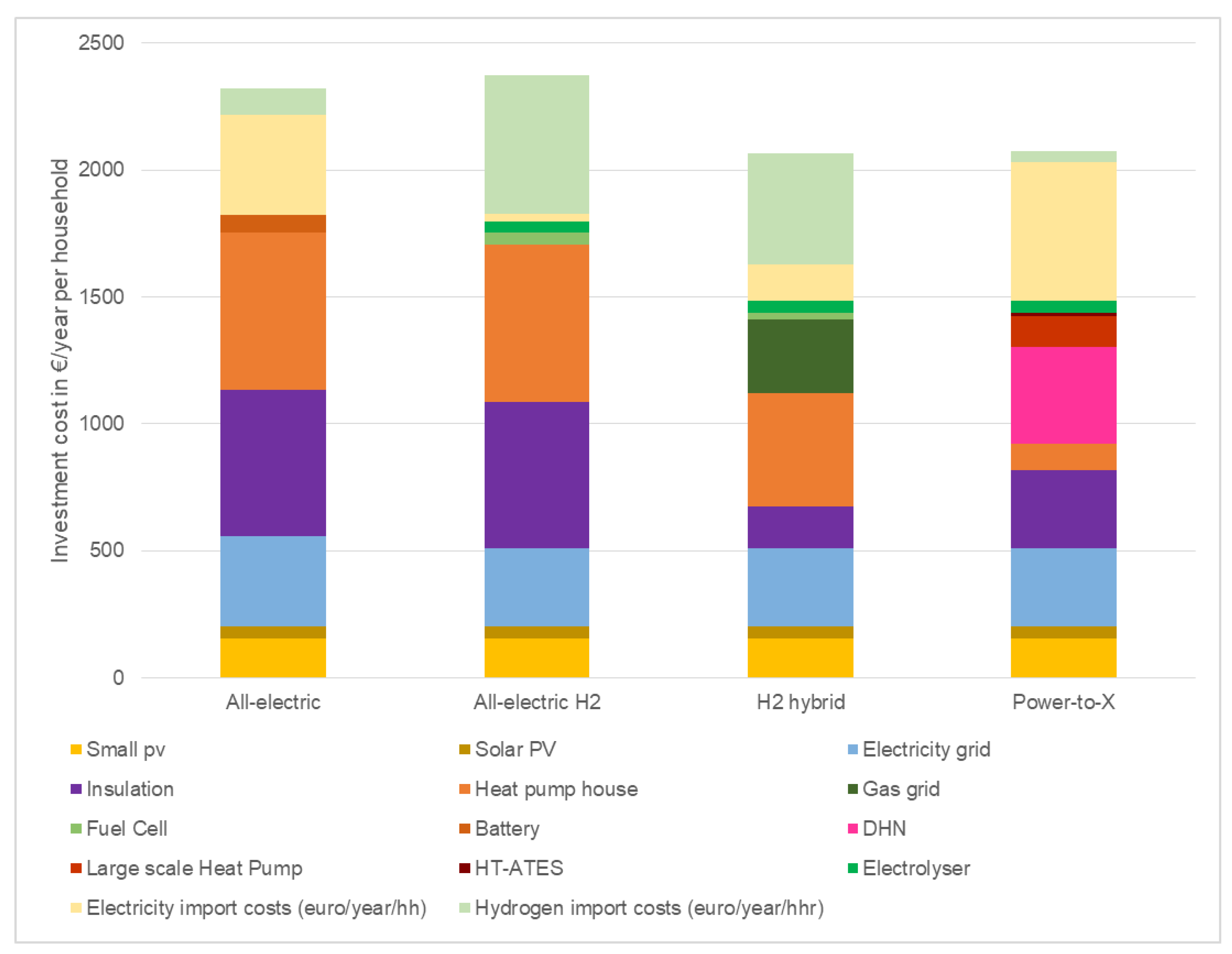
5.4. System Costs
5.4.1. Diversification of Energy Carriers Lead to Lower System Costs
5.4.2. Retrofitting as an Important Factor in Energy System Costs
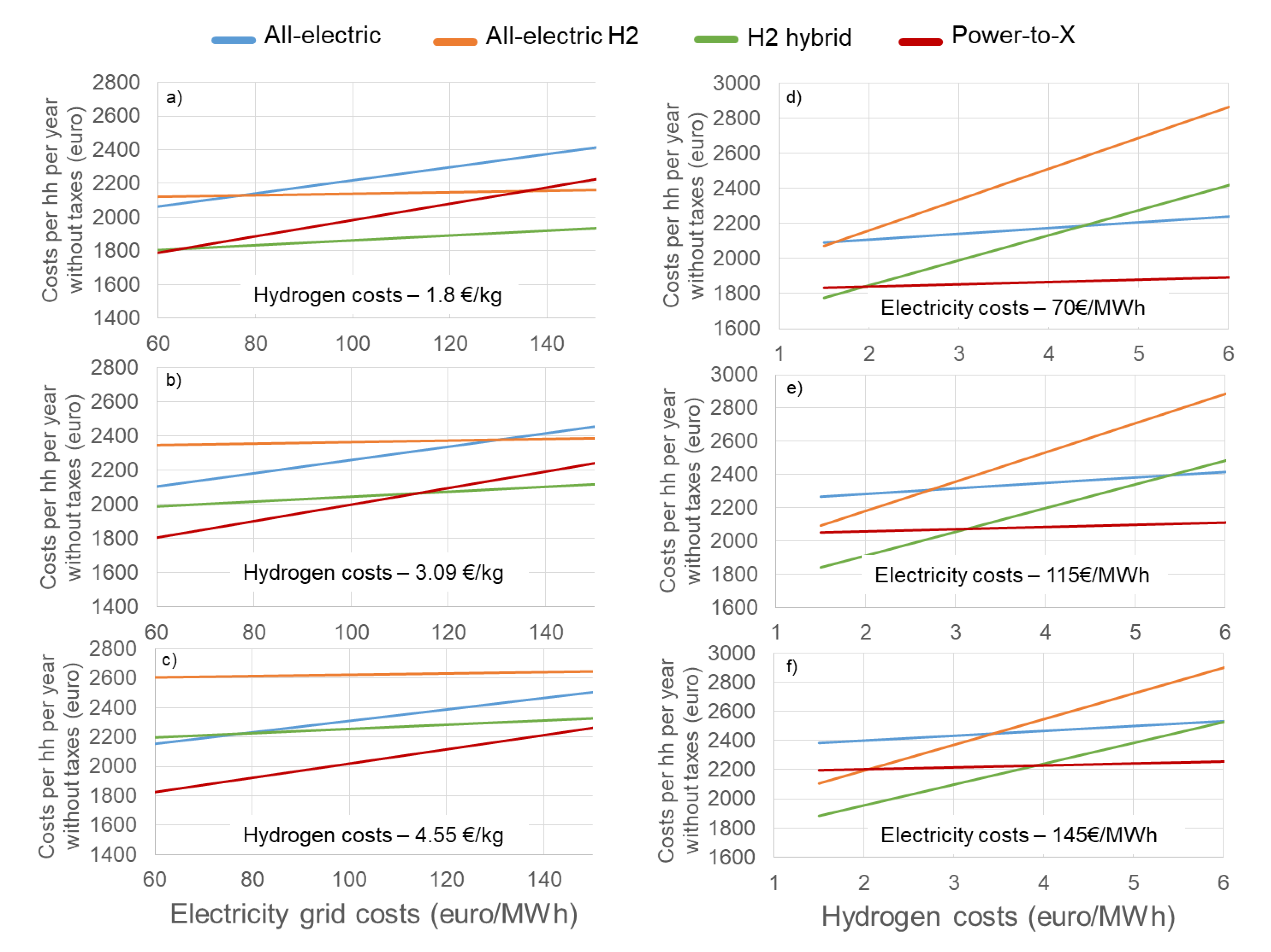
5.4.3. Local Hydrogen Production to Electricity Is More Expensive Than Using Electricity Directly
5.4.4. The Importance of Hybrid Designs
6. Conclusions
Supplementary Materials
Author Contributions
Funding
Data Availability Statement
Conflicts of Interest
Abbreviations
| BEV | Battery electric vehicle |
| CAPEX | Capital expenditures |
| COP | Coefficient of performance |
| CHP | Combined heat and power |
| DHN | District heating network |
| DOD | Depth of discharge |
| FCEV | Fuel cell electric vehicle |
| HHV | Higher heating value |
| HT-ATES | High-temperature aquifer thermal energy storage |
| kW | Kilowatt |
| MILP | Mixed-integer linear programming model |
| MW | Megawatt |
| GW | Gigawatt |
| OPEX | Operating expenditures |
| PV | Photovoltaic |
| RES | Renewable energy systems |
| Subscripts | |
| el | electric power |
| th | thermal power |
References
- REN21. Renewables 2020 Global Status Report; REN21 Secretariat: Paris, France, 2020; ISBN 978-3-948393-00-7. [Google Scholar]
- European Energy Agency. Trends and Projections in Europe 2019; Publications Office of the European Union: Luxembourg, 2019; ISBN 9789294801036. [Google Scholar]
- European Commission. The European Green Deal. Eur. Comm. 2019, 53, 24. [Google Scholar] [CrossRef]
- IEA. Power Systems in Transition; IEA: Paris, France, 2020. [Google Scholar]
- REN21. Renewables Global Futures Report; REN21: Paris, France, 2017; ISBN 9783981810745. [Google Scholar]
- Parag, Y.; Sovacool, B.K. Electricity market design for the prosumer era. Nat. Energy 2016, 1, 16032. [Google Scholar] [CrossRef]
- European Commission. Powering a Climate-Neutral Economy: An EU Strategy for Energy System Integration; European Commission: Brussel, Belgium, 2020. [Google Scholar]
- Robinius, M.; Otto, A.; Heuser, P.; Welder, L.; Syranidis, K.; Ryberg, D.; Grube, T.; Markewitz, P.; Peters, R.; Stolten, D. Linking the Power and Transport Sectors—Part 1: The Principle of Sector Coupling. Energies 2017, 10, 956. [Google Scholar] [CrossRef] [Green Version]
- Renewable Energy Policy Network. Renewables 2018 Global Status Report; REN21: Paris, France, 2018; ISBN 9783981891133. [Google Scholar]
- IRENA. Electricity Storage and Renewables: Costs and Markets to 2030; IRENA: Abu Dhabi, UAE, 2017. [Google Scholar]
- IEA. Technology Roadmap: Energy Storage; IEA: Paris, France, 2014. [Google Scholar]
- European Commission; Undertaking, F.C.H.J. Commercialisation of Energy Storage; European Commision: Brussel, Belgium, 2015. [Google Scholar]
- Mathiesen, B.V.; Lund, H.; Connolly, D.; Wenzel, H.; Ostergaard, P.A.; Möller, B.; Nielsen, S.; Ridjan, I.; KarnOe, P.; Sperling, K.; et al. Smart Energy Systems for coherent 100% renewable energy and transport solutions. Appl. Energy 2015, 145, 139–154. [Google Scholar] [CrossRef]
- Knowledge for Climate Climate Proof Cities. 2014.
- Oldenbroek, V.; Verhoef, L.A.; van Wijk, A.J.M. Fuel cell electric vehicle as a power plant: Fully renewable integrated transport and energy system design and analysis for smart city areas. Int. J. Hydrog. Energy 2017, 42, 8166–8196. [Google Scholar] [CrossRef]
- Robledo, C.B.; Oldenbroek, V.; Abbruzzese, F.; van Wijk, A.J.M. Integrating a hydrogen fuel cell electric vehicle with vehicle-to-grid technology, photovoltaic power and a residential building. Appl. Energy 2018, 215, 615–629. [Google Scholar] [CrossRef]
- Robinius, M.; Otto, A.; Syranidis, K.; Ryberg, D.S.; Heuser, P.; Welder, L.; Grube, T.; Markewitz, P.; Tietze, V.; Stolten, D. Linking the Power and Transport Sectors—Part 2: Modelling a Sector Coupling Scenario for Germany. Energies 2017, 10, 957. [Google Scholar] [CrossRef] [Green Version]
- Nastasi, B.; Lo Basso, G. Hydrogen to link heat and electricity in the transition towards future Smart Energy Systems. Energy 2016, 110, 5–22. [Google Scholar] [CrossRef]
- Orehounig, K.; Evins, R.; Dorer, V. Integration of decentralized energy systems in neighbourhoods using the energy hub approach. Appl. Energy 2015, 154, 277–289. [Google Scholar] [CrossRef]
- Wouters, C.; Fraga, E.S.; James, A.M. An energy integrated, multi-microgrid, MILP (mixed-integer linear programming) approach for residential distributed energy system planning—A South Australian case-study. Energy 2015, 85, 30–44. [Google Scholar] [CrossRef] [Green Version]
- Siraganyan, K.; Dasun Perera, A.T.; Scartezzini, J.L.; Mauree, D. Eco-SiM: A parametric tool to evaluate the environmental and economic feasibility of decentralized energy systems. Energies 2019, 12, 1–22. [Google Scholar] [CrossRef] [Green Version]
- Bloess, A.; Schill, W.P.; Zerrahn, A. Power-to-heat for renewable energy integration: A review of technologies, modeling approaches, and flexibility potentials. Appl. Energy 2018, 212, 1611–1626. [Google Scholar] [CrossRef]
- Gabrielli, P.; Gazzani, M.; Martelli, E.; Mazzotti, M. Optimal design of multi-energy systems with seasonal storage. Appl. Energy 2018, 219, 408–424. [Google Scholar] [CrossRef]
- Petkov, I.; Gabrielli, P.; Spokaite, M. The impact of urban district composition on storage technology reliance: Trade-offs between thermal storage, batteries, and power-to-hydrogen. Energy 2021, 224, 120102. [Google Scholar] [CrossRef]
- Murray, P.; Orehounig, K.; Grosspietsch, D.; Carmeliet, J. A comparison of storage systems in neighbourhood decentralized energy system applications from 2015 to 2050. Appl. Energy 2018, 231, 1285–1306. [Google Scholar] [CrossRef]
- Maroufmashat, A.; Fowler, M.; Sattari Khavas, S.; Elkamel, A.; Roshandel, R.; Hajimiragha, A. Mixed integer linear programing based approach for optimal planning and operation of a smart urban energy network to support the hydrogen economy. Int. J. Hydrog. Energy 2016, 41, 7700–7716. [Google Scholar] [CrossRef]
- van der Roest, E.; Snip, L.; Fens, T.; van Wijk, A. Introducing Power-to-H3: Combining renewable electricity with heat, water and hydrogen production and storage in a neighbourhood. Appl. Energy 2020, 257. [Google Scholar] [CrossRef]
- Brown, T.; Schlachtberger, D.; Kies, A.; Schramm, S.; Greiner, M. Synergies of sector coupling and transmission reinforcement in a cost-optimised, highly renewable European energy system. Energy 2018, 160, 720–739. [Google Scholar] [CrossRef] [Green Version]
- Walker, S.; Labeodan, T.; Boxem, G.; Maassen, W.; Zeiler, W. An assessment methodology of sustainable energy transition scenarios for realizing energy neutral neighborhoods. Appl. Energy 2018, 228, 2346–2360. [Google Scholar] [CrossRef]
- Drijver, B.; Van Aarssen, M.; Zwart, B. De High-temperature aquifer thermal energy storage (HT-ATES): Sustainable and multi-usable. In Proceedings of the Innostock 2012—12th International Conference on Energy Storage, Lleida, Spain, 16–18 May 2012; Volume 1, pp. 1–10. [Google Scholar]
- Wesselink, M.; Liu, W.; Koornneef, J.; van den Broek, M. Conceptual market potential framework of high temperature aquifer thermal energy storage—A case study in the Netherlands. Energy 2018, 147, 477–489. [Google Scholar] [CrossRef]
- Hartog, N.; Bloemendal, M.; Slingerland, E.; van Wijk, A. Duurzame Warmte Gaat Ondergronds; KWR: Utrecht, The Netherlands, 2016. [Google Scholar]
- McKenna, R.; Fehrenbach, D.; Merkel, E. The role of seasonal thermal energy storage in increasing renewable heating shares: A techno-economic analysis for a typical residential district. Energy Build. 2019, 187, 38–49. [Google Scholar] [CrossRef]
- Bloemendal, M.; Hartog, N. Thermal Energy Storage with geothermal triplet for space heating and cooling. In Proceedings of the EGU General Assembly 2017, Vienna, Austria, 23–28 April 2017. [Google Scholar]
- Bloemendal, M.; Van Wijk, A.; Hartog, N. Verwarming en koeling zonder warmtepomp met WKO-triplet. H2O, 2017; 1–9. [Google Scholar]
- HOMER Energy How HOMER Calculates the PV Array Power Output. Available online: https://www.homerenergy.com/products/grid/docs/1.5/how_homer_calculates_the_pv_array_power_output.html (accessed on 21 November 2020).
- IEA. The Future of Hydrogen; IEA: Paris, France, 2019. [Google Scholar]
- Dorin. Dorin software; Dorin: Compiobbi, Italy, 2018. [Google Scholar]
- Ruhnau, O.; Hirth, L.; Praktiknjo, A. Time series of heat demand and heat pump efficiency for energy system modeling. Sci. Data 2019, 6, 189. [Google Scholar] [CrossRef]
- Zuurbier, K.; van Dooren, T. Urban Waterbuffer Spangen: Resultaten; KWR: Utrecht, The Netherlands, 2019. [Google Scholar]
- Mongird, K.; Viswanathan, V.; Balducci, P.; Alam, J.; Fotedar, V.; Koritarov, V.; Hadjerioua, B. Energy Storage Technology and Cost Characterization Report; Department of Energy: Washington, DC, USA, 2019. [Google Scholar]
- Farahani, S.S.; Bleeker, C.; van Wijk, A.; Lukszo, Z. Hydrogen-based integrated energy and mobility system for a real-life office environment. Appl. Energy 2020, 264, 114695. [Google Scholar] [CrossRef]
- Fraunhofer ISE. Current and Future Cost of Photovoltaics: Long-Term Scenarios for Market Development; Fraunhofer ISE: Freiburg, Germany, 2015. [Google Scholar]
- Vartiainen, E.; Masson, G.; Breyer, C. PV LCOE in Europe 2014-2030, final report, 23 June 2015. 2015. [Google Scholar]
- Goldman Sachs. NextGen Power: Solar to Transform Europe’ s Energy Mix; Goldman Sachs: New York, NY, USA, 2018. [Google Scholar]
- Hydrogen Europe. Technology Roadmaps Full Pack; Hydrogen Europe: Brussels, Belgium, 2018. [Google Scholar]
- Van Wijk, A.; Chatzimarkakis, J. Green Hydrogen for a European Green Deal—A 2x40 GW Initiative; Hydrogen Europe: Brussels, Belgium, 2020. [Google Scholar]
- EnergiNet. The Danish Energy Agency Technology Data—Generation of Electricity and District Heating; EnergiNet: Erritsø, Denmark, 2020. [Google Scholar]
- Fuel Cells and Hydrogen Joint Undertaking (FCHJU) STATE-OF-THE-ART AND FUTURE TARGETS (KPIS)—Large scale FC installations, converting hydrogen and renewable methane into power in various applications (0.4—30 MW). Available online: https://www.fch.europa.eu/soa-and-targets (accessed on 30 November 2020).
- Arpagaus, C.; Bless, F.; Uhlmann, M.; Schiffmann, J.; Bertsch, S.S. High temperature heat pumps: Market overview, state of the art, research status, refrigerants, and application potentials. Energy 2018, 152, 985–1010. [Google Scholar] [CrossRef] [Green Version]
- TNO; ISPT. Cost Reduction Industrial Heat Pumps (CRUISE); TNO: Amsterdam, The Netherlands, 2019. [Google Scholar]
- Gudmundsson, O.; Thorsen, J.E.; Zhang, L. Cost analysis of district heating compared to its competing technologies. In Proceedings of the WIT Transactions on Ecology and the Environment; WIT Press: Southampton, UK, 2013; Volume 176, pp. 107–118. [Google Scholar]
- IEA ETSAP. District Heating; IEA: Paris, France, 2013. [Google Scholar]
- Naber, N.; Schepers, B.; Schuurbiers, M.; Rooijers, F. Een klimaatneutrale warmtevoorziening voor de gebouwde omgeving—update 2016. 2016. [Google Scholar]
- van Vliet, E.; de Keijzer, J.; Slingerland, E.; van Tilburg, J.; Hofsteenge, W.; Haaksma, V. Collectieve warmte naar lage temperatuur—Een verkenning van mogelijkheden. 2016. [Google Scholar]
- Hoogervorst, N. Waterstof voor de gebouwde omgeving; operationalisering in de Startanalyse 2020. 2020; Volume 4250. [Google Scholar]
- Milieu Centraal Energierekening. Available online: https://www.milieucentraal.nl/energie-besparen/snel-besparen/grip-op-je-energierekening/energierekening/ (accessed on 30 November 2020).
- Weeda, M.; Niessink, R. Waterstof als optie voor een klimaatneutrale warmtevoorziening in de bestaande bouw. 2020. [Google Scholar]
- Fuel Cells and Hydrogen Joint Undertaking (FCH). Hydrogen Roadmap Europe; Hydrogen Europe: Brussels, Belgium, 2019. [Google Scholar]
- CBS Gemiddelde Aardgas-en Elektriciteitslevering Woningen. 2018. Available online: https://www.cbs.nl/-/media/_excel/2019/22/gemiddelde-aardgas-enelektriciteitslevering-woningen-2018.xls (accessed on 7 July 2020).
- Schepers, B.; Naber, N.; van den Wijngaart, R.; van Polen, S.; van der Molen, F.; Langeveld, T.; van Bemmel, B.; Oei, A.; Hilferink, M.; van Beek, M. Functioneel Ontwerp Vesta 4.0, 2019.
- D’Agostino, D.; Mazzarella, L. What is a Nearly zero energy building? Overview, implementation and comparison of definitions. J. Build. Eng. 2019, 21, 200–212. [Google Scholar] [CrossRef]
- Werkgroep Discontovoet Rapport werkgroep discontovoet 2015; Den Haag. 2015.
- Hoogervorst, N. Kosten van klimaatneutrale elektriciteit in 2030. 2020. [Google Scholar]
- Planbureau voor de Leefomgeving Klimaat en Energieverkenning 2019. 2019.
- Wang, A.; van der Leun, K.; Peters, D.; Buseman, M. European Hydrogen Backbone—How a dedicated hydrogen infrastructure can be created. 2020. [Google Scholar]
- Roobeek, R.E. Shipping Sunshine; TU Delft: Delft, The Netherlands, 2020. [Google Scholar]
- CBS Kerncijfers Wijken en Buurten 2018. Available online: https://www.cbs.nl/nl-nl/maatwerk/2018/30/kerncijfers-wijken-en-buurten-2018 (accessed on 20 November 2020).
- Netbeheer Nederland. Basisinformatie over energie-infrastructuur. 2019.
- CBS Energieverbruik Particuliere Woningen; Woningtype en Regio’s. Available online: https://opendata.cbs.nl/statline/#/CBS/nl/dataset/81528NED/table?dl=3FC71 (accessed on 15 October 2020).
- NEDU Verbruiksprofielen—User Profiles Electricity 2018. Available online: https://www.nedu.nl/documenten/verbruiksprofielen/ (accessed on 26 November 2020).
- van Oirsouw, P.M. Netten voor Distributie van Elektriciteit; Phase to Phase: Arnhem, The Netherlands, 2011; ISBN 978-90-817983-0-3. [Google Scholar]
- Milieu Centraal Inductie kookplaat: Elektrisch Koken. Available online: https://www.milieucentraal.nl/energie-besparen/apparaten-en-verlichting/huishoudelijke-apparaten/inductie-kookplaat/ (accessed on 6 November 2020).
- CBS Personenauto’s Rijden Gemiddeld 37 Kilometer per dag. Available online: https://www.cbs.nl/nl-nl/nieuws/2012/10/personenauto-s-rijden-gemiddeld-37-kilometer-per-dag (accessed on 6 September 2020).
- Canals Casals, L.; Martinez-Laserna, E.; Amante García, B.; Nieto, N. Sustainability analysis of the electric vehicle use in Europe for CO2 emissions reduction. J. Clean. Prod. 2016, 127, 425–437. [Google Scholar] [CrossRef]
- Movares. Laadstrategie Elektrisch Wegvervoer; Movares: Utrecht, The Netherlands, 2013. [Google Scholar]
- Cuijpers, M.; Staats, M.; Bakker, W.; Hoekstra, A. Eindrapport—Toekomstverkenning Elektrisch Vervoer; ECOFYS: Utrecht, The Netherlands, 2016. [Google Scholar]
- KNMI Klimatologie—Uurgegevens van Het Weer in Nederland. Available online: http://projects.knmi.nl/klimatologie/uurgegevens/selectie.cgi (accessed on 21 February 2020).
- Rijkswaterstaat Waterinfo. Available online: https://waterinfo.rws.nl/#!/nav/index/ (accessed on 12 February 2020).
- Hermkens, R.; Jansma, S.; van der Laan, M.; de Laat, H.; Pilzer, B.; Pulles, K. Toekomstbestendige Gasdistributienetten; Kiwa: Rijswijk, The Netherlands, 2018. [Google Scholar]
- Kleefkens, O. Legionella and Heat Pump Water Heaters; IEA HPT: Paris, France, 2020. [Google Scholar]
- Kleefkens, O.; Van Berkel, J.; Geelen, C.; Bos, M. Booster Heat Pump, development of test procedure and calculation methodology in order to estimate the energy performance in various domestic applications. In Proceedings of the 12th IEA Heat Pump Conference, Rotterdam, The Netherlands, 29 May 2017; p. 12. [Google Scholar]
- Jansen, S.; Mohammadi, S.; Bokel, R. Developing a locally balanced energy system for an existing neighbourhood, using the ‘Smart Urban Isle’ approach. Sustain. Cities Soc. 2021, 64, 102496. [Google Scholar] [CrossRef]
- van der Roest, E. Systeemontwerp Power to X; KWR: Utrecht, The Netherlands, 2020. [Google Scholar]
- Wenzlaff, C.; Winterleitner, G.; Schütz, F. Controlling parameters of a mono-well high-temperature aquifer thermal energy storage in porous media, Northern Oman. Pet. Geosci. 2018, 25, 337–349. [Google Scholar] [CrossRef]
- Marif, K.S. Counteraction of Buoyancy Flow in High Temperature Aquifer Thermal Energy Storage Systems by Applying Multiple Partially Penetrating Wells; TU Delft: Delft, The Netherlands, 2019. [Google Scholar]
- Collignon, M.; Klemetsdal, Ø.S.; Møyner, O.; Alcanié, M.; Rinaldi, A.P.; Nilsen, H.; Lupi, M. Evaluating thermal losses and storage capacity in high-temperature aquifer thermal energy storage (HT-ATES) systems with well operating limits: Insights from a study-case in the Greater Geneva Basin, Switzerland. Geothermics 2020, 85, 101773. [Google Scholar] [CrossRef]
- Zuurbier, K.G. Increasing Freshwater Recovery Upon Aquifer Storage; Technische Universiteit Delft: Delft, The Netherlands, 2016. [Google Scholar]
- Zuurbier, K.G.; Bakker, M.; Zaadnoordijk, W.J.; Stuyfzand, P.J. Identification of potential sites for aquifer storage and recovery (ASR) in coastal areas using ASR performance estimation methods. Hydrogeol. J. 2013, 21, 1373–1383. [Google Scholar] [CrossRef]
- Cirkel, D.G.; Voortman, B.R.; van Veen, T.; Bartholomeus, R.P. Evaporation from (Blue-)Green Roofs: Assessing the benefits of a storage and capillary irrigation system based on measurements and modeling. Water 2018, 10, 1–21. [Google Scholar] [CrossRef] [Green Version]
- Drinkwaterplatform Verzilting: Een Bedreiging Voor Ons Drinkwater? Available online: https://www.drinkwaterplatform.nl/verzilting-drinkwater/ (accessed on 19 November 2020).
- Geudens, P.J.J. Dutch Drinking Water Statistics 2017. 2017. [Google Scholar]
- Hofman-Caris, R.; Bertelkamp, C.; de Waal, L.; van den Brand, T.; Hofman, J.; van der Aa, R.; van der Hoek, J. Rainwater Harvesting for Drinking Water Production: A Sustainable and Cost-Effective Solution in The Netherlands? Water 2019, 11, 511. [Google Scholar] [CrossRef] [Green Version]
- Pilpola, S.; Lund, P.D. Different flexibility options for better system integration of wind power. Energy Strateg. Rev. 2019, 26, 100368. [Google Scholar] [CrossRef]
- IEA Global EV Outlook 2020. Glob. EV Outlook 2020 2020. [CrossRef]
- FHP project Flexible Heat and Power, Connecting heat and power networks by harnessing the complexity in distributed thermal flexibility. 2017.
- Kirkerud, J.G.; Bolkesjø, T.F.; Trømborg, E. Power-to-heat as a flexibility measure for integration of renewable energy. Energy 2017, 128, 776–784. [Google Scholar] [CrossRef]
- van Kranenburg, K.; de Kler, R.; Jansen, N.; van der Veen, A.; de Vos, C.; Gelevert, H. Waterstof uit Elektrolyse voor Maatschappelijk Verantwoord Netbeheer—Business Model en Business Case, 2018.
- Kær, S.K.; Al Shakhshir, S. Power2Hydrogen WP1 Potential of Hydrogen in Energy Systems; ForskEl Energinet: Fredericia, Denmark, 2016. [Google Scholar]
- Schilder, F.; van der Stark, M. Woonlastenneutraal koopwoningen verduurzamen. 2020. [Google Scholar]


| System Element | Energy Consumption/Efficiency |
|---|---|
| Solar PV | Hourly calculation within the model based on HOMER formulas [36], with irradiation and temperature as inputs fixed 10% loss factor (shadow, dust, waste, cables) fixed linear derating factor to 81% of original efficiency over 25 years |
| Electrolyzer | 78.8% efficiency (HHV, 50 kWh/kg, on AC) [37] at 90% load |
| Industrial heat pump | [38] |
| House heat pump | Air sourced: [39] Water sourced: [39] |
| H2 boiler | 98% efficiency (HHV) |
| Heat exchanger | Fixed heat loss of 1.5 °C |
| fuel cell | 60% efficiency—(HHV) |
| Rainwater storage | 70% recovery efficiency [40] |
| HT ATES | Input temperature warm well 50 °C Hydrological model (see Supplementary Materials Section 3.3) to determine the efficiency |
| District heating network (DHN) | 2% energy use for pumping, heat loss determined per hour (see Supplementary Materials Section 4.2) |
| Battery | 95% one-way efficiency [10,41] 25% (4C) charge/discharge rate [41] max 90% depth of discharge (DOD) |
| Electricity grid | 98% AC/DC conversion |
| BEV charging | 90.7% charging efficiency [42] |
| CAPEX | Lifetime | OM Cost (% of Investment Cost Unless Stated Otherwise) | |
|---|---|---|---|
| Neighborhood systems | |||
| PV panels (park) | 600 €/kWp [43,44,45] | 25 | 1.5% |
| Battery storage | 300.000 €/MWh [10,41] a | 12 (4000 cycles) [10] | 1% |
| Electrolyzer | 500 €/kW [42,46,47] | 20 [42] | 2% [42] |
| Fuel cell (stationary) | 500 €/kW b [37,46,48] | 15 [48,49] | 2% |
| Heat pump | 400 €/kWth c [48,50,51] | 20 [48] | 1% [48] |
| Heat storage system | 0.1 €/kWhth [32] | 40 [27] | 1.5% [27] |
| District heating network d | 6000 €/house [52] | 40 | 2% [53] |
| Grid reinforcement e | 862 €/kW [54] | 40 | 1% |
| Household systems | |||
| PV panels (roof) | 870 €/kWp [48] | 25 | 1.2% [48] |
| Air-sourced heat pump f | 6000 €/house [54] | 15 | 2% |
| Booster heat pump g | 1000 €/house [55] | 15 | 2% |
| Hybrid heat pump, including boiler | 4300 €/house [54] | 15 | 2% |
| Adjustments gas network for hydrogen + new gas meter | 373 €/house [56] | 40 | 274 €/y/house h [57,58] |
| Electricity grid costs | 308 €/y/house i [57] | ||
| Renovation costs—D-C j (13% energy savings) Apartment/terraced | 2940/4680 €/house [54] | 40 | - |
| Renovation costs—D-B j (20% energy savings) Apartment/terraced | 4560/9600 €/house [54] | 40 | - |
| Renovation costs—D-A j (34% energy savings) Apartment/terraced | 7320/19,200 €/house [54] | 40 | - |
| Discount Rate a | 3% [63] |
|---|---|
| Grid electricity costs 2030 (100% renewable) b | 115 (70–145) €/MWh [64] |
| Feed-in tariff c | 57 €/MWh [65] |
| Extra infrastructure for peak capacity in all-electric scenario d | All electric: 5 €/MWh [64] |
| Hydrogen import costs e | Production: 2.5 €/kg (1.5–3.5 €/kg) [37,47,58,66] Storage: 0.2 €/kg [67] Transport: 0.39 €/kg for 3000 km (0.09–0.17 €/kg for 1000 km) [66] Total: 3.09 €/kg (1.8–4.55 €/kg) |
| Terraced | Apartment | Total | |
|---|---|---|---|
| Number of houses | 1000 | 1000 | 2000 |
| Surface area per house | 120 m2 | 60 m2 | - |
| People per household | 2.4 | 2 | - |
| Solar panels on the roof | 4.8 kWp | 0.8 kWp (shared roof) | 5.6 MWp roof PV |
| Local PV park | - | - | 2 MWp |
| Energy demand domestic hot water | 2200 kWh/year | 1840 kWh/year | 4 GWh/year |
| Space heat demand a | A—5590 kWh/year B—6770 kWh/year C—7365 kWh/year D—8465 kWh/year | A—4045 kWh/year B—4900 kWh/year C—5330 kWh/year D—6130 kWh/year | A—9.6 GWh/year B—11.7 GWh/year C—12.7 GWh/year D—14.6 GWh/year |
| Electricity demand (including electric cooking) | 3000 kWh/year + 175 kWh/year cooking | 2400 kWh/year + 175 kWh/year cooking | 5.4 GWh/year |
| Mobility | BEV—2600 kWh/year FCEV—110 kg/year (4.333 kWh/year—HHV based) | BEV—2600 kWh/year FCEV—110 kg/year (4.333 kWh/year—HHV based) | BEV: FCEV = 70/30: Electric cars—3.6 GWh/year (of, which 2.2 GWh/year at home charging) Hydrogen cars—66 tons H2–2.6 GWh/year |
| Electricity | ||||
|---|---|---|---|---|
| All-Electric | All-Electric H2 | H2 Hybrid | Power-to-X | |
| Direct from RES | 27% | 24% | 23% | 30% |
| From grid | 65% | 7% | 26% | 70% |
| From H2 storage | 0% | 69% | 51% | 0% |
| From battery | 8% | 0% | 0% | 0% |
| Hydrogen | ||||
| All-electric | All-electric H2 | H2 hybrid | Power-to-X | |
| Direct from RES | - | 15% | 19% | 60% |
| From H2 storage | - | 85% | 81% | 40% |
| Heat | ||||
| All-electric | All-electric H2 | H2 hybrid | Power-to-X | |
| From electricity (grid/RES) | 100% | 100% | 67% | 10% |
| From hydrogen | - | - | 33% | - |
| From heat storage | - | - | - | 90% |
| Load Factors in % | All-Electric | All-Electric H2 | H2 Hybrid | Power-to-X |
|---|---|---|---|---|
| Heat pump | - | - | - | 33.0 |
| Electrolyzer | - | 17.5 | 18.3 | 10.9 |
| Fuel cell | - | 53.9 | 66.2 | - |
| PV park | 11.4 | 11.4 | 11.4 | 11.4 |
| PV houses | 9.5 | 9.5 | 9.5 | 9.5 |
| Hot Well Efficiency | Warm Well Efficiency | Yearly System Efficiency | Heat Storage (TJ) | Heat Supply (TJ) | Volume Storage (−1000 M3) | Volume Supply (−1000 M3) | |
|---|---|---|---|---|---|---|---|
| Year 6 | 103% | 68% | 85% | 72.8 | 63.0 | 717 | 747 |
| Year 7 | 64% | 109% | 54% | 80.8 | 43.7 | 788 | 522 |
| Year 8 | 85% | 84% | 70% | 71.9 | 51.0 | 728 | 604 |
| Year 9 | 95% | 81% | 81% | 68.0 | 56.0 | 696 | 666 |
| Year 10 | 71% | 102% | 59% | 67.2 | 39.9 | 689 | 472 |
| Average | 84% | 89% | 71% | 72.1 | 50.7 | 724 | 602 |
| All-Electric | All-Electric H2 | H2 Hybrid | Power-to-X | |
|---|---|---|---|---|
| Total electricity bought (MWh/year) | 7780 | 890 | 2870 | 9680 |
| Total electricity sold (MWh/year) | 2510 | 700 | 800 | 300 |
| Total H2 used (ton/year) | 66 | 415 | 340 | 66 |
| Total H2 produced (ton/year) | 0 | 64 | 66 | 36 |
| Total CAPEX system (M€) | 47 | 46 | 24 | 40 |
| OM system (M€/year) | 1.0 | 1.0 | 1.4 | 1.0 |
| Ecost system (electricity + H2 in M€/year) | 1.0 | 1.1 | 1.2 | 1.2 |
| Discounted investment costs (€/year/household) | 1820 | 1800 | 1480 | 1480 |
| Electricity import costs (€/year/household) | 400 | 30 | 140 | 550 |
| Hydrogen import costs (€/year/household) | 100 | 540 | 440 | 40 |
| Costs per household (€/year)—see Figure 15 for breakdown | 2320 | 2370 | 2070 | 2070 |
Publisher’s Note: MDPI stays neutral with regard to jurisdictional claims in published maps and institutional affiliations. |
© 2021 by the authors. Licensee MDPI, Basel, Switzerland. This article is an open access article distributed under the terms and conditions of the Creative Commons Attribution (CC BY) license (https://creativecommons.org/licenses/by/4.0/).
Share and Cite
van der Roest, E.; Fens, T.; Bloemendal, M.; Beernink, S.; van der Hoek, J.P.; van Wijk, A.J.M. The Impact of System Integration on System Costs of a Neighborhood Energy and Water System. Energies 2021, 14, 2616. https://0-doi-org.brum.beds.ac.uk/10.3390/en14092616
van der Roest E, Fens T, Bloemendal M, Beernink S, van der Hoek JP, van Wijk AJM. The Impact of System Integration on System Costs of a Neighborhood Energy and Water System. Energies. 2021; 14(9):2616. https://0-doi-org.brum.beds.ac.uk/10.3390/en14092616
Chicago/Turabian Stylevan der Roest, Els, Theo Fens, Martin Bloemendal, Stijn Beernink, Jan Peter van der Hoek, and Ad J. M. van Wijk. 2021. "The Impact of System Integration on System Costs of a Neighborhood Energy and Water System" Energies 14, no. 9: 2616. https://0-doi-org.brum.beds.ac.uk/10.3390/en14092616