
Ensemble Learning for Predicting TOC from Well-Logs of the Unconventional Goldwyer Shale


1
Western Australia School of Mines: Minerals, Energy and Chemical Engineering, Curtin University, Perth, WA 6151, Australia
2
CSIRO Energy, Geoscience Data Analytics, Perth, WA 6151, Australia
*
Author to whom correspondence should be addressed.
Energies 2022, 15(1), 216; https://0-doi-org.brum.beds.ac.uk/10.3390/en15010216
Submission received: 14 November 2021
/
Revised: 7 December 2021
/
Accepted: 24 December 2021
/
Published: 29 December 2021
(This article belongs to the Special Issue Development of Unconventional Reservoirs 2021)
Abstract
:Precise estimation of total organic carbon (TOC) is extremely important for the successful characterization of an unconventional shale reservoir. Indirect traditional continuous TOC prediction methods from well-logs fail to provide accurate TOC in complex and heterogeneous shale reservoirs. A workflow is proposed to predict a continuous TOC profile from well-logs through various ensemble learning regression models in the Goldwyer shale formation of the Canning Basin, WA. A total of 283 TOC data points from ten wells is available from the Rock-Eval analysis of the core specimen where each sample point contains three to five petrophysical logs. The core TOC varies largely, ranging from 0.16 wt % to 4.47 wt % with an average of 1.20 wt %. In addition to the conventional MLR method, four supervised machine learning methods, i.e., ANN, RF, SVM, and GB are trained, validated, and tested for continuous TOC prediction using the ensemble learning approach. To ensure robust TOC prediction, an aggregated model predictor is designed by combining the four ensemble-based models. The model achieved estimation accuracy with R2 value of 87%. Careful data preparation and feature selection, reconstruction of corrupted or missing logs, and the ensemble learning implementation and optimization have improved TOC prediction accuracy significantly compared to a single model approach.
1. Introduction
Three-fourth of global sedimentary rock are composed of shale, which plays a major role in hydrocarbon generation, migration, and then trapping the hydrocarbon either in other rock types (e.g., sandstone, or reservoir rock) or within the shale rock (acting as both source and reservoir rock). This self-produced and self-accumulated source–reservoir system is the unconventional rock. However, over the last twenty years significant interest has built-up on exploring unconventional shale gas reservoirs because of the massive demand for exploring more sustainable environmentally friendly gas-prone energy [1,2,3]. In general, unconventional shale is constituted as having clay-sized fine-grained detrital, being organic-rich, and with low porosity and ultralow permeability (in order of nano-Darcy) [4,5,6]. Rapid progress in technology, notably hydraulic fracturing and drilling in the horizontal direction, has made shale gas economically producible [3,7,8]. Productive shale gas reservoirs have higher organic richness (for example USA’s Barnett, Eagle Ford shale). Organic richness is evaluated by total organic carbon (TOC) in the weight percentage (wt %) unit. TOC is one of the key parameters in assessing prospectively shale plays as well as identifying suitable sweet spots and estimation of in-place volumetric total hydrocarbon [2,9,10,11]. Holmes, et al. [12] proposes another approach with triple combo logs to compute total in-place volumes of the unconventional shale reservoir. Organic matter within the rock matrix directly controls organic porosity and adsorbed gas [2,13,14]. Additionally, TOC affects mechanical anisotropy (Sone and Zoback, 2013a), geomechanical properties [15,16,17,18,19], and brittleness [3,4,20]. In the global perspective, better gross estimation of shale reservoir requires the importance of a more precisely defined TOC model for future development activity. Despite the huge reserves, short production life cycle and lower recovery factor imply the reserve calculation, through total porosity with the inclusion of organic porosity, is being questionable [21]. Therefore, accurate TOC estimations are essential for the development and production of an unconventional reservoir [11,13,22,23].
TOC is routinely measured on core cuttings, chips, or side-wall cores by a Rock-Eval pyrolysis analyzer in the laboratory (i.e., core TOC/laboratory TOC). This is the most reliable method as of now; however, because of the limitations of the core specimen, continuous TOC measurement is not possible. Schmoker [24,25] and Passey [26] methods are industry standard, and they are routinely used to compute continuous TOC profiles from specific borehole-measured physical properties such as bulk density (RHOB), deep resistivity (LLD), and compressional sonic travel time (DT). Both traditional methods have limitations. Schmoker’s method solely depends upon the linear relationship of TOC with the inverse of density, which may not be always unique for different geological regimes. Passey’s method computes TOC from the combination of the porosity and resistivity log after the baseline curve has been identified. The uniformity of the method is questionable as baseline value varies from well to well and across the formations. Besides baseline identification, maturity is another constraint of this approach. Especially at higher maturity, the technique struggles to provide reliable TOC because the resistivity log does not increase with maturity level [10].
In the case of an unconventional shale reservoir, the heterogeneity of the reservoir further adds more complexity [22,27]. Artificial intelligence (AI) techniques have overcome all the above-mentioned issues of the traditional process of TOC estimation. For example, Zhao, Verma, Devegowda, and Jayaram [23] used support vector machine (SVM) to calculate TOC in Barnett Shale form commonly acquired well logs; Verma, Zhao, Marfurt, and Devegowda [22] approached the probabilistic neural network to predict the TOC on Barnett Shale of the Fortworth Basin; Emelyanova, Pervukhina, Clennell, and Dewhurst [27] carried out TOC prediction of the McArthur and Georgina basins of Australia by two non-parametric machine learning (ML) methods (an ensemble of Multi-layer Perceptrons—MLPs, and an ensemble of SVMs). Yu, Rezaee, Wang, Han, Zhang, Arif, and Johnson [11] derived TOC with an ensemble of Gaussian Process Regressors (GPRs) through different kernel functions on an unconventional shale reservoir of the Ordos Basin; Johnson, et al. [28] implemented the Levenberg–Marquardt ANN algorithm to predict geochemical logs of the unconventional reservoir at the Canning Basin; and Ritzer and Sperling [29] tried to compute TOC from geochemical trace elements using the Random Forest (RF) method, an ensemble learning technique. These studies demonstrate the value of various AI methods in predicting TOC, but they do not advise how to choose a particular algorithm to perform best on a data set with different geology from another basin. In this study, we propose an ensemble learning approach that can integrate multiple models to build a predictive TOC model and improve the prediction performance of TOC.
Our study area is located inside the Canning Basin, which is a massive, intra-cratonic Paleozoic sedimentary basin with limited exploration activity because it is relatively less well drilled than the prospective Ordovician Goldwyer shale formation [5,28,30]. The organic richness of Goldwyer shale is highly variable across the basin [28,31]. There is no guarantee that any of the above single ML methods are suitable for building the optimum TOC profile across the basin. This reflects our strategy of different ensemble learning considerations to provide an improved solution.
Due to the robustness, complex data handlining capacity, and consideration of bias-variance trade-off, we propose four ensemble learning methods [32,33] to obtain a generalized predictive TOC model from input well-logs in the heterogeneous Goldwyer shale reservoir such as: (i) running one algorithm many times with different initialization—Multi-layer Perceptron (MLP) an ANN algorithm [34]; (ii) using different samples of the data set (sub-sampling) and feature selection, bootstrapping method—RF [29,35]; (iii) projection onto a higher dimension space with different kernel—SVM [23,27]; and (iv) handling of data heterogeneity and feature selection, bagging method—Gradient boosting regressor (GBR) [35]. The standard multi-linear regression (MLR) statistical method is also considered for modelling a linear relationship between the log response and the core TOC. This study focused on the development of a workflow for generating a robust TOC prediction model using the ensemble learning approach so that the potential of the Goldwyer shale can be identified.
Python programming language and the scikit-learn machine learning platform [33] are used to implement the workflow and build the predictive model. The workflow consists of two stages: (i) data preparation that includes data sanitation (QA/QC), input data accumulation, and synthetic well-log generation; (ii) model generation by ensemble learning and TOC prediction. We tested two different input attribute groups for optimization of the prediction. The champion model comes from the relative comparison of mean squared error (MSE) function and R2 (the squared correlation coefficient) value of each ensemble learning model trough leave-one-out cross-validation (LOOCV). The obtained TOC from the ensemble learning approach is finally compared with traditional methods to show its effectiveness.
2. Background
2.1. Empirical Neutron Porosity and Bulk Density Estimation Technique
Neutron porosity (NPHI) and RHOB are the most useful combination to discriminate lithology and compute total porosity. They are regularly run-in combination with a caliper (CAL) and gamma ray (GR) log as a basic petrophysical measurement. Often, these well-logs, which we would like to use for petrophysical evaluation, are not available Whether the missing curves are due to tool malfunction, or the tool did not record the curve, it is not feasible to do the acquisition again because of several factors (cost, casing, etc.). Empirical relationships are routinely used to generate synthetic well-log from other log curves like RHOB from DT, or shear wave velocity from DT. Similarly, any linear combination of the pre-existing well-logs can be used to derive a NPHI log. For bulk density log, several approaches can be considered, such as (i) regional trend of density versus depth [36] and (ii) velocity-density transforms [37,38]. When check shot data or compressional sonic travel time (DT) are available, transform based technique is useful [39].
Gardner, Gardner, and Gregory [37] provided an empirical transform function (Equation (1)) between P-wave velocity (inverse of DT) and bulk density that is representative of average over many rock types.
where RHOB and Vp are bulk density (g/cm3) and P-wave velocity (km/s), respectively. They also suggested the lithology specific empirical formula. Castagna, et al. [40] supplied polynomial velocity-density transform function for a specific rock type. However, the observed improvement of a polynomial function is very minimal compared to Gardner velocity-density transform.
2.2. Conventional TOC Technique
Schmoker [24] and Schmoker and Hester [25] laid down an empirical relation of TOC with bulk density. The relation is a linear correlation of TOC with the inverse of bulk density as follows
The constants “a” and “b” are derived from specific North America shale using the density of matrix, organic matter, and the ratio of weight percentages of organic matter to TOC which made the Equation (2) more specific as:
Passey, Moretti, Kulla, Creaney, and Stroud [26] developed a practical technique by overlaying a properly scaled sonic and deep resistivity log to calculate TOC. The scaling process needs to be adjusted in such a way that both log curves are overlain in the water-saturated organic-lean interval and the baseline is defined within that interval. When there is a presence of organic matter, a separation is observed. The separation between two log curves (ΔlogR) is computed from Equation (4) given as:
where R and Δt are the resistivity (Ohm.m) and compressional sonic travel time (us/ft), respectively. Their baseline values (Rbaseline, Δtbaseline) are determined from an organic-lean interval of the studied well. After the computation of ΔlogR, TOC can be calculated using Equation (5).
LOM is the level of organic metamorphism usually determined from maturity information such as maximum hydrocarbon generation temperature (Tmax), vitrinite reflectance (R0). Passey, Bohacs, Esch, Klimentidis, and Sinha [13] redefined calibration lines for TOC from ΔlogR technique as a function of LOM for over-mature shale as in original Passey’s method [26], the calibration lines underestimate TOC values of rocks with LOM greater than 10.5 (or R0 > 0.9). This modified calibration method is very similar to the correction factor approach [41] to obtain precise TOC using the ΔlogR technique.
2.3. Artificial Intelligence Technique
Cost-effective and efficient computing power has made artificial intelligence techniques more applicable and popular across the globe (e.g., Ng [42]). Nowadays ML algorithms are used regularly in the oil and gas industry for different applications. To mention a few of them, data gap filling [43], synthetic well-log generation [35,44,45], litho-facies classification [46,47], porosity and permeability prediction [48,49], geomechanical property estimation [50,51], drilling forecast [52], etc.
AI techniques are a group of regression, classification, and clustering ML algorithms, broadly subdivided into a supervised and an unsupervised method [47,53]. For a supervised regression method, we need (i) input features (for example well-logs—GR, DT, RHOB, and NPHI) and (ii) target feature (core TOC in wt %). On the other hand, the unsupervised regression method depends only on input features.
The application of ensemble learning methodology has received huge attention in AI communities over the past decades. Several of the successful application of ML problems are feature selection, confidence estimation, missing feature, incremental learning, error correction, class imbalanced data, learning concept drift from non-stationary distributions, among others [54]. Supervised ensemble learning can be applied for regression or classification tasks. It combines the prediction of several base estimators built with a given learning algorithm to improve robustness over a single estimator. Boosting and averaging are the two main categories of supervised ensemble methods. The methodology section (Section 4) described the algorithms applied for ensemble learning in this study.
3. Study Area and Data Compilation
3.1. Input Data and Study Location
A limited number of wells penetrate through prospective Goldwyer formation in the Canning Basin. The location of the studied basin and its general stratigraphy column are shown in Figure 1. Most prospective sub-divisions are Broome platforms [31] and the maximum organic richness observed in Theia-1 well (DMIRS unpublished report, 2019), which lies inside this platform (Figure 1a). Ten wells are chosen (see Table 1 about the well information) where core TOC is available within the formation. Vitrinite Reflectance (R0) varies from 0.72% to 1.1% with an average value of 0.92%, which indicates the organic matter type is a mixture of oil and gas [28]. The input data set contains five wireline logs over seven wells that include GR, RHOB, deep resistivity (LLD), DT, and NPHI. NPHI, and RHOB are missing in three wells. Supervised ML regression workflow (Figure 2) are implemented to create synthetic logs for the three studied wells (Edgar Range-1, Mclarty-1, and Matches Spring-1) from available other three log responses (GR, DT, and LLD).
The caliper log is used for each well to recognize borehole washout zone, and thereafter removed those zones from the present study. For optimum model selection, identification of anomalous values from well-logs have paramount significance. In wireline logging operations, anomalous data are recorded because of tool malfunction, recording error, digitization issues, tool positioning, etc. To obtain a clean database, the process starts with the generation of a matrix plot in which well-logs are plotted on the rows and columns (Figure 3), this is known as pair plot. From the pair plot and histogram (diagonal of the pair plot), it can be seen that several logs consist of outliers that could impact modelling. In addition, we separately create box plot to observe the statistical distribution of the data set visually. Using the interquartile rule (IQR), the following process was adopted to identify outliers. Multiply IQR with 1.5 and then add with third quartile. Any values greater than this are flagged as outliers. Similarly, 1.5 times IQR subtracted from the first quartile and any values less than this are suspected as outliers. Finally, a petrophysical expert point of view is also taken into consideration to define the usable ranges of each measured parameter, such as GR, RHOB, NPHI, and DT, expected in an unconventional shale formation given its mineralogical composition and geological history. Following these, we compare histogram of raw and outlier removed data set (Figure 4), which were matched with expected petrophysical ranges of log curves in the studied formation. The statistical description of these data sets is presented in Table 2. The number of data samples from core TOC is very limited compared to that of synthetic log input variables. Table 3 summaries 283 TOC prediction data sets accumulated from the DMIRS database.
3.2. Data Preparation
The successful completion of a ML project workflow heavily relies upon the number of input datasets, quality of data, limited data gaps/null values, statistical behavior of data samples, and the relationship between input and output variables [43,47]. The authors in [43] studied data gap problems on a North Sea big data project and measured the impact by implementing several machine learning algorithms such as generalized linear regression, Bayesian regression, RF, and ANN. The study confirmed that data gaps create a large impact on the output of the predictive model. The complete absence of any specific input data sets is also a crucial factor. For example, when we perform formation evaluation using petrophysical logs, we always run into the data availability problem [35]. It is likely that some of the well-log curves that we would like to use to complete the analysis are missing. To overcome this, several studies have been conducted where machine learning algorithms are applied to generate synthetic well logs [35,44,51]. Presently, three of the wells do not have the RHOB and NPHI logs that are necessary input features when we want to generate continuous TOC profile from other standard logs (DT, GR, LLD, RHOB, and NPHI). Therefore, the workflow in Figure 2 is implemented for synthetic NPHI and RHOB generation prior to TOC modelling.
3.3. Data Transformation and Partition
The data set (Table 2 and Table 3) consists of different input features with varying scale such as GR, DT, and LLD logs. They have values ranging from 0 to 353 API, 40–140 us/ft, and 0 to 178 Ohm.m, respectively. In machine learning applications, it is necessary to have a uniform scale of the input features, while few of the algorithms require data to be Gaussian distributed. Feature scaling helps in faster converge of the algorithm and is less time-consuming in modelling [35,42,47]. Considering the advantage of data transformation, input features are converted with any of the mathematical operators like logarithmic, square-root, and mean normalization. In this work, the mean normalization operator is used to convert every input feature and confine their ranges between −1 and +1 before doing any training and validation.
The most common approach of supervised machine learning applications is to randomly separate the data into three sets, namely, training, validation, and test. Frequently, the data is split into a 60:20:20 ratio for training, validation, and testing, respectively (e.g., [42]). However, data partitioning can be modified depending upon the data analyzer’s objective. The training set is used to train the model based on pre-defined model parameters, whereas validation guides in tuning the model parameters so that the accuracy of the predictor model can be optimized in an unknown data set. Moreover, the validation set is useful when we compare multiple predictors to choose the efficient ML model. Once the evaluation process is complete, the testing set is used to evaluate the performance of the predictor on unknown data sets. We split the data set into a 70:30 ratio to perform training and validation of synthetic log generation. One blind well (Looma-1) is reserved to evaluate the performance of the best predictor. A specialized version of the K-fold cross-validation strategy, i.e., LOOCV [11] is applied for the TOC prediction model building (See Section 4).
4. Methodology
A workflow is proposed to predict TOC from well-logs by ensemble learning. Conventional multi linear regression is also part of the workflow implementation to make a fair comparison with the non-linear ensemble learning approaches. The workflow is divided into three steps which are:
- i
- Data.
- ii
- Ensemble learning.
- Multiple model generation;
- Model parameter optimization;
- Model validation;
- Model integration/selection.
- iii
- TOC prediction.
The ensemble learning is further sub-divided into four stages. The graphical view of ensemble learning workflow is presented in Figure 3.
4.1. Data
Accumulation of input data, core TOC, filling log value by synthetic, quality control, data normalization, and data splitting are already covered in Section 3. The quality of input features has a significant effect on the performance of a learning algorithm when doing regression tasks. Irrelevant or redundant input features degrade the prediction accuracy of the ML model. Therefore, we adopted different attribute groups to obtain the most appropriate sub-set of well-logs for model generation.
4.2. Ensemble Learning
The main idea of ensemble learning is to combine several models either for regression or classification on same data, each performing the same task, to obtain an improved composite global model, with more robust and reliable estimation or decision than can be obtained from a single model [54,58]. Considering the heterogeneity of shale reservoirs within a basin, as well as other basins, the ensemble learning approach is suggested to be effective due to its previous successful application in various industries, such as finance, bioinformatics, healthcare, manufacturing, geography, etc. [58].
ML modelling determines the mapping function between input features (well-logs) and the target (core TOC). Thereafter, this mapping function can forecast output when a new set of input features is supplied. The two most probable sources of error of ML modelling are an error due to bias and an error due to variance (see graphical illustration in Figure 4a). Minimization of these two types of error helps avoiding an under- or over-fitting problem of the model. In a supervised problem, our expectation of a real relationship between input features and the target and the aim is to estimate that relationship with a model. When assuming a simple linear relationship between input features and target, we are forcing a bias on the model, while variance comes into effect as the variability of model prediction with a given data set. There is always a trade-off between bias and variance [54,57] because a low bias model is indicative of high variance, and vice-versa (Figure 4b). Therefore, an ensemble learning approach is a better solution to tackle bias–variance trade-off by including boosting and bagging methods. A demonstration of variability reduction by ensemble learning is postulated through a graphical explanation in Figure 5.
4.2.1. Multiple Model Generation
In this paper, we applied conventional linear regression and four non-linear ensemble learning regression models (see Appendix A for more details of each applied ensemble learning models). The basic advantages and disadvantages of each of the algorithms are presented in a tabular format in Table 4. It is clear that non-linear ML algorithms have several benefits compared to a linear regression technique. RF and GB approach have capacity to handle bias and variance effectively and are not a black-box type approach compared to remaining two non-linear algorithms. The implementation overview of each of the ensemble learning model are presented in Appendix A.
4.2.2. Model Parameter Optimization
Optimization of the model parameter is the necessary step to achieve the most accurate predictor. We choose the optimum value of the most effective parameter using the grid-search cross-validation technique (scikit-learn package, [33]). The most suitable parameters for each studied ensemble learning model were finalized prior to model validation. This was demonstrated for each of the implemented algorithms mentioned in the Appendix A section.
4.2.3. Model Validation
Cross-validation is used to train and validate any of the models selected for the application. Two different ways of model validation are performed. In synthetic log prediction, where validation data sets are used for selecting the best model while in TOC forecasting, we implement a special case of k-fold cross-validation (LOOCV). When the database contains a very small amount of data, LOOCV is a preferable choice [11]. For n data points, LOOCV uses (n − 1) data points in building the model and remaining one to test. The process is repeated n times; therefore, the model can learn n times from the different training data points to improve the accuracy of the model (Figure 6).
After the model has passed through a training data set, each ensemble learner generates a prediction model for target output. These prediction models run across the validation data set and then two regression metrics are computed MSE and R2 for each of them.
The MSE is defined as the mean squared error of the original and predicted value. The expression is as follows
where yo and yp represent original and predicted value, respectively, and n is the number of data points in the validation set.
R2 value indicates the goodness of fit of the set of predicted and actual values. The value of 0 and 1 indicate no fit and perfect fit, accordingly. For optimum model selection, we expect the lowest value of MSE and the highest value of R2.
4.2.4. Model Integration/Selection
In the model finalization step, we select the outperforming model based on its performance accuracy on the validation data set. It is possible to choose the best performing model from model validation results by comparing MSE and R2 values. These two statistical metrices are best when dealing with a regression problem. While another option is to take an average of all participating models if their prediction accuracy is similar.
4.3. TOC Prediction
The last stage of the ensemble learning model building is to prepare the model for TOC prediction on unknown data.
5. Results
5.1. Synthetic NPHI Generation
From the available wireline log curves, three of them, namely, DT, GR, and Log10_LLD logs, are used to predict synthetic NPHI with four separate ML models (MLR, MLP, SVM, and RF). Data sets are divided into 70:30 ratio as training and validation sets, while a blind well is set aside to test the model’s performance. Parameters of the four regression algorithms are optimized using the validation data set. Following the optimized model parameter selection, the comparison of the various model’s performance matrix is created, which is in Table 5. Random forest outperforms with the least MSE and highest R2 value compared to other models (Table 5). In blind well (Looma-1), the performance of the random forest model is close to the validation data set’s outcome (MSE of 4.79 and R2 of 0.93), which further justifies the validity of the selected model (Figure 7a). The other two wells Aquila-1 and Theia-1 are part of training and validation where the predicted NPHI was combined with the original log. Overall, the synthetic ML predicted NPHI has a good correlation with the original NPHI and achieved an R2 value of 0.96 for the full data set, which is displayed in Figure 7b.
5.2. Synthetic RHOB Log Generation
RHOB is completely absent from three drilled wells in our case. Gardner’s average velocity-density transform (Equation (1)) is applied to estimate bulk density value from P-wave velocity. However, local calibration is performed to match the average value of the rock (Figure 8). For ML modelling, a similar workflow as of synthetic NPHI is followed. The input feature logs are GR, DT, log10_LLD, and NPHI. Data preparation is completed at an early stage of data accumulation. Data set is divided into a 70:30 ratio for training and validation, and one blind well is in reserve for testing. The training set is learned with the same ML regressor models as in synthetic NPHI workflow (Section 5.1) and then each model’s performance is examined with the validation set. Each respective model’s response for both the training and validation data set are reported in Table 6. Depending upon the least MSE and highest R2 numerical value, random forest becomes the most effective model again for synthetic RHOB log generation. The outperforming model’s prediction statistically reaches near to a perfect value when compared with the original bulk density data set (Figure 9). The synthetic RHOB log profile in Figure 10 derived from the random forest predictor closely matches the original density log curve in the blind well, which is established by the value of the evaluator metrics R2.
5.3. Conventional TOC Estimation
5.3.1. TOC Estimation with Schmoker Method
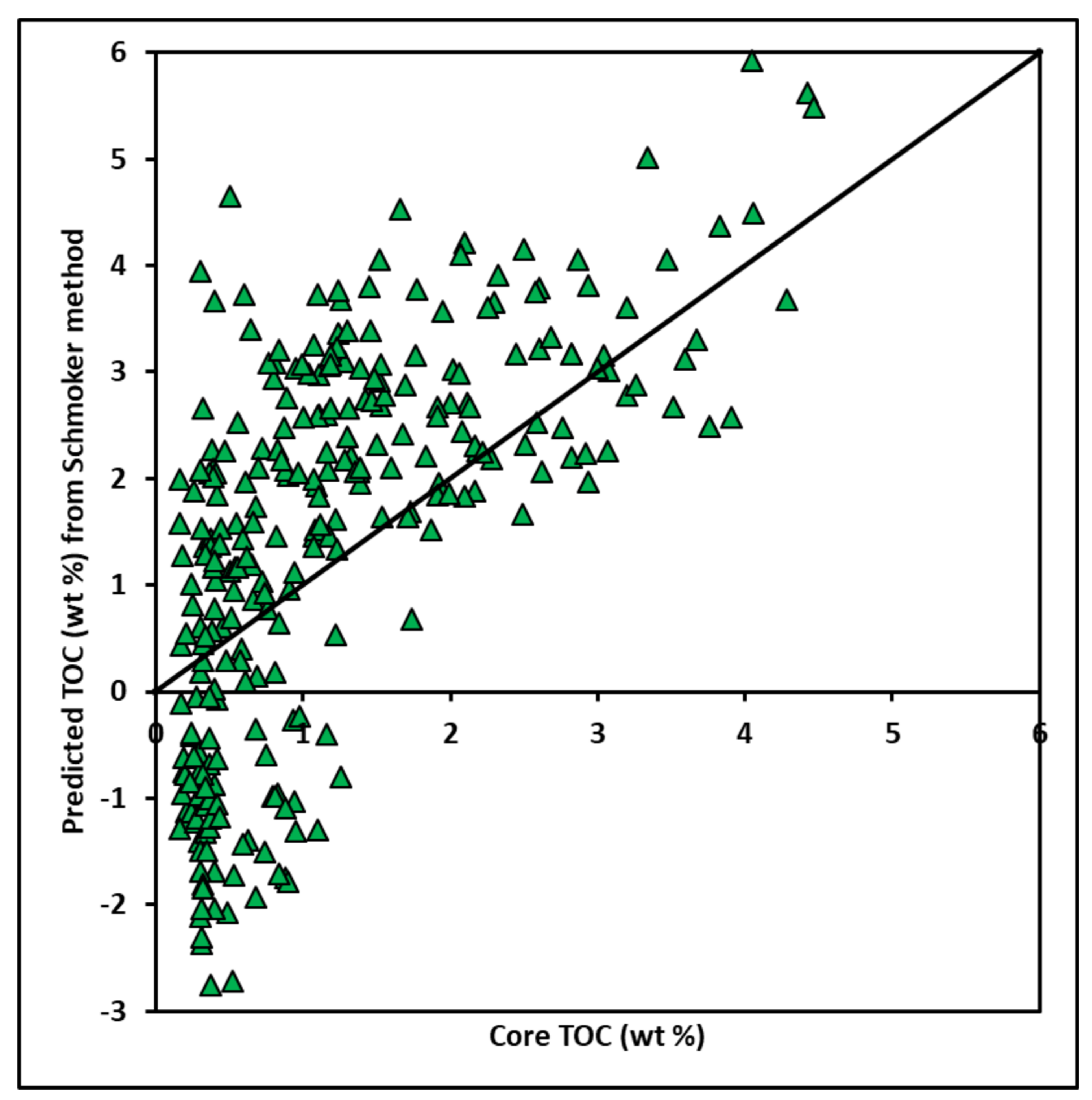
The Schmoker method, Equation (2) is used to calculate TOC of the Goldwyer formation of the Canning Basin. Correlation of predicted and core derived TOC is plotted in Figure 11. The estimated TOC differed significantly from the core TOC. Therefore, such an empirical method may not be suitable for this formation. Possibly, the amount of organic richness in the formation is not captured by the RHOB log. Moreover, there is limited scope left to adjust empirical constant (“a” and “b”) between core TOC and RHOB because of their poor correlation.
5.3.2. TOC Estimation with Passey Method
Passey’s method [26] is routinely applied for TOC computation in an unconventional shale reservoir. The method requires deep resistivity and sonic log. Another requisite of the method is LOM, which can be obtained from maturity information like vitrinite reflectance (R0) or Tmax data. Description of the baseline value of resistivity and compressional sonic travel time, vitrinite reflectance (R0), and LOM of all ten wells are in Table 7 (R0 information accumulated from various sources—Lukman pre-thesis, 2019; DMIRS database, 2019). LOM is computed from a third order polynomial function between R0 and LOM [10] as expressed by Equation (8) below
where LOM and R0 refers to is level of organic metamorphism and vitrinite reflectance (wt %), respectively.
An average value of LOM and R0 varies from 9.6 to 11.4 and from 0.75 to 1.1 wt %, respectively. The cross-plot of core TOC and TOC from Passey’s method in Figure 12 shows slightly better accuracy with a mean square error value of 0.694 relative to Schmoker’s method.
5.4. TOC Prediction with Ensemble Learning
The following five well-logs, namely, GR, DT, log10_LLD, RHOB, and NPHI, are used along with one additional feature, ΔlogR for predicting continuous TOC profile with supervised machine learning regression techniques. We checked the reliability of the feature weight factor by cross-plotting core TOC with each log response (Figure 13). Two input data groups are created based on observation of the above cross-plot analysis in Figure 13 which are: (i) Group1—GR, DT, NPHI, RHOB, log10_LLD, and ΔlogR; (ii) Group2—GR, DT, RHOB, log10_LLD, and ΔlogR. One linear ML model and four non-parametric ensemble models are trained and validated with two input attribute groups in predicting continuous TOC by following the workflow in Figure 3 (Section 4). LOOCV cross-validation is implemented, and their performance is recorded on the validation set in Table 8.
MLR, MLP, RF, SVM, and GBR model have achieved prediction accuracy with prediction error of 0.21, 0.14, 0.13, 0.16, and 0.15, respectively, whereas R2 scores are 77%, 85%, 86%, 83%, and 85%, respectively, for group-2 attribute set (Figure 14). The result pointed out that each of the ensemble learning models has a similar estimation capacity, but not the same output. Hence, we define an aggregated regressor that combines the performance of four ensemble learning model and returns the average estimate. The average predictor model was validated on a blind test well (Figure 15). Cross-plot of core TOC is compared with average ensemble predictor TOC values in Figure 16.
6. Discussion
The Goldwyer formation of the Canning Basin is highly complex in nature, which can be inferred from the large variety of core TOC value ranges from 0.16 wt % to 4.47 wt % with standard deviation of 1 wt % (Table 3) and also from previous research publication on maturity index, lithology, and core description of the drilled wells [5,31,59]. Figure 17 displayed the core plugs extracted from a well in the Goldwyer formation where it is very clear that the depositional environment is changing rapidly from shallow to deeper section. Due to the absence of NPHI and RHOB log on three studied wells we could not complete basic petrophysical evaluation nor estimate traditional TOC using Schmoker’s method. At the same time, the ensemble learning method with two different attribute groups could not be performed because of the shortage of those logs in Edgar Range-1, Mclarty-1, and Matches Spring-1.
NPHI is responsive to the variation of lithology, compaction, and hydrocarbon effect in the sub-surface. GR, DT, and log10_LLD are the most effective log to reflect the above variation. Therefore, our methodology of synthetic NPHI from these three input logs has clear physical significance in a petrophysical point of view. It is very common to generate a synthetic density log from the check shot or velocity-density transform [39] function. Bailey and Henson [36] predicted shallow bulk density profile from Gardner’s locally calibrated transform function on the Canning Basin but the prediction quality varies a lot. Here, synthetic RHOB log with Gardner’s transform and ML predictive modelling are compared on three wells. Lithology-specific velocity-density functions are not implemented because of the complex depositional history of Goldwyer shale formation [5,59]. It seems that the locally calibrated Gardner transform function does not follow the density data trend and was largely under-predicted (R2 value of 0.40). This could be due to the variation in organic matter type and depositional environment, etc. [30,36]; however, the machine learning model’s prediction accuracy is meaningfully higher (R2 value of 0.90) than Gardner’s empirical formula. The poorer performance of the Gardner empirical transform defended our decision to consider the ML application. Non-linearity, higher dimension, and overlapping nature of input–output features are the main factors of the ML model’s success [22,47,61]. Therefore, the generation of NPHI and RHOB log with machine learning algorithms become effective in a highly variable depositional environment such as the Goldwyer formation. For both of their predictions, the random forest was the best estimator with the squared value of the correlation coefficient being 93% and 85%, respectively, on the validation data set. Synthetic log generation helped to increase more core TOC samples into our TOC database, which is an advantage for any machine learning prediction [53].
The formation’s complexity is responsive to poor correlation coefficients from traditional TOC techniques (Schmoker and Passey) with an R2 value of 0.43 and 0.44 [27]. Moreover, the MLR method, which builds TOC log with linear regression algorithm from wire-line logs can reach an average correlation of 0.77 on the studied wells, but it is difficult to generalize because of the difference in log response and proven non-linearity across the Goldwyer formation from previous work in the Canning Basin [28,31]. Due to the non-unique relationship of wire-line logs and core TOC (laterally as well as spatially) in shale gas reservoirs, data-driven techniques are more reliable to improve prediction not only in a well, but also across the reservoir interval. The authors in [22,23] applied a non-parametric single ML model to organic-rich North America’s Barnett shale (TOC value reaches a maximum value range from 10 to 15 wt %), whereas Yu et al., 2017, adopted the GPR ML model with different kernel functions on the organic-rich Ordos Basin and poorly distributed organic matter content of Goldwyer shale (TOC is confined within 0 to 2 wt %). So, it is not practicable to obtain a unique predictor with any of the single ML models on the randomly varying organic matter content of the Goldwyer shale formation covering low to moderate TOC ranges (See Table 3; Figure 14). At the same time, optimization of the input feature weighting factor is necessary and is dealt with two different attribute groups. The effective attribute selection is followed by several researchers in their ML application. In the final TOC model building stage, neutron porosity log (NPHI) was dropped due to its poor relationship with core TOC, and it did not improve the model’s performance in any way (Table 8). So, this justified the selection of group-2 attributes for building the final TOC model.
In a given scenario of different well-logs (such as basic conventional logs, geochemical logs, and ECS log), the ensemble learning method automatically chooses the relevant input features when building more decision trees to improve its prediction power. This makes the application easier in any geological environment. Because of the capacity of generalizability in prediction, ensemble learning is relevant in the heterogeneous Goldwyer formation (see Figure 17) to improve prediction power compared to any single ML model. Each of the ensemble learning models reveals similar prediction accuracy. Henceforth, an average regressor is our choice as the final predictor model, which combines four ensemble learning models. The advantage is such a model balances out the weakness of each equally well-performing individual model. After a hundred realizations, we can still predict TOC on the validation data set with the same value of error function relative to each ensemble learning model. This combined regressor model is able to capture heterogeneity and non-linear interactions between features better than a single ML model. It also handles smaller data set size, and under- and overfitting problem by combining many estimators compared to any single GPR, SVM, or ANN model. All the above points make the ensemble learning model a robust predictor compared to either empirical or multi-linear regression, as can be seen from Figure 15.
7. Conclusions
This study provides an efficient TOC estimation workflow from wire-line log responses through a robust ensemble learning approach. In this paper we have demonstrated the importance of missing data samples by generating synthetic NPHI and RHOB logs through supervised machine learning regressor model when performing unconventional prospect analysis to understand organic richness of the Goldwyer formation. The random forest model was the outperforming regressor model for synthetic NPHI and RHOB log generation compared to the other models and empirical approach. The continuous TOC log was built with the traditional Schmoker and Passey methods on all the studied wells using three log responses (RHOB, DT, and LLD). Comparison of Rock-Eval TOC with traditional methods showed poor correlation, whereas our newly developed ensemble learning application improved the correlation from 44% to 80%. The final prediction TOC model is the average predictor model, which is the aggregate of the four ensemble learning models. In complex Goldwyer unconventional shale formation, the average predictor model is the best solution relative to any empirical or single ML model to predict TOC.
Author Contributions
Conceptualization, P.P.M., R.R. and I.E.; methodology, P.P.M., and R.R.; software, P.P.M.; validation, P.P.M., R.R. and I.E.; formal analysis, P.P.M.; investigation, P.P.M.; resources, R.R.; data curation, P.P.M.; writing—original draft preparation, P.P.M.; writing—review and editing, P.P.M., R.R. and I.E.; visualization, P.P.M.; supervision, R.R.; project administration, R.R. All authors have read and agreed to the published version of the manuscript.
Funding
This research received no external funding.
Institutional Review Board Statement
Not applicable.
Informed Consent Statement
Not applicable.
Acknowledgments
We gratefully acknowledge the Department of Mines, Industry Regulation, and Safety (DMIRS) of Western Australia for providing the data used in this study. We would also like to thank Vishal Das and Sumit Verma for their suggestions to improve the manuscript. We want to thank colleagues in the Unconventional Gas Research Group (UGRG) of Curtin University for their valuable inputs. PPM is financially supported by the Australian Government’s Research Training Program (RTP) scholarship, Curtin University’s Completion scholarship, and publication grant, PESA’s post-graduate scholarship, and AAPG’s Grants-in-Aid for providing financial support to complete his research study. We thank three anonymous reviewers to make the manuscript concise for a smooth review process.
Conflicts of Interest
The authors declare no conflict of interest.
Abbreviations
| Acronyms: | |
| AI | Artificial Intelligence |
| ML | Machine learning |
| GR | Gamma ray |
| LLD | Deep resistivity |
| DT | Compressional sonic travel time |
| NPHI | Neutron porosity |
| RHOB | Bulk density |
| ANN | Artificial neural network |
| MLR | Multi linear regression |
| MLP | Multi-layer perceptron |
| SVM | Support vector machine |
| RF | Random Forest |
| GBR | Gradient boosting regressor |
| TOC | Total organic carbon |
| LOM | Level of metamorphism |
| LOOCV | Leave-one-out cross-validation |
| GPR | Gaussian process regressor |
| MSE | Mean-squared error |
| Symbols: | |
| R0 | Vitrinite reflectance |
| R | Deep resistivity log |
| Δt | Compressional sonic travel time |
| Tmax | Maximum hydrocarbon generation temperature |
| Vp | Compressional wave velocity |
| ρb | Bulk density |
| wt % | Weight percentage |
| log10 | Logarithmic base 10 |
| R2 | Squared of correlation coefficient |
| ΔlogR | Separation of compressional sonic travel time and deep resistivity log |
Appendix A. Overview of Ensemble Learning Models Applied in This Study
Appendix A.1. Multi Linear Regression (MLR)
Linear regression is the most widely used technique in building a relationship between a dependent (output/target) and independent (input) variable. It uses a linear approach to model the correlation function between the input and output variables (Emelyanova et al., 2016). In the case of one input variable, it is known as single linear regression, whereas for multiple input variables, it is called multiple linear regression. The expression between input (xi) and output (yi) assuming a linear relation can be written as
In matrix notation Equation (A1) can be expressed as
where Y is a vector of observed values yi of the variable known as the output or dependent variable, X is the vector form of input or independent variables xi, θ is the (n + 1) dimensional parameter vector—elements are known as regression coefficient (for example, θ0 is intercept) and ε is vector form of the error term εi.
The aim is to minimize error of the cost-function (most used function is mean squared error function) which is defined as
where is the cost-function; y^i and yi represent the predicted and actual output.
Various parameter estimation techniques are available for linear regression. For example, least-squares methods, maximum-likelihood methods, etc. In the artificial intelligence domain, for example, machine learning, linear regression plays a crucial role and is the most fundamental supervised machine-learning algorithms. It is because of the algorithm’s simplicity and model interpretability. We have adopted a penalized least-square regression with an added regularization term (Lasso—L1-norm penalty with a penalty value of 0.01). This approach is useful to tackle the least-square method’s low bias and high variance consideration [35]. It is always a consistent approach to start building any regression model by including MLR to justify the necessity of complex model generation.
Appendix A.2. Multi-Layer Perceptron (MLP)
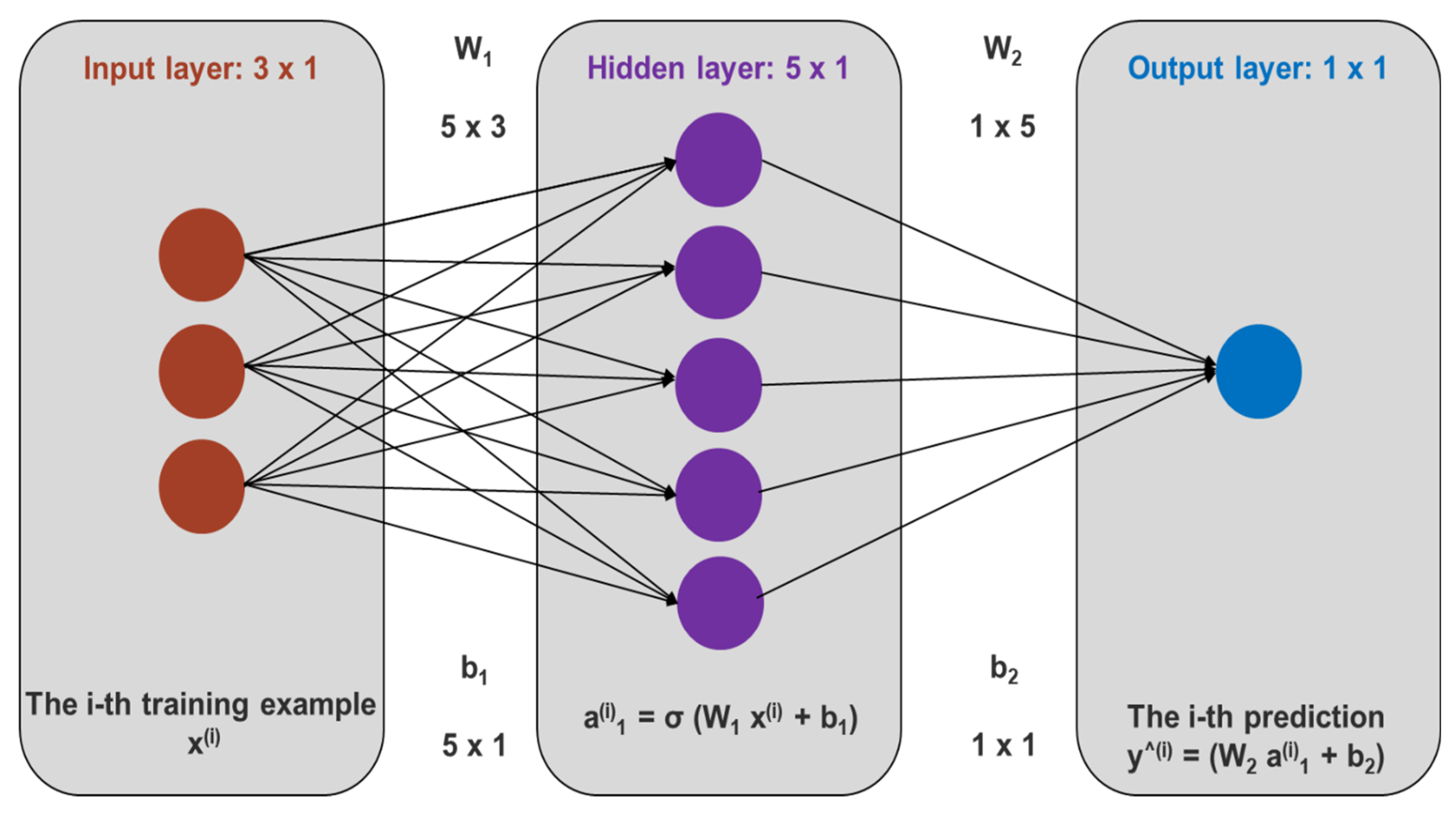
An artificial neural network is a computer algorithm that tries to mimic the human brain [27,61]. A neural network contains three or more layers: an input layer, one or more hidden layers, and an output layer. A neuron can pick an input vector x and computes its scalar with an adjustable weight vector W and produces an output vector y utilizing the non-linear activation function. The activation function, for example, sigmoid, aka logistic function in the demonstrated example in Figure A1, always restricts output between 0 and 1. Other activation functions can be used like rectified linear unit (RELU), exponential linear unit (ELU), and hyperbolic tangent (tanh) (e.g., personal communication Montaron, 2019). The algorithm runs through a forward propagation by outputting target values from known inputs, randomly chosen weights and then calculating the error between estimated and actual target values. This error is back propagated through the network to refine the weights of each neuron. Prior to running any experiment, the hyper-parameters are tuned (number of iterations, number of neurons, damping factor, etc.) by performing sensitivity analysis on training and validation data sets. In this study, an ensemble of MLPs is generated by different realizations and their predictions are integrated into a single solution by bootstrap aggregation (e.g., an average of multiple outputs). The tuned hyperparameters used in the present application are in Table A1.
Figure A1.
Schematic diagram of neural network architecture combining input layer, hidden layer, and output layer. In the figure x, y, W, b, and sigma are representing input vector, output vector, weighting vector, bias unit, and activation function respectively.
Figure A1.
Schematic diagram of neural network architecture combining input layer, hidden layer, and output layer. In the figure x, y, W, b, and sigma are representing input vector, output vector, weighting vector, bias unit, and activation function respectively.


Table A1.
Description of final optimized hyperparameters for artificial neural network ensemble.
| Neural Network Parameters (MLP) | Values |
|---|---|
| Number of inputs | 5 |
| Number of Outputs | 1 |
| Number of Neurons | 10 |
| Training algorithm | LBFGS |
| Alpha | 1 |
| Activation function | RELU |
| Maximum number of iterations | 2000 |
Appendix A.3. Support Vector Machine (SVM)
A support vector machine builds a set of hyperplanes in a high or infinite dimensional space which can be effectively applied for regression and classification tasks. Maximal margin hyperplane is the natural choice between input and output [23,42]. The best advantage of this method is providing a unique solution but could be more time consuming compared with other ML methods. In Figure A2, the concept of hyperplane is demonstrated by the visual display. An ensemble of kernel functions (e.g., exponential (RBF), Cauchy and Gaussian) and model parameters were analyzed using the grid-search approach for model tuning. The hyperparameters of the tuned model are provided in Table A2 below.
Figure A2.
Support vector machine schematic showing the maximal hyperplane design to predict the best hyperplane to perform the regression.
Figure A2.
Support vector machine schematic showing the maximal hyperplane design to predict the best hyperplane to perform the regression.

Table A2.
Final optimized hyperparameters for support vector machine ensemble modelling.
| Support Vector Machine Parameters | Values |
|---|---|
| Kernel | Cauchy |
| Penalty parameter C | 1 |
| Gamma | 1 |
Appendix A.4. Random Forest (RF)
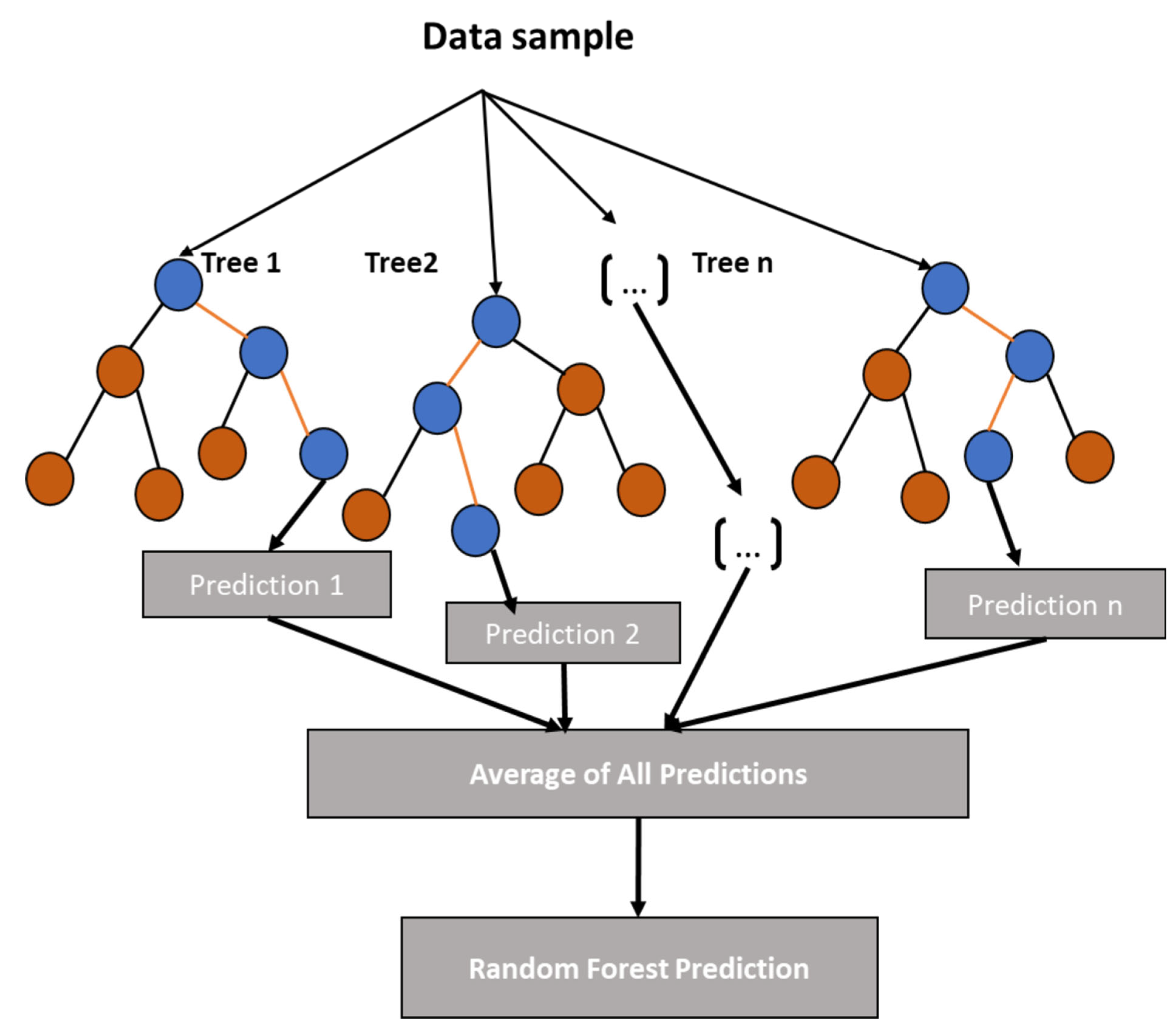
Random Forest is another ensemble learning method where the purpose is to combine the prediction of several base estimators with a given learning algorithm to improve the robustness of the prediction capability. It is one of the most successful non-parametric supervised machine learning models for regression and classification [35]. Among the two groups of ensemble methods, such as averaging and boosting method, random forest falls under the averaging group. The algorithm consists of many decision trees from a randomized variant of the tree induction algorithm [32]. It injects randomness into the training phase by bootstrapping (subsampling with replacement) and taking a different subset of features to split at each tree node. The insertion of randomness helps to tackle the variance of the estimator and handing of the overfitting problems compared to other methods. We created several estimators independently and finally averaged their predictions (see in Figure A3 for example). The two most important parameters that are adjusted (scikit-learn ensemble methods, [33]) are a number of trees and size of the random subset of features before producing the output. The RF parameters optimized in this study are presented in Table A3.
Figure A3.
Random Forest schematic showing, an ensemble of decision tree predictor and the average prediction defines the final output model.
Figure A3.
Random Forest schematic showing, an ensemble of decision tree predictor and the average prediction defines the final output model.

Table A3.
Description of final optimized parameters for random forest ensemble learning.
| Random Forest Parameters | Values |
|---|---|
| Number of trees | 200 |
| Maximum depth | 10 |
| Number of features | auto |
Appendix A.5. Gradient Boosting (GB)
Gradient boosting is an ensemble learning method under the boosting category where base estimators are generated in a sequential approach and at the same time reduce the bias of the estimator. It works on the principle of a combination of several weak models to produce a powerful predictor [62]. The process does not require any scaling of features and can easily capture non-linearities and feature interactions. The algorithm is applicable for both regression and classification problems. A few of the advantages of this process are the handling of heterogeneous features, robustness to outliers, and sequential predictor. However, the algorithm can cause overfitting during model validation and testing.
Gradient boosting trains a sequence of decision trees to obtain a minimum value of the loss function. The approach is followed by building a model from the training data set and then producing another model that tries to reduce the error from the first model. More models are added until the training data set is predicted near perfection. Model parameters are optimized in the boosting stage by the number of weak learners and the size of the tree. The optimized parameters of the gradient boosting regressor model are shown in Table A4.
Table A4.
Optimized hyperparameters of gradient boosting regression modelling.
| Gradient Boosting Regression Parameters | Values |
|---|---|
| Loss function | Least square |
| Number of boosting stages | 100 |
| Number of features | auto |
| Maximum depth | 2 |
References
- Dewhurst, D.N.; Sarout, J.; Delle Piane, C.; Siggins, A.F.; Raven, M.D. Empirical strength prediction for preserved shales. Mar. Pet. Geol. 2015, 67, 512–525. [Google Scholar] [CrossRef]
- Jarvie, D.M.; Hill, R.J.; Ruble, T.E.; Pollastro, R.M. Unconventional shale-gas systems the mississippian barnett shale of north-central texas as one model for thermogenic shale-gas assessment. AAPG Bull. 2007, 91, 475–499. [Google Scholar] [CrossRef]
- Rybacki, E.; Meier, T.; Dresen, G. What controls the mechanical properties of shale rocks?—Part Ii: Brittleness. J. Pet. Sci. Eng. 2015, 144, 39–58. [Google Scholar] [CrossRef] [Green Version]
- Das, B.; Chatterjee, R. Mapping of pore pressure, in-situ stress and brittleness in unconventional shale reservoir of krishna-godavari basin. J. Nat. Gas Sci. Eng. 2018, 50, 74–89. [Google Scholar] [CrossRef]
- Delle Piane, C.; Almqvist, B.S.; MacRae, C.M.; Torpy, A.; Mory, A.J.; Dewhurst, D.N. Texture and diagenesis of ordovician shale from the canning basin, western australia: Implications for elastic anisotropy and geomechanical properties. Mar. Pet. Geol. 2015, 59, 56–71. [Google Scholar] [CrossRef]
- Rezaee, R. (Ed.) Fundamentals of Gas Shale Reservoirs; Wiley: Hoboken, NJ, USA, 2015. [Google Scholar]
- Holt, R.M.; Fjær, E.; Stenebråten, J.F.; Nes, O.-M. Brittleness of shales: Relevance to borehole collapse and hydraulic fracturing. J. Pet. Sci. Eng. 2015, 131, 200–209. [Google Scholar] [CrossRef]
- Zoback, M.D.; Kohli, A.J. Unconventional Reservoir Geomechanics: Shale Gas, Tight Oil, and Induced Seismicity; Cambridge University Press: Cambridge, UK, 2019. [Google Scholar]
- Alshakhs, M. Shale Play Assessment of the Goldwyer Formation in the Canning Basin Using Property Modelling. Master’s Thesis, Curtin University, Perth, Australia, 2017. [Google Scholar]
- Alshakhs, M.; Rezaee, M.R. A new method to estimate total organic carbon (TOC) content, an example from goldwyer shale formation, the canning basin. Open Pet. Eng. J. 2017, 10, 118–133. [Google Scholar] [CrossRef] [Green Version]
- Yu, H.; Rezaee, R.; Wang, Z.; Han, T.; Zhang, Y.; Arif, M.; Johnson, L. A new method for toc estimation in tight shale gas reservoirs. Int. J. Coal Geol. 2017, 179, 269–277. [Google Scholar] [CrossRef] [Green Version]
- Holmes, M.; Holmes, A.; Holmes, D. A methodology using triple-combo well logs to quantify in-place hydrocarbon volumes for inorganic and organic elements in unconventional reservoirs, recognizing differing reservoir wetting characteristics—An example from the niobrara of the denver-julesburg basin, colorado. In Proceedings of the SPE/AAPG/SEG Unconventional Resources Technology Conference, Denver, CO, USA, 22–24 July 2019; Society of Exploration Geophysicists: Tulsa, OK, USA, 2019. [Google Scholar]
- Passey, Q.R.; Bohacs, K.M.; Esch, W.L.; Klimentidis, R.; Sinha, S. From oil-prone source rock to gas-producing shale reservoir—geologic and petrophysical characterization of unconventional shale gas reservoirs. In Proceedings of the International Oil and Gas Conference and Exhibition in China, Beijing, China, 8–10 June 2010; Society of Petroleum Engineers: Beijing, China, 2010. [Google Scholar]
- Yu, H.; Wang, Z.; Rezaee, R.; Zhang, Y.; Han, T.; Arif, M.; Johnson, L. Porosity estimation in kerogen-bearing shale gas reservoirs. J. Nat. Gas Sci. Eng. 2018, 52, 575–581. [Google Scholar] [CrossRef]
- Sone, H.; Zoback, M.D. Mechanical properties of shale-gas reservoir rocks—Part 1: Static and dynamic elastic properties and anisotropy. Geophysics 2013, 78, 381–392. [Google Scholar] [CrossRef] [Green Version]
- Sone, H.; Zoback, M.D. Mechanical properties of shale-gas reservoir rocks—Part 2: Ductile creep, brittle strength, and their relation to the elastic modulus. Geophysics 2013, 78, 393–402. [Google Scholar] [CrossRef]
- Vernik, L.; Liu, X. Velocity anisotropy in shales: A petrophysical study. Geophysics 1997, 62, 521–532. [Google Scholar] [CrossRef]
- Vernik, L.; Nur, A. Ultrasonic velocity and anisotropy of hydrocarbon source rocks. Geophysics 1992, 57, 727–735. [Google Scholar] [CrossRef]
- Wilczynski, P.M.; Domonik, A.; Lukaszewski, P. Anisotropy of strength and elastic properties of lower paleozoic shales from the Baltic Basin, Poland. Energies 2021, 14, 2995. [Google Scholar] [CrossRef]
- Iqbal, O.; Ahmad, M.; Abd Kadir, A. Effective evaluation of shale gas reservoirs by means of an integrated approach to petrophysics and geomechanics for the optimization of hydraulic fracturing: A case study of the Permian Roseneath and Murteree Shale Gas reservoirs, Cooper Basin, Australia. J. Nat. Gas Sci. Eng. 2018, 58, 34–58. [Google Scholar] [CrossRef]
- Jia, B.; Tsau, J.S.; Barati, R. A review of the current progress of CO2 injection EOR and carbon storage in shale oil reservoirs. Fuel 2019, 236, 404–427. [Google Scholar] [CrossRef]
- Verma, S.; Zhao, T.; Marfurt, K.J.; Devegowda, D. Estimation of total organic carbon and brittleness volume. Interpretation 2016, 4, T373–T385. [Google Scholar] [CrossRef] [Green Version]
- Zhao, T.; Verma, S.; Devegowda, D.; Jayaram, V. TOC estimation in the Barnett Shale from triple combo logs using support vector machine. In Proceedings of the 2015 SEG Annual Meeting, New Orleans, Louisiana, 18–23 October 2015; Society of Exploration Geophysicists: Tulsa, OK, USA, 2015. [Google Scholar]
- Schmoker, J.W. Determination of organic content of appalachian devonian shales from formation-density logs. Am. Assoc. Pet. Geol. Bull. 1979, 63, 1504–1509. [Google Scholar]
- Schmoker, J.W.; Hester, T.C. Organic carbon in bakken formation, united states portion of williston basin. Am. Assoc. Pet. Geol. Bull. 1983, 67, 2165–2174. [Google Scholar]
- Passey, Q.R.; Creaney, S.; Kulla, J.B.; Moretti, F.J.; Stroud, J.D. Practical model for organic richness from porosity and resistivity logs. AAPG Bull. 1990, 74, 1777–1794. [Google Scholar]
- Emelyanova, I.; Pervukhina, M.; Ben Clennell, M.; Dewhurst, D. Applications of standard and advanced statistical methods to Toc estimation in the mcarthur and georgina basins, Australia. Lead. Edge 2016, 35, 51–57. [Google Scholar] [CrossRef]
- Johnson, L.M.; Rezaee, R.; Kadkhodaie, A.; Smith, G.; Yu, H. Geochemical property modelling of a potential shale reservoir in the canning basin (western australia), using artificial neural networks and geostatistical tools. Comput. Geosci. 2018, 120, 73–81. [Google Scholar] [CrossRef]
- Ritzer, S.R.; Sperling, E.A. Characterizing the development of north american source rock reservoirs from the ordovician-jurassic: A proxy-based multivariate geochemical approach. In Proceedings of the 2019 AAPG Eastern Section Meeting: Energy from the Heartland, Columbus, OH, USA, 12–16 October 2019. [Google Scholar]
- Ghori, K.A.R.; Haines, P.W. Petroleum Geochemistry of the Canning Basin Western Australia: Basic Analytical Data 2004-05; Geological Survey of Western Australia: Perth, Australia, 2006. [Google Scholar]
- Triche, N.E.; Bahar, M. Shale gas volumetrics of unconventional resource plays in the canning basin, western Australia. In Proceedings of the SPE Unconventional Resources Conference and Exhibition-Asia Pacific, Brisbane, Australia, 11–13 November 2013; Society of Petroleum Engineers: Brisbane, Australia, 2013. [Google Scholar]
- Louppe, G. Understanding Random Forests. Ph.D. Thesis, University of Liege, Leige, Belgium, 2014. [Google Scholar]
- Pedregosa, F.; Varoquaux, G.; Gramfort, A.; Michel, V.; Thirion, B.; Grisel, O.; Blondel, M.; Prettenhofer, P.; Weiss, R.; Dubourg, V.; et al. Scikit-learn: Machine learning in python. J. Mach. Learn. Res. 2011, 12, 2825–2830. [Google Scholar]
- Emelyanova, I.; Pervukhina, M.; Clennell, M.B.; Dewhurst, D.N. Improving prediction of total organic carbon in prospective australian basins by employing machine learning. ASEG Ext. Abstr. 2016, 2016, 1–5. [Google Scholar] [CrossRef] [Green Version]
- Akinnikawe, O.; Lyne, S.; Roberts, J. Synthetic well log generation using machine learning techniques. In Proceedings of the SPE/AAPG/SEG Unconventional Resources Technology Conference, Houston, TX, USA, 23–25 July 2018; Society of Exploration Geophysicists, American Association of Petroleum Geologists, Society of Petroleum Engineers: Tulsa, OK, USA, 2018. [Google Scholar]
- Bailey, A.H.; Henson, P. Variation of vertical stress in the onshore canning basin, western Australia. APPEA J. 2019, 59, 364–382. [Google Scholar] [CrossRef]
- Gardner, G.H.F.; Gardner, L.W.; Gregory, A.R. Formation velocity and density—The diagnostic basics for stratigraphic traps. Geophysics 1974, 39, 770–780. [Google Scholar] [CrossRef] [Green Version]
- Mavko, G.; Mukerji, T.; Dvorkin, J. The Rock Physics Handbook: Tools for Seismic Analysis of Porous Media, 2nd ed.; Cambridge University Press: Cambridge, UK, 2009. [Google Scholar]
- Zoback, M.D. Reservoir Geomechanics; Cambridge University Press: Cambridge, UK, 2010. [Google Scholar]
- Castagna, J.P.; Batzle, M.L.; Eastwood, R.L. Relationships between compressional-wave and shear-wave velocities in clastic silicate rocks. Geophysics 1985, 50, 571–581. [Google Scholar] [CrossRef]
- Sondergeld, C.H.; Newsham, K.E.; Comisky, J.T.; Rice, M.C.; Rai, C.S. Petrophysical Considerations in Evaluating and Producing Shale Gas Resources. In Proceedings of the SPE Unconventional Gas Conference, Pittsburgh, PA, USA, 23 February 2010; Society of Petroleum Engineers: Pittsburgh, PA, USA, 2010. [Google Scholar]
- Andrew, N. Machine Learning. Coursera. Available online: https://www.coursera.org/learn/machine-learning (accessed on 1 March 2019).
- Lopes, R.; Jorge, A. Mind the gap: A well log data analysis. arXiv 2017, arXiv:1705.03669. [Google Scholar]
- Bhatt, A. Reservoir Properties from Well Logs Using Neural Networks. Ph.D. Thesis, Department of Petroleum Engineering and Applied Geophysics, Norwegian University of Science and Technology, Trondheim, Norway, 2002. [Google Scholar]
- Ghavami, F. Developing Synthetic Logs Using Artificial Neural Network: Application to Knox County in Kentucky. Master’s Thesis, West Virginia University, Morgantown, VA, USA, 2011. [Google Scholar]
- Dubois, M.K.; Bohling, G.C.; Chakrabarti, S. Comparison of Four approaches to a rock facies classification problem. Comput. Geosci. 2007, 33, 599–617. [Google Scholar] [CrossRef]
- Brendon, H. Facies classification using machine learning. Lead. Edge 2016, 35, 906–909. [Google Scholar]
- Elkatatny, S.; Tariq, Z.; Mahmoud, M.; Abdulraheem, A. New insights into porosity determination using artificial intelligence techniques for carbonate reservoirs. Petroleum 2018, 4, 408–418. [Google Scholar] [CrossRef]
- Wong, P.M.; Jian, F.X.; Taggart, I.J. A critical comparison of neural networks and discriminant analysis in lithofacies, porosity and permeability predictions. J. Pet. Geol. 1995, 18, 191–206. [Google Scholar] [CrossRef]
- Eshkalak, M.O.; Mohaghegh, S.D.; Esmaili, S. Synthetic, geomechanical logs for marcellus shale. In Proceedings of the SPE Digital Energy Conference, The Woodlands, TX, USA, 5 March 2013; Society of Petroleum Engineers: The Woodlands, TX, USA, 2013. [Google Scholar]
- Eshkalak, M.O.; Mohaghegh, S.D.; Esmaili, S. Geomechanical properties of unconventional shale reservoirs. J. Pet. Eng. 2014, 10, 961641. [Google Scholar] [CrossRef] [Green Version]
- Elkatatny, S.; Tariq, Z.; Mahmoud, M. Real time prediction of drilling fluid rheological properties using Artificial Neural Networks visible mathematical model (white box). J. Pet. Sci. Eng. 2016, 146, 1202–1210. [Google Scholar] [CrossRef]
- Mandal, P.P.; Rezaee, R. Facies classification with different machine learning algorithm—An efficient artificial intelligence technique for improved classification. ASEG Ext. Abstr. 2019, 2019, 1–6. [Google Scholar] [CrossRef] [Green Version]
- Polikar, R. Ensemble learning. In Ensemble Machine Learning; Zhang, C., Ma, Y., Eds.; Springer: Boston, MA, USA, 2012; pp. 1–34. [Google Scholar]
- Van Hattum, J.; Bond, A.; Jablonski, D.; Taylor-Walshe, R. Exploration of an unconventional petroleum resource through extensive core analysis and basin geology interpretation utilising play element methodology: The lower goldwyer formation, onshore canning basin, western Australia. APPEA J. 2019, 59, 464–481. [Google Scholar] [CrossRef]
- Ferguson, D.P. Petrophysical Considerations in Evaluating and Producing Shale Gas Resources. Master’s Thesis, University of Western Australia, Perth, Australia, 2016. [Google Scholar]
- Fortmann-Roe, S. Understanding the Bias-Variance Tradeoff. Available online: http://scott.fortmann-roe.com/docs/BiasVariance.html (accessed on 1 March 2020).
- Rokach, L. Ensemble methods in supervised learning. In Data Mining and Knowledge Discovery Handbook; Maimon, O., Rokach, L., Eds.; Springer: Boston, MA, USA, 2009; pp. 959–979. [Google Scholar]
- Testamanti, M.N. Assessment of Fluid Transport Mechanisms in Shale Gas Reservoirs. Ph.D. Thesis, Curtin University, Perth, Australia, 2019. [Google Scholar]
- Mandal, P.P. Integrated Geomechanical Characterization of Anisotropic Gas Shales: Field Appraisal, Laboratory Testing, Viscoelastic Modelling, and Hydraulic Fracture Simulation. Ph.D. Thesis, Curtin University, Perth, Australia, 2021. Unpublished. [Google Scholar]
- Graham, G. Neural networks. Lead. Edge 2018, 37, 616–619. [Google Scholar]
- Hastie, T.; Tibshirani, R.; Friedman, J. The Elements of Statistical Learning:Data Mining, Inference, and Prediction, 2nd ed.; Springer: Berlin/Heidelberg, Germany, 2009. [Google Scholar]
Figure 1.
(a) Location of the prospective Canning Basin along with its tectonic elements and proven major oil and gas occurrence. The main area of interest of unconventional shale reservoir is within the onshore Broome Platform are shown in red colors (modified from [55]). (b) Generalized stratigraphy map of Canning Basin where the study unit is highlighted by a black dotted rectangle in the Ordovician (modified from [56]).

Figure 2.
Workflow of a data-driven model for synthetic NPHI and RHOB log prediction with supervised ML regression algorithms. One linear and three non-linear ML algorithms are considered to choose the optimum prediction model.
Figure 2.
Workflow of a data-driven model for synthetic NPHI and RHOB log prediction with supervised ML regression algorithms. One linear and three non-linear ML algorithms are considered to choose the optimum prediction model.

Figure 3.
Workflow for TOC prediction with the ensemble learning approach. The process starts with the accumulation of input data sets and their QA/QC followed by ensemble learning implementation in several steps as shown by a red dotted arrow.
Figure 3.
Workflow for TOC prediction with the ensemble learning approach. The process starts with the accumulation of input data sets and their QA/QC followed by ensemble learning implementation in several steps as shown by a red dotted arrow.

Figure 4.
(a) Graphical illustration of bias and variance. The aim is to obtain a model that has low bias and low variance. (b) Contribution of bias and variance to the total error of the machine learning model (reproduced from the reference [57]). With increasing model complexity, error function reduced significantly for training data set but perform poorly in validation dataset, i.e., higher variance. The task to define a model in such a way that the bias and variance can tackle in validation and blind test data set.

Figure 5.
Variability reduction by application of three ensemble learning models (modified from [54]).
Figure 5.
Variability reduction by application of three ensemble learning models (modified from [54]).

Figure 6.
Leave-one-out cross-validation implementation procedure. n is the number of data sample, En is the MSE value of n times iteration of cross-validation. E is the summation over all n iterations MSE value.
Figure 6.
Leave-one-out cross-validation implementation procedure. n is the number of data sample, En is the MSE value of n times iteration of cross-validation. E is the summation over all n iterations MSE value.

Figure 7.
(a) Comparison of the original NPHI (green) and random forest predicted NPHI log (red) for three wells in the Goldwyer formation. Test well Looma-1 achieved a prediction accuracy with R2 value of 0.93. (b) Cross-plot of the original NPHI and estimated NPHI log using random forest predictor of the full data set. Linear regression trend line (yellow dotted line) shows R2 value of 0.96.

Figure 8.
Gardner’s [37] velocity-density transform plot of studied wells in the Goldwyer formation. The empirical trend does not fall on mean value (yellow triangle), and so, the curve is shifted to match (green trend line).
Figure 8.
Gardner’s [37] velocity-density transform plot of studied wells in the Goldwyer formation. The empirical trend does not fall on mean value (yellow triangle), and so, the curve is shifted to match (green trend line).

Figure 9.
Cross-plot of the measured bulk density and ML predicted density on the studied wells of the Goldwyer formation. The linear regression trend line (red) is overlaid on the plot. R2 value of 0.90 between measured and predicted density is achieved.
Figure 9.
Cross-plot of the measured bulk density and ML predicted density on the studied wells of the Goldwyer formation. The linear regression trend line (red) is overlaid on the plot. R2 value of 0.90 between measured and predicted density is achieved.

Figure 10.
Comparison of actual bulk density and random forest predicted bulk density log on three wells. Blind well Looma-1 is showing prediction accuracy index R2 of 0.84. The remaining two wells (Aquila-1 and Theia-1) are part of the training and validation data set. Predicted RHOB (red in color) are overlaid on the original RHOB log of Aquila-1 and Theia-1.

Figure 11.
Cross-plot of core TOC from Rock-Eval pyrolysis of core specimen and Schmoker’s method derive TOC. The black line is a 1:1 ratio between input and output variables. MSE and R2 values are 2.037 and 0.43, respectively.
Figure 11.
Cross-plot of core TOC from Rock-Eval pyrolysis of core specimen and Schmoker’s method derive TOC. The black line is a 1:1 ratio between input and output variables. MSE and R2 values are 2.037 and 0.43, respectively.

Figure 12.
Cross-plot of core TOC from Rock-Eval Pyrolysis and computed TOC from Passey method. The black line represents a 1:1 ratio between input and output variables. MSE and R2 values are 0.694 and 0.44, respectively.
Figure 12.
Cross-plot of core TOC from Rock-Eval Pyrolysis and computed TOC from Passey method. The black line represents a 1:1 ratio between input and output variables. MSE and R2 values are 0.694 and 0.44, respectively.

Figure 13.
Cross-plot of input features (petrophysical logs) and core TOC: (a) gamma-ray (GR), (b) logarithmic of deep resistivity (log10_LLD), (c) compressional sonic travel time (DT), (d) bulk density (RHOB), (e) neutron porosity (NPHI), and (f) separation of sonic and resistivity log (ΔlogR).
Figure 13.
Cross-plot of input features (petrophysical logs) and core TOC: (a) gamma-ray (GR), (b) logarithmic of deep resistivity (log10_LLD), (c) compressional sonic travel time (DT), (d) bulk density (RHOB), (e) neutron porosity (NPHI), and (f) separation of sonic and resistivity log (ΔlogR).

Figure 14.
MSE and R2 plot of one linear and four ensemble learning model for predictive TOC modelling. Four ensemble learning models have equally performed prediction outputs. The left y-axis scale presents MSE value whereas the right y-axis displays R2 score.
Figure 14.
MSE and R2 plot of one linear and four ensemble learning model for predictive TOC modelling. Four ensemble learning models have equally performed prediction outputs. The left y-axis scale presents MSE value whereas the right y-axis displays R2 score.

Figure 15.
Comparison of different TOC estimation methods on a test well of the Goldwyer shale formation. Track 1, 2, and 3 are showing GR, logarithmic of deep resistivity, and combination of RHOB and NPHI, respectively. The last four tracks present Schmoker, Passey, four ensemble learning models, and an aggregated ensemble model, estimating the TOC profiles, respectively. Core TOC (black triangle) is also overlaid on each of the last four tracks. In track 6, four ensemble model predicted TOC are compared, and there is significant variation of prediction capability along the well where the combination of four ensemble model in track 7 provides much better followed core TOC value.

Figure 16.
Cross-plot of core TOC and average ensemble predictor estimated TOC of all studied wells in the Goldwyer formation. The black line implies a 1:1 ratio. Prediction is not still perfect but improved significantly with R2 value of 0.86.
Figure 16.
Cross-plot of core TOC and average ensemble predictor estimated TOC of all studied wells in the Goldwyer formation. The black line implies a 1:1 ratio. Prediction is not still perfect but improved significantly with R2 value of 0.86.

Figure 17.
Core images from Theia-1 well at different depths in the Goldwyer formation of the Canning Basin. Sample depths are shown in GR log by a triangle. Lithological boundaries (black dashed line) are overlaid to show different Goldwyer units. Goldwyer-I and Goldwyer-III units are mostly clay-rich, whereas intermediate Goldwyer-II unit is a carbonate-rich interval. The first core example is mostly calcite rich mudstone and mostly homogeneous in Goldwyer-I unit. The second core image is a mixture of calcite and mudstone, and is highly heterogeneous. The third and fourth core are dark-grey color mudstone with lamination and highly complex composition of calcite and mudstone, respectively. The depth interval of third and fourth core sample is within 15 m, but a significant change in depositional environment is observed. The organic richness of these core samples varies from 0.04 to 2.25 wt % (from current ongoing research work of [60]).

Table 1.
The list of well log curves of the selected ten wells. Y indicates the log curve is present where N is non-existence of that curve. Edgar Range-1, Mclarty-1, and Matches Spring-1 do not have RHOB and NPHI curve.
Table 1.
The list of well log curves of the selected ten wells. Y indicates the log curve is present where N is non-existence of that curve. Edgar Range-1, Mclarty-1, and Matches Spring-1 do not have RHOB and NPHI curve.
| Available Well Log Curves | |||||
|---|---|---|---|---|---|
| Well | GR | DT | LLD | RHOB | NPHI |
| Edgar Range-1 | Y | Y | Y | N | N |
| Mclarty-1 | Y | Y | Y | N | N |
| Missing-1 | Y | Y | Y | Y | Y |
| Pictor East-1 | Y | Y | Y | Y | Y |
| Hilltop-1 | Y | Y | Y | Y | Y |
| Hedonia-1 | Y | Y | Y | Y | Y |
| Aquila-1 | Y | Y | Y | Y | Y |
| Canopus-1 | Y | Y | Y | Y | Y |
| Matches Spring-1 | Y | Y | Y | N | N |
| Theia-1 | Y | Y | Y | Y | Y |
Table 2.
Statistical description of input well log curves for synthetic NPHI and RHOB generation.
| GR | LLD | DT | |
|---|---|---|---|
| Unit | API | Ohm.m | us/ft |
| Data Count | 34,821 | 34,821 | 34,818 |
| Mean | 135.39 | 10.21 | 78.89 |
| Standard Dev. | 51.77 | 10.19 | 14.97 |
| Minimum | 21.50 | 0.46 | 17.19 |
| 25% | 95.38 | 4.07 | 66.97 |
| 50% | 134.91 | 7.30 | 77.10 |
| 75% | 177.88 | 12.49 | 89.47 |
| Maximum | 353.39 | 177.51 | 161.56 |
Table 3.
Complete statistical analysis of input and output variables for TOC predictive modelling exercise. ΔlogR is computed from Passey’s overlay technique [26] described in Section 2.1.
Table 3.
Complete statistical analysis of input and output variables for TOC predictive modelling exercise. ΔlogR is computed from Passey’s overlay technique [26] described in Section 2.1.
| GR | DT | RHOB | NPHI | log10_LLD | Core TOC | ΔlogR | |
|---|---|---|---|---|---|---|---|
| Unit | API | us/ft | g/cm3 | % | Ohm.m | wt % | Frac |
| Count | 283 | 283 | 283 | 283 | 283 | 283 | 283 |
| Mean | 145 | 83 | 2.63 | 20.25 | 0.93 | 1.20 | 0.42 |
| Standard Dev. | 36 | 12 | 0.08 | 7.70 | 0.32 | 1.00 | 0.37 |
| Minimum | 74 | 58 | 2.44 | 2.70 | 0.08 | 0.16 | −0.28 |
| Maximum | 235 | 108 | 2.83 | 43.02 | 1.74 | 4.47 | 1.46 |
Table 4.
Basic overview of all implemented algorithms where each of them are compared to understand their advantage and disadvantage (personal communication Irina Emelyanova, 2020).
Table 4.
Basic overview of all implemented algorithms where each of them are compared to understand their advantage and disadvantage (personal communication Irina Emelyanova, 2020).
| Feature | MLRs | ANNs | SVMs | RFs | GBs |
|---|---|---|---|---|---|
| Black box | No | Yes | Yes | No | No |
| Data flexibility (different types) | Yes | Yes | No | Yes | Yes |
| Unique solution | Yes | No | Yes | No | No |
| Overfitting | Yes | Yes | No | No | No |
| Efficient training time | No | Yes | No | Yes | No |
| Performance | No | Yes | Yes | Yes | Yes |
Table 5.
Mean squared error (MSE) and R2 score of four ML models for synthetic NPHI prediction. RF model achieved the least MSE and highest R2 score on the validation data set highlighted in the table.
Table 5.
Mean squared error (MSE) and R2 score of four ML models for synthetic NPHI prediction. RF model achieved the least MSE and highest R2 score on the validation data set highlighted in the table.
| Model Description | Training MSE | Training R2 Score | Validation MSE | Validation R2 Score |
|---|---|---|---|---|
| Multi-linear Regression | 9.86 | 0.86 | 10.12 | 0.86 |
| Multi-layer perceptron | 6.34 | 0.92 | 6.85 | 0.91 |
| Support vector machine | 3.87 | 0.95 | 5.58 | 0.92 |
| Random forest | 1.80 | 0.98 | 4.61 * | 0.93 * |
*—The minimum MSE value and highest R2 score.
Table 6.
Model comparison for synthetic RHOB prediction with four supervised ML models. RF model reached the least MSE and highest R2 score on the validation data set highlighted in the table.
Table 6.
Model comparison for synthetic RHOB prediction with four supervised ML models. RF model reached the least MSE and highest R2 score on the validation data set highlighted in the table.
| Model Description | Training MSE | Training R2 Score | Validation MSE | Validation R2 Score |
|---|---|---|---|---|
| Multi-linear regression | 0.01 | 0.51 | 0.01 | 0.51 |
| Multi-layer perceptron | 0.00 | 0.72 | 0.00 | 0.71 |
| Support vector machine | 0.00 | 0.58 | 0.00 | 0.58 |
| Random forest | 0.00 | 0.94 | 0.00 * | 0.85 * |
*—The minimum MSE value and highest R2 score.
Table 7.
Vitrinite reflectance, LOM, resistivity, and compressional sonic travel time baseline value of each studied well in the Goldwyer formation of the Canning Basin.
Table 7.
Vitrinite reflectance, LOM, resistivity, and compressional sonic travel time baseline value of each studied well in the Goldwyer formation of the Canning Basin.
| Well | R0 Range | LOM Average | Rbaseline | Δtbaseline |
|---|---|---|---|---|
| Theia-1 | 1.05–1.15 | 11.4 | 1.5 | 84 |
| Mclarty-1 | 0.85–1.08 | 10.8 | 2.5 | 92 |
| Hilltop-1 | 0.68–0.77 | 10.0 | 4.5 | 103 |
| Aquila-1 | 0.74–0.83 | 9.8 | 4 | 95 |
| Canopus-1 | 0.9–1.1 | 11.0 | 2.8 | 92 |
| Matches spring-1 | 0.8–0.9 | 10.2 | 3.5 | 92 |
| Missing-1 | 0.8–1.2 | 10.9 | 2.5 | 88 |
| Hedonia-1 | 0.91–1.09 | 11.0 | 6 | 108 |
| Pictor East-1 | 0.9–1.1 | 11.0 | 3.5 | 92 |
| Edgar Range-1 | 0.7–0.8 | 9.6 | 3 | 95 |
Table 8.
Supervised ensemble learning model’s performance of two different attribute groups in Goldwyer formation for TOC prediction. Every model’s accuracy is represented by MSE and R2 on the validation data set.
Table 8.
Supervised ensemble learning model’s performance of two different attribute groups in Goldwyer formation for TOC prediction. Every model’s accuracy is represented by MSE and R2 on the validation data set.
| Attribute Group | Group-1 | Group-2 | ||
|---|---|---|---|---|
| Model Description | MSE | R2 Score | MSE | R2 Score |
| Multi-linear regression | 0.23 | 0.76 | 0.21 | 0.77 |
| Multi-layer perceptron | 0.160 | 0.84 | 0.142 | 0.857 |
| Random forest | 0.152 | 0.854 | 0.132 * | 0.862 * |
| Support vector machine | 0.165 | 0.821 | 0.164 | 0.835 |
| Gradient boosting regression | 0.168 | 0.841 | 0.145 | 0.855 |
*—The minimum MSE value and highest R2 score.
Publisher’s Note: MDPI stays neutral with regard to jurisdictional claims in published maps and institutional affiliations. |
© 2021 by the authors. Licensee MDPI, Basel, Switzerland. This article is an open access article distributed under the terms and conditions of the Creative Commons Attribution (CC BY) license (https://creativecommons.org/licenses/by/4.0/).
Share and Cite
MDPI and ACS Style
Mandal, P.P.; Rezaee, R.; Emelyanova, I. Ensemble Learning for Predicting TOC from Well-Logs of the Unconventional Goldwyer Shale. Energies 2022, 15, 216. https://0-doi-org.brum.beds.ac.uk/10.3390/en15010216
AMA Style
Mandal PP, Rezaee R, Emelyanova I. Ensemble Learning for Predicting TOC from Well-Logs of the Unconventional Goldwyer Shale. Energies. 2022; 15(1):216. https://0-doi-org.brum.beds.ac.uk/10.3390/en15010216
Chicago/Turabian StyleMandal, Partha Pratim, Reza Rezaee, and Irina Emelyanova. 2022. "Ensemble Learning for Predicting TOC from Well-Logs of the Unconventional Goldwyer Shale" Energies 15, no. 1: 216. https://0-doi-org.brum.beds.ac.uk/10.3390/en15010216
Note that from the first issue of 2016, this journal uses article numbers instead of page numbers. See further details here.