Interaction of Electron Beams and Polarized Radiation in a Two-Beam Free-Electron Laser

Abstract

Recent research has focused on shorter pulses, new spectral ranges, higher photon fluxes, and the production of photons with a variety of polarizations. A time-dependent three-dimensional free-electron laser oscillator code was developed for a two-beam free-electron laser system with an elliptically polarized undulator. Characteristics of the interaction of the electron beams and polarized radiation in the XUV region were studied using this code. The code utilized an optical field using the spectral method in the paraxial approximation by a fast Fourier transformation, a Gaussian modal expansion for the optical field, and Newton–Lorentz force equations for particle tracking. As the emittance was increased, the degrees of polarization of the single-beam system with an elliptically polarized undulator and the two-beam system with a planar undulator were decreased significantly compared to those of a two-beam system with an elliptically polarized undulator in the XUV regions. The radiation intensities, the evolutions of the radiation power for wavelength, and the time in the two-beam system were increased significantly compared to those of a single-beam system. The statistical simulation result for the distribution of the number of shots in the degrees of polarization in the two-beam system was much better than that of the case with the single-beam system.

1. Introduction

There exists a large variety of the free-electron lasers (FELs), ranging from long-wavelength oscillators to X-ray FELs [1]. Research on the collective instability [2], stability [3], and the 3D effects of a waveguide [4] in free-electron lasers has played an important role. In a SASE, due to the shot noise, the radiation is affected by relatively poor temporal coherence and fluctuations. Research on seeding for the production of high-power and short-wavelength radiation in free-electron lasers has not provided sufficiently successful results. Several studies have been trying to solve these problems [5,6,7,8]. As an alternative method, McNeil et al. [9] proposed a two-beam FEL model using a single pass. The model with two electron beams in the one-dimensional limit showed an improved output coherence. The fundamental resonance wavelength for the fast (higher-energy) beam was a harmonic resonance wavelength of the slow (lower-energy) beam in the two-beam system.

Recent research has focused on shorter pulses, new spectral ranges, higher photon fluxes [10,11,12,13,14], and the production of photons with a variety of polarizations. Short-wavelength pulses of ultra-short duration and high intensity generated by extreme ultraviolet (XUV) free-electron lasers (FELs) play an important roles new frontiers in atomic and molecular physics, non-linear spectroscopy, solid density plasma physics, photochemistry, and structural biology [15,16,17].

The elliptically polarized undulator against variable polarization types have advantages due to their flexibility, simplicity, and lower cost of construction. A new 3D time-dependent code with 3D effects such as emittance, energy spread, optical diffraction, and nonlinear phenomena has been required for research on the interaction between the beam and polarized radiation. Chuncheon City is specializing in the biomaterial convergence industry and healthcare industry. The need for research on the XUV region is emerging for interdisciplinary convergence research between universities and cities. Therefore, we intend to undertake a preliminary study on the interaction between the electron beam and polarized radiation based on the proposed FEL facility, which is to be operated in the XUV regions with an electron beam energy of 900 MeV and a radiation wavelength of 135.96 nm.

In this paper, a time-dependent 3D free-electron-laser oscillator code was developed in a two-beam free-electron-laser system with an elliptically polarization undulator. Characteristics regarding the interaction of electron beam and polarized radiation in the XUV region were studied using the developed code. The elliptically polarized undulator consisted of two flat-pole-face undulators that were oriented perpendicular to each other. However, the developed code can be flexibly applied to planar, elliptical, and helical undulators according to the user’s needs. The ratios of the derivative of the spot size and the spot size for the fundamental and higher-order modes were calculated to study the refraction effects by using the 3D time-dependent code. The degree of polarization of a two-beam system with an elliptically polarized undulator was performed in the XUV region with an energy of 900 MeV for the higher-energy beam and 520 MeV for the lower-energy beam, and a current of 3000 A for the higher-energy beam and 1000 A for the lower-energy beam. The optimized results were compared to those of a single-beam system with an elliptically polarized undulator and a two-beam system with a planar undulator. The distribution of the number of shots in the two-beam system was compared with that of the single-beam system. The evolution of the radiation intensity for the wavelength was performed using multi-particle and multi-pass simulations. The radiation power for time was also calculated in the two-beam oscillator system using a new three-dimensional FEL code that we developed.

2. Theory and Formulation

The APPLE-II [18,19] undulator design is configurable to produce any type of undulator field from linearly polarized through elliptic polarization to a helically polarized field. All other undulator modules serve to provide a sufficient bunching of the electron beam in the last stage. For simplification, all these modules can be realized as planar devices, although they might be slightly longer than helical devices. The electromagnetic field is described by a modal expansion, and Gaussian optical modes are used for free-space propagation. The Gauss–Hermite modes are used for simulation of planar undulators, while the Gauss–Laguerre modes are used in simulating the interaction with elliptical or helical undulators. In this case, the vector potential representation [20] may be written in the following form:

$$\begin{array}{cc}& \delta A\left(x,y,z,t\right)={\displaystyle {\displaystyle \sum }_{l=-\infty }^{\infty }}{\displaystyle {\displaystyle \sum }_{n=0}^{\infty }}{\displaystyle {\displaystyle \sum }_{h=1}^{\infty }}{e}_{l,n,h}\left(r\right)\{\delta A_{l,n,h}^{\left(1\right)}\left({\widehat{e}}_x\sin {\phi }_{l,h}\pm u_e{\widehat{e}}_y\cos {\phi }_{l,h}\right)\\ & +\delta A_{l,n,h}^{\left(2\right)}\left({\widehat{e}}_x\cos {\phi }_{l,h}\mp u_e{\widehat{e}}_y\sin {\phi }_{l,h}\right)\},\end{array}$$

(1)

where $l$ and $n$ indicate transverse mode numbers, and $h$ is the harmonic number.

$$e_{l,n,h}\left(r\right)=\exp \left(-\frac{r^2}{w_h^2}\right){\xi }^{\left|l\right|}{L}_n^{\left|l\right|}\left({\xi }^2\right),$$

(2)

where $L_n^l$ is the associated Laguerre polynomial and $\xi =\sqrt{2}r/w_h$.

$${\phi }_{l,h}=h\left(kz-\omega t\right)+l\theta +\frac{{\alpha }_h{r}^2}{w_h^2}$$

(3)

where $w_h$ is the spot size of the $h^{th}$ harmonic, and ${\alpha }_h$ is related to the curvature of the phase front.

The ellipticity,$u_e$, related to the phase shift is given by:

$$u_e=\left\{\begin{array}{cc}\frac{1-\cos \varphi }{1+\cos \varphi }& ;0\le \varphi \le \pi /2\\ \frac{1+\cos \varphi }{1-\cos \varphi }& ;\pi /2\le \varphi \le \pi \end{array}\right.$$

(4)

The elliptical polarized undulator consists of two flat-pole-face undulator that are oriented perpendicularly to each other. Freund et al. [21] have been working on producing variable polarization in FEL using the APPLE-II undulator. An analytic representation of the APPLE-II undulator model [22] is represented by:

$$\begin{array}{l}{B}_w\left(x\right)=\\ B_w\left(z\right)\left(\sin \left(k_{w}z+\varphi \right)-\frac{\cos \left(k_{w}z+\varphi \right)}{k_w·B_w\left(z\right)}\frac{d{B}_w\left(z\right)}{dz}\right){\widehat{e}}_x\cosh k_{w}x\\ +B_w\left(z\right)\left(\sin k_{w}z-\frac{\cos k_{w}z}{k_w·B_w\left(z\right)}\frac{d{B}_w\left(z\right)}{dz}\right){\widehat{e}}_y\cosh k_{w}y\\ +B_w\left(z\right){\widehat{e}}_z\sinh k_{w}y\left[\cos \left(k_{w}z+\varphi \right)+\cos k_{w}z\right]\end{array}$$

(5)

where $B_w\left(z\right)$ is represented in the following form for the systematic component and the random component:

$$B_w\left(z\right)=B_w^{\left(s\right)}\left(z\right)+\Delta B_w\left(z\right)$$

(6)

where the systematic component $B_w^{\left(s\right)}$ describes the adiabatic entry taper and the random component $\Delta B_w$ indicates a random number generator or the measured imperfections of the undulator magnet. The systematic amplitude variations for the tapering at the ends of each undulator segment are assumed to be as follows:

$$B_w^{\left(s\right)}\left(z\right)=\left\{\begin{array}{cc}{B}_w{\sin }^2\left(\frac{k_{w}z}{4N_w}\right),& 0\le z\le N_{tap}{\lambda }_w\\ B_w,& N_{tap}{\lambda }_w<z\end{array}\right.$$

(7)

where $B_w$ is the field amplitude in the uniform region and $N_{tap}$ is the number of undulator periods in the tapering region.

Maxwell’s equation is given by:

$$\left(\frac{{\partial }^2}{\partial {\mathrm{x}}^2}+\frac{{\partial }^2}{\partial {\mathrm{y}}^2}+\frac{{\partial }^2}{\partial {\mathrm{z}}^2}-\frac{1}{{\mathrm{c}}^2}\frac{{\partial }^2}{\partial {\mathrm{t}}^2}\right)\mathsf{\delta }A\left(\mathrm{x},\mathrm{y},\mathrm{z},\mathrm{t}\right)=-{\mathsf{\mu }}_0\left(J^s+J^f\right)$$

(8)

$$\begin{array}{l}{J}^i=-e{\displaystyle {\displaystyle \sum }_{j=1}^{N_e}}{v}_j^i\mathsf{\delta }\left(x-x_j^i\right)\mathsf{\delta }\left(y-y_j^i\right)\frac{\mathit{\delta }\left(t-{\tau }_j^i\right)}{\left|v{z}_j^i\right|}\\ =-e{\displaystyle {\displaystyle \sum }_{j=1}^{N_e}}{\gamma }_j^i{v}_j^i\mathsf{\delta }\left(x-x_j^i\right)\mathsf{\delta }\left(y-y_j^i\right)\frac{\mathit{\delta }\left(t-{\tau }_j^i\right)}{{\gamma }_j^i\left|v{z}_j^i\right|}\\ =-e{\displaystyle {\displaystyle \sum }_{j=1}^{N_e}}{u}_j^i\mathsf{\delta }\left(x-x_j^i\right)\mathsf{\delta }\left(y-y_j^i\right)\frac{\mathit{\delta }\left(t-{\tau }_j^i\right)}{\left|u{z}_j^i\right|}\begin{array}{ccc} & & i=s,f\end{array}\end{array}$$

(9)

where the symbols $s$ and $f$ indicate the slow beam (lower-energy beam) and the fast beam (higher-energy beam), respectively; ${\gamma }_j$ is the Lorentz factor of the $j^{th}$ electron; $u_j={\gamma }_j{v}_j$,$u{x}_j={\gamma }_{j}v{x}_j$, $u{y}_j={\gamma }_{j}v{y}_j$, and $u{z}_j={\gamma }_{j}v{z}_j$; ${\tau }_j$ is the time at which the $j^{th}$ electron reaches the axial position z; and $N_e$ is the total number of electrons.

To get $\delta a_{l,n,h}^{\left(1\right)}$, substitute Equation (1) into Equation (8), average over the period $2\pi /\omega$ after multiplying by $\left({\widehat{e}}_x\cos {\phi }_{l,h}-u_e{\widehat{e}}_y\sin {\phi }_{l,h}\right)$, and orthogonalize in x and y after multiplying by $e_{l,n,h}\left(r\right)$ using slowly varying envelope approximation. The left side of Equation (8) is summarized as follows:

$$\begin{array}{ll}\frac{1}{2ek}cm{\pi }^2\left(1+u_e{}^2\right)& [-2\left(1+2n+\left|l\right|\right)\delta a_{l,n,h}^{\left(2\right)}+4{\alpha }_h\left\{n\delta a_{l,n-1,h}^{\left(1\right)}-\left(1+n+\left|l\right|\right)\delta a_{l,n+1,h}^{\left(1\right)}\right\}-2n\delta a_{l,n-1,h}^{\left(2\right)}\\ & +6\left(1+n+\left|l\right|\right)\delta a_{l,n+1,h}^{\left(2\right)}+2{\alpha }_h^2\left\{-\left(1+2n+\left|l\right|\right)\delta a_{l,n,h}^{\left(2\right)}+n\delta a_{l,n-1,h}^{\left(2\right)}+\left(1+n+\left|l\right|\right)\delta a_{l,n+1,h}^{\left(2\right)}\right\}\\ & +2hk{w}_h\frac{d}{dz}\left(w_h\right)[\delta a_{l,n,h}^{\left(1\right)}-n\delta a_{l,n-1,h}^{\left(1\right)}+\left(1+n+\left|l\right|\right)\delta a_{l,n+1,h}^{\left(1\right)}\\ & -{\alpha }_h\left\{-\left(1+2n+\left|l\right|\right)\delta a_{l,n,h}^{\left(2\right)}+n\delta a_{l,n-1,h}^{\left(2\right)}+\left(1+n+\left|l\right|\right)\delta a_{l,n+1,h}^{\left(2\right)}\right\}]\\ & +hk{w}_h^2[2\frac{d}{dz}\left(\delta a_{l,n,h}^{\left(1\right)}\right)\\ & +\frac{d}{dz}\left({\alpha }_h\right)\left\{-\left(1+2n+\left|l\right|\right)\delta a_{l,n,h}^{\left(2\right)}+n\delta a_{l,n-1,h}^{\left(2\right)}+\left(1+n+\left|l\right|\right)\delta a_{l,n+1,h}^{\left(2\right)}\right\}]]\end{array}$$

(10)

The right side of Equation (8) is summarized as follows:

$$\begin{array}{c}{\mu }_{0}e{\displaystyle {\displaystyle \sum }_{j=1}^{N_e}}\frac{n!}{\left(n+\left|l\right|\right)!}\{\frac{e_{l,n,h}\left(x_j^s,y_j^s\right)}{\left|u{z}_j^s\right|}·\left[{\widehat{e}}_{x}u{x}_j^s\cos {\phi }_{l,h}\left(x_j^s,y_j^s,{\tau }_j^s\right)-u_e{\widehat{e}}_{y}u{y}_j^s\sin {\phi }_{l,h}\left(x_j^s,y_j^s,{\tau }_j^s\right)\right]+\frac{e_{l,n,h}\left(x_j^f,y_j^f\right)}{\left|u{z}_j^f\right|}\\ ·\left[{\widehat{e}}_{x}u{x}_j^f\cos {\phi }_{l,h}\left(x_j^f,y_j^f,{\tau }_j^f\right)-u_e{\widehat{e}}_{y}u{y}_j^f\sin {\phi }_{l,h}\left(x_j^f,y_j^f,{\tau }_j^f\right)\right]\}\end{array}$$

(11)

Then, the ordinary differential equations for $\delta a_{l,n,h}^{\left(1\right)}$ and $\delta a_{l,n,h}^{\left(2\right)}$ will be obtained:

$$\begin{array}{c}-\frac{1}{2ek}cm{\pi }^2\left(1+u_e{}^2\right)\{\left(1+2n+\left|l\right|\right)\delta a_{l,n,h}^{\left(2\right)}\left[2+2{\alpha }_h\left({\alpha }_h-hk{w}_h\frac{d}{dz}\left(w_h\right)\right)+hk{w}_h^2\frac{d}{dz}\left({\alpha }_h\right)\right]\\ -2hk{w}_h\frac{d}{dz}\left(\delta a_{l,n,h}^{\left(1\right)}·w_h\right)\}=s_{l,n,h}^{s,\left(1\right)}+s_{l,n,h}^{f,\left(1\right)}\end{array}$$

(12)

where:

$$s_{l,n,h}^{i,\left(1\right)}=-e{\mu }_0{\displaystyle \sum }_{j=1}^{N_e}\frac{n!}{\left(n+\left|l\right|\right)!}\frac{e_{l,n,h}\left(x_j^i,y_j^i\right)}{\left|u{z}_j^i\right|}·\left[{\widehat{e}}_{x}u{x}_j^i\cos {\phi }_{l,h}\left(x_j^i,y_j^i,{\tau }_j^i\right)-u_e{\widehat{e}}_{y}u{y}_j^i\sin {\phi }_{l,h}\left(x_j^i,y_j^i,{\tau }_j^i\right)\right]\begin{array}{ccc} & & i=s,f\end{array}$$

(13)

To get $\delta a_{l,n,h}^{\left(2\right)}$, substitute Equation (1) into Equation (8), average over the period $2\pi /\omega$ after multiplying by $\left({\widehat{e}}_x\sin {\phi }_{l,h}+u_e{\widehat{e}}_y\cos {\phi }_{l,h}\right)$, orthogonalize in x and y after multiplying by $e_{l,n,h}\left(r\right)$ using slowly varying envelope approximation, and assume that the direct mode–mode coupling terms can be neglected.

Then, the left side of Equation (8) is summarized as follows:

$$\begin{array}{ll}-\frac{1}{2ek}cm{\pi }^2& \left(1+u_e{}^2\right)\left\{hk{w}_h^2\right\{2\frac{d}{dz}\left(\delta a_{l,n,h}^{\left(2\right)}\right)\\ & -\frac{d}{dz}\left({\alpha }_h\right)\left[-\left(1+2n+\left|l\right|\right)\delta a_{l,n,h}^{\left(1\right)}+n\delta a_{l,n-1,h}^{\left(1\right)}+\left(1+n+\left|l\right|\right)\delta a_{l,n+1,h}^{\left(1\right)}\right]\}\\ & +2hk{w}_h\frac{d}{dz}\left(w_h\right)\{\delta a_{l,n,h}^{\left(2\right)}+{\alpha }_h\left(-\left(1+2n+\left|l\right|\right)\delta a_{l,n,h}^{\left(1\right)}+n\delta a_{l,n-1,h}^{\left(1\right)}+\left(1+n+\left|l\right|\right)\delta a_{l,n+1,h}^{\left(1\right)}\right)\\ & -n\delta a_{l,n-1,h}^{\left(2\right)}+\left(1+n+\left|l\right|\right)\delta a_{l,n+1,h}^{\left(2\right)}\}-2\{-\left(1+2n+\left|l\right|\right)\left(1+{\alpha }_h^2\right)\delta a_{l,n,h}^{\left(1\right)}\\ & +n\left(-1+{\alpha }_h^2\right)\delta a_{l,n-1,h}^{\left(1\right)}+\left(1+n+\left|l\right|\right)\left(3+{\alpha }_h^2\right)\delta a_{l,n+1,h}^{\left(1\right)}+2{\alpha }_h[-n\delta a_{l,n-1,h}^{\left(2\right)}\\ & +\left(1+n+\left|l\right|\right)\delta a_{l,n+1,h}^{\left(2\right)}]\}\}\end{array}$$

(14)

The right side of Equation (8) is also summarized as follows:

$$\begin{array}{c}{\mu }_{0}e{\displaystyle {\displaystyle \sum }_{j=1}^{N_e}}\frac{n!}{\left(n+\left|l\right|\right)!}\{\frac{e_{l,n,h}\left(x_j^s,y_j^s\right)}{\left|u{z}_j^s\right|}·\left[{\widehat{e}}_{x}u{x}_j^s\sin {\phi }_{l,h}\left(x_j^s,y_j^s,{\tau }_j^s\right)+u_e{\widehat{e}}_{y}u{y}_j^s\cos {\phi }_{l,h}\left(x_j^s,y_j^s,{\tau }_j^s\right)\right]+\frac{e_{l,n,h}\left(x_j^f,y_j^f\right)}{\left|u{z}_j^f\right|}\\ ·\left[{\widehat{e}}_{x}u{x}_j^f\sin {\phi }_{l,h}\left(x_j^f,y_j^f,{\tau }_j^f\right)+u_e{\widehat{e}}_{y}u{y}_j^f\cos {\phi }_{l,h}\left(x_j^f,y_j^f,{\tau }_j^f\right)\right]\}\end{array}$$

(15)

Then, the ordinary differential equations for $\delta a_{l,n,h}^{\left(1\right)}$ and $\delta a_{l,n,h}^{\left(2\right)}$ will be obtained as well:

$$\begin{array}{c}-\frac{1}{2ek}cm{\pi }^2\left(1+u_e{}^2\right)\{\left(1+2n+\left|l\right|\right)\delta a_{l,n,h}^{\left(1\right)}\left[2+2{\alpha }_h\left({\alpha }_h-hk{w}_h\frac{d}{dz}\left(w_h\right)\right)+hk{w}_h^2\frac{d}{dz}\left({\alpha }_h\right)\right]\\ +2hk{w}_h\frac{d}{dz}\left(\delta a_{l,n,h}^{\left(2\right)}·w_h\right)\}=s_{l,n,h}^{s,\left(2\right)}+s_{l,n,h}^{f,\left(2\right)}\end{array}$$

(16)

where:

$$s_{l,n,h}^{i,\left(2\right)}=-e{\mu }_0{\displaystyle \sum }_{j=1}^{N_e}\frac{n!}{\left(n+\left|l\right|\right)!}\frac{e_{l,n,h}\left(x_j^i,y_j^i\right)}{\left|u{z}_j^i\right|}·\left[{\widehat{e}}_{x}u{x}_j^i\sin {\phi }_{l,h}\left(x_j^i,y_j^i,{\tau }_j^i\right)+u_e{\widehat{e}}_{y}u{y}_j^i\cos {\phi }_{l,h}\left(x_j^i,y_j^i,{\tau }_j^i\right)\right]\begin{array}{ccc} & & i=s,f\end{array}$$

(17)

$$\delta a_{l,n,h}^{\left(i\right)}=e\delta A_{l,n,h}^{\left(i\right)}/m{c}^2 \left(i=1,2\right)$$

(18)

The Newton–Lorentz force equations for the particles are given by:

$$\begin{array}{c}{\mathrm{vz}}_{\mathrm{j}}^{\mathrm{i}}\frac{\mathrm{d}}{\mathrm{dz}}{\mathit{p}}_{\mathrm{j}}^{\mathrm{i}}\\ =\frac{{\mathrm{uz}}_{\mathrm{j}}^{\mathrm{i}}}{{\mathsf{\gamma }}_{\mathrm{j}}^{\mathrm{i}}}\frac{\mathrm{d}}{\mathrm{dz}}{\mathit{p}}_{\mathrm{j}}^{\mathrm{i}}\\ =-\mathrm{e}\mathsf{\delta }\mathit{E}-\mathrm{e}{v}_{\mathrm{j}}^{\mathrm{i}}\times \left({\mathit{B}}_{\mathrm{w}}+\mathsf{\delta }\mathit{B}\right)\\ =-\mathrm{e}\mathsf{\delta }\mathit{E}-\mathrm{e}\frac{{\mathit{u}}_{\mathrm{j}}^{\mathrm{i}}}{{\mathsf{\gamma }}_{\mathrm{j}}^{\mathrm{i}}}\times \left({\mathit{B}}_{\mathrm{w}}+\mathsf{\delta }\mathit{B}\right)\begin{array}{ccc} & & i=s,f\end{array}\end{array}$$

(19)

where $\mathsf{\delta }\mathit{E}$ and $\mathsf{\delta }\mathit{B}$ correspond to the electric and magnetic fields of the complete super-position of Gaussian modes, ${\mathit{p}}_j$ is the momentum of the $j^{th}$ electron, and ${\mathrm{B}}_w$is the magnetostatic fields.

In a time-dependent simulation, the radiation in the $i^{th}$ slice is replaced by:

$$\delta A_i\to \delta A_i-\left(\delta z/{\lambda }_w\right)\left(\lambda /c\Delta t\right)\times \left[\delta A_i-\delta A_{i-1}\right]$$

(20)

The Stokes parameters [23] on the transverse position are given by:

$$\begin{array}{c}{S}_0\left(x,y\right)={\left|E_H\left(x,y\right)\right|}^2+{\left|E_V\left(x,y\right)\right|}^2=I_{\left(0^{°}\right)}\left(x,y\right)+I_{\left({90}^{°}\right)}\left(x,y\right),\\ S_1\left(x,y\right)={\left|E_H\left(x,y\right)\right|}^2-{\left|E_V\left(x,y\right)\right|}^2=I_{\left(0^{°}\right)}\left(x,y\right)-I_{\left({90}^{°}\right)}\left(x,y\right),\\ S_2\left(x,y\right)=\Re \left(E_H\left(x,y\right)E_V\left(x,y\right)\right)=I_{\left({45}^{°}\right)}\left(x,y\right)-I_{\left({135}^{°}\right)}\left(x,y\right),\\ S_3\left(x,y\right)=\Im \left(E_H\left(x,y\right)E_V\left(x,y\right)\right)=I_{RH}\left(x,y\right)-I_{LH}\left(x,y\right)\end{array}$$

(21)

The local polarized fraction of the light represents the fractional intensity of the polarized component at each $x,y$ position as:

$$P\left(x,y\right)=\frac{\sqrt{S_1{\left(x,y\right)}^2+S_2{\left(x,y\right)}^2+S_3{\left(x,y\right)}^2}}{S_0\left(x,y\right)}$$

(22)

The local elliptically polarized fraction of the light and the local direction of the elliptically polarization vector can be defined as:

$$P_{lin}\left(x,y\right)=\frac{\sqrt{S_1{\left(x,y\right)}^2+S_2{\left(x,y\right)}^2}}{S_0\left(x,y\right)}$$

(23)

$$\psi \left(x,y\right)=\frac{1}{2}{\tan }^{-1}\left[\frac{S_2\left(x,y\right)}{S_1\left(x,y\right)}\right]$$

(24)

3. Numerical Simulations

The interaction of the beams and the polarized radiation was studied using the three-dimensional FEL code in the two-beam oscillator system. The 3D time-dependent code with an optical resonator was capable of the interaction between the electron beam and polarized radiation in an arbitrarily polarized undulator. This code also utilized an optical field using the spectral method in the paraxial approximation by a fast Fourier transformation, and included 3D effects such as emittance and optical diffraction. Gaussian-mode superposition for the optical fields and the direct integration of the Newton–Lorentz force equations for particle tracking were used, and several optical elements such as mirrors and lenses could be installed. Since the need for research on the XUV region for the biomaterial convergence and healthcare industry is emerging for interdisciplinary convergence research between universities and cities, we intended to study the interaction between the electron beam and the polarized radiation in the XUV region with an electron beam energy of 900 MeV and a radiation wavelength of 135.96 nm, according to the user’s request. Simulations were performed for XUV regions with an energy of 900 MeV for the higher-energy beam and 520 MeV for the lower-energy beam. A radiation wavelength of 135.96 nm, a current of 3000 A for the higher-energy beam and 1000 A for the lower-energy beam, a wiggler period of 0.04 m, and a field amplitude$\mathrm{of} 1.2$T for a particle number of 1000 and a pass number of 300 were used to study the interaction of the polarized radiation and the electron beam. A normalized emittance of ${\epsilon }_n=0.01 ~ 0.1 \mathrm{mm}·\mathrm{mrad}$, an energy spread of 0.1–0.5%, and a time window of 260 fs in order to allow for slippage were also used in the simulations.

The number of CELLs was 5, and the CELLs consisted of {QDH, ds1, undulator1, ds2, QF, ds3, undulator2, ds4, QDH}; QDH was the half of QD (defocusing quadrupole), QF was the focusing quadrupole, and ds was the drift space. The length of one undulator was 3.6 m, one CELL was 8.16 m, and the total length is 40.8 m. The differential equations for simulations were integrated simultaneously with the 3D Lorentz force equations for the two-beam oscillator system with the elliptically polarized undulator. The stable operation of the optical cavity required $\mathrm{f}=\frac{\mathrm{r}}{2}>L_c/4$ for the mirror focal length f, the cavity round trip length $L_c$, and the mirror’s radius of curvature of r.

The spot size variation was related to the refractive guiding of the signal that was calculated by the three-dimensional code that we developed. The ratios of the derivative of the spot size and the spot size for each higher-order mode of $\mathrm{h}$= 1, 3, and 5 for the slow (lower-energy beam) and fast (higher-energy beam) beam are shown in Figure 1. Each maximum value represents the fundamental and higher-order modes of h = 1, h = 3, and h = 5. The maximum values for a single beam and two beams were in the range of ${10}^{-7}$ to ${10}^{-4}$or less with respect to the total length in both cases. The ratios of the derivative of the spot size and the spot size for each higher-order mode in the two-beam system were less affected by refraction, and there was no difference compared to those of the single-beam system.

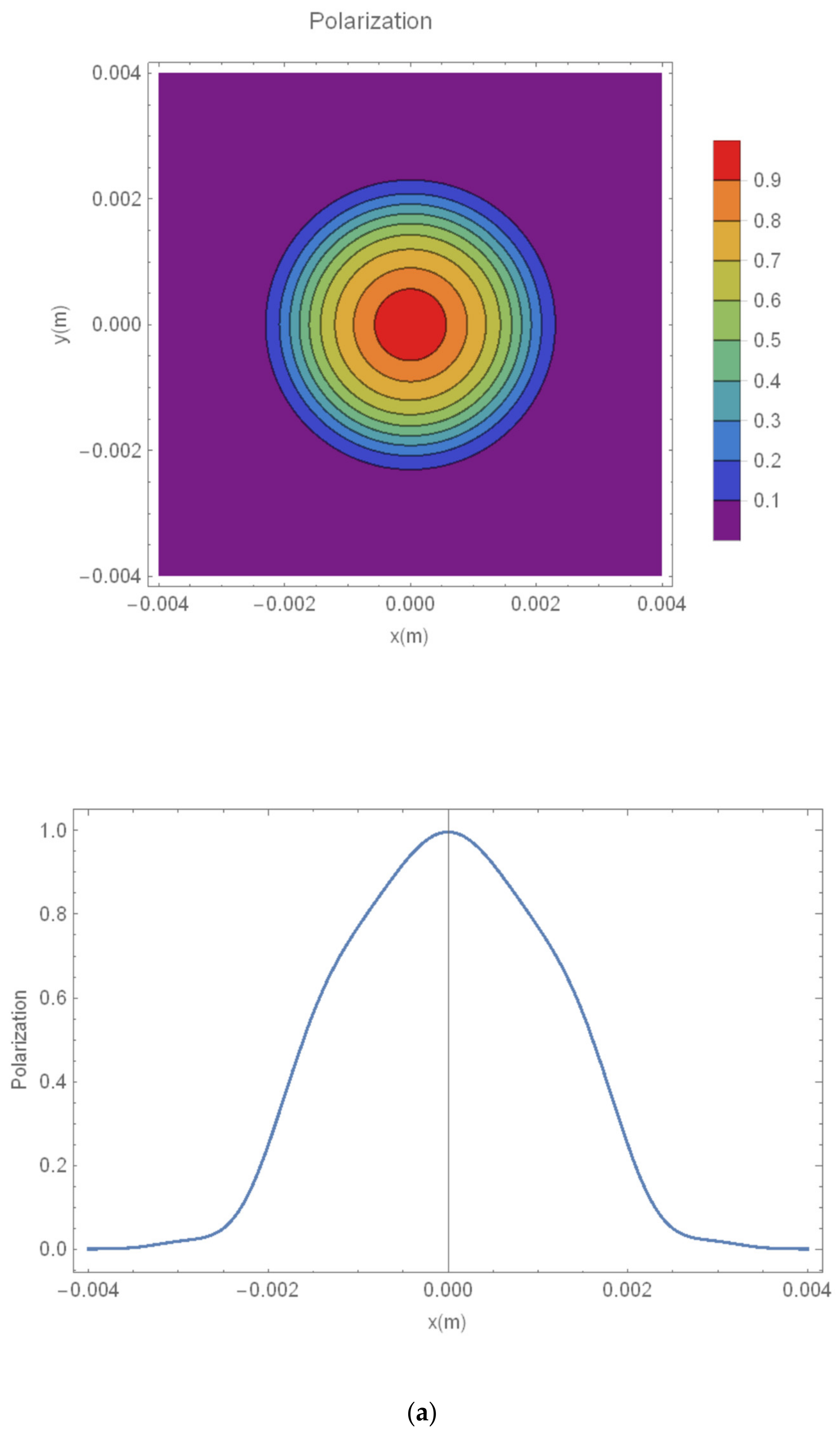
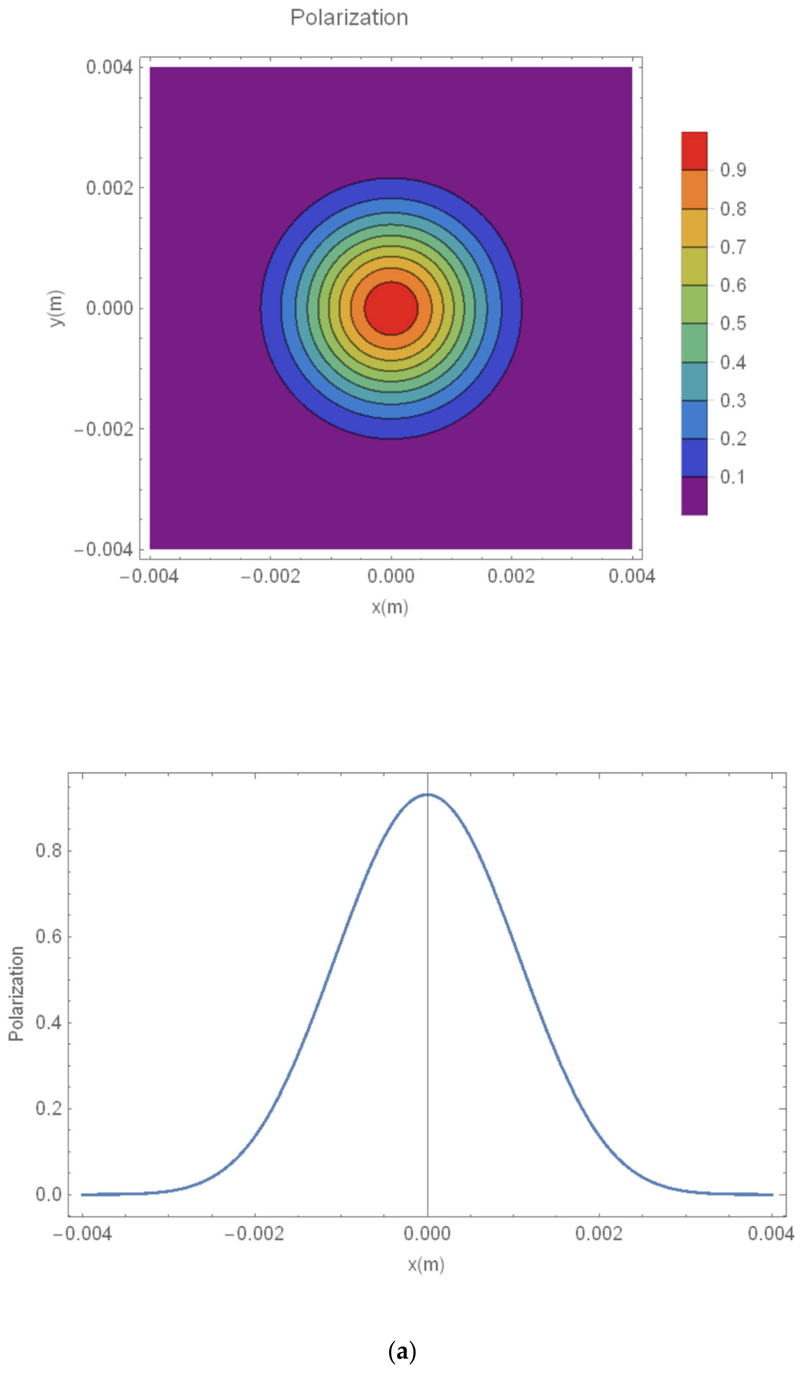
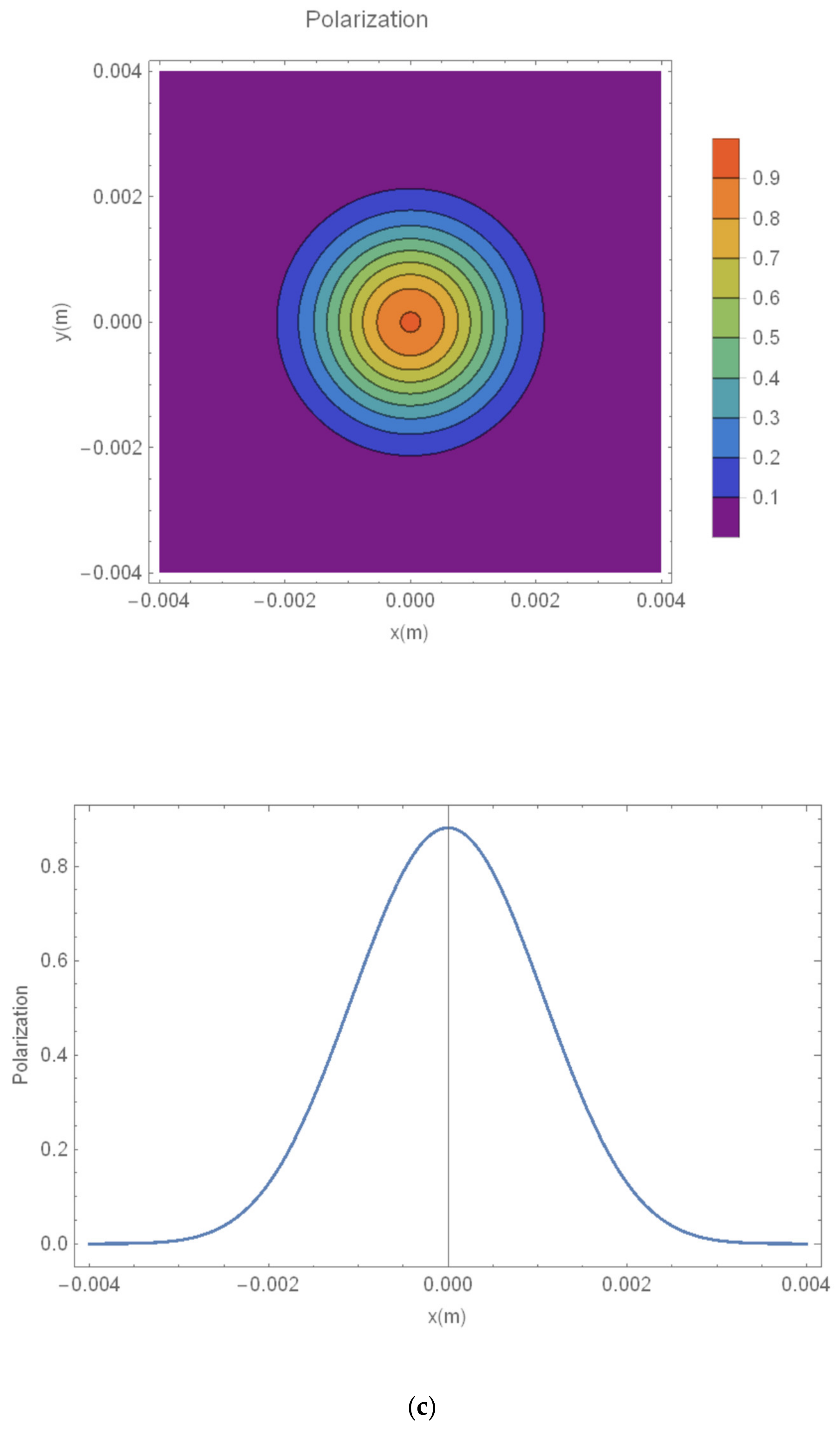
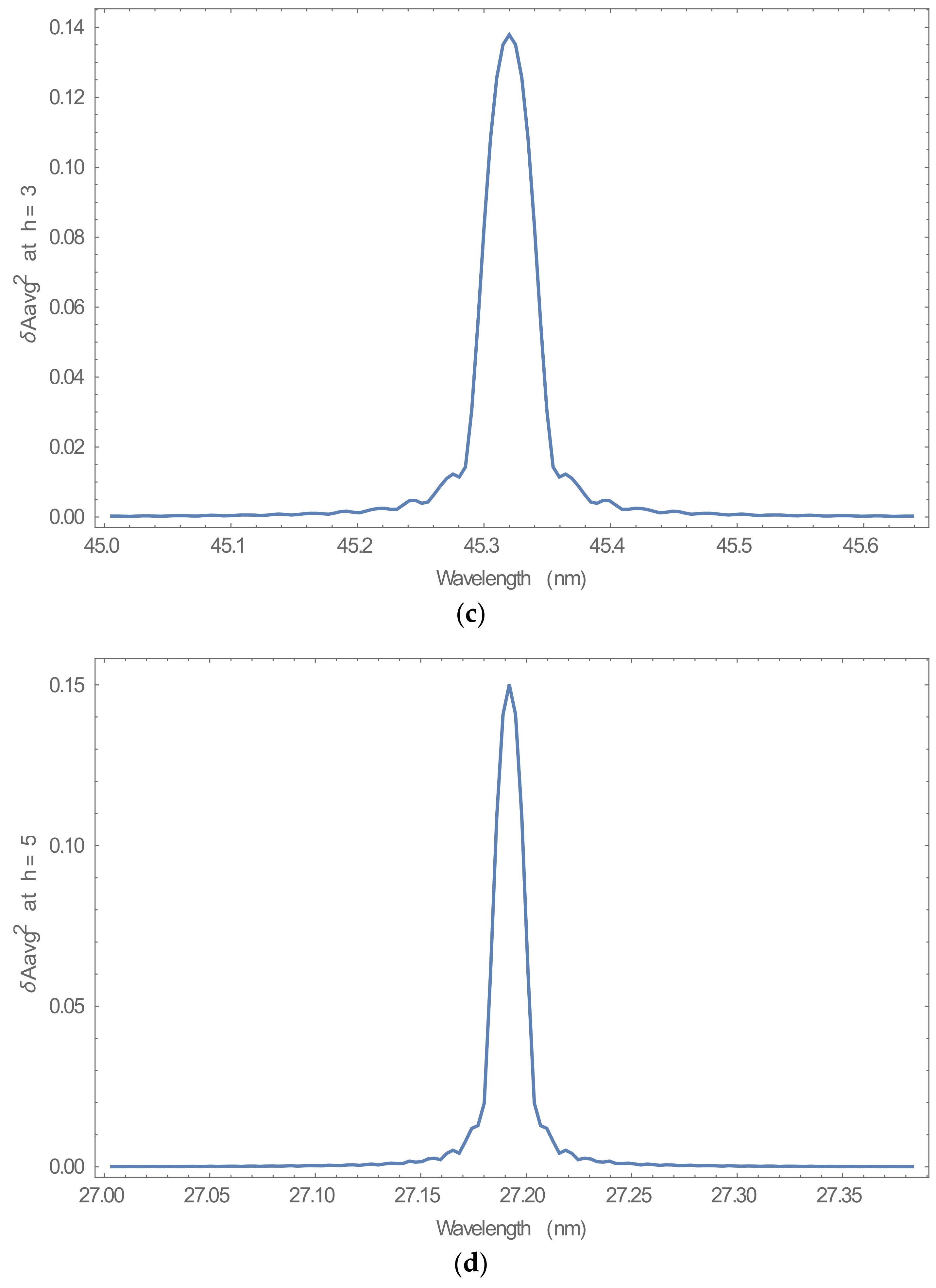
The Gauss–Laguerre modes were used in simulating the interaction of the beam and polarized radiation for the XUV regions. Our developed 3D time-dependent code treated the electromagnetic field as a superposition of the Gauss–Laguerre modes for three-dimensional representation with the transverse mode structure in the two-beam system and the single-beam system. The polarization and intensity of the XUV in the two-beam system with the elliptically polarized undulator were calculated for emittances of ${\epsilon }_n=0.01, 0.05, 0.1 \mathrm{mm}·\mathrm{mrad}$and an energy spread of 0.1%, as shown in Figure 2a–c. The results were compared to those of the planar undulator with an emittance of ${\epsilon }_n=0.05 \mathrm{mm}·\mathrm{mrad}$and an energy spread of 0.1%, as shown in Figure 2d.

The results were also compared with those of the single-beam system, as shown in Figure 3a–c. In the case of a degree of polarization over 90%, the degree of polarization in a two-beam system with an emittance of 0.05$\mathrm{mm}·\mathrm{mrad}$ was not significantly different from that of the case with an emittance of 0.01$\mathrm{mm}·\mathrm{mrad}$. However, the degree of polarization with an emittance of 0.1$\mathrm{mm}·\mathrm{mrad}$ was decreased by approximately 50% compared to the case with an emittance of 0.01$\mathrm{mm}·\mathrm{mrad}$. The degree of polarization in a single-beam system with an emittance of 0.1$\mathrm{mm}·\mathrm{mrad}$ was decreased by approximately 63% compared to the case with an emittance of 0.01 $\mathrm{mm}·\mathrm{mrad}$.

For the comparison of the degree of polarization of the two-beam system and the single-beam system, the degree of polarization in the two-beam system with an emittance of 0.01$\mathrm{mm}·\mathrm{mrad}$ was increased by approximately 27% compared to that of a single-beam system. However, the degree of polarization in a two-beam system with an emittance of 0.1$\mathrm{mm}·\mathrm{mrad}$ was increased by approximately 50% compared to that of a single-beam system. As the emittance increased, the degree of polarization of the single-beam system was decreased significantly compared to that of a two-beam system.

For the comparison of the degree of polarization with the elliptically polarized undulator and with the planar undulator, the degree of polarization of the two-beam system with the elliptically polarized undulator was increased by about 50% compared to the case with the planar undulator. However, the degree of polarization of the single-beam system with the elliptically polarization undulator was increased by about 30% compared to the case with the planar undulator.

The radiation intensity with the axial distance for the fundamental and higher-order modes of $\mathrm{h}$= 1, 3, and 5 modes in the two-beam system are shown in Figure 4. The evolution of the radiation field intensity was calculated for the fundamental mode of $\mathrm{l}=0, \mathrm{n}=0, \mathrm{and} \mathrm{h}=1$ in the two-beam oscillator system, as shown in Figure 4a. The result was compared to those of the higher-order modes of $\mathrm{l}=0, \mathrm{n}=0, \mathrm{h}=3 \mathrm{and} \mathrm{l}=0, \mathrm{n}=0,\mathrm{h}=5$ with an emittance of ${\epsilon }_n=0.1 \mathrm{mm}·\mathrm{mrad}$and energy spread of 0.1% in the two-beam system, as shown in Figure 4b,c, respectively.

Evolutions of the polarized radiation field intensity for the higher-order modes of $\mathrm{l}=0, \mathrm{n}=0 , \mathrm{h}=3 \mathrm{and} 5$ had lower radiation amplitudes than that of the fundamental mode of $\mathrm{l}=0, \mathrm{n}=0, \mathrm{and} \mathrm{h}=1$ in the two-beam oscillator system. For an emittance of ${\epsilon }_n=0.1 \mathrm{mm}·\mathrm{mrad}$and an energy spread of 0.1%$,$ the saturation intensities for the higher-order modes at 1000 particles and 300 passes were decreased by approximately 80% compared to that of the fundamental mode.

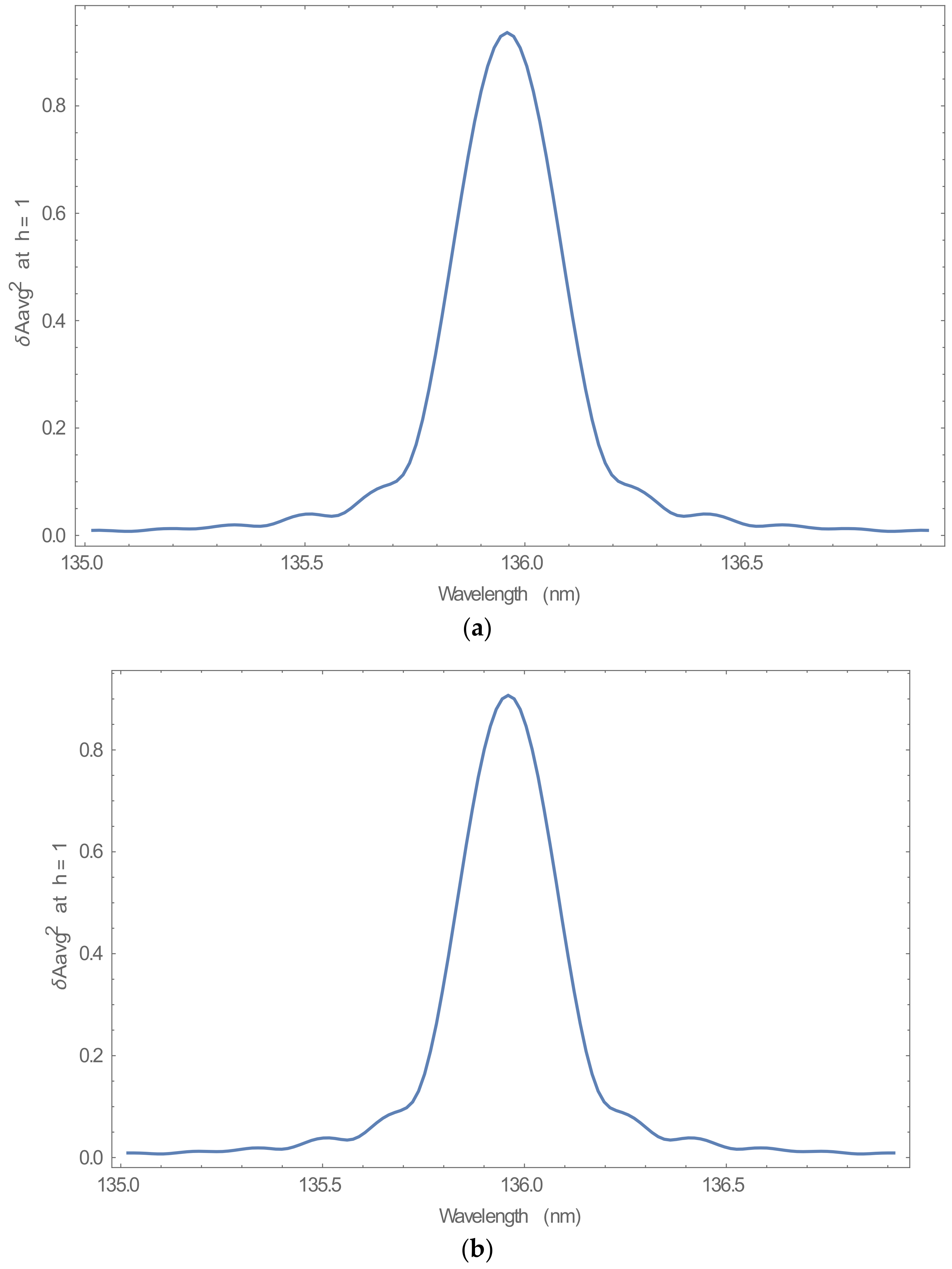
The evolution of the field intensity of the polarized radiation with axial distance for the fundamental mode of $\mathrm{l}=0, \mathrm{n}=0, \mathrm{and} \mathrm{h}=1$ was compared with those of a Genesis [24] simulation, as shown in Figure 5a,b, in the single-beam oscillator system. The harmonic field’s intensity of polarized radiation of the fundamental mode for this work showed a difference of approximately 3.3% compared to that obtained using the Genesis simulation in a single-beam configuration. The difference was due to the different formalism between our work with the higher-energy beam alone in the two-beam system and Genesis with a single-beam system, the number of grid points, and the mesh size, etc., in the simulations. The main difference was that the Genesis code used the wiggler-averaged-orbit approximation with a grid-based field solver. However, our code integrated the Newton–Lorentz equations with a Gaussian-mode superposition for the optical fields.

The results for the fundamental mode were compared to those of the higher-order modes of $\mathrm{l}=0, \mathrm{n}=0, \mathrm{h}=3 \mathrm{and} \mathrm{l}=0, \mathrm{n}=0,\mathrm{h}=5$ with an emittance of ${\epsilon }_n=0.1 \mathrm{mm}·\mathrm{mrad}$and energy spread of 0.1% in the single-beam system, as shown in Figure 5c,d.

However, the evolutions of the field intensity of polarized radiation for the higher-order modes of $\mathrm{l}=0, \mathrm{n}=0, \mathrm{h}=3 \mathrm{and} 5$ at 1000 particles and 300 passes were decreased significantly, by approximately 84% compared to that for the fundamental mode in the single-beam oscillator system.

The harmonic field’s intensity of polarized radiation of the fundamental mode in the two-beam system was increased by approximately 8% compared to that of the single-beam system.

The distributions of the number of shots for the polarized radiation are shown in Figure 6. The value for each quantity was obtained as an average over 28,000 shots with a bin width of 0.01. The maximum degree of polarization reached over 90%, which was concentrated at the center of the distribution of polarization. In the concentric distribution, the degree of polarization represented more than 90% based on 0.3, the degree of polarization represented over 60% for greater than 0.2 and less than 0.4, and the degree of polarization represented over 30% for greater than 0.1 and less than 0.5. The degree of polarization below 30% was ignored. The distribution of polarization in the two-beam system was concentrated in the center by more than approximately 7% compared to the single-beam system.

The evolution of the field intensity of polarized radiation for the radiation wavelength with axial distance for the fundamental and higher-order modes of $\mathrm{h}$= 1, 3, and 5 modes was calculated in the two-beam system with the elliptically polarized undulator, as shown in Figure 7. Evolution of the radiation field intensity versus the wavelength for the fundamental mode of $\mathrm{l}=0, \mathrm{n}=0, \mathrm{and} \mathrm{h}=1$ in the two-beam oscillator system is shown in Figure 7a. The results were compared to those of the higher-order modes of $\mathrm{l}=0, \mathrm{n}=0, \mathrm{h}=3 \mathrm{and} \mathrm{l}=0, \mathrm{n}=0,\mathrm{h}=5$ with an emittance of ${\epsilon }_n=0.1 \mathrm{mm}·\mathrm{mrad}$and an energy spread of 0.1% in the two-beam system, as shown in Figure 7b,c.

The evolution of the field intensity of polarized radiation for the wavelength for the higher-order modes of $\mathrm{l}=0, \mathrm{n}=0, \mathrm{h}=3 \mathrm{and} 5$ had lower radiation amplitudes than that of the fundamental mode in the two-beam oscillator system. It was found that the field intensity of polarized radiation for the wavelength had a maximum value when the resonant radiation wavelength was 135.96 nm. The radiation intensities for the higher-order modes at 1000 particles and 300 passes were decreased by approximately 80% relative to that for the fundamental mode.

The evolution of the field intensity of polarized radiation for the wavelength with axial distance for the fundamental and higher-order modes of $\mathrm{h}$= 1, 3, and 5 modes was calculated in the single-electron beam system, as shown in Figure 8.

The evolution of the field intensity of polarized radiation versus the wavelength for the fundamental mode of $\mathrm{l}=0, \mathrm{n}=0, \mathrm{and} \mathrm{h}=1$ is compared with that of the Genesis simulation in the single-beam oscillator system, as shown in Figure 8a,b. The harmonic field’s intensity between this work and the Genesis simulation showed a difference approximately 3.1% in the single-beam oscillator system. The radiation power versus time for the fundamental mode was also compared to the 4GLS XUV-FEL [25] with an energy of 950 MeV and a peak current of 1.5 kA, as shown in Figure 8e. The radiation power between this work (blue) and the 4GLS (red) showed a difference of approximately 4% in the single-beam oscillator system. The difference was due to the different formalism between our work with the higher-energy beam alone in the two-beam system and the Genesis simulation with a single-beam system, the number of grid points, and the mesh size, etc., in the simulations. The results for the fundamental mode were compared to those of the higher-order modes of $\mathrm{l}=0, \mathrm{n}=0, \mathrm{h}=3 \mathrm{and} \mathrm{l}=0, \mathrm{n}=0,\mathrm{h}=5$ with an emittance of ${\epsilon }_n=0.1 \mathrm{mm}·\mathrm{mrad}$and an energy spread of 0.1% in the single-beam system, as shown in Figure 8c,d. However, the evolution of the field intensity of polarized radiation for the wavelength for the higher-order modes of $\mathrm{l}=0, \mathrm{n}=0, \mathrm{h}=3 \mathrm{and} 5$ at 1000 particles and 300 passes was decreased significantly, by approximately 78% compared to that for the fundamental mode in the single-beam oscillator system. The normalized radiation field’s intensity of the fundamental mode for the wavelength in the single-beam system was decreased by approximately 5% compared to that of the two-beam system.

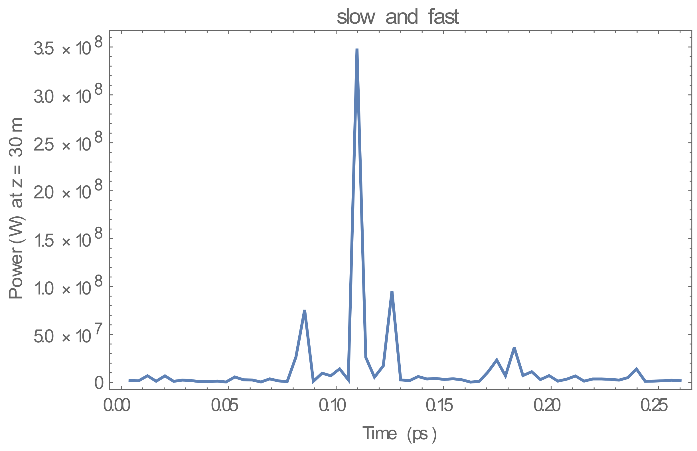
The power of polarized radiation versus time within the optical pulse are shown in Figure 9. The time window was 0.26 ps in order to allow for slippage across the electron bunch in the simulation The temporal pulse shape at z = 10.0 m for the sum of the fundamental and higher-order modes of h = 1, 3, and 5 in the two-beam system with the elliptically polarized undulator exhibited a broad distribution of spikes, and this corresponded to the development of temporal coherence, as shown in Figure 9. The evolution of temporal coherence is illustrated in Figure 9, Figure 10, Figure 11 and Figure 12. The temporal pulses are shown at z = 10.0 m, 20.0 m, 30.0 m, and 40.8 m, respectively. These figures correspond to the exponential gain region prior to saturation. It was clear that a large number of spikes coalesced into a smaller number of spikes. This phenomenon corresponded to the narrowing of the linewidth due to the development of coherence. The power at z = 40.8 m was increased by approximately 94% compared to that of z = 10.0 m.

4. Conclusions

The interaction of beams and polarized radiation in the XUV region in a two-beam system with an elliptically polarized undulator were studied using a time-dependent three-dimensional free-electron laser oscillator code that we developed. The ratios of the derivative of the spot size and the spot size for the fundamental and higher-order modes were calculated to study of the refraction effects using the 3D time-dependent simulations. The results for the two-beam system were less affected by refraction compared to those of the single-beam system. The two-beam oscillator system was less sensitive to the emittance and the energy spread. The degree of polarization of the two-beam system was much better than that of the single-beam system regarding the effect of the emittances, and the degree of polarization of the two-beam system was less sensitive to emittance compared to the single-beam system. As the emittance increased, the degree of polarization of the single-beam system was decreased significantly compared to that of the two-beam system. The distributions of the number of shots for the polarized radiation were performed for the statistical analysis. The distribution of polarization in the two-beam system was concentrated in the center, more than approximately 7% compared to the single-beam system. The degree of polarization of the two-beam system with the elliptically polarization undulator was much better than that of the case with the planar undulator. The radiation intensity of the high-energy beam alone in the two-beam system differed by less than about 4% compared to the Genesis simulation and the 4GLS radiation intensity in the single-beam system. The radiation intensity for the wavelength with two beams increased by about 8% compared to that of the single-beam system in the fundamental mode. The simulation results based on the emittance, the energy spread, and the higher-order modes were in good agreement with the Genesis simulation and the 4GLS radiation intensity in the single-beam system. The evolution of the radiation intensity for power versus time clearly showed that the early collection of a large number of spikes had coalesced into a smaller number of spikes. It was also clear that the temporal pulse shape was gradually narrowed and the power was increased due to the development of temporal coherence in the two-beam oscillator system with the elliptically polarized undulator.

References

- Freund, H.P.; Antonsen, T.M. Principles of Free-Electron Lasers; Chapman & Hall: London, UK, 1996; p. 162. [Google Scholar]
- Bonifacio, R.; Pelligrini, C.; Narducci, L.M. Collective instabilities and high-gain regime in a free electron laser. Opt. Commun. 1984, 118, 236. [Google Scholar]
- Nam, S.; Kim, K. Stability of an electron beam in a two-frequency wiggler with a self-generated field. J. Plasma Phys. 2010, 77, 257. [Google Scholar] [CrossRef]
- Nam, S.; Park, Y. Effects of waveguides on a free-electron laser with two electron beams. Laser Part. Beams 2019, 37, 386–391. [Google Scholar] [CrossRef]
- Bonifacio, R.; De Salvo Souza, L.; Pierini, P.; Scharlemann, E.T. Generation of harmonic radiation using the multi-cavity free-electron laser. Nucl. Instrum. Meth. Phys. Res. A 1990, 296, 787. [Google Scholar] [CrossRef]
- Yu, L.H.; Babzien, M.; Ben-Zvi, I.; DiMauro, L.F.; Doyuran, A.; Graves, W.; Johnson, E.; Krinsky, S.; Malone, R.; Pogorelsky, I.; et al. High-Gain Harmonic-Generation Free-Electron Laser. Science 2000, 289, 932–934. [Google Scholar] [CrossRef] [Green Version]
- Feldhaus, J.; Saldin, E.L.; Schneider, J.R.; Schneidmiller, E.A.; Yurkov, M.V. Possible application of X-ray optical elements for reducing the spectral bandwidth of an X-ray SASE FEL. Opt. Commun. 1997, 140, 341–352. [Google Scholar] [CrossRef] [Green Version]
- Faatz, B.; Feldhaus, J.; Krzywinski, J.; Saldin, E.L.; Schneidmiller, E.A.; Yurkov, M.V. Regenerative FEL amplifier at the TESLA test facility at DESY. Nucl. Instrum. Meth. Phys. Res. A 1999, 429, 424–428. [Google Scholar] [CrossRef]
- McNeil, B.W.J.; Robb, G.R.M.; Poole, M.W. Two-beam free electron laser. Phys. Rev. E 2004, 70, 035501. [Google Scholar] [CrossRef]
- Orfanos, I.; Makos, I.; Liontos, E.; Skantzakis, B.; Förg, D.; Charalambidis, D.; Tzallas, P. Attosecond pulse metrology. APL Photonics 2019, 4, 080901. [Google Scholar] [CrossRef] [Green Version]
- Frassetto, A.; Trabattoni, S.; Anumula, G.; Sansone, F.; Calegari, M.; Nisoli, M.; Poletto, L. High-throughput beamline for attosecond pulses based on toroidal mirrors with microfocusing capabilities. Rev. Sci. Instrum. 2014, 85, 103115. [Google Scholar] [CrossRef] [Green Version]
- Paola, F.; Hauke, H.; Enrico, A.; Callegari, C.; Capotondi, F.; Cinquegrana, P.; Giannessi, L. Pulse Duration of Seeded Free-Electron Lasers. Phys. Rev. X 2017, 7, 021043. [Google Scholar]
- Johnson, A.S.; Austin, D.R.; Wood, D.A.; Christian, B.; Andrew, G.; Konstantin, B.; Holzner, S.J. High-flux soft x-ray harmonic generation from ionization-shaped few-cycle laser pulses. Sci. Adv. 2018, 4, eaar3761. [Google Scholar] [CrossRef] [PubMed] [Green Version]
- Hort, O.; Dubrouil, A.; Khokhlova, M.A.; Descamps, D.; Petit, S.; Burgy, F.; Strelkov, V.V. High-order parametric generation of coherent XUV radiation. Opt. Express 2021, 29, 5982–5992. [Google Scholar] [CrossRef] [PubMed]
- Seddon, E.A.; Clarke, J.A.; Dunning, D.J.; Masciovecchio, C.; Milne, C.J.; Parmigiani, F.; Wurth, W. Short-wavelength free-electron laser sources and science: A review. Rep. Prog. Phys. 2017, 80, 115901. [Google Scholar] [CrossRef] [PubMed]
- Feldhaus, J.; Krikunova, M.; Meyer, M.; Möller, T.; Moshammer, R.; Rudenko, A.; Tschentscher, T.; Ullrich, J. AMO science at the FLASH and European XFEL free-electron laser facilities. J. Phys. B 2013, 46, 164002. [Google Scholar] [CrossRef]
- Miller, R.J.D. Femtosecond crystallography with ultrabright electrons and X-rays: Capturing chemistry in ac tion. Science 2014, 343, 1108–1116. [Google Scholar] [CrossRef]
- Bahrdt, J. Apple undulators for hghg-fels. In Proceedings of the FEL2006, Berlin, Germany, 27 August–1 September 2006; Bessy: Berlin, Germany, 2006. [Google Scholar]
- Bahrdt, J.; Frentrup, W.; Grimmer, S.; Kuhn, C.; Rethfeldt, C.; Scheer, M.; Schulz, B. Helmholtz-in-vacuum APPLE II undulator. In Proceedings of the 9th International Particle Accelerator Conference IPAC2018, Vancouver, BC, Canada, 29 April–4 May 2018. [Google Scholar]
- Campbell, L.T.; Freund, H.P.; Henderson1, J.R.; McNeil1, B.W.J.; Traczykowski1, P.; van der Slot, P.J.M. Analysis of ultra-short bunches in free-electron lasers. New J. Phys. 2020, 22, 073031. [Google Scholar] [CrossRef]
- Henderson, J.R.; Campbell, L.T.; Freund, H.P.; McNeil, B.W.J. Modelling elliptically polarized free electron lasers. New J. Phys. 2016, 18, 062003. [Google Scholar] [CrossRef]
- Freund, H.P.; van der Slot, P.J.M.; Grimminck, D.L.A.G.; Setija, I.D.; Falgari, P. Three-dimensional, time-dependent simulation of free-electron lasers with planar, helical and elliptical undulators. New J. Phys. 2017, 19, 023020. [Google Scholar] [CrossRef] [Green Version]
- Berry, H.G.; Gabrielse, G.; Livingston, A.E. Measurement of the Stokes parameters of light. Appl. Opt. 1977, 16, 3200. [Google Scholar] [CrossRef] [Green Version]
- Reiche, S. GENESIS 1.3: A fully 3D time-dependent FEL simulation code. Nucl. Instrum. Meth. Phys. Res. Sect. A 1999, 429, 243. [Google Scholar] [CrossRef]
- McNeil, B.W.J.; Robb, G.R.M.; Thompson, N.R.; Jones, J.; Poole, M.W. Design considerations for the 4gls xuv-fel. In Proceedings of the 27th International Free Electron Laser Conference, Stanford, CA, USA, 21–26 August 2005. [Google Scholar]
Figure 1.
The ratio of the derivative of the spot size and the spot size of two beams (a) and a single beam (b) for each higher-order mode of = 1, 3, and 5 modes.
Figure 2.
The degree of polarization of the radiation amplitude in the two-beam system with the transverse mode structure of the Gauss–Laguerre modes (color online): (a) an emittance of and an energy spread of 0.1%; (b) an emittance of and an energy spread of 0.1%; (c) an emittance of and an energy spread of 0.1%; (d) planar undulator with an emittance of and an energy spread of 0.1%.
Figure 3.
The degree of polarization of the radiation amplitude in the single-beam system with the transverse mode structure of the Gauss–Laguerre modes (color online): (a) an emittance of and an energy spread of 0.1%; (b) an emittance of and an energy spread of 0.1%; (c) an emittance of and an energy spread of 0.1%.
Figure 4.
Evolutions of the field intensity of polarized radiation for the fundamental and higher-order modes of (a), (b), and (c) in the two-beam system with an emittance of and an energy spread of 0.1% (color online).
Figure 5.
Evolutions of the field intensity of polarized radiation for the fundamental and higher-order modes of (a) h = 1 (Genesis simulation), (b) h = 1, (c) h = 3, and (d) h = 5 modes in the single-beam system with a fast beam for an emittance of and an energy spread of 0.1% (color online).
Figure 6.
The distribution of the number of shots in the two-beam system (a) and in the single-beam system (b). The polarization states reached the degree of polarization over 90% at the center of the distribution.