Integration of Electromagnetic Geophysics Forward Simulation in Coupled Flow and Geomechanics for Monitoring a Gas Hydrate Deposit Located in the Ulleung Basin, East Sea, Korea

Abstract

We investigate the feasibility of electromagnetic (EM) geophysics methods to detect the dissociation of gas hydrate specifically from a gas hydrate deposit located in the Ulleung Basin, East Sea, Korea via an integrated flow-geomechanics-EM geophysics simulation. To this end, coupled flow and geomechanics simulation is first performed with the multiple porosity model employed, where a mixed formulation with the finite volume (FV) and finite element (FE) methods are taken for the flow and geomechanics, respectively. From the saturation and porosity fields obtained from the coupled flow and geomechanics, the electrical conductivity model is established for the EM simulation. Solving the partial differential equation of electrical diffusion which is linearized using the 3D finite element method (FEM), the EM fields are then computed. For numerical experiments, particularly two approaches in the configuration for the EM methods are compared in this contribution: the surface-to-surface and the surface-to-borehole methods. When the surface-to-surface EM method is employed, the EM is found to be less sensitive, implying low detectability. Especially for the short term of production, the low detectability is attributed to the similarity of electrical resistivity between the dissociated gas (CH${}_4$) and hydrate as well as the specific dissociation pattern within the intercalated composites of the field. On the other hand, when the surface-to-borehole EM method is employed, its sensitivity to capture the produced gas flow is improved, confirming its detectability in monitoring gas flow. Hence, the EM geophysics simulation integrated with coupled flow and geomechanics can be a potential tool for monitoring gas hydrate deposits.

1. Introduction

Gas hydrates are one of the important future energy resources such that a vast amount of natural gas is trapped inside its specific structure and can be produced through its dissociation. Several methods to dissociate and produce gas from the hydrates were proposed in the literature and experiments including the depressurization and thermal stimulation [1,2]. Recently, various depressurization strategies have been investigated aiming at the improved geomechanical/wellbore stability while maintaining the productivity [3]. Because the hydrates are buried mostly in the unconsolidated sands distributed in the deep sea or permafrost regions over the globe, precise monitoring schemes for the gas hydrate deposits in terms of both the fluid flow and the geomechanical responses accompanied during the dissociation process cannot be stressed enough to enhance the productivity and safety.

For monitoring and characterizing the subsurface flow with more accuracy, the electromagnetic (EM) methods have recently been applied to geophysics and spotlighted [4,5]. Through the EM survey, it is known that the change of various physical quantities such as temperature and permittivity, i.e., electric polarizability, can potentially be detected through wave inversion or the joint inversion with the seismic data (i.e., spatio-temporal data inversion problem) and by generating electrical resistivity tomography (ERT) [6,7,8]. Particularly for the gas hydrate exploration, dense hydrates are found to have direct relations to the amount of electrical resistivity [9,10,11]. Moreover, the EM geophysical method has the potential to complement the (micro-)seismic methods to detect subsurface geometry or dynamics (e.g., fracture propagation) [12], because they are highly sensitive to fluids in pores and fractures and can provide independent information about fluid flow coupled with geomechanics [13,14].

The objective of this study is to investigate the feasibility of the EM method focusing on the detectability of the fluid flow, i.e., the flow of dissociated methane from the gas hydrate. To this end, we apply an integrated flow-geomechanics-EM geophysics simulation to a specific gas hydrate deposit, located near the site of UBGH2-6 in the Ulleung Basin, East Sea, Korea [3,15,16]. For coupled flow-geomechanical simulation first, depressurization induces the dissociation of hydrates, which results in the flow of fluids (gas and water) in the quasi-static state assumed. The multiple porosity (MP) model [3,17] is employed to reduce the high computational costs for the field-wide simulation, especially for the geomechanics calculation of a vertically heterogeneous deposit with a very thin and intercalated reservoir compared to the overburden. Several simulators exist for coupled flow and geomechanics simulation, especially for the gas hydrates which are either based on the kinetic and equilibrium model, such as MH21 [18], STOMP-HYD-KE [19], or TOUGH+HYDRATE [20]. In this study, we use T+M${}^{\mathrm{AM}}$, which is recently developed and validated with multiscale experiments [21]. The T+M${}^{\mathrm{AM}}$ simulator consists of TOUGH+HYDRATE and ROCMECH [22], which are flow and geomechanics simulators, respectively, for which a mixed formulation—the finite volume (FV) and finite element (FE) methods for fluid and geomechanics, respectively—is taken [23]. In addition, the exact formulation of axisymmetry using the cylindrical coordinate is applied for coupled flow and geomechanics to enhance the accuracy. For the two-way coupling of geomechanics and fluid with heat flow, we employ the fixed-stress sequential method [17,24] for the MP system, and the coupling between fluid flow and geomechanics can be rigorously performed. The porosity-dependent permeability model, based on a function of ice/hydrate saturation within pore space, is also applied.

Regarding the EM simulation that follows, we employ the diffusion model [14,25] to calculate the electric field. Hydrological and petrophysical parameters (i.e., change in saturations of fluids and in pore volume while gas is extracted from the hydrates) computed by the coupled flow-geomechanical simulation are first transformed into electrical conductivity via Archie’s law based on the rock physics model. With the results of electrical conductivity, the diffusive EM field is then obtained through the EM simulation. For the EM simulation, the 3D Cartesian domain is employed, which is converted from the 2D axisymmetric domain for coupled flow and geomechanics. Specifically, the 3D finite element method (FEM) [13,25,26,27] with the tetrahedral unstructured grids are used to accurately handle irregular gas hydrate plume not conforming to rectangular Cartesian grids. In this study, two configurations for the EM method are compared: the surface-to-surface and the surface-to-borehole methods. Numerical experiments with a series of time-lapsed data obtained from the 3D integrated flow-geomechanics-EM simulation then substantiate the feasibility of the EM method to detect the dissociation of gas hydrate, i.e., the gas flow. When the marine surface-to-surface EM method is employed, the EM is found to be less sensitive particularly for the short term of production, because of the specific dissociation pattern within the intercalated composites shown in the field as well as the similarity of electrical resistivity between dissociated methane (CH${}_4$) and hydrate. Meanwhile, the surface-to-borehole EM method is found to be more sensitive and can successfully be applied to detect the gas flow dissociated from hydrates.

This study demonstrates that we can simulate the gas production from the hydrate deposits in two separate spatial scales using the integrated flow-geomechanics-EM geophysics simulation. From coupled flow and geomechanics simulation, surface deformation and pressure can be highlighted, particularly such responses "around" the well [28,29], whereas through the EM method, we simulate EM fields over a larger volume of gas hydrate deposit to monitor reservoir-scale changes. These different length scales can be complementary to each other for more precise characterization of the gas flow. The proposed EM methods can also further be expanded in various forms to estimate the bulk amount of gas extraction/production from the gas hydrate deposits as well as evaluate any unfavorable potential leak of methane during production. It is a promising tool that can be applied to other subsurface flow monitoring (e.g., the CO${}_2$ geological storage [30,31]) with an appropriate rock physics model.

2. Mathematical Formulations

In this section, the mathematical formulations for the integrated flow-geomechanics-EM geophysics simulation are presented. In order to model the natural gas production from gas hydrate deposits via depressurization methodology, the governing equations for coupled flow and geomechanics are explained first in Section 2.1. In Section 2.2, we present the constitutive relations of the MP model employed in this study. Subsequently, the governing equation for EM geophysics and electrical conductivity model chosen for the study are explained in Section 2.3. Lastly, in Section 2.4, the dynamic permeability model relating to the dynamic porosity is briefly explained.

2.1. Governing Equations for Coupled Flow and Geomechanics

Gas hydrates can be dissociated via several methods, including representative thermal stimulation or depressurization. For example, the depressurization makes pressure drop below the equilibrium pressure curve, which can induce the hydrate dissociation. Meanwhile, the dilation of the geomaterials can be induced by thermal stimulation. With the direct thermal expansion, fluid pressure can be increased and the effective stress can be decreased. We rely on the poromechanics theory [32] for fully coupled flow and the geomechanics model to precisely compute and characterize the production and response of gas hydrate deposits.

Governing equation for geomechanics is based on the momentum balance following the quasi-static assumption,

$$\mathbf{Div}\sigma +{\rho }_b\mathit{g}=\mathbf{0},$$

(1)

where ${\rho }_b$ is the bulk density, $\sigma$ is the total stress tensor, and $\mathit{g}$ is the gravity vector. Note that Div is the divergence operator. The small strain theory and infinitesimal transformation allow us to obtain the engineering strain tensor $\epsilon$, i.e., the symmetric gradient of the displacement vector $\mathit{u}$,

$$\epsilon =\frac{1}{2}(\mathbf{Grad}\mathit{u}+{\left(\mathbf{Grad}\mathit{u}\right)}^T),$$

(2)

where Grad is the gradient operator and T is the transpose operator.

Meanwhile, the fluid flow has its governing equation from the mass balance [20]:

$$\frac{d}{dt}{\int }_{\Omega }{m}^{k}d\Omega +{\int }_{\Gamma }{\mathit{f}}^k·\mathit{n}d\Gamma ={\int }_{\Omega }{q}^{k}d\Omega ,$$

(3)

where $m^k,{\mathit{f}}^k,\mathrm{and}{q}^k$ are its mass, flux, and source terms, respectively, and the superscript k denotes the fluid component. With its boundary is $\mathsf{\Gamma }$ and $\mathit{n}$ is the outward normal vector to the boundary, we have $\Omega$ denoting the mathematical domain. Additionally, a physical quantity can change, which is relative to the motion of the solid skeleton, and we take the time derivative, denoted with $d(·)/dt$. The mass of the component k within a porous medium is expressed as

$$m^k=\sum _{J=A,G,H,I}\varphi S_J{\rho }_J{X}_J^k,k\equiv w,m$$

(4)

where $\varphi$ is the true porosity, i.e., the ratio of the pore volume to the bulk volume in the current configuration. Note that only two components are considered for mass in this study: water, H${}_2$O$(k=w)$ and methane, CH${}_4(k=m)$. Four possible cases of these two components for fluid phase J are $\mathrm{aqueous}(J=A),\mathrm{gaseous}(J=G),\mathrm{hydrate}(J=H),\mathrm{and}\mathrm{ice}(J=I)$. $X_J^k,{\rho }_J,\mathrm{and}{S}_J$ are then the mass fraction of component k in phase J, density of phase J, and saturation in phase J, respectively. In this study, we consider the hydrate just as one possible phase among the CH${}_4·$H${}_2$O system. The mass flux term ${\mathit{f}}^k$ given in Equation (3) is

$${\mathit{f}}^k=\sum _{J=A,G}({\mathit{w}}_J^k+{\mathit{J}}_J^k),$$

(5)

where ${\mathit{J}}_J^k\mathrm{and}{\mathit{w}}_{\mathit{J}}^k$ are the diffusive and convective terms, respectively, for component k in phase J. The diffusive flow is based on the mass fraction of component k expressed as

$${\mathit{J}}_J^k=-\varphi S_J{\tau }_G{D}_J^k{\rho }_J\mathbf{Grad}{X}_J^k,$$

(6)

where Grad is the gradient operator, $D_J^k\mathrm{and}{\tau }_G$ are the hydrodynamic dispersion coefficient and gas tortuosity, respectively. Depending on the fluid phase, two equations are for describing the convective flow, and for the aqueous phase, ${\mathit{w}}_A^k$ is given by the Darcy’s law:

$${\mathit{w}}_A^k=X_A^k{\mathit{w}}_A,{\mathit{w}}_A=-\frac{{\rho }_A{k}_{rA}}{{\mu }_A}\mathit{k}(\mathbf{Grad}{p}_A-{\rho }_A\mathit{g}),$$

(7)

where $\mathit{k}$ is the absolute permeability tensor and ${\mu }_A,k_{rA}$, and $p_A$ are the viscosity, relative permeability, and pressure of the aqueous phase, respectively. For the gaseous phase, ${\mathit{w}}_G^k$ is written

$${\mathit{w}}_G^k=X_G^k{\mathit{w}}_G,{\mathit{w}}_G=-(1+\frac{k_K}{p_G})\frac{{\rho }_G{k}_{rG}}{{\mu }_G}\mathit{k}(\mathbf{Grad}{p}_G-{\rho }_G\mathit{g}),$$

(8)

where ${\mu }_G$, $k_{rG}$, and $p_G$ are the viscosity, relative permeability, and pressure of the gaseous phase; moreover, $k_K$ is the gaseous phase of the Klinkenberg factor, respectively.

Meanwhile, the governing equation for heat or energy can be established from the energy balance [20]:

$$\frac{d}{dt}{\int }_{\Omega }{m}^{\theta }d\Omega +{\int }_{\mathsf{\Gamma }}{\mathit{f}}^{\theta }·\mathit{n}d\mathsf{\Gamma }={\int }_{\Omega }{q}^{\theta }d\Omega ,$$

(9)

where the superscript $\theta$ denotes the heat component; thus, $m^{\theta },{\mathit{f}}^{\theta },\mathrm{and}{q}^{\theta }$ are heat, flux, and source terms, respectively. Especially, $m^{\theta }$, i.e., the heat accumulation term, is based on:

$$m^{\theta }=(1-\varphi ){\int }_{T_0}^T{\rho }_R{C}_{R}dT+\sum _{J=A,G,H,I}\varphi S_J{\rho }_J{e}_J,$$

(10)

where ${\rho }_R,C_R$ are the density and heat capacity of the porous medium with subscript R, and $T\mathrm{and}{T}_0$ are temperature and reference temperature, respectively. The specific internal energy for phase J is $e_J$, which is calculated based on the sum of all components:

$$e_J=\sum _{k=w,m}{X}_J^k{e}_J^k.$$

(11)

The heat flux is

$${\mathit{f}}^{\theta }=-K_{\theta }\mathbf{Grad}T+\sum _{J=A,G}{h}_J{\mathit{w}}_J^{\theta },$$

(12)

where $K_{\theta }$ is the composite thermal conductivity of the porous medium. In addition, ${\mathit{w}}_J^{\theta }$ is the heat convection for phase J and $h_J$ is the enthalpy in phase J expressed as the sum of all components:

$$h_J=\sum _{k=w,m}{X}_J^k{h}_J^k.$$

(13)

2.2. Multiple Porosity (MP) Materials and Constitutive Relations

We consider an MP material and its constitutive relations by restating those in [3,17]. In the coupled system of heat-flow and geomechanics, total stress $\sigma$ and fluid mass $m_{l,J}$ are in relations having functions of the fluid pressure $p_{l,J}$, temperature $T_l$, and total strain $\epsilon$. Here, the super/subscript l denotes each material consisting of multiple porosity as a subelement, with the fluid phase denoted with subscript J. We also employ the equivalent pore-pressure ($p_E$) for the MP material, which is introduced first with the assumption of capillarity, defined as

$$\begin{array}{c}\hfill p_E^l={\overline{p}}_l-U_l,\end{array}$$

(14)

where ${\overline{p}}_l$ is the average pore-pressure, i.e., ${\overline{p}}_l=S_{l,J}{p}_{l,J}$, and $U_l$ is the surface (interfacial) energy of the material. The interfacial energy for material $U_l$ can be defined using the incremental form

$$\begin{array}{c}\hfill \delta U_l=p_{l,J}\delta S_{l,J}.\end{array}$$

(15)

Note that the equivalent pore-pressure is known for yielding a well-posed problem that is thermodynamically consistent and numerically stable even in the strong capillarity. On the contrary, the average pore-pressure ${\overline{p}}_l$ may not guarantee a well-posed problem; thus, it can cause numerical instability [33].

In this study, we consider the one-way coupling between the heat and geomechanics, that is, from heat flow to geomechanics only; thus, the heat flow and geomechanics are decoupled mathematically. The total entropy ${\overline{S}}_l$ is balanced in terms of $m_J$, $T_l$, $p_{l,J}$, and $\sigma$.

2.2.1. MP Materials and Geomechanics Constitutive Relation

For the MP materials, the constitutive relations of geomechanics in elastoplasticity are written

$$\begin{array}{ccc}\hfill \delta \sigma & =& \underset{\delta {\sigma }^{\prime }}{\underbrace{{\mathsf{C}}_{up}:({\underbrace{\epsilon -{\epsilon }_p)}}_{{\epsilon }_e}}}-\sum _{l,J}{b}_{l,J}^{*}\delta p_{l,J}\mathbf{1}-\sum _l{\tilde{b}}_l^{*}\delta T_l\mathbf{1},\hfill \end{array}$$

(16)

$$\begin{array}{ccc}\hfill \delta \kappa & =& -\mathbf{H}·\delta \xi ,\hfill \end{array}$$

(17)

where $\delta$ implies a variation relative to the motion of the solid skeleton. ${\sigma }^{\prime }$ is the effective stress and $\mathbf{1}$ the identity tensors, both of which are the rank-2 tensor. $\epsilon$, ${\epsilon }_p$, and ${\epsilon }_e$ are also the rank-2 tensors for linearized total strain, plastic strain, and elastic strain, respectively. For the MP, $b_{l,J}^{*}=-K_{dr}{b}_l{S}_{l,J}$ is the coupling coefficient and $b_l=-{\displaystyle \frac{{\alpha }_l{\eta }_l}{K_l}}$ where $K_l$ is the bulk modulus of material l and ${\eta }_l$ is the material l’s volume fraction. ${\alpha }_l=1-{\displaystyle \frac{K_l}{K_{s,l}}}$ is the Biot coefficient for material l, and $K_{s,l}$ is the intrinsic solid grain bulk modulus for material l. In addition, we have the drained isothermal bulk modulus $K_{dr}$ from ${\displaystyle \frac{1}{K_{dr}}}={\sum }_l{\displaystyle \frac{{\eta }_l}{K_l}}$. For the thermal coupling coefficient, ${\tilde{b}}_l^{*}=-K_{dr}{\tilde{b}}_l$, where ${\tilde{b}}_l=-3{\alpha }_T^l{\eta }_l$ and ${\alpha }_T^l$ is the thermal dilation for phase J. According to Kim et al. [17], the effective stress of the MP at a gridblock consisting of the multiple materials is

$$\delta {\sigma }^{\prime }=\sum _l{\eta }_l\delta {\sigma }_l^{\prime },\delta {\sigma }_l^{\prime }={\mathsf{C}}_l:\delta {\epsilon }_l,\delta {\epsilon }_l={\displaystyle \frac{K_{dr}}{K_l}}\delta \epsilon ,$$

(18)

where ${\mathsf{C}}_l$ is the isothermal drained elasticity tensor, and ${\sigma }_l^{\prime }$ and ${\epsilon }_l$ are the local total effective stress and strain at each subelement, i.e., for material l, respectively. We then introduce an upscaled drained elasticity tensor for a gridblock:

$${\mathsf{C}}_{up}=K_{dr}\sum _l{\displaystyle \frac{{\eta }_l}{K_l}}{\mathsf{C}}_l.$$

(19)

Equation (17) is for the hardening relation, where $\kappa$ and $\xi$ are the stress-like and strain-like plastic internal variables, respectively. The hardening modulus $\mathbf{H}$ is a symmetric and positive definite tensor.

2.2.2. MP Materials and Flow and Heat Constitutive Relations

For the same MP materials, we address the constitutive relation for flow and heat:

$$\begin{array}{ccc}\hfill \left(\frac{\delta m_{l,J}}{{\rho }_J}\right)& =& b_{l,J}^{*}\delta {\epsilon }_v+\sum _{m,I}{L}_{l,J,m,I}^{-1}\delta p_{m,I}+{\overline{d}}_{l,J}\delta T_l,\hfill \end{array}$$

(20)

$$\begin{array}{ccc}\hfill \delta {\overline{S}}_l& =& \sum _J{\overline{s}}_{l,J}\delta m_J+{\gamma }_l{\displaystyle \frac{{\eta }_l}{K_l}}\delta {\sigma }_v^l+\sum _J{\overline{d}}_{l,J}\delta p_{l,J}+{\displaystyle \frac{{\eta }_l}{K_l}}{\displaystyle \frac{{\gamma }_l}{{\tilde{B}}_l}}\delta T_l,\hfill \end{array}$$

(21)

where $L_{l,J,m,I}^{-1}$ represents a modulus matrix that is similar to the Biot modulus matrix for the MP model. As an example for the dual porosity model of the matrix (M) and the fracture (F), the inverse of the matrix (i.e., ${\mathit{L}}^{-1}$) is expressed

$$\begin{array}{c}\hfill {\mathit{L}}^{-1}=\left[\begin{array}{cc}{\eta }_M{\mathit{N}}_M& \mathbf{0}\\ \mathbf{0}& {\eta }_F{\mathit{N}}_F\end{array}\right],\end{array}$$

(22)

where $\mathit{N}=\left\{N_{JK}\right\}$ is the inverse of the Biot moduli $\mathit{M}=\left\{M_{JK}\right\}$ (i.e., $\mathit{N}={\mathit{M}}^{-1}$) and $\mathit{M}$ and $\mathit{N}$ are the symmetric and positively definite second-order tensors. ${\overline{d}}_{l,J}$ are the diagonal terms in the coupling matrix between fluid flow and heat transfer, that is, ${\overline{d}}_{l,J}=3{\alpha }_T^l{\alpha }_{l,J}-3{\alpha }_{n,J}^l$ is satisfied regardless of geomechanics [17]. Note that ${\alpha }_{l,J}=S_J{\alpha }_l$ and ${\alpha }_{n,J}$ denotes the coupling coefficient between phase pressure and temperature in the equation of state; thus, ${\alpha }_{n,J}={\alpha }_{\varphi }+\varphi {\alpha }_J$ is satisfied, and ${\alpha }_{\varphi }$ and ${\alpha }_J$ are the thermal dilation coefficients related to porosity and fluid phase J, respectively.

As aforementioned, the total entropy variation $\delta {\overline{S}}_l$ is then balanced in terms of the variations of the following: $m_J$, $T_l$, $p_{l,J}$, and $\sigma$. In Equation (21), ${\overline{s}}_{l,J}$ is the internal entropy for material l per unit mass of phase J, i.e., the specific entropy of phase J for the material. We note that ${\displaystyle \frac{{\gamma }_l}{{\tilde{B}}_l}}=K_l{\displaystyle \frac{C_{is}^l}{T_l}}$, where $C_{is}^l$ is the volumetric heat capacity at constant stress [34], and $C_{is}^l=C_d^l+9{\left({\alpha }_T^l\right)}^2{K}_l{T}_l$, where $C_d$ is the total volumetric heat capacity; it satisfies $C_d=C+m_J{C}_{p,J}$, where C is the volumetric heat capacity of solid skeleton, and $C_{p,J}$ is the volumetric specific heat capacity at constant pressure for phase J.

For Equation (21), note also that the volumetric strain term derived from ${\gamma }_l{\displaystyle \frac{{\eta }_l}{K_l}}\delta {\sigma }_v^l$ (${\sigma }_v^l$ is the mean stress of material l) is negligible because the heat source induced by deformation is trivial considering the typical large heat capacity of rock. However, the heat can induce volume change as expressed in Equations (1) and (3); thus, the “one-way” coupling is still valid between heat and geomechanics, i.e., from heat to geomechanics only. It is then required to calculate the variation of the Lagrangian porosity for material l, i.e., the ratio of the material pore volume in the deformed (current) configuration to the bulk volume in the reference (initial) configuration, for the flow simulation in each material l of the MP system, and which is based on [17]:

$$\begin{array}{c}\hfill \delta {\Phi }_l=\left({\displaystyle \frac{{\alpha }_l^2}{K_l}}+{\displaystyle \frac{{\alpha }_l-{\Phi }_l}{K_{s,l}}}\right)\sum _{J=A,G}{\displaystyle \frac{S_J}{S_F}}\delta p_{l,J}-{\displaystyle \frac{b_l}{{\eta }_l}}\delta {\sigma }_v^l+3{\alpha }_T^l{\alpha }_l\delta T_l,\end{array}$$

(23)

where $S_F=S_A+S_G$, i.e., $J=F$ indicates all of the fluid phases involved in the system. We note that the last term in Equation (23) implies the one-way coupling from heat to geomechanics. Thus, a coupled system between fluid flow and geomechanics is established through Equations (16) and (23).

2.3. Governing Equations for Electromagnetic Geophysics

In this section, we introduce the governing equation and the electrical conductivity model chosen for the EM geophysics simulation in this study.

2.3.1. Electromagnetic Methods

The vector diffusion equation for the electric fields in the frequency domain is given as

$${\displaystyle \frac{1}{{\mu }_{o,em}}}\mathbf{Curl}\mathbf{Curl}\mathit{e}\left(\mathit{r}\right)+\widehat{j}\omega {\sigma }_{em}\mathit{e}\left(\mathit{r}\right)+\widehat{j}\omega {\mathit{J}}_{s,em}=0,$$

(24)

where $\mathit{e}\left(\mathit{r}\right)$ is the electric field at position $\mathit{r}$ and ${\mathit{J}}_{s,em}$ is an electrical dipole source term. ${(·)}_{em}$ denotes the EM to avoid any confusion from denoting variables of the same Greek letters from the flow and geomechanics and Curl is the curl operator. ${\sigma }_{em}\left(\mathit{r}\right)$ is electrical conductivity, $\omega$ is an angular frequency, and ${\mu }_{o,em}$ is the magnetic permeability which is assumed to be constant in this work and set to $4\pi \times {10}^{-7}$ H/m.

Numerical solutions to Equation (24) have been extensively examined in past decades [35,36]. In this work, we numerically solve this partial differential equation (PDE) using the Galerkin’s method with edge basis functions [37]. An earth model is discretized using a tetrahedral meshing algorithm: TetGen [38]. The resulting sparse matrix equation is solved for the electric fields using a parallel direct solver: MUMPS [39]. Once the electric fields are determined on all edges of the tetrahedral meshes, the magnetic fields at an arbitrary point are determined using Faraday’s law. For more details, we refer the reader to the references above.

2.3.2. Electrical Conductivity Model

For realistic geophysical monitoring analysis, geophysical property models are often derived from reservoir models that provide the information about porosity, gas and fluid saturation, temperature, and others. In this work, our coupled flow and geomechanics simulator provides a set of time-lapsed GH models that are converted to a set of electrical conductivity models using Archie’s law [40]:

$$C_t={\displaystyle \frac{1}{\tau }}{C}_w{\Phi }^m{S}_w^n,$$

(25)

where $C_t$ is a bulk electrical conductivity, having the unit of 1/(Ohm-meter) or S/m. $\tau$ is the tortuosity factor, $C_w$ is the electrical conductivity of the pore fluid, $\Phi$ is the porosity, and the exponents of m and n are the cementation and saturation factors [41,42], respectively.

2.4. Porosity-Dependent Permeability

Dynamic porosity was proposed by Moridis et al. [20], and a porosity-dependent permeability model employed in this study is:

$$\mathit{k}={\mathit{k}}_{0}exp\left[{\gamma }_1\left(\frac{\Phi }{{\Phi }_0}-1\right)\right]{\left(\frac{{\Phi }_a-{\Phi }_c}{{\Phi }_0-{\Phi }_c}\right)}^{{\gamma }_2},{\Phi }_a=\Phi \left(S_A+S_G\right),$$

(26)

where ${\gamma }_1\mathrm{and}{\gamma }_2$ are model parameters that are experimentally determined. Note that ${\Phi }_0$ is the initial or reference porosity, whereas ${\Phi }_c$ is the critical porosity at which the permeability is reduced to zero practically.

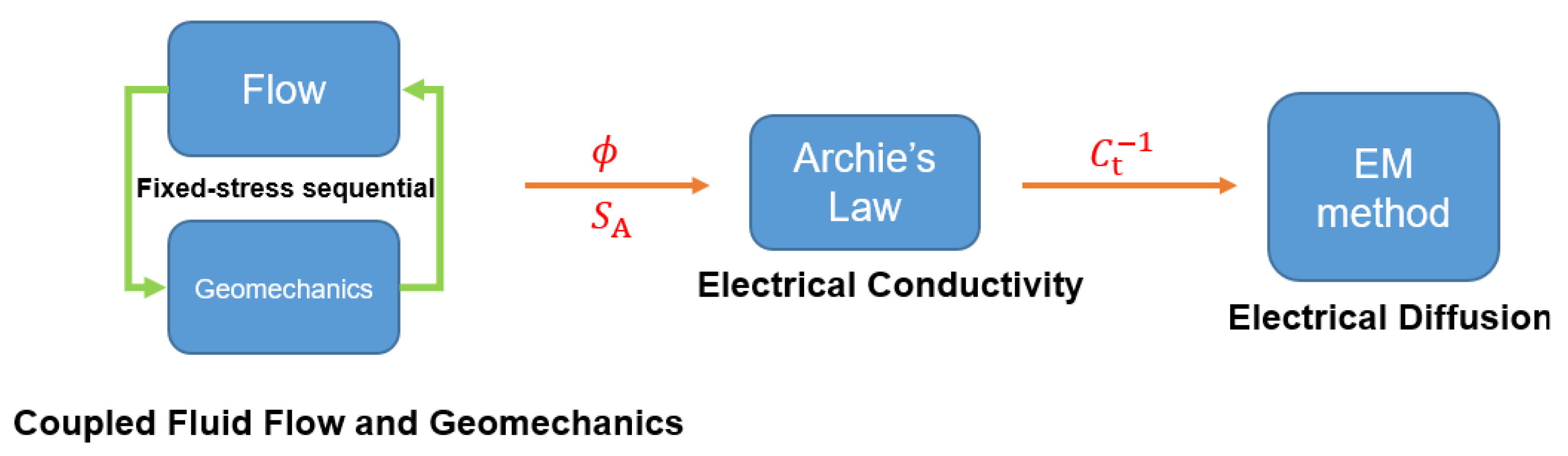
3. Numerical Methods

Numerical methods chosen for the integrated flow-geomechanics-EM geophysics simulation are briefly introduced. For the heavy nonlinearities that may occur not only in the coupled flow and geomechanics but also in the EM geophysics simulations, the Newton method is employed in each problem for convergence within a timestep.

3.1. Coupled Flow and Geomechanics

3.1.1. Spatial and Temporal Discretizations

In this study, we employ the finite volume method (FVM) and the finite element method (FEM) for non-isothermal multiphase multicomponent fluid/heat flow and geomechanics for their spatial discretizations, respectively. For spatial discretizations, this pair is known for yielding better numerical stability in space [23] compared to the same order of FEM for both flow and geomechanics. Furthermore, it is practical because the FEM is widely adopted in the geotechnical engineering community and the FVM is chosen for most reservoir simulators. We employ the backward Euler method for time discretization, which is also widely used for reservoir simulation [43].

3.1.2. Fixed-Stress Sequential Method

We use a sequential method called the fixed-stress method, which is unconditionally stable and convergent [17,24], to solve the non-isothermal flow problem. The fixed-stress sequential method implicitly solves the flow problem first by fixing the rate of total stress with the variation of the strain and displacement fields allowed. It then solves the geomechanics problem implicitly based on the intermediate solution from the previous non-isothermal flow problem until reaching the convergence.

The fixed-stress method is modified for the MP model as in the previous study [3,17] to solve coupled flow and geomechanics [28]. Equation (23) with the Lagrange porosity function and its correction is then linearized as

$$\begin{array}{ccc}\hfill {{\Phi }_l}^{n+1}-{{\Phi }_l}^n+\Delta {\Phi }_l& =& \underset{{\Phi }_l^n{c}_p}{\underbrace{\left\{\frac{{\alpha }_l^2}{K_l}+\frac{{\alpha }_l-{\Phi }_l^n}{K_s}\right\}}}\sum _{J=A,G}{\displaystyle \frac{S_J^{n+1}}{S_F^{n+1}}}\left(p_{l,J}^{n+1}-p_{l,J}^n\right)+3{\alpha }_T^l{\alpha }_l\left(T_l^{n+1}-T_l^n\right),\hfill \end{array}$$

(27)

$$\begin{array}{ccc}\hfill \Delta {\Phi }_l& =& {\displaystyle \frac{b_l}{{\eta }_l}}({\sigma }_v^{l,n}-{\sigma }_v^{l,n-1}),\hfill \end{array}$$

(28)

where $c_p$ is the pore compressibility for the uncoupled flow simulation, and the superscript n indicates the time level. Note the porosity correction term, $\Delta {\Phi }_l$, can correct the inconsistency (i.e., the porosity difference) between the uncoupled flow problem with the pore compressibility and the geomechanics with the strain.

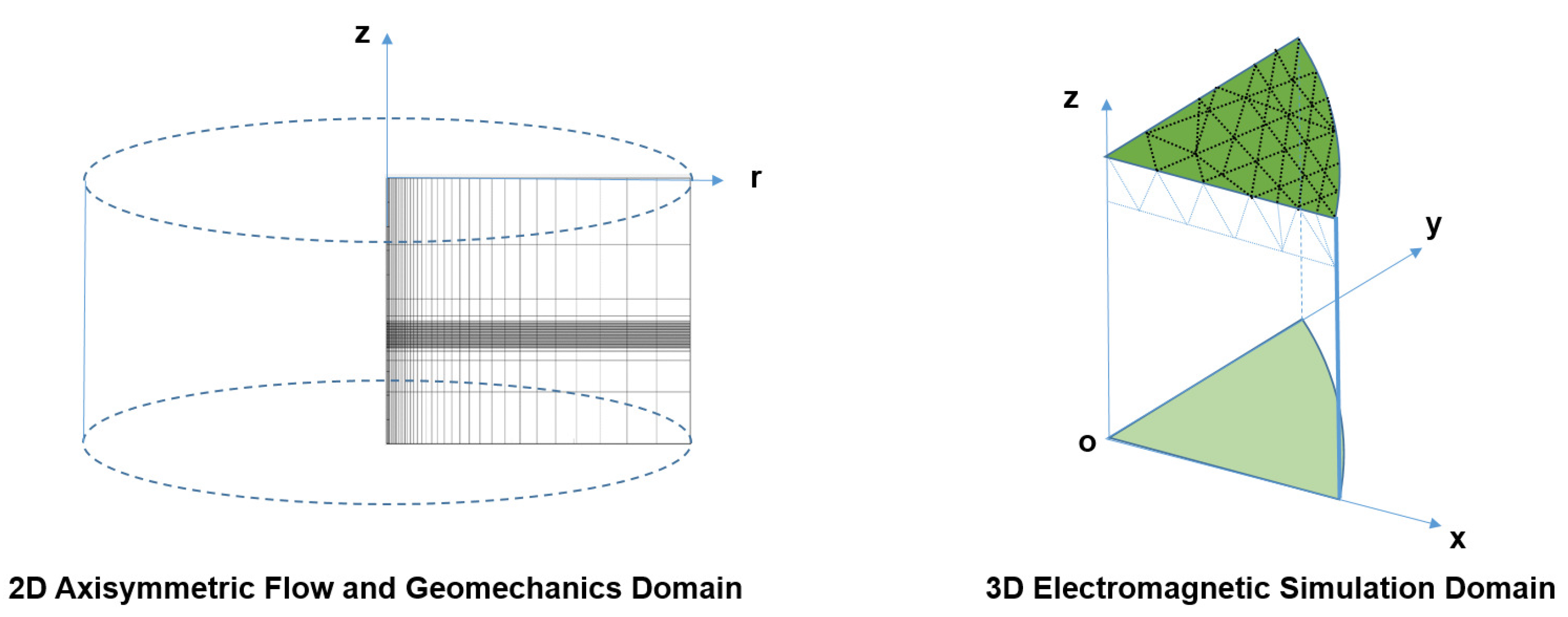
3.2. Electrical and EM Geophysical Modeling

We employ the finite element formulation [25] for solving the electric-field diffusion equation (see Equation (24)). For the time disretization, the backward Euler method is also employed. The resulting linearized system is then symmetric and positive definite, which can be efficiently solved using an adaptive time-stepping algorithm with a Cholesky factorization [44,45]. Once the potential, i.e., ${\varphi }_{em}\left(\mathit{r}\right)$, at each node is determined, the electric field, i.e., $\mathit{e}$, is calculated by dividing potential difference by their distance between two adjacent nodes. Note that any inversion of the electrical field is not considered in this study.

4. Numerical Experiments

In this section, numerical experiments are conducted using the integrated flow-geomechanics-EM geophysics simulation aiming at a specific heterogeneous layered gas hydrate deposit, located near the site UBGH2-6, the Ulleung Basin, East Sea, Korea. The schematic flow chart of the integrated simulation proposed in this study is depicted in Figure 1.

Regarding coupled flow and geomechanics for the field-wide simulation first, we use, respectively, the TOUGH+HYDRATE simulator [20] and the ROCMECH [22], which is an in-house simulator. For the two-way coupling between the fluid with heat and geomechanics, we employ the aforementioned fixed-stress sequential method—the unconditionally stable and convergent sequential method [24]—to overcome the stability issues that may occur for a sequential method depending on the coupling strength. To avoid further spurious numerical instability in space at the early time of simulation, the mixed formulation, i.e., the FEM for geomechanics and the FVM for fluid flow are employed for their space discretizations. The implicit–implicit Euler method is applied for time discretization. For the elastoplastic regime in the geomechanics, we employ the Mohr–Coulomb failure model for the elastoplasticity regime in the ROCMECH within the small deformation theory and the infinitesimal transformation. By coding the interface formulation using Equation (28), we can then capture the changes in reservoir pressure due to compaction of the reservoirs, such as the Mandel–Cryer effect [28,46]. Note that the heat and geomechanics are loosely coupled with the one-way coupling, for which from heat to geomechanics only is considered. The effects on the heat flow from geomechanics can be accounted for through the changes in the fluid flow. Note also that the MP model [3,17] is applied, which is straightforward due to the sequentially coupled system and particularly to the ROCMECH’s in-house property. Specifically for the MP model in this study, the MP4 model is used following the work in [3]. For the detailed descriptions of the MP model, we refer the readers to [3].

Figure 2 illustrates the numerical domains for the coupled flow-geomechanical and the EM geophysics simulations: the 2D axisymmetric and the 3D Cartesian domains, respectively. To compute the stress and deformation precisely, particularly near the wellbore, the exact 2D axisymmetric formulation for geomechanics is applied with the cylindrical coordinate system for momentum balance. For the EM simulation, this cylindrical coordinate system with the radius (r) from the z-axis is converted to the x and y based on the relation, i.e., $r^2=x^2+y^2$. Through the EM simulation in the 3D Cartesian domain, the diffusive EM field is then obtained using the diffusion model (Equation (24)) for the electric field. Note that we employ the 3D finite element method (FEM) [25,26,37] with unstructured tetrahedral grids to accurately handle irregular gas hydrate plume not conforming to rectangular Cartesian grids.

Numerical output from the coupled flow-geomechanical simulation while CH${}_4$ is extracted from the hydrates is the input for the rock physics model, for which Archie’s law is employed in this study (see Figure 1). Hydrological and petrophysical parameters, i.e., changes of aqueous phase saturation and porosity, are then transformed into the electrical conductivity model.

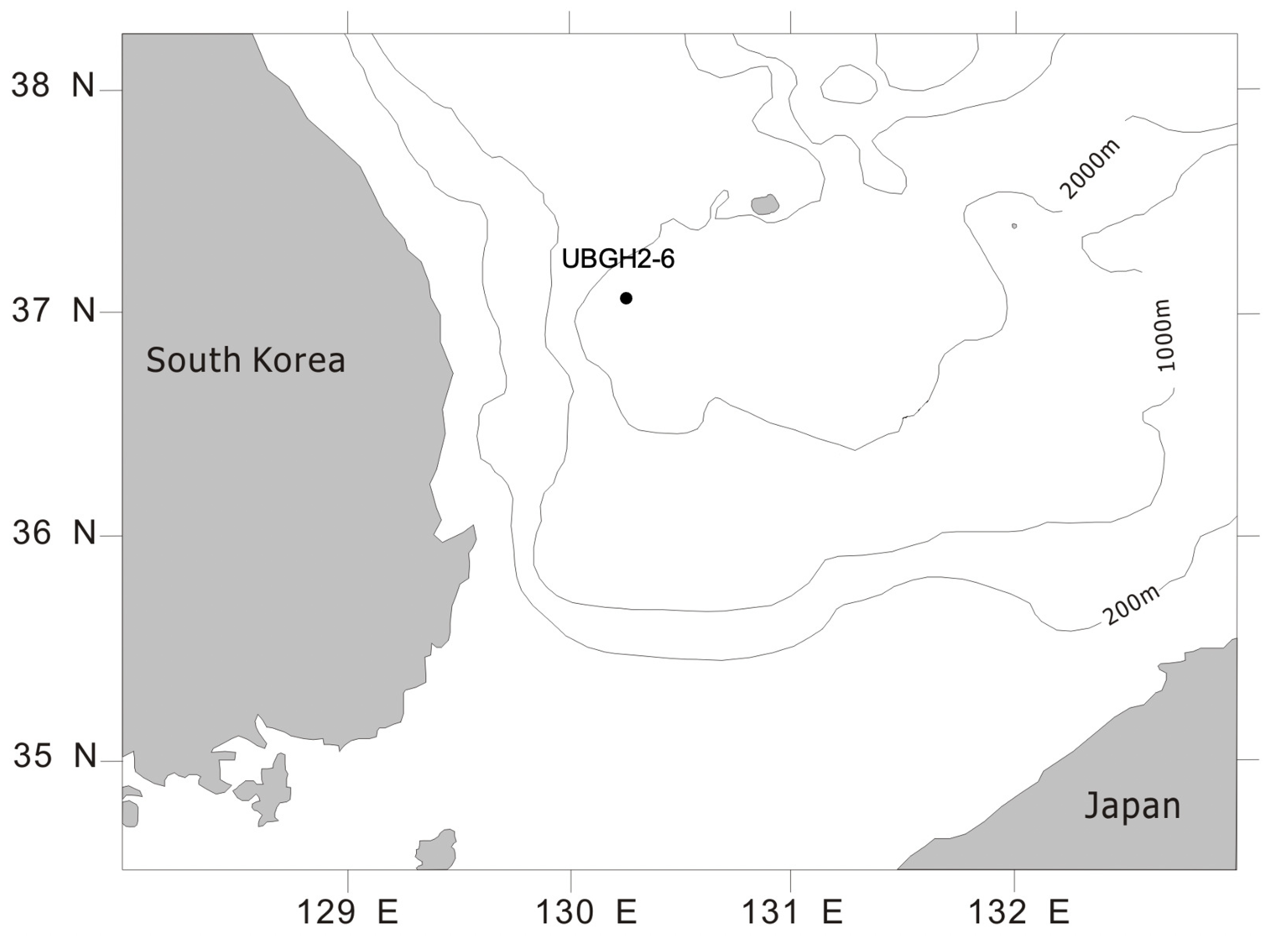
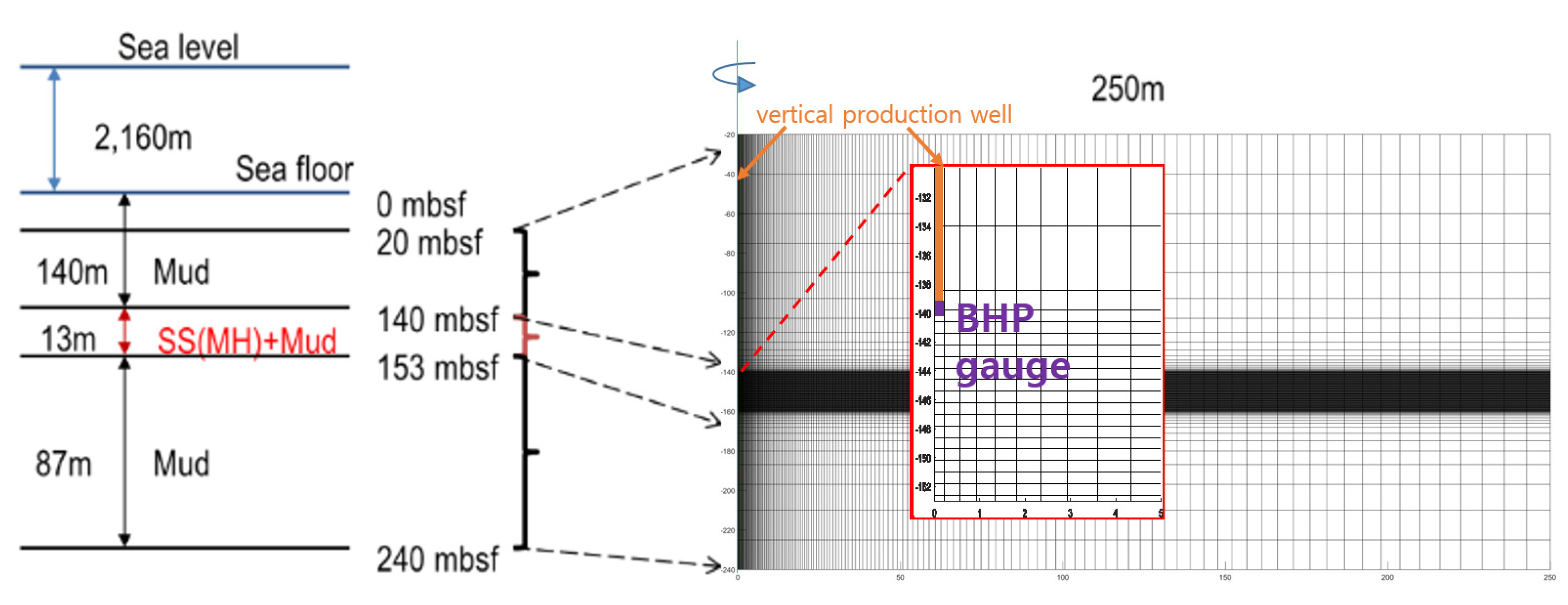
4.1. Gas Hydrate Deposit Located near the Site of the UBGH2-6 in the Ulleung Basin

For the applicability of electromagnetic (EM) geophysics methods in the field-wise simulation, a gas hydrate deposit located near the site UBGH2-6 in the Ulleung Basin is chosen following the previous study [3]. As shown in Figure 3 and Figure 4, the site UBGH2-6 is near the sea floor at approximately 140 mbsf under the East Sea, South Korea. Having a significant overburden in the deep sea with the water depth of about 2.1 km, the thickness of hydrate reservoir under study is relatively thin such that the producing interval is from 140 mbsf to 153 mbsf (13 m). Moreover, it is even heterogeneous, intercalated with alternating hydrate-bearing sand and mud layers. This model is from the UBGH2 expedition [47,48,49,50], and the parameters were estimated from the logging and core data obtained in the expedition.

We confine the heterogeneity of the hydrate reservoir to the vertical one with intercalated layers of two types of deposit: sand and mud. These two deposits are assumed to have different permeabilities and geomechanical moduli as geological porous media; values of which can change based on the hydrate saturation (S${}_H$) from zero to unity. Particularly, the geomechanical properties can be critically dependent on hydrate saturation [51,52,53,54]. Extending the previous study for the hydrate deposits in Mallik (Canada) and Mount Elbert, which were from the experimental results of Masui et al. [51,52] and involved a numerical simulation [55], we follow the power law relation between the drained bulk/shear moduli and hydrate saturation, written

$$\begin{array}{cc}\hfill & K_{dr}\left(S_S\right)=K_{dr}(S_S=0)+(K_{dr}(S_S=1)-K_{dr}(S_S=0))\times S_S^{n_k},S_S=S_I+S_H,\hfill \end{array}$$

(29)

$$\begin{array}{cc}\hfill & G_{dr}\left(S_S\right)=G_{dr}(S_S=0)+(G_{dr}(S_S=1)-G_{dr}(S_S=0))\times S_S^{n_g},\hfill \end{array}$$

(30)

where $n_k$ and $n_g$ are the exponents for material characterization, which are assumed to be unity in this study. $K_{dr}$ and $G_{dr}$ are the drained bulk modulus and the drained shear modulus, respectively, and $S_S$ is the saturation of solid phase consisting of the hydrate saturation ($S_H$) and the ice saturation ($S_I$).

Table 1. Material properties for flow and geomechanics in each type of layer for the simulation.

Layers	${\mathit{K}}_{\mathit{dr}}$ [MPa]		${\mathit{G}}_{\mathit{dr}}$ [MPa]		k [mD]	${\mathsf{\Phi }}_0$
	${\mathbf{S}}_{\mathit{H}}=0.0$	${\mathbf{S}}_{\mathit{H}}=1.0$	${\mathbf{S}}_{\mathit{H}}=0.0$	${\mathbf{S}}_{\mathit{H}}=1.0$	${\mathbf{S}}_{\mathit{H}}=0.0$	-
Overburden	15.55	285.0	5.185	99.75	0.02	0.76
Sand interlayer	27.0	933.33	16.0	560.0	500.0	0.45
Mud interlayer	20.0	285.0	6.667	99.75	0.14	0.67
Underburden	22.0	285.0	7.407	99.75	0.02	0.63

lists the main parameters of flow and geomechanics purely following the work in [3,15], which is not based on any direct measurement but based on a suitable estimate. The overall deposit that includes hydrate-bearing sand layers is simplified into four layers: overburden (Mud), (hydrate-bearing) sand interlayer (SS), mud interlayer (Mud), and underburden (Mud) (see Figure 4). Geomechanical properties, $K_{dr}$ and $G_{dr}$, follow Equations (29) and (), respectively. $\mathit{k}$ denotes the isotropic permeability value and ${\Phi }_0$ indicates the initial porosity. Within the sand layer, having its initial porosity of ${\Phi }_0=0.45$, we set the initial hydrate saturation buried identical to 0.65 (i.e., S${}_{H_0}$ = 0.65). For the rest of the pore space, it is fully saturated with the aqueous phase.

The computational domain for coupled flow and geomechanics simulation is two-dimentional (2D) axisymmetric. It has the size of 250 m × 220 m in the r- and z-directions, respectively, containing gridblocks of irregular size (160 × 140). Gas production via depressurization is then simulated from a vertical well with a BHP gauge assumed (colored in orange and purple, respectively, in Figure 4). In Figure 4, the intercalated layers of the reservoir correspond to the black-colored region, which is due to the extremely refined gridblocks for the reservoir with hydrate zones approaching the vertical well. Employing the MP4 model for the geomechanics following the work of [3], four vertical subelements construct one gridblock in the geomechanics, and it has 35 layers in the z-direction; thus, each layer has four sublayers (subelements) inside. Meanwhile, the original system of 140 gridblocks in the z-direction is still applied to the flow problem with the simulator TOUGH+HYDRATE. The initial pressures at the top (20 mbsf) and bottom (240 mbsf) are 23.1 MPa and 24.59 MPa, respectively, for which we follow the sign convention for stress such that tensile stress is positive. Considering the equilibrium state, the initial axial and radial stresses are then −23.1 MPa and −3.47 MPa, respectively, distributed vertically with the gradients of −25.0 kPa/m and −3.47 kPa/m. The initial temperatures are set also at the top and bottom as 6.366 ${}^{\circ }$C and 25.480 ${}^{\circ }$C, respectively. For the coupled flow and geomechanics numerical simulation, we apply a constant BHP of 9 MPa for the depressurization for 154 days of the production period. Regarding the boundary conditions, for the flow, we have no flow (Neumann type) boundary conditions over the entire boundary, whereas for the geomechanics, we have no displacement (Dirichlet type) condition, which is normal to each boundary except the top boundary where we have a traction (Neumann type) boundary condition.

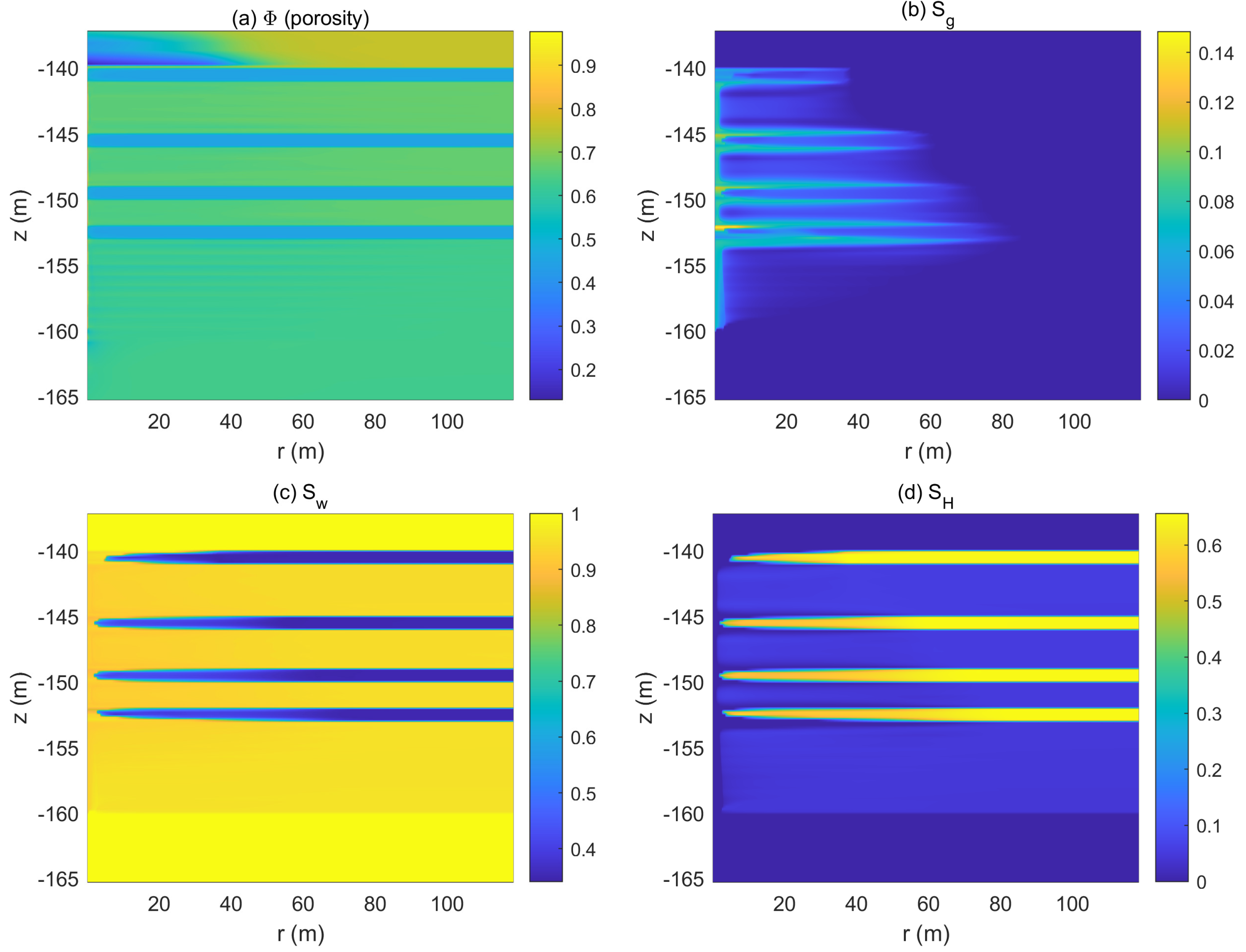
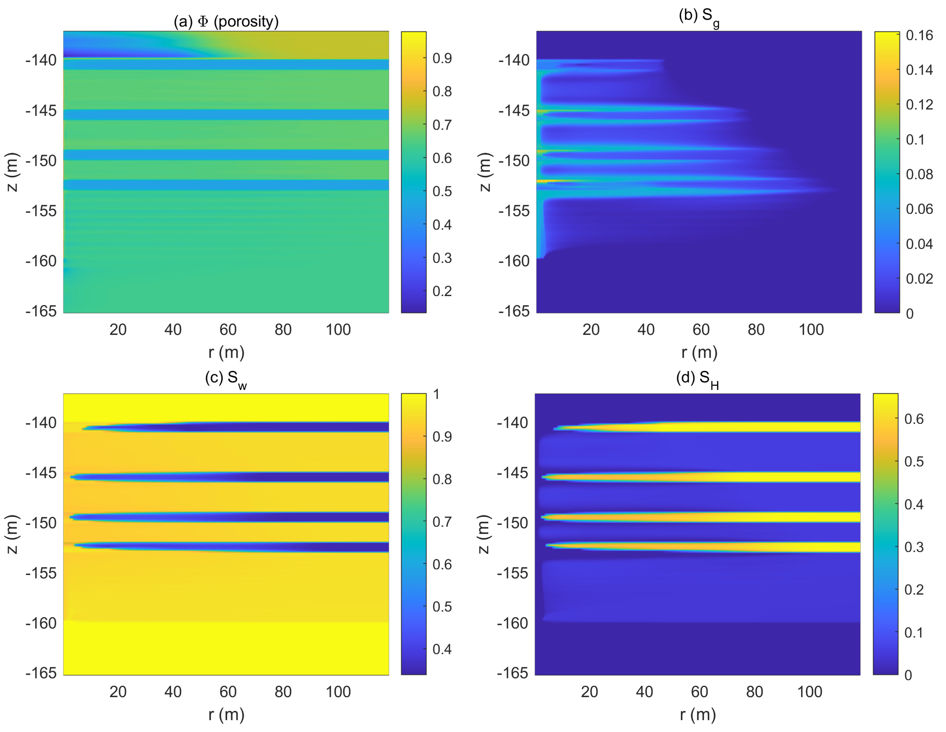
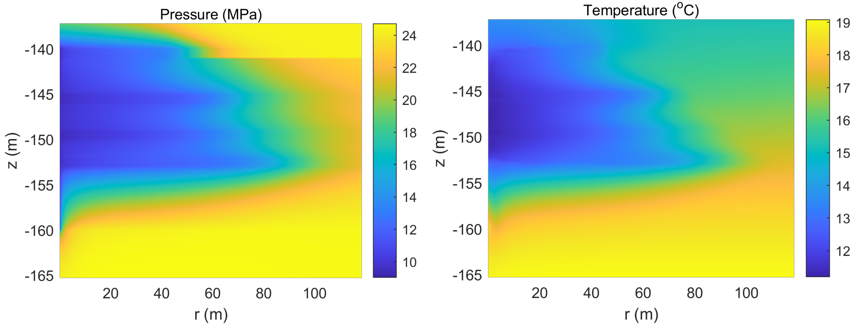
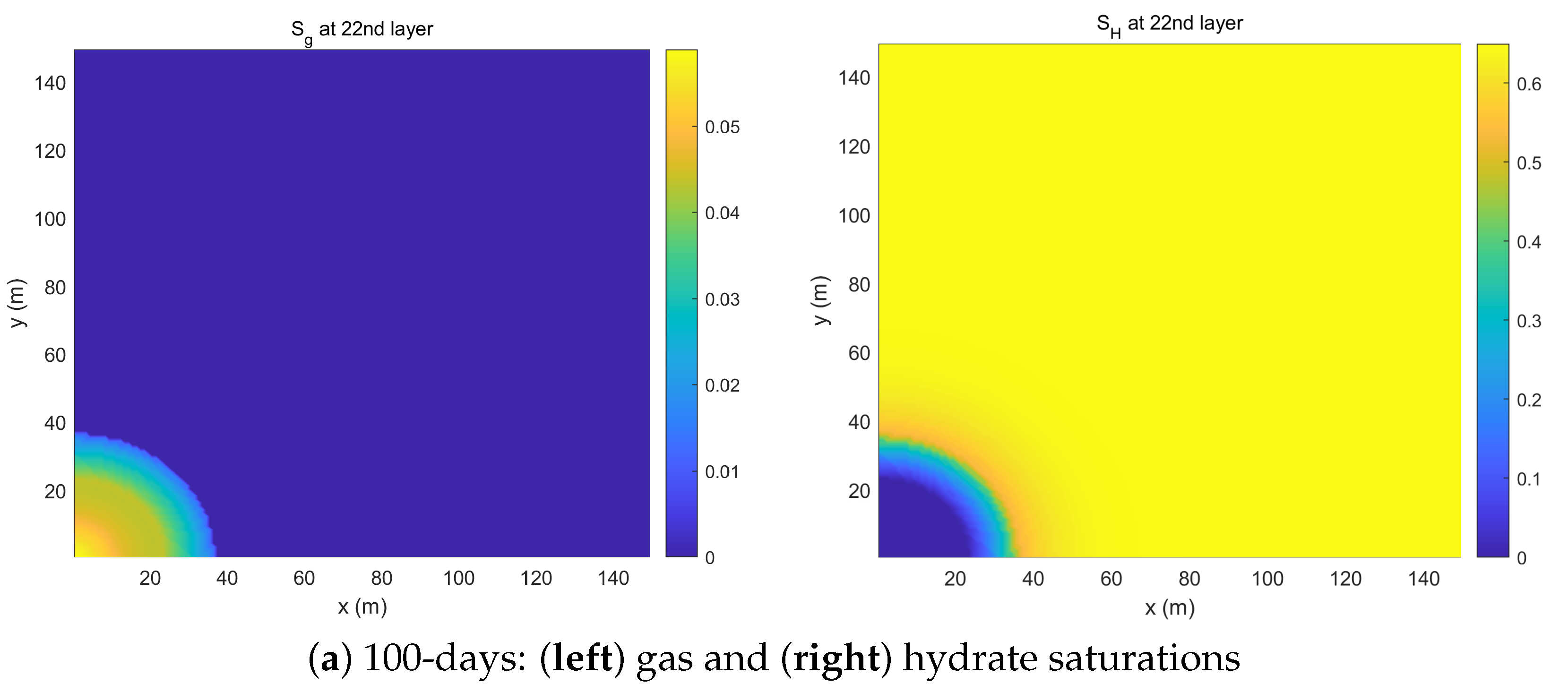
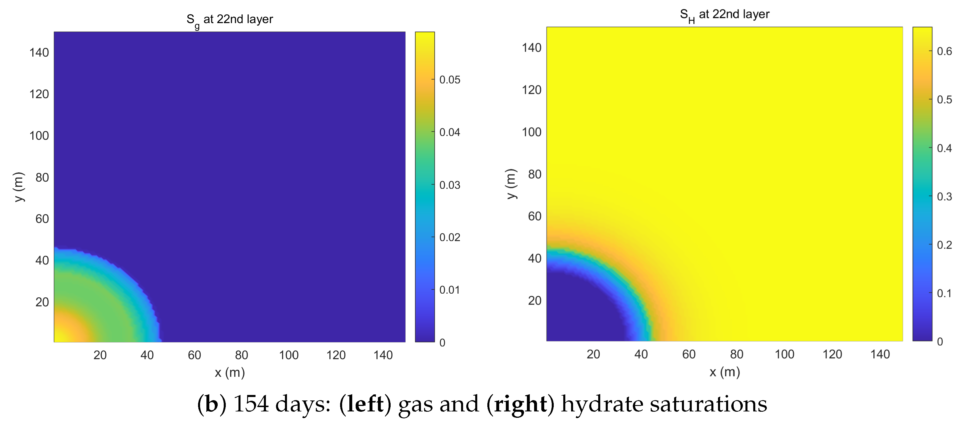
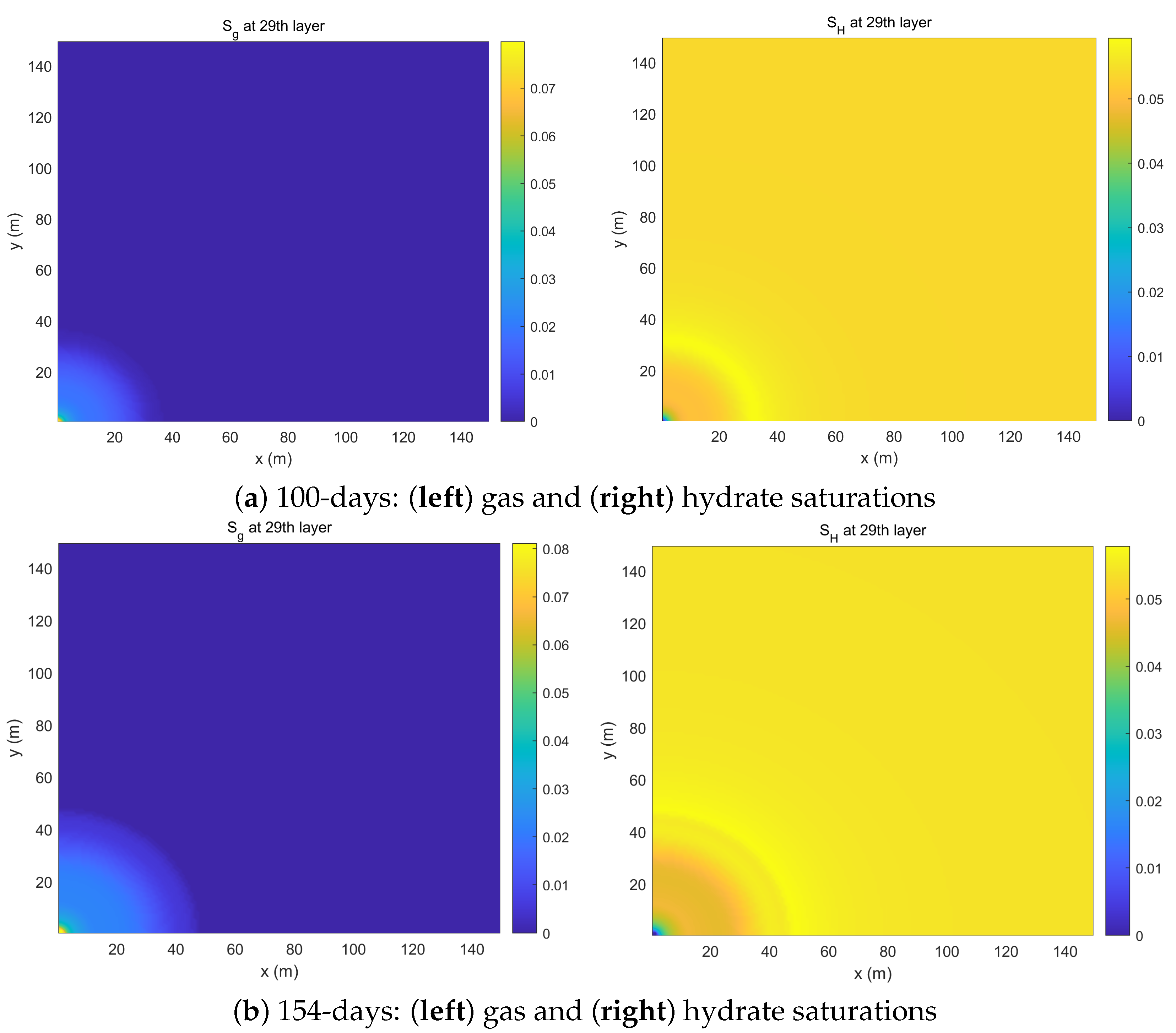
4.2. Evolution of Field Variables

Upon the information for the reservoir near the site UBGH2-6 and for the simulation of coupled fluid flow and geomechanics in Section 4.1, we first compare the evolution of porosity and saturation from their initial states after gas production for 100 days and 154 days. The initial state for saturation demonstrates that the fluid initially consists of the aqueous phase only, and the rest is filled with the solid phase of hydrates, i.e., S${}_{H_0}$= 0.65 and S${}_{A_0}$=0.35 inside the hydrate-bearing sand with the initial porosity of ${\Phi }_0=0.45$.

Figure 5, Figure 6 and Figure 7 illustrate the distributions of (a) porosity, (b) gas saturation, (c) water saturation, and (d) hydrate saturation at the initial time, after 100 days and after 154 days of production, respectively. Simply for comparison purposes, relatively short periods of time are chosen between Figure 6 and Figure 7. The employed MP4 model is confirmed to yield reliable results for the evolution of field variables with high computational efficiency and without any numerical instability. In porosity and saturation, distinctive results are obtained in the four hydrate-bearing sand layers where hydrate dissociations occur. As depressurization proceeds along with the gas production, compaction of both the hydrate and mud layers occurs severely, especially right next to the BHP gauge (see each (a) in Figure 5, Figure 6 and Figure 7), and gas saturation increases due to hydrate dissociation while hydrate saturation decreases. Small changes in saturation are found between (b) after 100 days and (c) after 154 days of production, which is due to a relative short time interval.

Figure 8 demonstrates the pressure and temperature distributions after 154 days of production. From temperature, the endothermic reaction is confirmed, along with the dissociation of gas hydrates as shown in each (c) in Figure 5, Figure 6 and Figure 7.

Figure 9 depicts gas (S${}_g$) and hydrate (S${}_H$) saturations in the converted 3D coordinate system (see Figure 2) within the 22nd layer (i.e., the first hydrate zone layer or SS in Figure 4) at the depth of 140.1 m, whereas Figure 10 is for the same at the 29th layer (i.e., the first mud zone layer or mud in Figure 4) at the depth of 141.5 m. In each figure, (a) after 100 days and (b) after 154 days are presented. In the mud, saturations of gas and hydrate are close to zero, whereas in the SS, we assume that hydrates are dissociated into the gas phase. We note that the overall saturation pattern between gas and hydrate are similar through the dissociations, which can deteriorate the sensitivity in calculation of the electrical resistivity field (see Section 4.3).

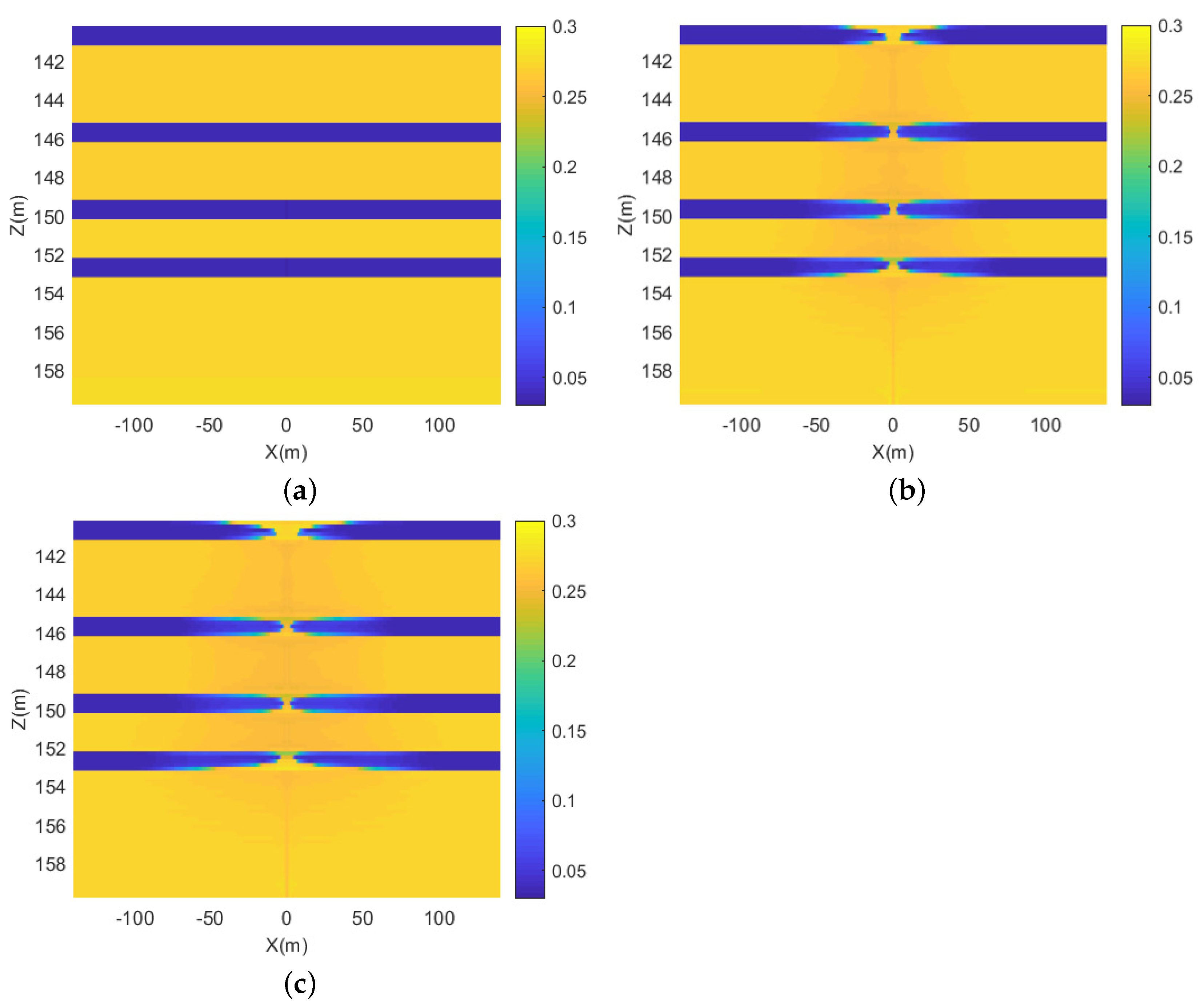
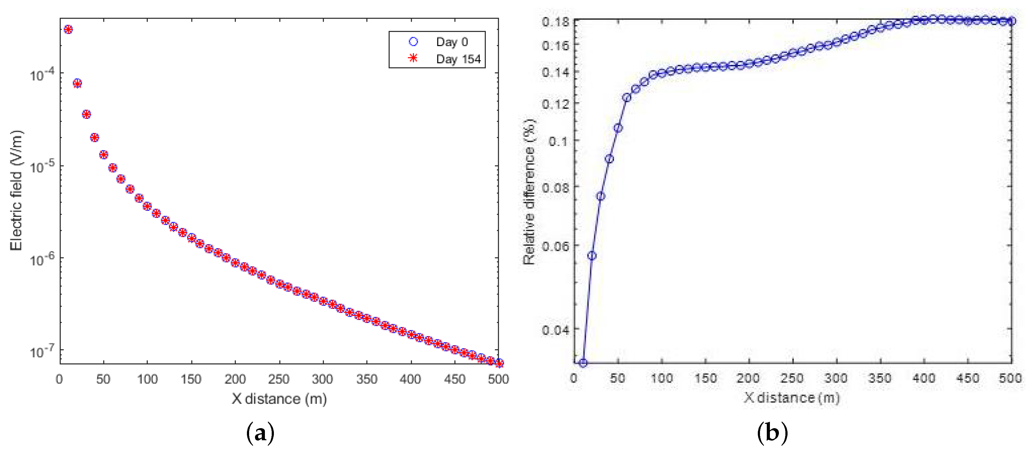
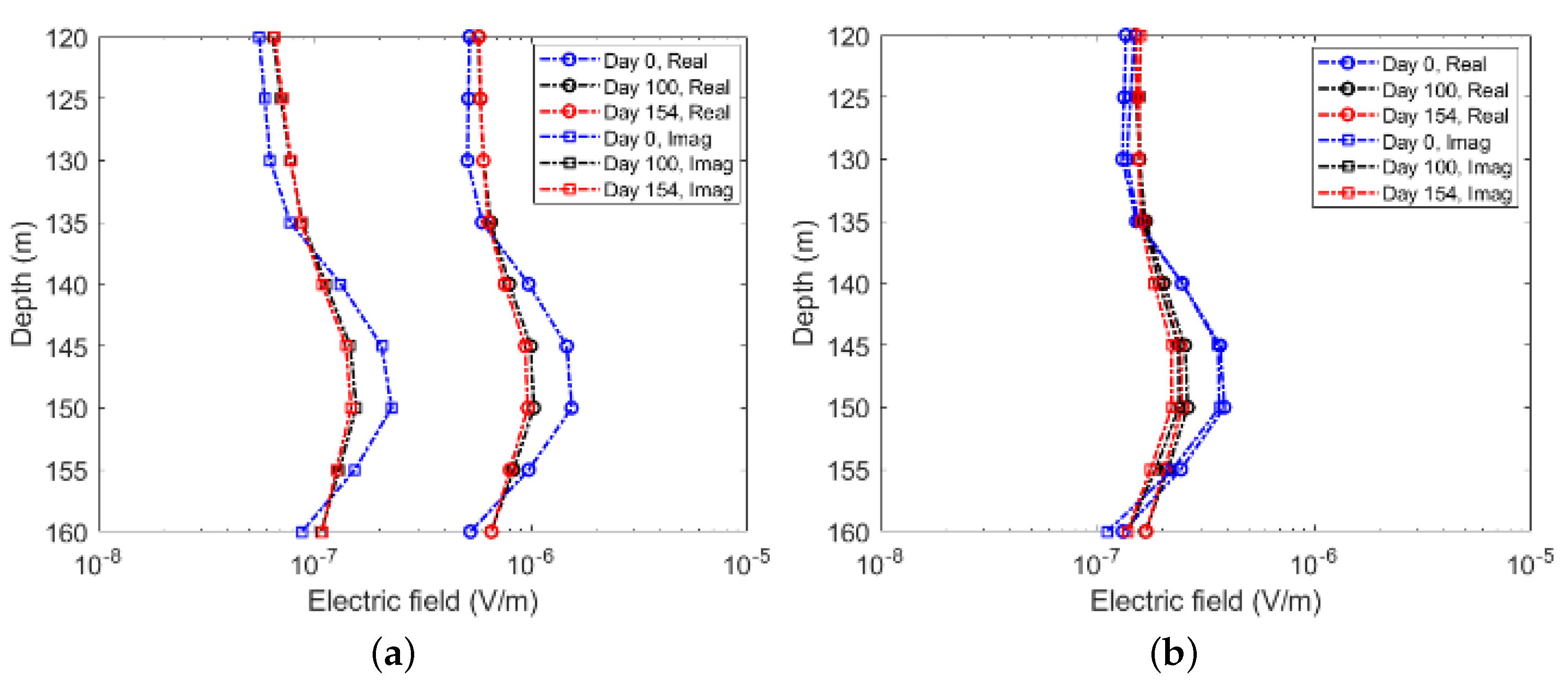
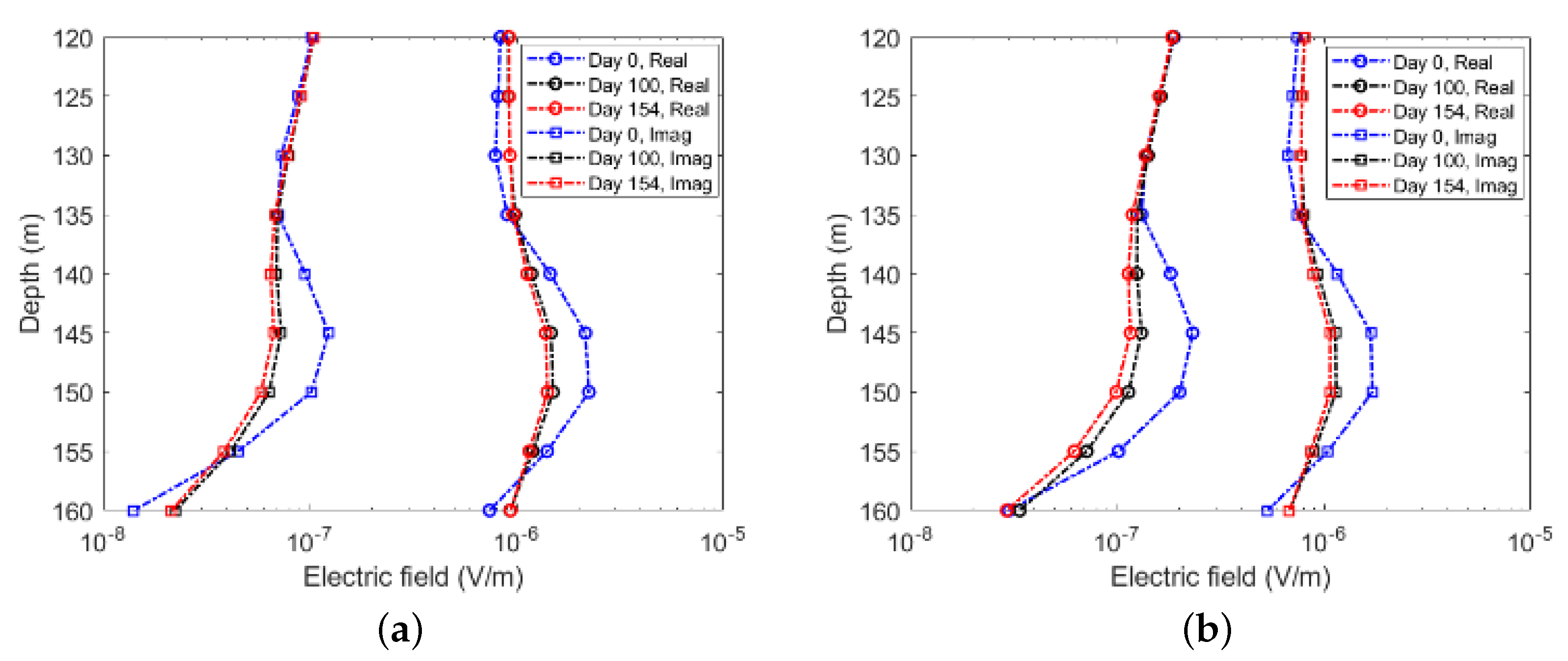
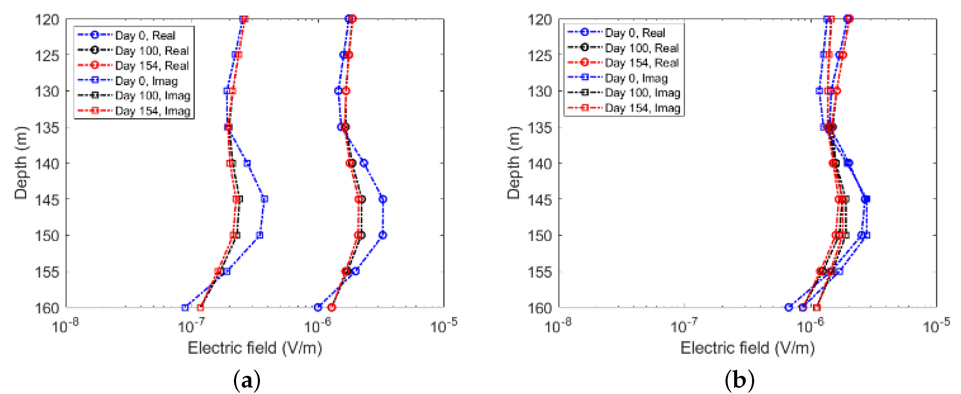
4.3. EM Monitoring Results and Detectability of Gas Flow

With the electrical conductivity field obtained via converting the hydrological and petrophysical parameters, the EM geophysics simulations are then conducted. As shown in Figure 2, numerical domains for the EM simulations are transformed into the 3D Cartesian where the 3D FEM with unstructured tetrahedral grids is employed.

The evolution of electromagnetic properties is mainly governed by the fluid-filled porosity, which is the function of porosity and hydrate saturation in hydrate deposits. The hydrate dissociation by depressurization can cause changes in fluid-filled porosity via the following mechanisms [56]: (a) phase changes from solid-phase hydrates to fluid phase gas and water will increase fluid-filled porosity, and thus electrical conductivity, (b) the sediment softening and volume contraction due to hydrate dissociation will decrease porosity and thus the electrical conductivity, and (c) the volume contraction under elevated vertical effective stress from depressurization of pore pressure. These complex mechanisms during hydrate dissociations often compensate the effect from each other, impairing the sensitivity of electromagnetic monitoring of hydrate dissociations.

Figure 11 depicts the electrical conductivity fields converted from the flow variables using Equation (25) at the corresponding times: (a) the initial state, (b) after 100 days, and (c) after 154 days. From these results, it can be inferred that the electromagnetic property changes due to the phase changes are the dominant mechanisms for this case among the mechanisms mentioned above, showing elevated conductivity distributions near the wellbore. Note that we can identify differences of the electrical conductivity results between the initial time, 100 days, and 154 days as the gas hydrate deposit dissociates around the well and subsequently the methane is extracted. However, in this very “early” production stage, the disk-shaped changes in the electrical conductivity are highly localized around the well. For example, on 100 days, the radius of the change in the top gas hydrate layer is about 8 m. In the second to fourth layers, the radii are just a few meters. It is even difficult to clearly distinguish the differences in the conductivity models between 100 and 154 days. Therefore, although the depth of the gas hydrate deposit is relatively shallow, it is challenging to detect the subtle change around the well.

In this study, we consider two EM monitoring configurations: surface-to-surface EM configuration utilizing a top-casing electric source and surface-to-borehole EM configuration as illustrated in Figure 12. As the name indicates, the primary difference lies in the location of the EM survey sensors; in our case, the surface-to-surface has it on the sea floor, i.e., 0 mbsf, whereas the surface-to-borehole has it on the bottom of the wellbore, i.e., 140 mbsf where the BHP gauge is located. Particularly, the configuration of EM monitoring is important for the intercalated system as the deposit at the UBGH2-6 site, because the low conductive layer can often cloud the effect from the changes beyond the layer. For the surface-to-surface configuration, the electric dipole source directly energizes a steel-cased well. The EM energy, i.e., the electric current, flows along the highly conductive metallic well and directly interacts with the gas hydrate structures around the well. The resulting electric fields are measured on or above the seafloor. The motivation behind this configuration is that the well plays the role of the vertical borehole electric source. The configuration mimics a surface-to-borehole EM configuration without requiring a well intervention. The surface-to-borehole configuration method has the horizontal electric dipole (HED) source, and EM sensors are placed in a well close to the gas hydrate deposits in contrast at the expense of well intervention and ensures the best possible sensitivity to the target. Albeit its current high expense, recent advances in cable-based EM sensing would make it economically feasible to measure EM fields inside/outside the well in the foreseeable future as fiber optic sensing technologies do in seismic data acquisition.

Figure 13 shows the results of electric fields at the initial time and after 154 days when the seafloor-to-seafloor configuration is employed: (a) absolute vales and (b) their relative difference. The two results from the corresponding times are nearly identical, and we cannot see sufficient sensitivity in the surface-to-surface configuration for detecting hydrate dissociation. A primary reason for this low sensitivity is that the injected currents mostly leak off from the well in shallow depth above the hydrate deposits due to high electrical conductivity in the seafloor environment. Moreover, the low detectability using the surface-to-surface configuration can also result from specific aspects of the study, such as small changes in saturation due to short production time and similar electrical resistivity values between gas and hydrate with a similar pattern of preferential horizontal dissociation, not vertical dissociation, from the intercalated reservoir near the UBGH2-6 site.

On the other hand, we observe sufficient sensitivity when we consider the seafloor-to-borehole configuration. In Figure 14, Figure 15 and Figure 16, each show electric field responses at different source positions when two different frequencies are used (10 Hz and 100 Hz at the left and right columns, respectively). The square marker in the legend stands for the imaginary (Imag) and the circle marker denotes the real (Real) for the complex numbers. Both frequencies can clearly capture dissociation of gas hydrates at the hydrate bearing layers (especially from 140 mbsf to 153 mbsf). Meanwhile, we observe less sensitivity between 100 days and 154 days because of very small changes in saturation during a short period of time (Figure 5, Figure 6 and Figure 7 and Figure 9), for which inverse modeling of these data can delineate changes in the gas hydrate deposit over time.

5. Conclusions

We study the feasibility of EM monitoring techniques for detecting dissociation of gas hydrates when gas is produced by depressurization. For the integrated flow-geomechanics-EM geophysics simulation, the evolution of saturation and porosity results obtained from coupled flow and geoemechanics simulation are converted into the electrical conductivity. Taking its inverse, the electrical resistivity and input parameter are made for the EM simulation using the electrical diffusion equation. Unlike the work in [13,27], the inversion of this calculated electric field is not considered in this study.

From numerical experiments with the field-wide simulation of a gas hydrate deposit in the Ulleung Basin, East Sea, Korea for natural gas production via depressurization, we identify that the EM survey sensitivity mainly depends on:

• Volume fraction of fluid phase and porosity change.
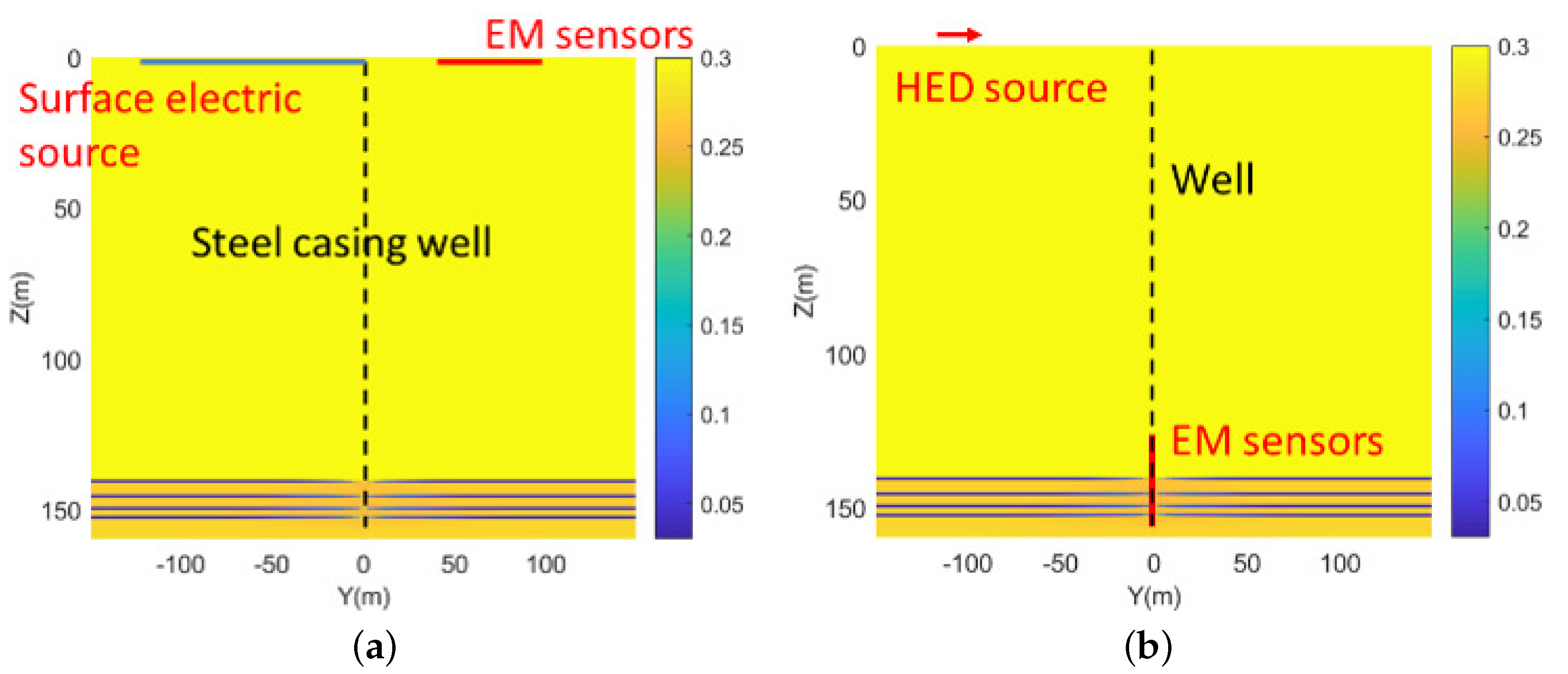
• EM survey configuration.
• Dissociation pattern of gas hydrates.

Although the conductivity model is uncertain, a more reliable conductivity equation is required considering severe porosity changes (i.e., large compaction) in the unconsolidated gas hydrate reservoir (e.g., near the site of UBGH2-6); the EM methods can further be utilized to estimate the bulk amount of gas extraction/production from the gas hydrate deposits and to evaluate any unfavorable potential leak of methane during production. Although statistical results are not presented in this contribution, distinct trends can be inferred, such as for the total average saturation rate of gas or the porosity change. It can even be indirectly calculated from Figure 9 and Figure 11. For example, the electrical conductivity of the hydrate deposit around the well after 154 days shows approximately 0.3, which is six times larger than the initial conductivity of 0.05. Similarly, the average pressure and temperature changes can be estimated over the entire simulation.

From the integrated flow-geomechanics-EM geophysics simulation proposed in this study, the different length scales of two simulations can be complementary to each other for a more precise characterization of gas flow. In essence, we can simulate responses of geomechanics and flow such as the surface deformation or pressure/failure around the well; the reservoir-scale changes over a larger volume of gas hydrate deposit can be monitored using the EM fields from the EM geophysics simulation. Therefore, this integrated flow-geomechanics-EM geophysics simulation can be a promising tool to monitor the evolution of gas hydrates, and its applicability can further reach other subsurface flow monitoring, such as the CO${}_2$ geological storage with an appropriate rock physics model.

References

1. Makogon, Y. Gas hydrates: Frozen energy. Recherche 1987, 18, 1192–1200. [Google Scholar]
2. Makogon, Y. Hydrates of Hydrocarbons; Penn Well Publishing Co.: Tulsa, OK, USA, 1997. [Google Scholar]
3. Yoon, H.; Yoon, S.; Lee, J.; Kim, J. Multiple porosity model of a heterogeneous layered gas hydrate deposit in Ulleung Basin, East Sea, Korea: A study on depressurization strategies, reservoir geomechanical response, and wellbore stability. J. Nat. Gas Sci. Eng. 2021, 96, 104321. [Google Scholar] [CrossRef]
4. Patti, G.; Grassi, S.; Morreale, G.; Corrao, M.; Imposa, S. Geophysical surveys integrated with rainfall data analysis for the study of soil piping phenomena occured in a densely urbanized area in eastern Sicily. Nat. Hazards 2021, 108, 2467–2492. [Google Scholar] [CrossRef]
5. Bretaudeau, F.; Dubois, F.; Kassa, S.G.; Coppo, N.; Wawrzyniak, P.; Darnet, M. Time-lapse resistivity imaging: CSEM-data 3-D double-difference inversion and application to the Reykjanes geothermal field. Geophys. J. Int. 2021, 226, 1764–1782. [Google Scholar] [CrossRef]
6. Yari, M.; Nabi-Bidhendi, M.; Ghanati, R.; Shomali, Z.H. Hidden layer imaging using joing inversion of P-wave trave-time and electrical resistivity data. Near Surf. Geophys. 2021, 19, 297–313. [Google Scholar] [CrossRef]
7. González, J.; Comte, J.C.; Legchenko, A.; Ofterdinger, U.; Healy, D. Quatification of groundwater storage heterogeneity in weathered/fractured basement rock aquifers using electrical resistivity tomography: Sensitivity and uncertainty associated with petrophysical modelling. J. Hydrol. 2021, 593, 125637. [Google Scholar] [CrossRef]
8. Glaser, D.; Burch, K.; Brinkley, D.; Reppert, P. Localization of deep voids through geophysical signatures of secondary dewatering features. Geophysics 2021, 86, WA139–WA152. [Google Scholar] [CrossRef]
9. Weitemeyer, K.; Constable, S.; Key, K.; Behrens, J. First results from a marine controlled-source electromagnetic survey to detect gas hydrates offshore Oregon. Geophys. Res. Lett. 2006, 33. [Google Scholar] [CrossRef] [Green Version]
10. Weitemeyer, K.; Constable, S.; Tréhu, A. A marine electromagnetic survey to detect gas hydrate at Hydrate Ridge, Oregon. Geophys. J. Int. 2011, 187, 45–62. [Google Scholar] [CrossRef] [Green Version]
11. Attias, E.; Weitemeyer, K.; Hölz, S.; Naif, S.; Minshull, T.; Best, A.; Haroon, A.; Jegen-Kulcsar, M.; Berndt, C. High-resolution resistivity imaging of marine gas hydrate structures by combined inversion of CSEM towed and ocean-bottom receiver data. Geophys. J. Int. 2018, 214, 1701–1714. [Google Scholar] [CrossRef]
12. Vermylen, J.; Zoback, M. Hydraulic Fracturing, Microseismic Magnitudes, and Stress Evolution in the Barnett Shale, Texas, USA. In Proceedings of the SPE Hydraulic Fracturing Technology Conference, The Woodlands, TX, USA, 24–26 January 2011. [Google Scholar]
13. Um, E.; Kim, J.; Wilt, M.; Commer, M.; Kim, S.S. Finite element analysis of top-casing electric source method for imaging hydraulically active fracture zones. Geophysics 2019, 84, E23–E35. [Google Scholar] [CrossRef] [Green Version]
14. Kim, J.; Um, E.; Moridis, G. Integrated simulation of vertical fracture propagation induced by water injection and its borehole electromagentic responses in shale gas systems. J. Pet. Sci. Eng. 2018, 165, 13–27. [Google Scholar] [CrossRef]
15. Moridis, G.J.; Kim, J.; Reagan, M.T.; Kim, S. Feasibility of gas production from a gas hydrate accumulation at the UBGH2-6 site of the Ulleung Basin in the Korean East Sea. J. Pet. Sci. Eng. 2013, 108, 180–210. [Google Scholar] [CrossRef]
16. Ryu, B.; Collett, T.; Riedel, M.; Kim, G.; Chun, J.; Bahk, J.; Lee, J.; Kim, J.; Yoo, D. Scientific results of the second gas hydrate drilling expedition in the Ulleung basin (UBGH2). Mar. Pet. Geol. 2013, 47, 1–20. [Google Scholar] [CrossRef]
17. Kim, J.; Sonnenthal, E.; Rutqvist, J. Formulation and sequential numerical algorithms of coupled fluid/heat flow and geomechanics for multiple porosity materials. Int. J. Numer. Methods Eng. 2012, 92, 425–456. [Google Scholar] [CrossRef] [Green Version]
18. Kurihara, M.; Ouchi, H.; Masuda, Y.; Narita, H.; Okada, Y. Assessment of Gas Productivity of Natural Methane Hydrates Using MH21 Reservoir Simulator. In Proceedings of the AAPG Hedberg Research Conference, Gas Hydrates: Energy Resource Potential and Associated Geologic Hazards, Vancouver, BC, Canada, 12–16 September 2004. [Google Scholar]
19. Kurihara, M.; Ouchi, H.; Masuda, Y.; Narita, H.; Okada, Y. Impact of Kinetics on the Injectivity of Liquid CO2 into Arctic Hydrates. In Proceedings of the OTC Arctic Offshore Technology Conference, Houston, TX, USA, 2–5 May 2011. [Google Scholar]
20. Moridis, G.J.; Kowalsky, M.B.; Pruess, K. TOUGH+HYDRATE v1.0 User’s Manual: A Code for the Simulation of System Behavior in Hydrate-Bearing Geologic Media; Report Number LBNL-00149E; Lawrence Berkeley National Lab.: Berkeley, CA, USA, 2008. [Google Scholar]
21. Kim, J.; Lee, J.; Ahn, T.; Yoon, H.; Lee, J.; Yoon, S.; Moridis, G. Validation of strongly coupled geomechanics and gas hydrate reservoir simulation with multiscale laboratory tests. Int. J. Rock Mech. Min. Sci. 2022, 149, 104958. [Google Scholar] [CrossRef]
22. Kim, J.; Moridis, G.J. Development of the T+M coupled flow-geomechanical simulator to describe fracture propagation and coupled flow-thermal-geomechanical processes in tight/shale gas systems. Comput. Geosci. 2013, 60, 184–198. [Google Scholar] [CrossRef]
23. Yoon, H.; Kim, J. Spatial stability for the monolithic and sequential methods with various space discretizations in poroelasticity. Int. J. Numer. Methods Eng. 2018, 114, 684–718. [Google Scholar] [CrossRef]
24. Kim, J.; Tchelepi, H.A.; Juanes, R. Stability and convergence of sequential methods for coupled flow and geomechanics: Fixed-stress and fixed-strain splits. Comput. Methods Appl. Mech. Eng. 2011, 200, 1591–1606. [Google Scholar] [CrossRef]
25. Um, E.; Commer, M.; Newman, G.; Hoversten, M. Finite element modeling of transient electromagnetic fields near steel-cased wells. Geophys. J. Int. 2015, 202, 901–913. [Google Scholar] [CrossRef] [Green Version]
26. Hughes, T.J.R. The Finite Element Method: Linear Static and Dynamic Finite Element Analysis; Prentice-Hall: Englewood Cliffs, NJ, USA, 1987. [Google Scholar]
27. Um, E.; Kim, J.; Wilt, M. 3D borehole-to-surface and surface electromagnetic modeling and inversion in the presence of steel infrastructure. Geophysics 2020, 85, E139–E152. [Google Scholar] [CrossRef]
28. Kim, J.; Moridis, G.J.; Yang, D.; Rutqvist, J. Numerical Studies on Two-way Coupled Fluid Flow and Geomechanics in Hydrate Deposits. SPE J. 2012, 17, 485–501. [Google Scholar] [CrossRef] [Green Version]
29. Kim, J.; Lee, J. Wellbore stability and possible geomechanical failure in the vicinity of the well during pressurization at the gas hydrate deposit in the Ulleung Basin. In Proceedings of the 53rd US Rock Mechanics/Geomechanics Symposium, New York, NY, USA, 26 June 2019. [Google Scholar]
30. Yoon, S.; Um, E.; Kim, J. Development of an integrated simulator for coupled flow, geomechanics and geophysics based on sequential approaches. J. Korean Soc. Miner. Energy Resour. Eng. 2020, 57, 309–317. [Google Scholar] [CrossRef]
31. Fawad, M.; Mondol, N. Monitoring geological storage of CO2: A new approach. Sci. Rep. 2021, 11, 5942. [Google Scholar] [CrossRef]
32. Coussy, O. Mechanics of Porous Continua; John Wiley and Sons: Chichester, UK, 1995. [Google Scholar]
33. Kim, J.; Tchelepi, H.A.; Juanes, R. Rigorous coupling of geomechanics and multiphase flow with strong capillarity. SPE J. 2013, 18, 1591–1606. [Google Scholar] [CrossRef]
34. Coussy, O. Poromechanics; John Wiley and Sons: Chichester, UK, 2004. [Google Scholar]
35. Commer, M.; Newman, G. New advances in three-dimensional controlled-source electromagnetic inversion. Geophys. J. Int. 2008, 172, 513–535. [Google Scholar] [CrossRef]
36. Um, E.; Kim, S.; Fu, H. A tetrahedral mesh generation approach for 3D marine controlled-source electromagnetic modeling. Comput. Geosci. 2017, 100, 1–9. [Google Scholar] [CrossRef]
37. Jin, J. The Finite Element Method in Electromagnetics, 2nd ed.; John Wiley and Sons: Hoboken, NJ, USA, 2002. [Google Scholar]
38. Si, H. TetGen, a Delaunay-Based Quality Tetrahedral Mesh Generator. ACM Trans. Math. Softw. 2015, 41, 11. [Google Scholar] [CrossRef]
39. Amestoy, P.; Duff, I.; L’Excellent, J.Y.; Koster, J. A fully asynchronous multifrontal solver using distributed dynamic scheduling. SIAM J. Matrix Anal. Appl. 2017, 23, 15–41. [Google Scholar] [CrossRef] [Green Version]
40. Archie, G. The electrical resistivity log as an aid in determining some reservoir characteristics. Trans. Am. Inst. Min. 1942, 146, 54–62. [Google Scholar] [CrossRef]
41. Yi, B.; Lee, G.; Kang, N.; Yoo, D.; Lee, J. Deterministic estimation of gas-hydrate resource volume in a small area of the Ulleung Basin, East Sea (Japan Sea) from rock physics modeling and prestack inversion. Mar. Pet. Geol. 2018, 92, 597–608. [Google Scholar] [CrossRef]
42. Mavko, G.; Mukerji, T.; Dvorkin, J. The Rock Physics Handbook; Cambridge University Press: New York, NY, USA, 2020. [Google Scholar]
43. Aziz, K.; Settari, A. Petroleum Reservoir Simulation; Elsevier: London, UK, 1979. [Google Scholar]
44. Golub, G.; Loan, C.V. Matrix Computations, 3rd ed.; Johns Hopkins University Press: Baltimore, MD, USA, 1996. [Google Scholar]
45. Saad, Y. Iterative Methods for Sparse Linear Systems, 2nd ed.; SIAM: Philadelphia, PA, USA, 2003. [Google Scholar]
46. Yoon, H.; Kim, J. Spectral deferred correction methods for high-order accuracy in poroelastic problems. Int. J. Numer. Anal. Methods Geomech. 2021, 45, 2709–2731. [Google Scholar] [CrossRef]
47. Bahk, J.J.; Kim, G.Y.; Chun, J.H.; Kim, J.H.; Lee, J.; Ryu, B.J.; Lee, J.H.; Son, B.K. Characterization of gas hydrate reservoirs by integration of core and log data in the Ulleung Basin, East Sea. Mar. Pet. Geol. 2013, 47, 30–42. [Google Scholar] [CrossRef]
48. Lee, J.S.; Lee, J.; Kim, Y.; Lee, C. Stress-dependent and strength properties of gas hydrate-bearing marine sediments from the Ulleung Basin, East Sea, Korea. Mar. Pet. Geol. 2013, 47, 66–76. [Google Scholar] [CrossRef]
49. Kim, H.S.; Cho, G.C.; Lee, J.; Kim, S.J. Geotechnical and geophysical properties of deep marine fine-grained sediments recovered during the second Ulleung Basin Gas Hydrate expedition, East Sea, Korea. Mar. Pet. Geol. 2013, 47, 56–65. [Google Scholar] [CrossRef]
50. Lee, J.; Kim, G.Y.; Kang, N.; Yi, B.Y.; Jung, J.; Im, J.H.; Son, B.K.; Bahk, J.J.; Chun, J.H.; Ryu, B.J.; et al. Physical properties of sediments from the Ulleung Basin, East Sea: Results from Second Ulleung Basin Gas Hydrate Drilling Expedition, East Sea (Korea). Mar. Pet. Geol. 2013, 47, 43–55. [Google Scholar] [CrossRef]
51. Masui, A.; Haneda, H.; Ogata, Y.; Aoki, K. The effect of saturation degree of methane hydrate on the shear strength of synthetic methane hydrate sediments. In Proceedings of the International Conference on Gas Hydrates (ICGH2005), Trondheim, Norway, 13–16 June 2005. [Google Scholar]
52. Masui, A.; Miyazaki, K.; Haneda, H.; Ogata, Y.; Aoki, K. Mechanical characteristics of natural and artificial gas hydrate bearing sediments. In Proceedings of the International Conference on Gas Hydrates (ICGH2008), Vancouver, BC, Canada, 6–10 July 2008. [Google Scholar]
53. Miyazaki, K.; Aoki, K.; Sakamoto, Y.; Yamaguchi, T.; Okubo, S. Study on Mechanical Behavior for Methane Hydrate Sediment Based on Constant Strain-Rate Test and Unloading-Reloading Test Under Triaxial Compression. Int. J. Offshore Polar Eng. 2010, 20, 256–264. [Google Scholar]
54. Miyazaki, K.; Masui, A.; Sakamoto, Y.; Tenma, N.; Yamaguchi, T. Effect of Confining Pressure on Triaxial Compressive Properties of Artificial Methane Hydrate Bearing Sediments. In Proceedings of the Offshore Technology Conference 2010, Houston, TX, USA, 3–6 May 2010. [Google Scholar]
55. Rutqvist, J.; Moridis, G.; Grover, T.; Collett, T. Geomechanical Response of Permafrost-associated Hydrate Deposits to Depressurization-induced Gas Production. J. Pet. Sci. Eng. 2009, 67, 1–12. [Google Scholar] [CrossRef] [Green Version]
56. Lee, J.; Santamarina, J.; Ruppel, C. Volume change associated with formation and dissociation of hydrate in sediment. Geochem. Geophys. Geosyst. 2010, 11, Q03007. [Google Scholar] [CrossRef]
Figure 1. Flow chart for the integrated coupled flow-geomechanics-EM geophysics simulation.
Energies 15 03823 g001
Figure 2. Numerical domains for the integrated coupled flow-geomechanics-EM simulation: (left) 2D axisymmetric domain with quadrilateral meshes for coupled flow and geomechanics and (right) 3D Cartesian domain with tetrahedral meshes converted for the EM simulation.
Energies 15 03823 g002
Figure 3. The UBGH2-6 site for gas hydrate reservoirs in the Ulleung Basin, East Sea, Korea [3].
Energies 15 03823 g003
Figure 4. (left) A schematic geological layer information of the hydrate deposit (the reservoir region with intercalated layers colored in red) in between the overburden and underburden muds, and (right) the numerical domain used for simulation as in [3].
Energies 15 03823 g004
Figure 5. Porosity and saturations of gas, water, and hydrate on day 0 (the initial state).
Energies 15 03823 g005
Figure 6. Porosity and saturations of gas, water, and hydrate after 100 days.
Energies 15 03823 g006
Figure 7. Porosity and saturations of gas, water, and hydrate after 154 days.
Energies 15 03823 g007
Figure 8. Pressure and temperature distributions after 154-days of production.
Energies 15 03823 g008
Figure 9. Gas and hydrate saturations in the converted 3D Cartesian domain at the 22nd layer within the SS: (a) after 100 days and (b) after 154 days. The origin is where the wellbore is located.
Energies 15 03823 g009aEnergies 15 03823 g009b
Figure 10. Gas and hydrate saturations in the converted 3D Cartesian domain at the 29th layer within the mud: (a) after 100 days and (b) after 154 days. The origin is where the wellbore is located.
Energies 15 03823 g010
Figure 11. Electrical conductivity models (unit: S/m): (a) after day 0 (the initial state), (b) after 100 days, and (c) after 154 days.
Energies 15 03823 g011
Figure 12. EM survey configuration: (a) the surface-to-surface monitoring, (b) the surface-to-borehole monitoring. Each legend bar represents the electrical conductivity (unit: S/m).
Energies 15 03823 g012
Figure 13. Comparison of electric fields between the initial time and after 154 days using the surface-to-surface configuration: (a) absolute values and (b) their relative difference.
Energies 15 03823 g013
Figure 14. Electric fields from the HED source using the surface-to-borehole method at (x,z) = (−300 m, −5 m) with two different Hz. (a) 10 Hz. (b) 100 Hz.
Energies 15 03823 g014
Figure 15. Electric fields from the HED source using the surface-to-borehole method at (x,z) = (−200 m, −5 m) with two different Hz. (a) 10 Hz. (b) 100 Hz.
Energies 15 03823 g015
Figure 16. Electric fields from the HED source using the surface-to-borehole method at (x,z) = (−100 m, −5 m) with two different Hz. (a) 10 Hz. (b) 100 Hz.
Energies 15 03823 g016