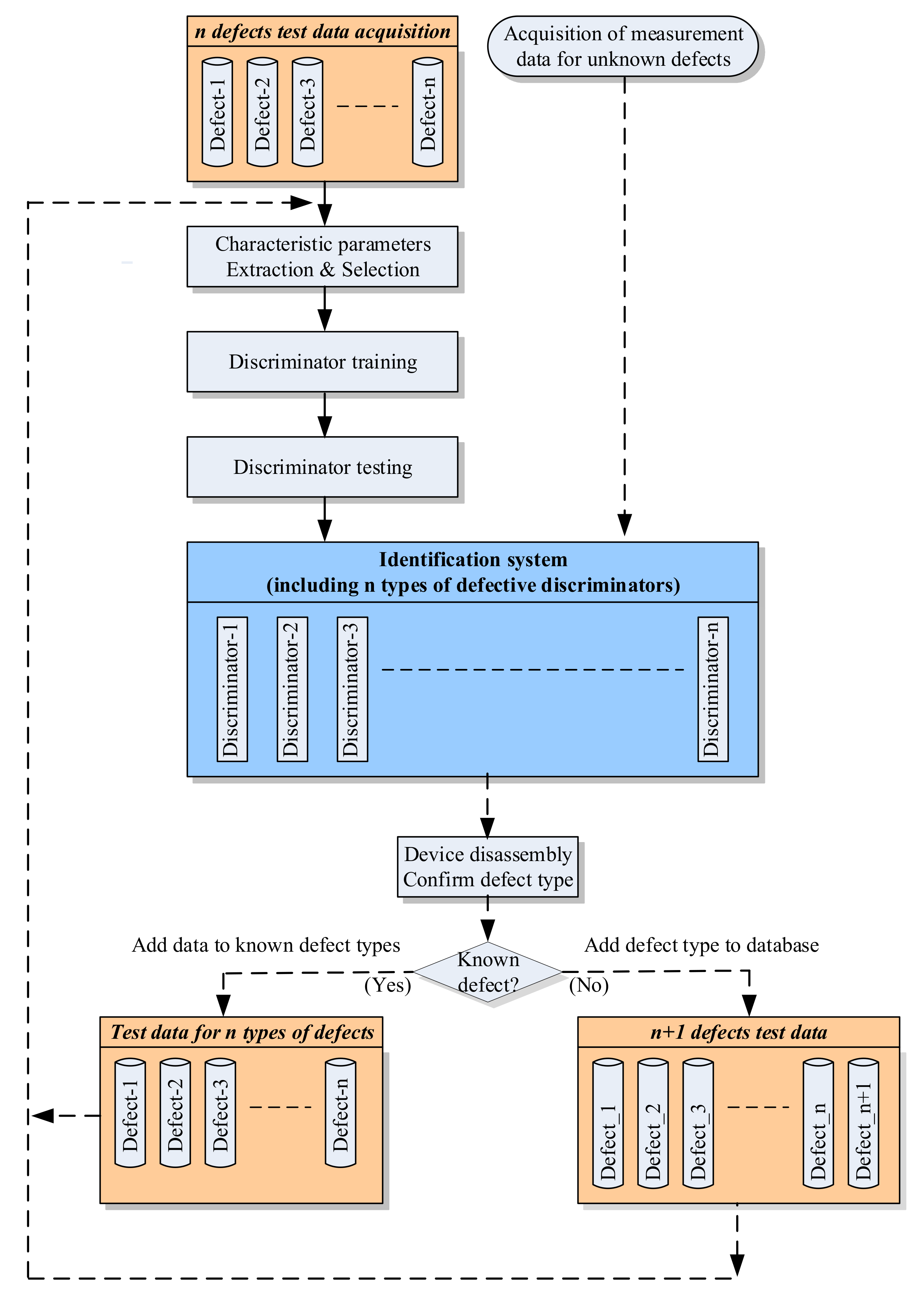
Figure 1.
Schematic diagram of the construction of a defect measurement database.
Figure 1.
Schematic diagram of the construction of a defect measurement database.
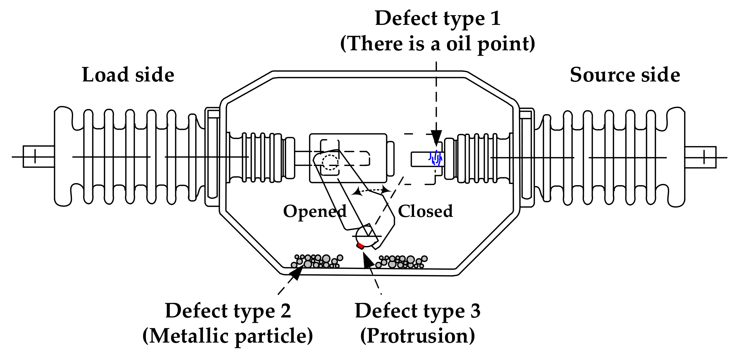
Figure 2.
Diagram of the internal defects of the switch.
Figure 2.
Diagram of the internal defects of the switch.
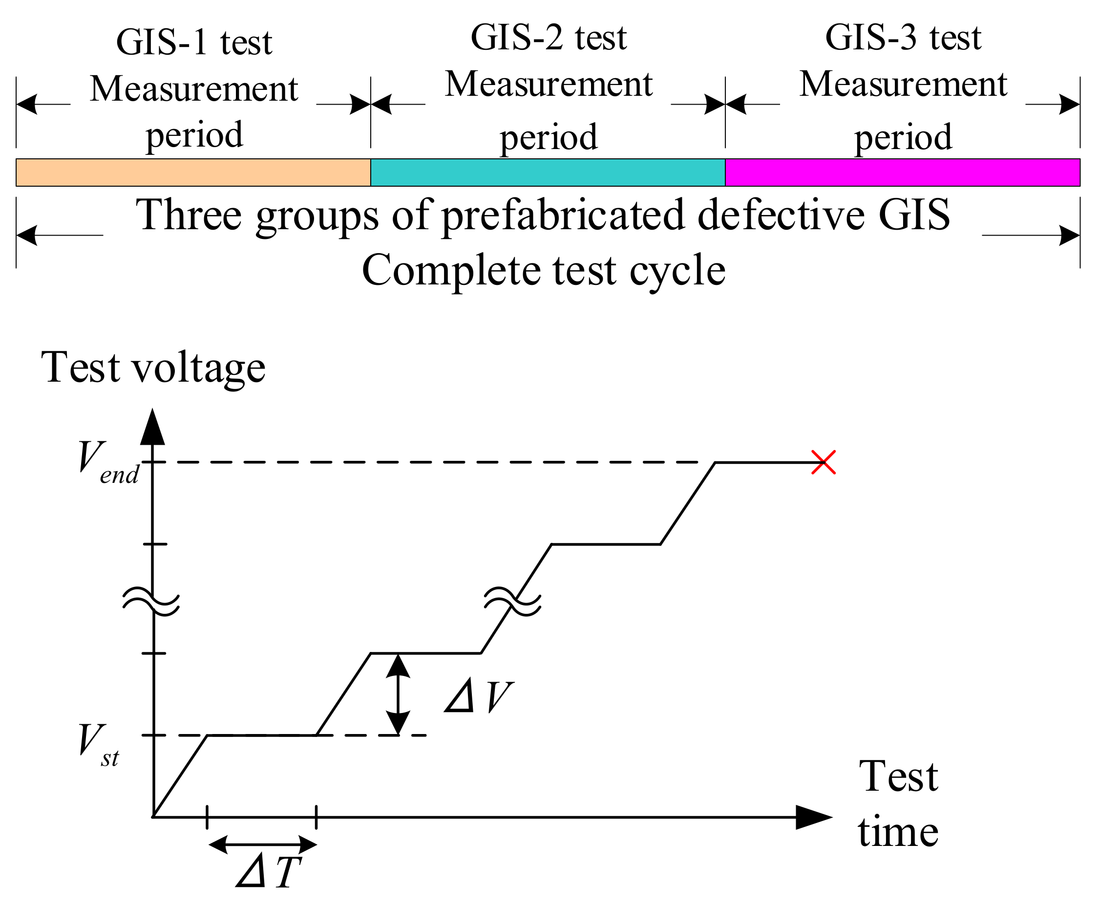
Figure 3.
Experimental planning concept.
Figure 3.
Experimental planning concept.
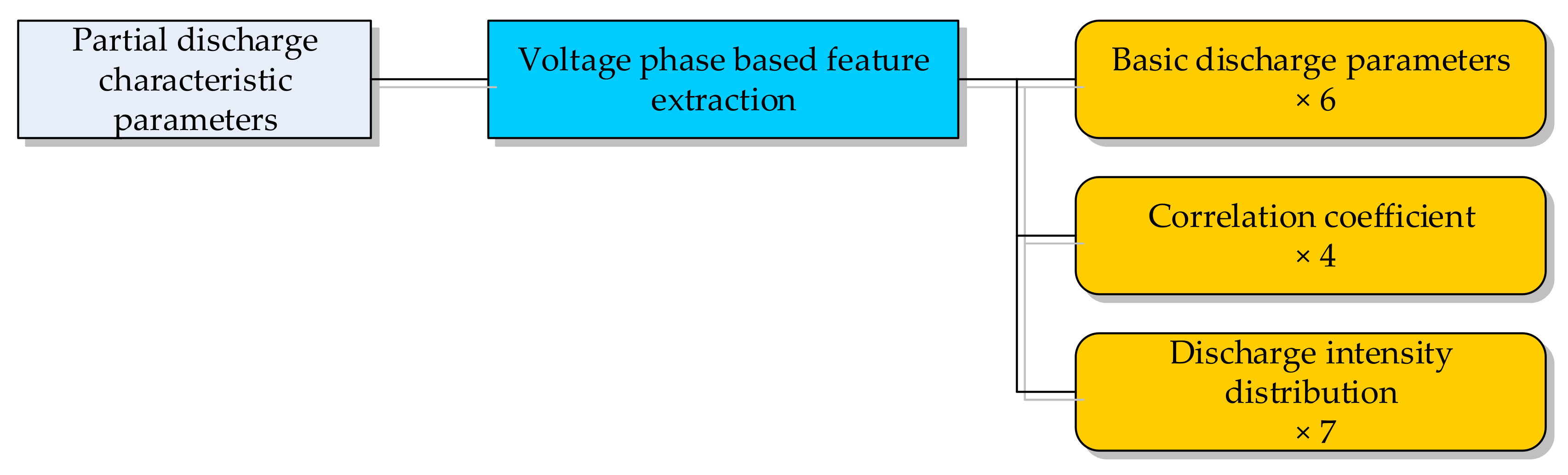
Figure 4.
Features used in this study.
Figure 4.
Features used in this study.
Figure 5.
Selection of features for specific defects.
Figure 5.
Selection of features for specific defects.
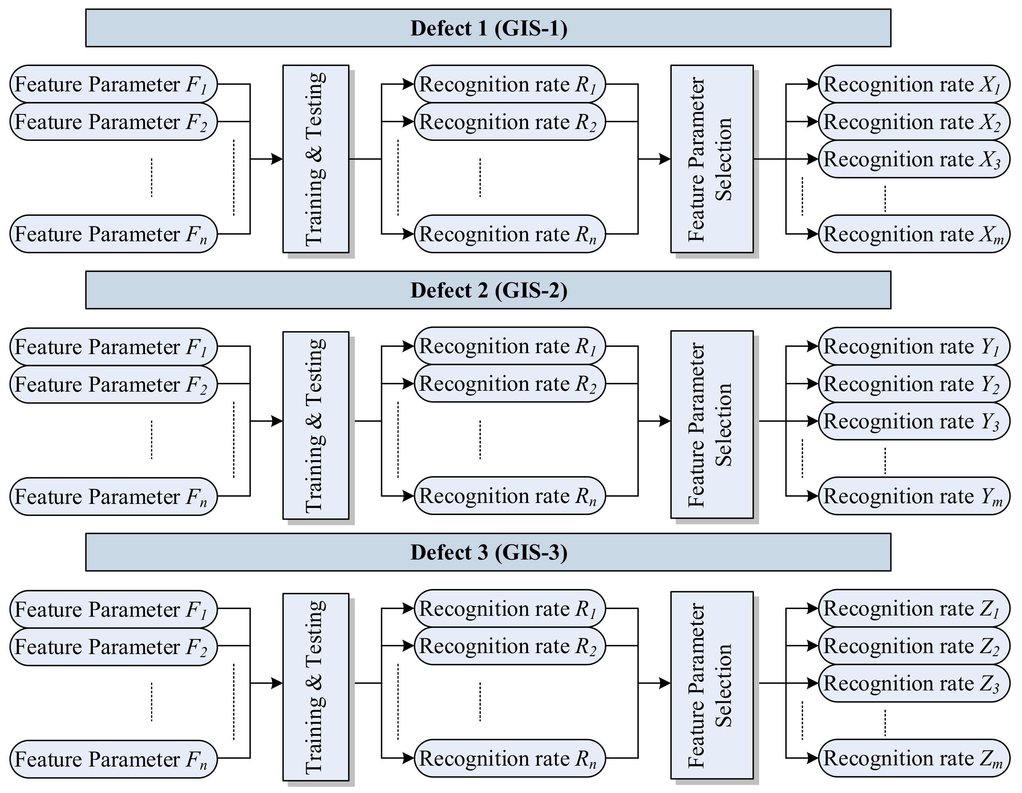
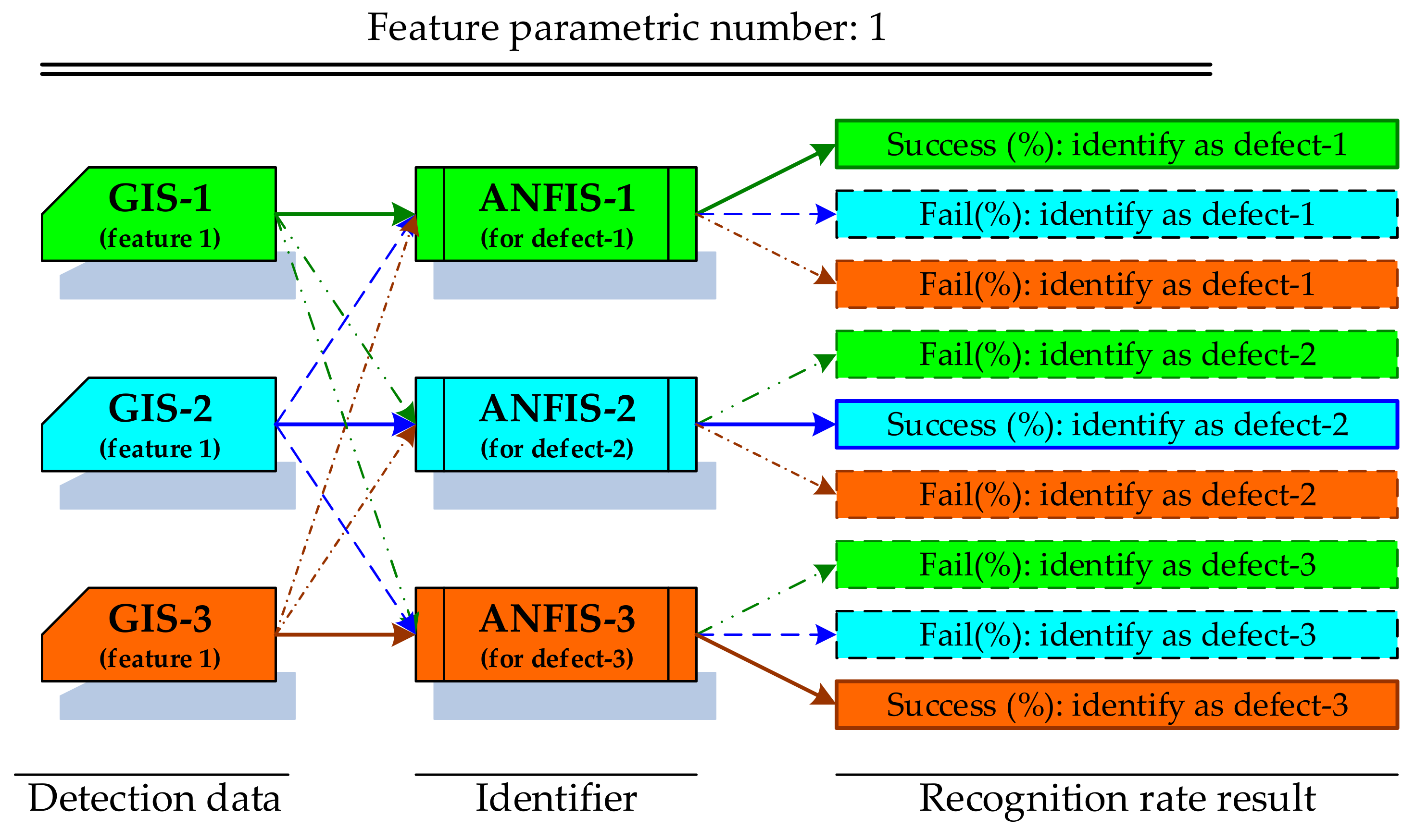
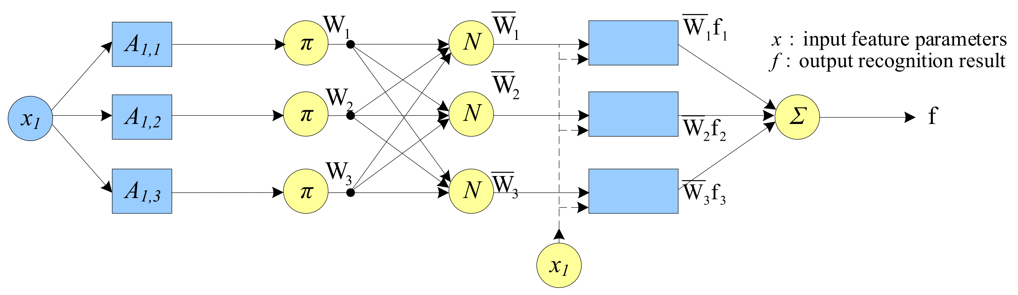
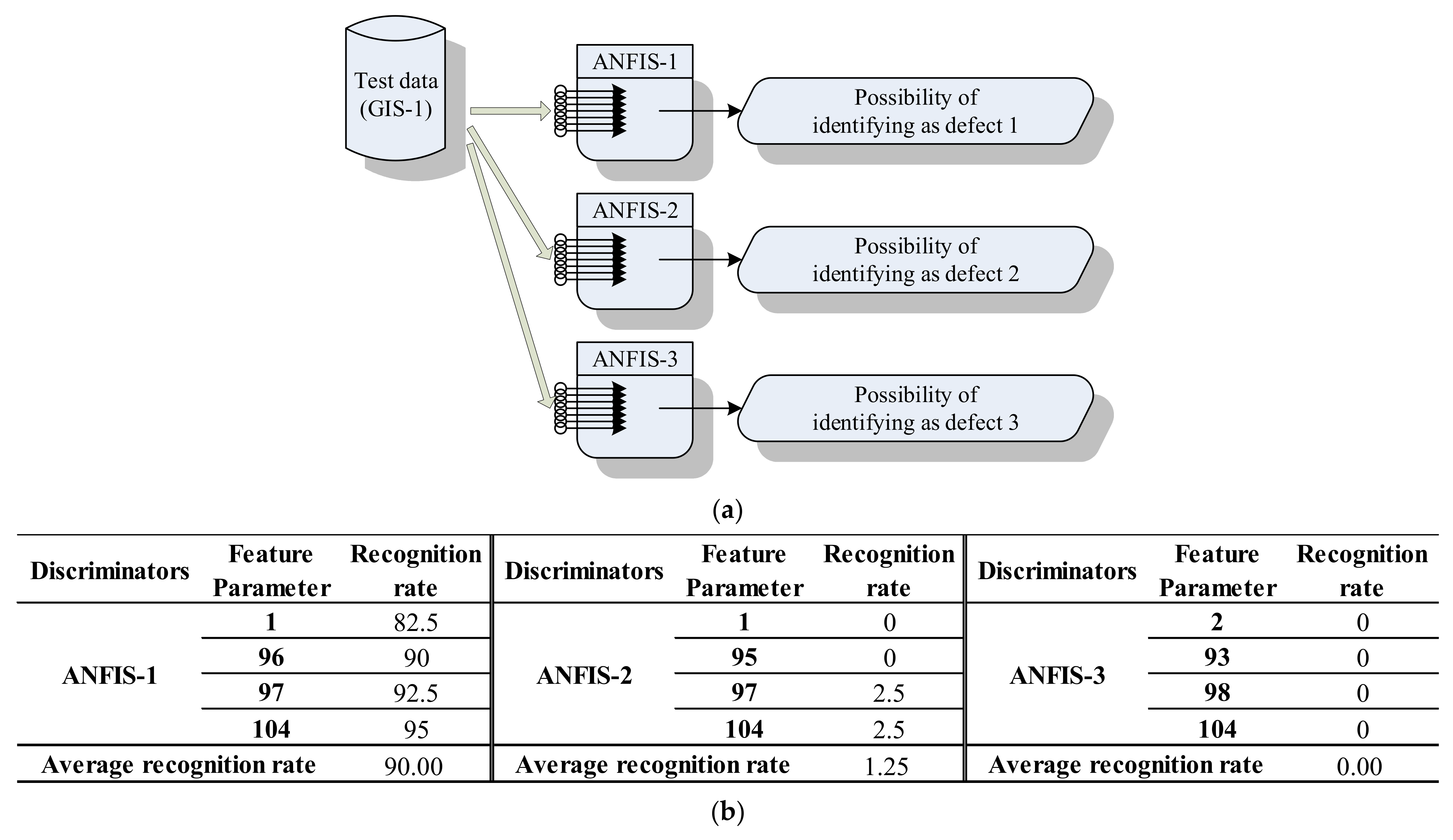
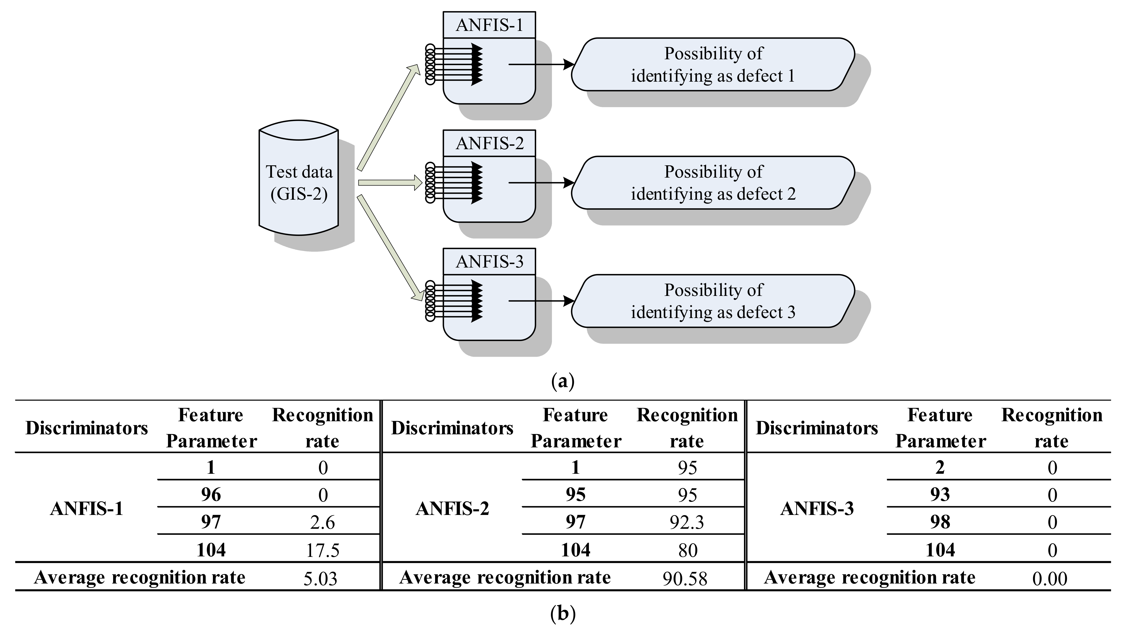
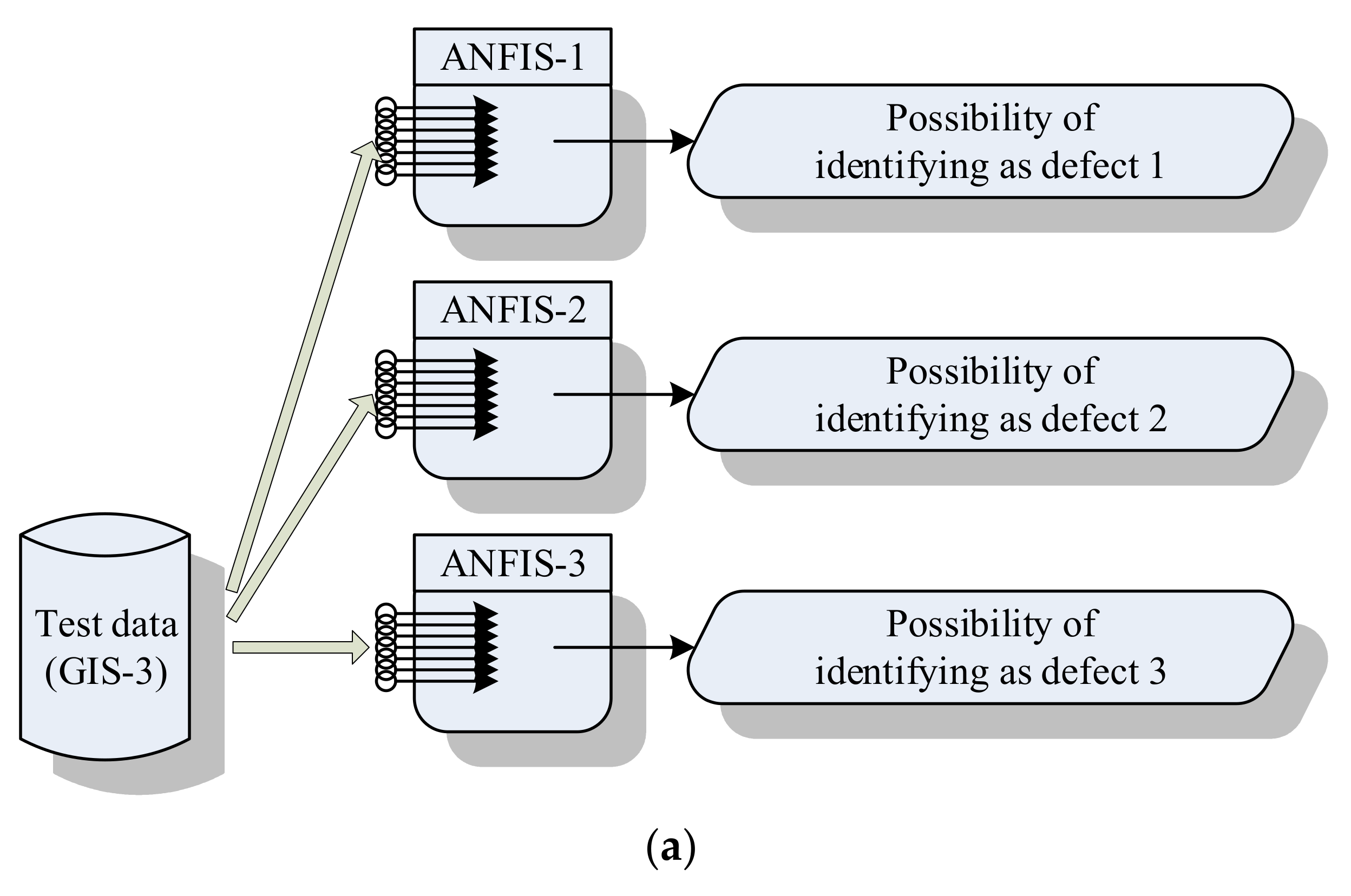
Figure 6.
Schematic diagram of the parallel recognition system.
Figure 6.
Schematic diagram of the parallel recognition system.
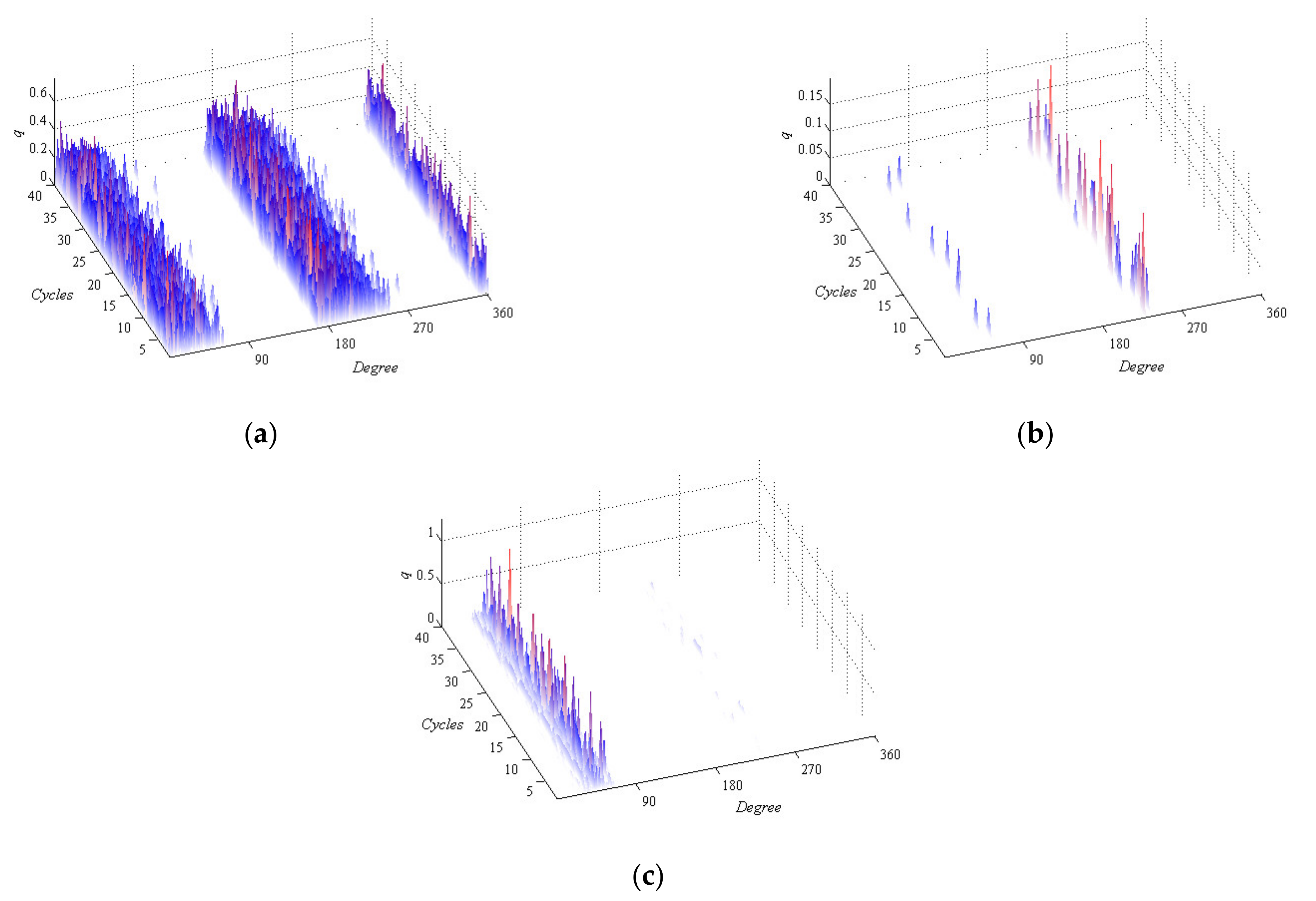
Figure 7.
26 kV patterns: (a) GIS-1; (b) GIS-2; (c) GIS-3.
Figure 7.
26 kV patterns: (a) GIS-1; (b) GIS-2; (c) GIS-3.
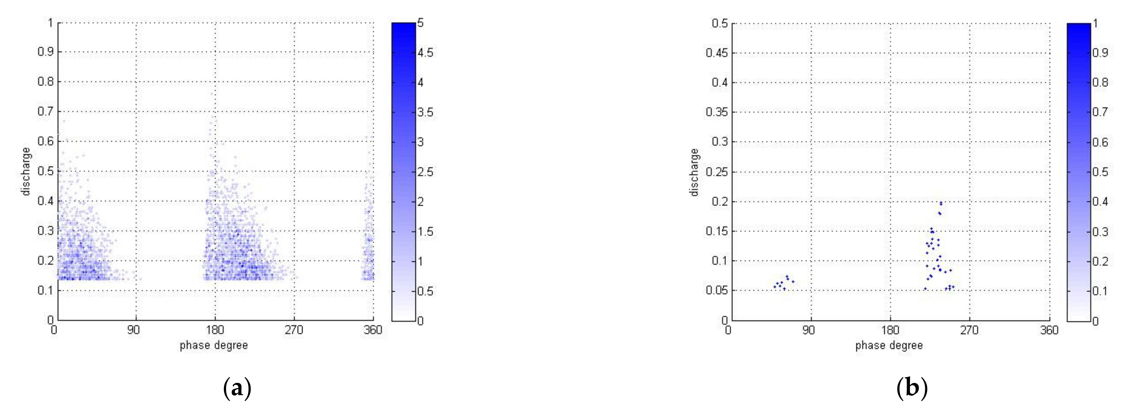
Figure 8.
26 kV patterns: (a) GIS 1; (b) GIS 2; (c) GIS 3.
Figure 8.
26 kV patterns: (a) GIS 1; (b) GIS 2; (c) GIS 3.
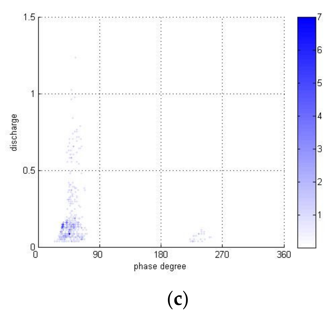
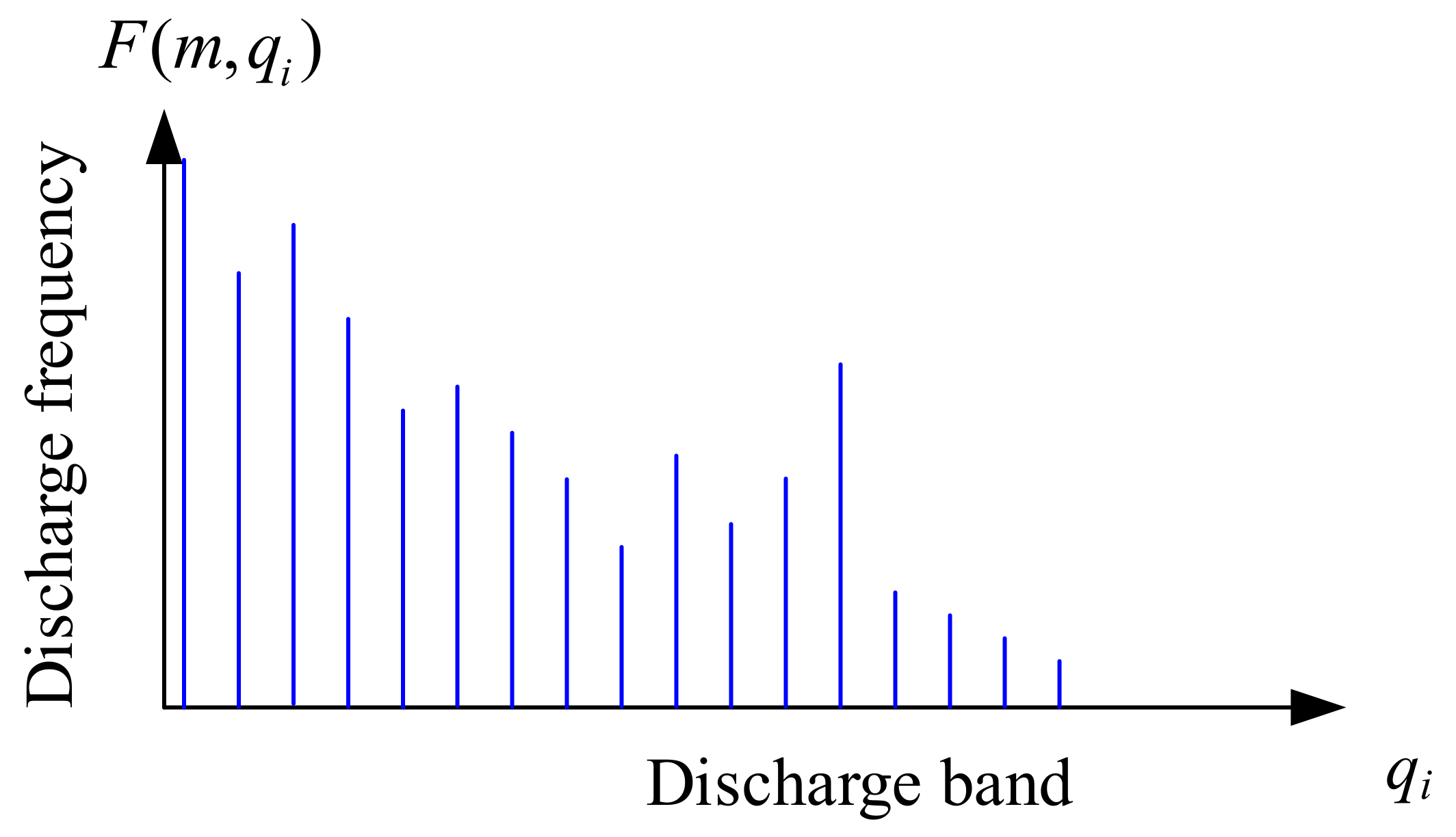
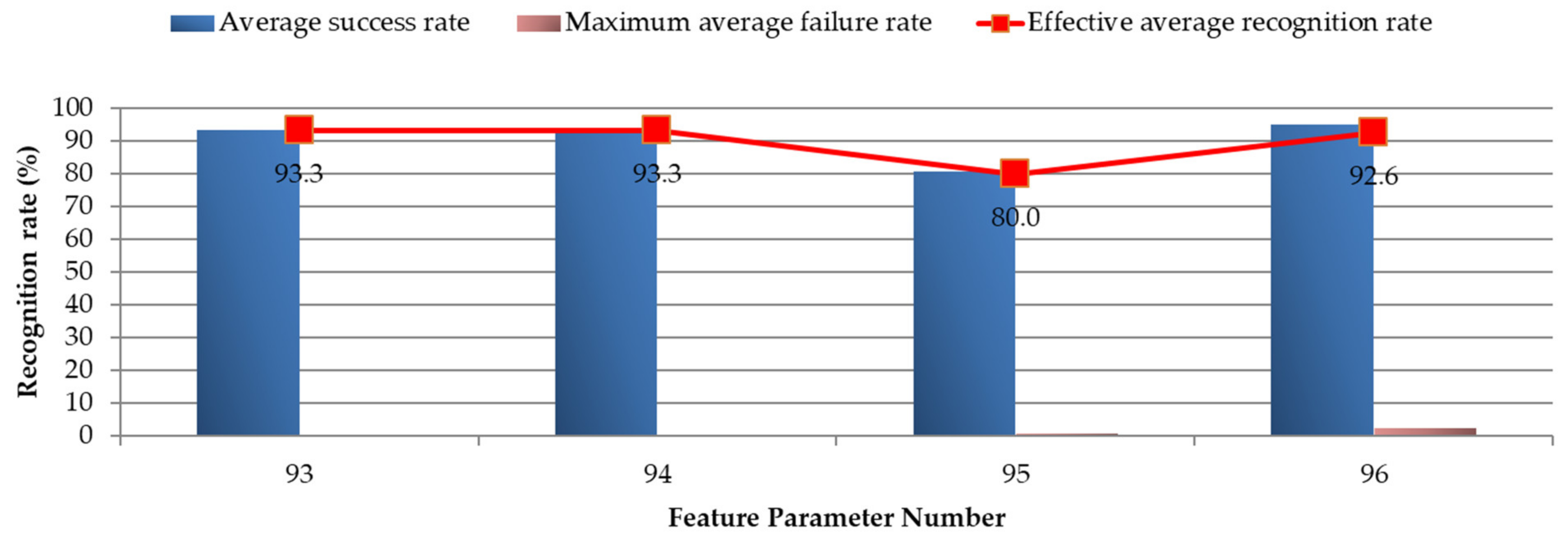
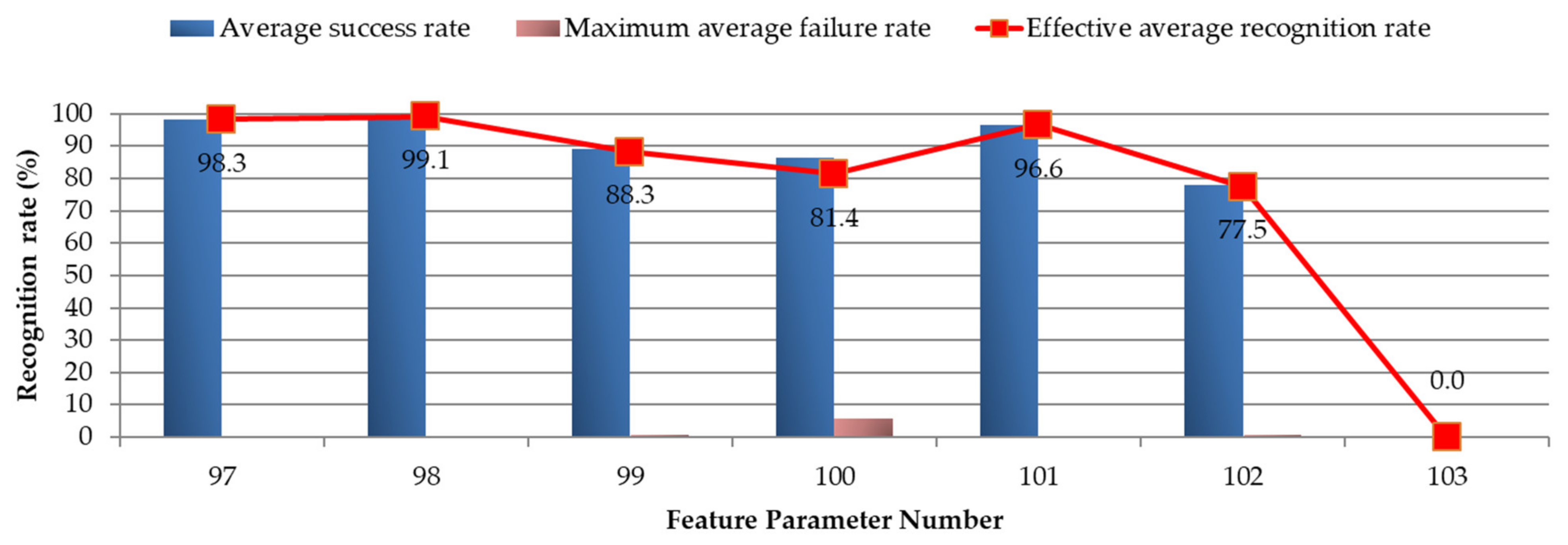
Figure 9.
Schematic diagram of the discharge intensity distribution.
Figure 9.
Schematic diagram of the discharge intensity distribution.
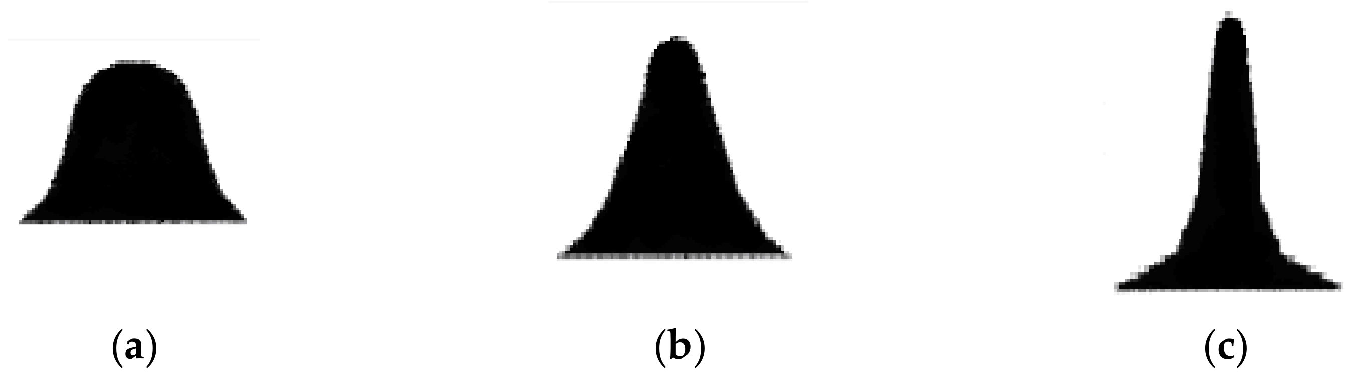
Figure 10.
The shape of the skewed distribution: (a) negative value; (b) equal to zero; (c) positive value.
Figure 10.
The shape of the skewed distribution: (a) negative value; (b) equal to zero; (c) positive value.
Figure 11.
The shape of the kurtosis distribution: (a) negative value; (b) equal to zero; (c) positive value.
Figure 11.
The shape of the kurtosis distribution: (a) negative value; (b) equal to zero; (c) positive value.
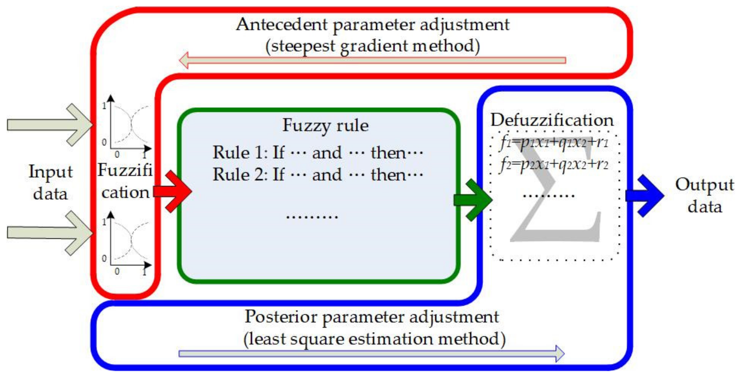
Figure 12.
Schematic diagram of the composite learning process.
Figure 12.
Schematic diagram of the composite learning process.
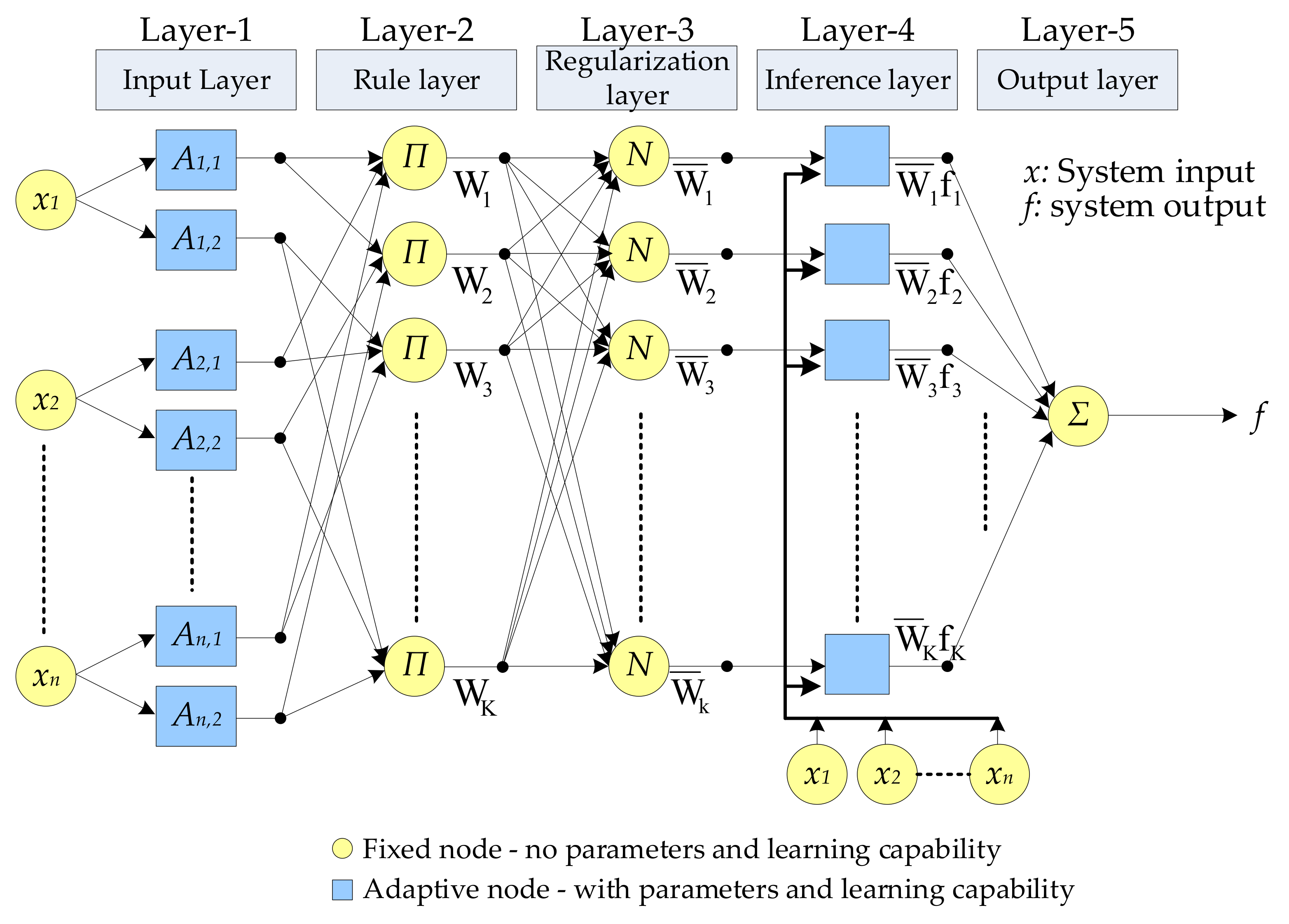
Figure 13.
Schematic of ANFIS architecture (n input, 1 output).
Figure 13.
Schematic of ANFIS architecture (n input, 1 output).
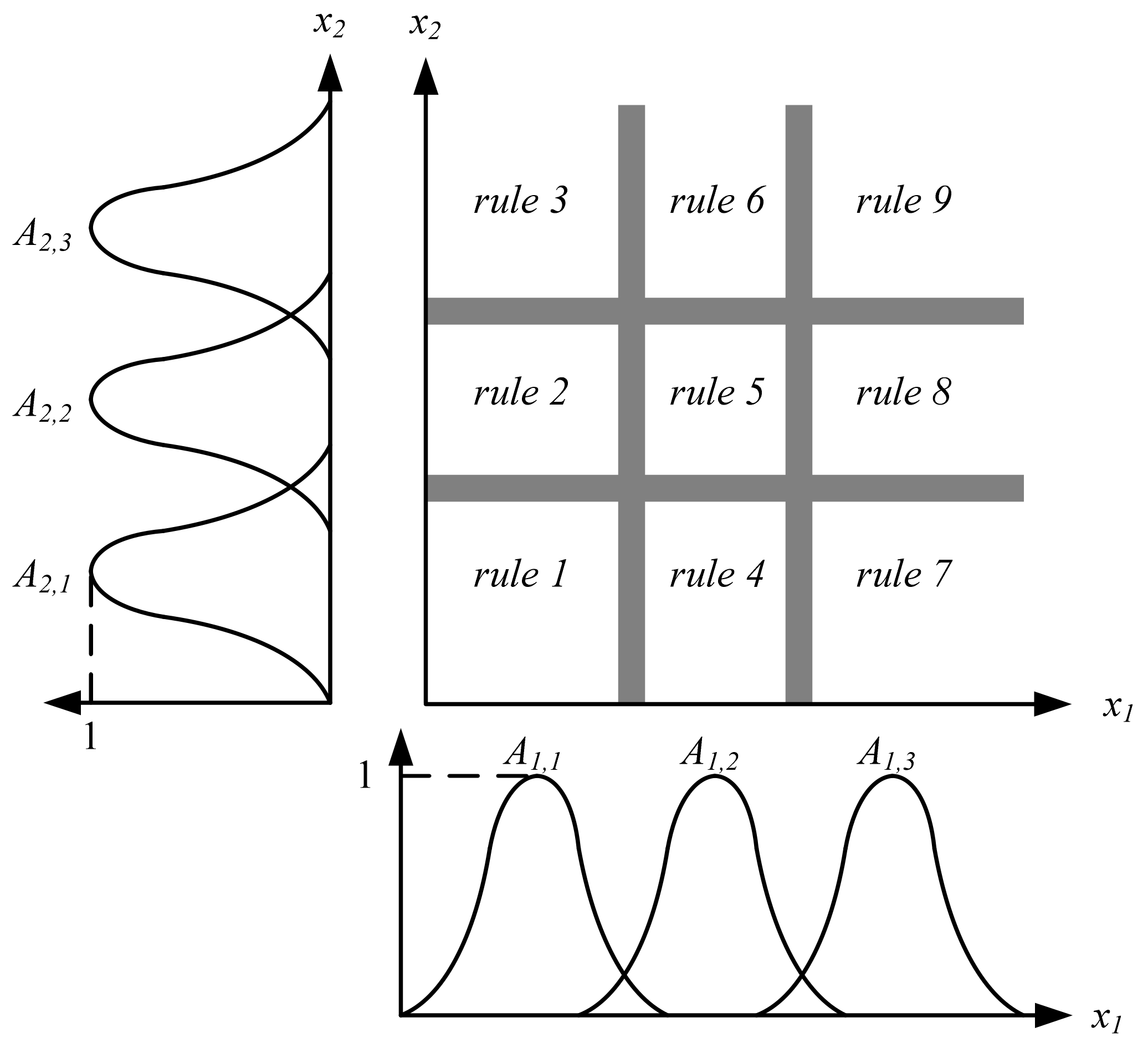
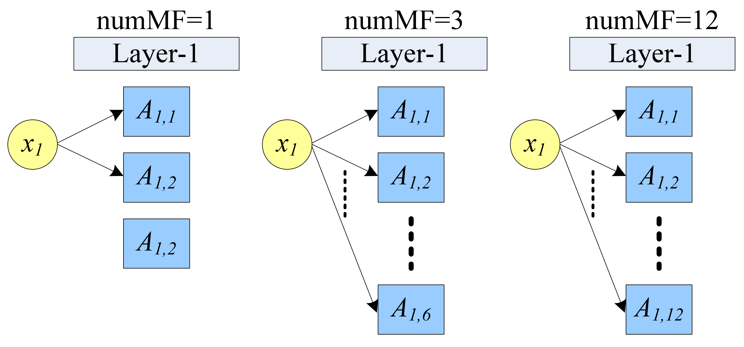
Figure 14.
The input space divided into nine fuzzy sets.
Figure 14.
The input space divided into nine fuzzy sets.
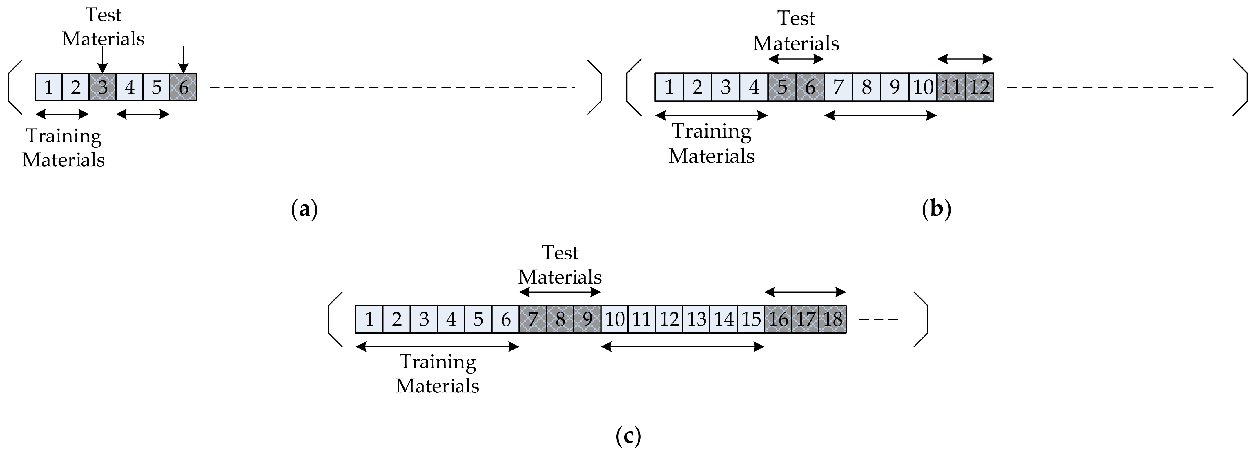
Figure 15.
Schematic diagram of training data and test data architecture: (a) Architecture I: 2/3 are training materials, and 1/3 are test materials; (b) Architecture II: 4/6 for training and 2/6 for testing; (c) Architecture III: 6/9 for training data and 3/9 for testing data.
Figure 15.
Schematic diagram of training data and test data architecture: (a) Architecture I: 2/3 are training materials, and 1/3 are test materials; (b) Architecture II: 4/6 for training and 2/6 for testing; (c) Architecture III: 6/9 for training data and 3/9 for testing data.
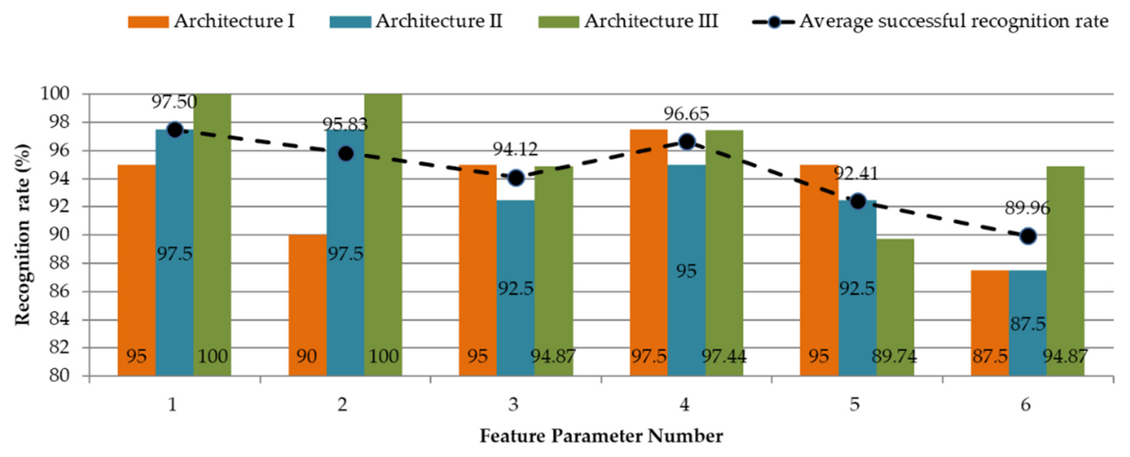
Figure 16.
Analysis of training and test data structure.
Figure 16.
Analysis of training and test data structure.
Figure 17.
Discriminator training flow.
Figure 17.
Discriminator training flow.
Figure 18.
System architecture for testing attributable function types.
Figure 18.
System architecture for testing attributable function types.
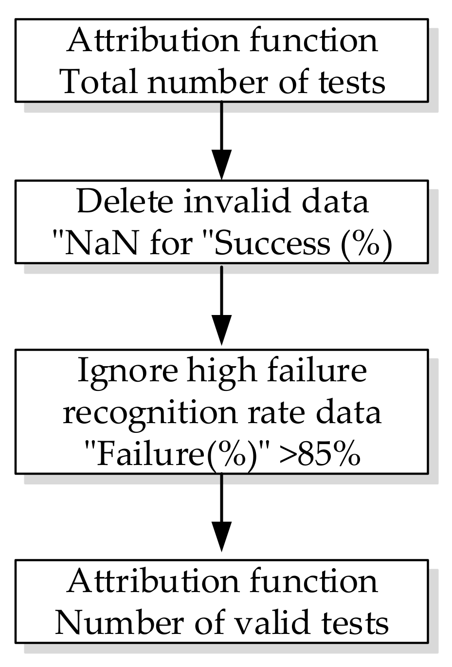
Figure 19.
Data filtering process for attribution functions.
Figure 19.
Data filtering process for attribution functions.
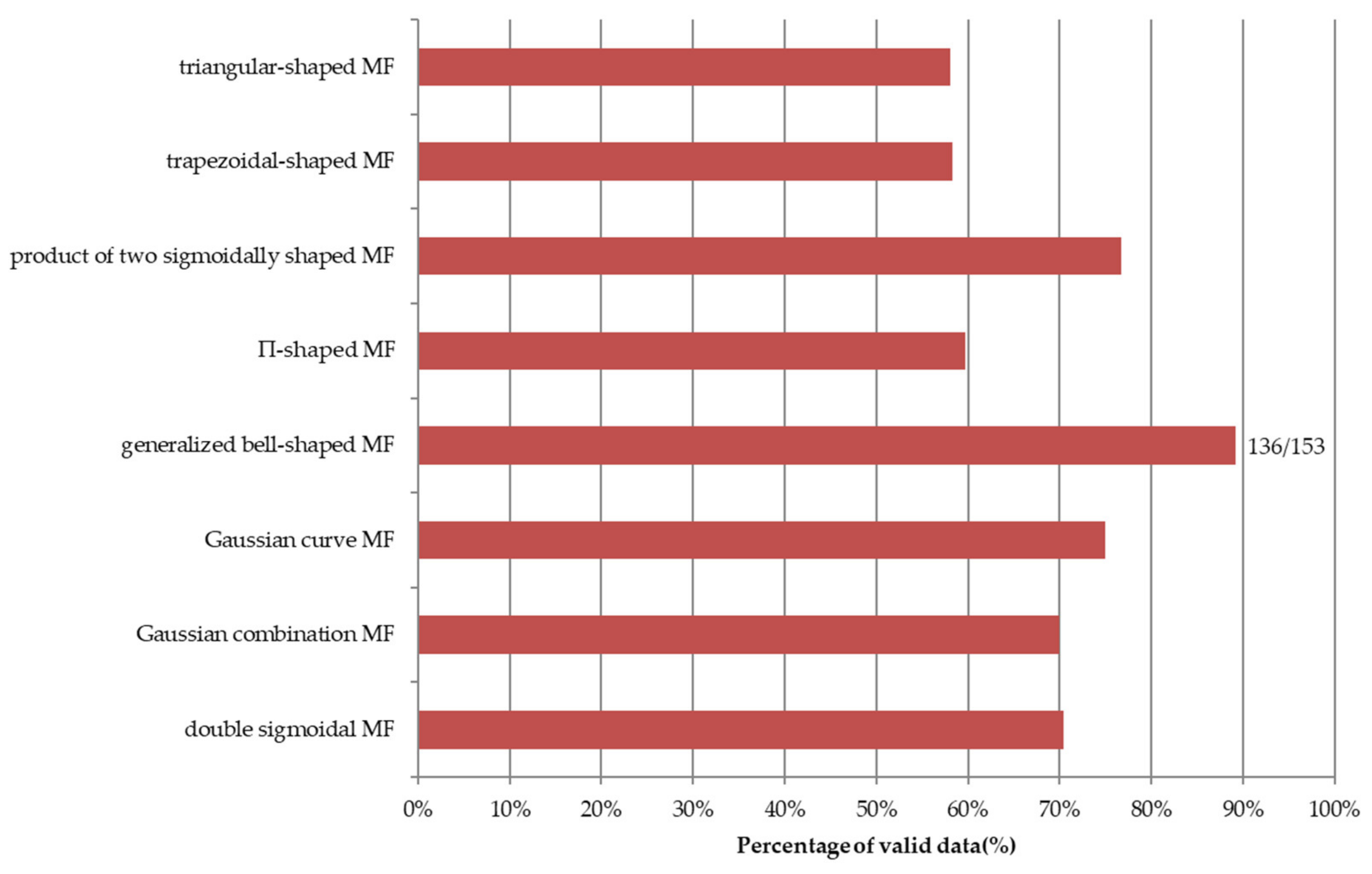
Figure 20.
Percentage of valid data for each attribution function.
Figure 20.
Percentage of valid data for each attribution function.
Figure 21.
Diagram of different attribution functions in the ANFIS architecture.
Figure 21.
Diagram of different attribution functions in the ANFIS architecture.
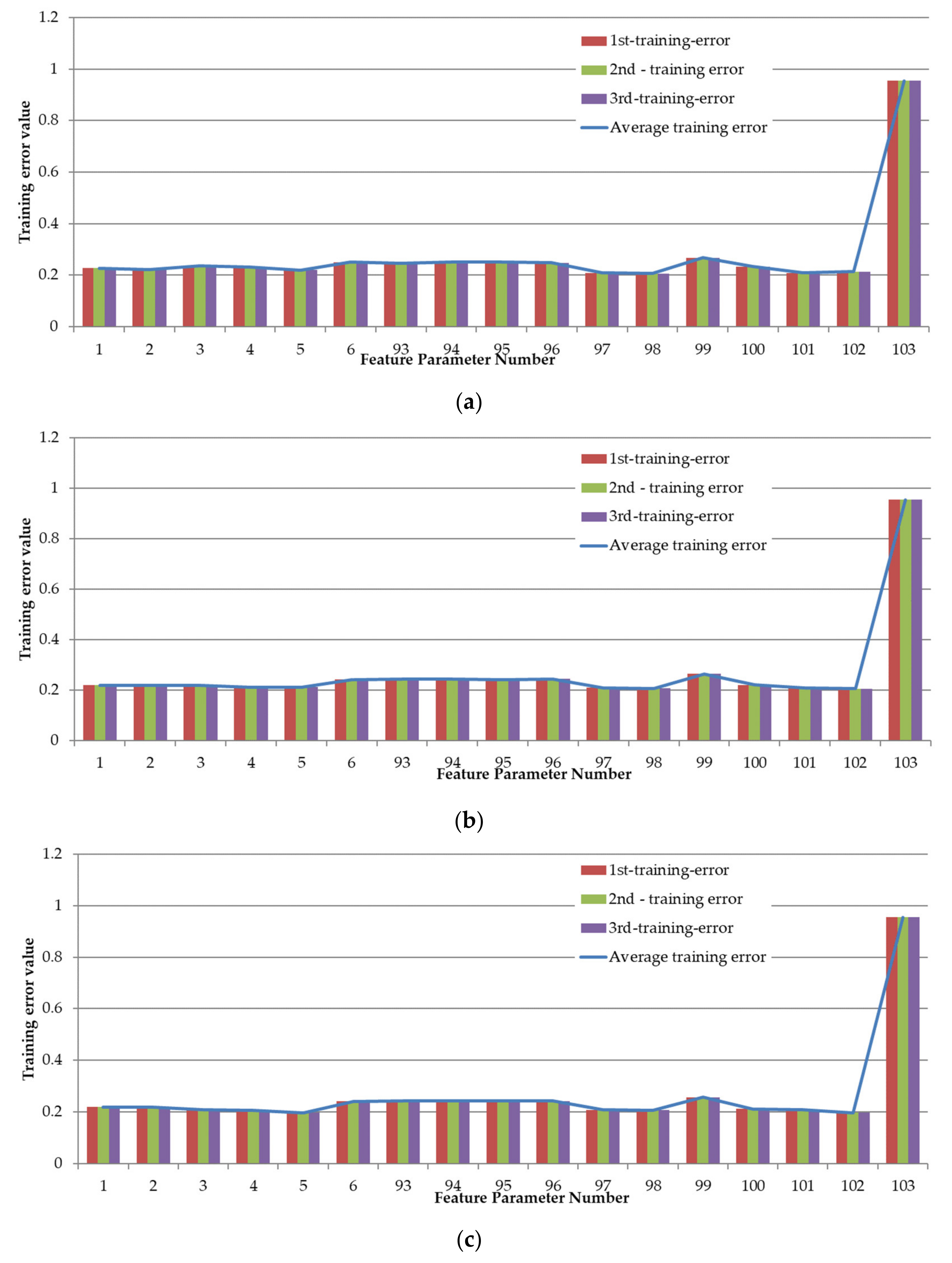
Figure 22.
Training error for different MFs: (a) Test 1: numMF = 3; (b) Test 2: numMF = 6; (c) Test 3: numMF = 12.
Figure 22.
Training error for different MFs: (a) Test 1: numMF = 3; (b) Test 2: numMF = 6; (c) Test 3: numMF = 12.
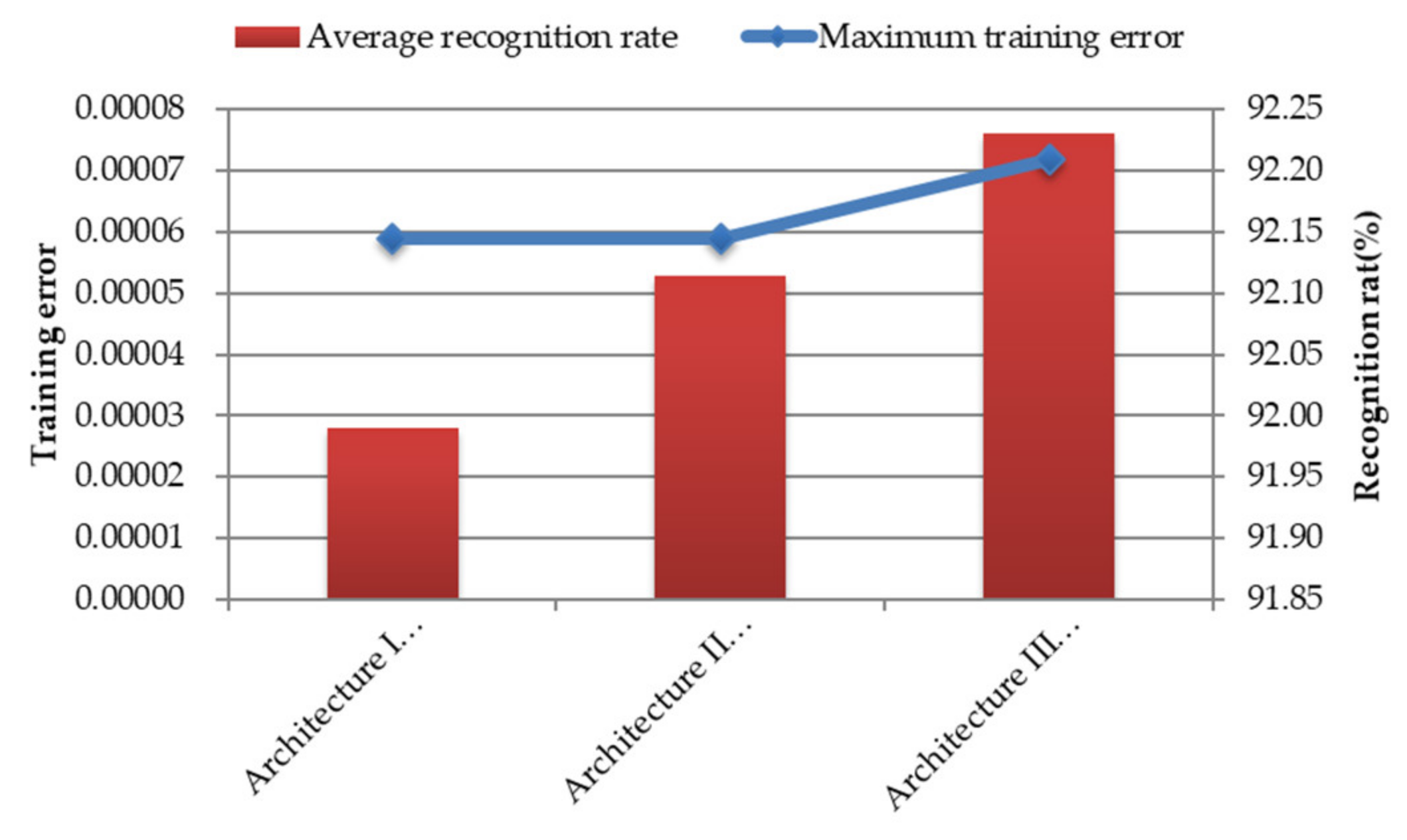
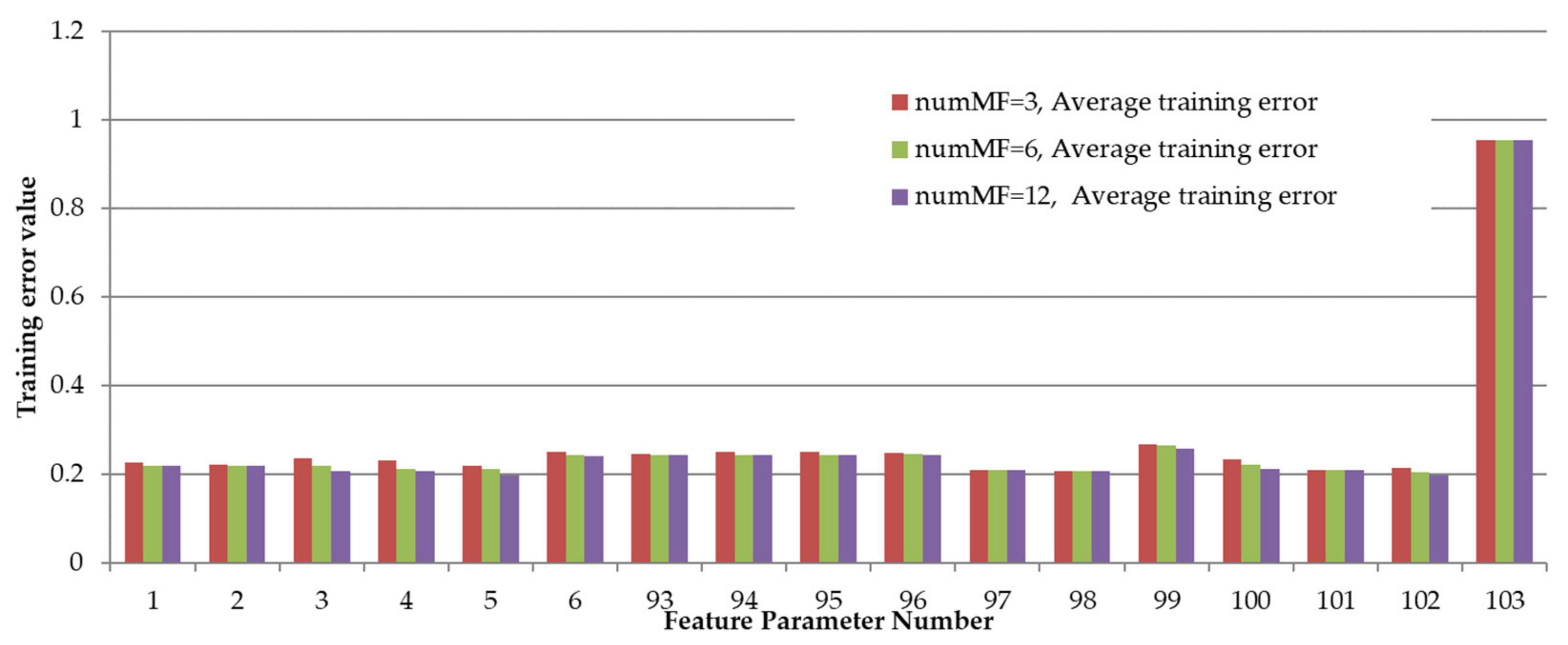
Figure 23.
Average training error for different MFs.
Figure 23.
Average training error for different MFs.
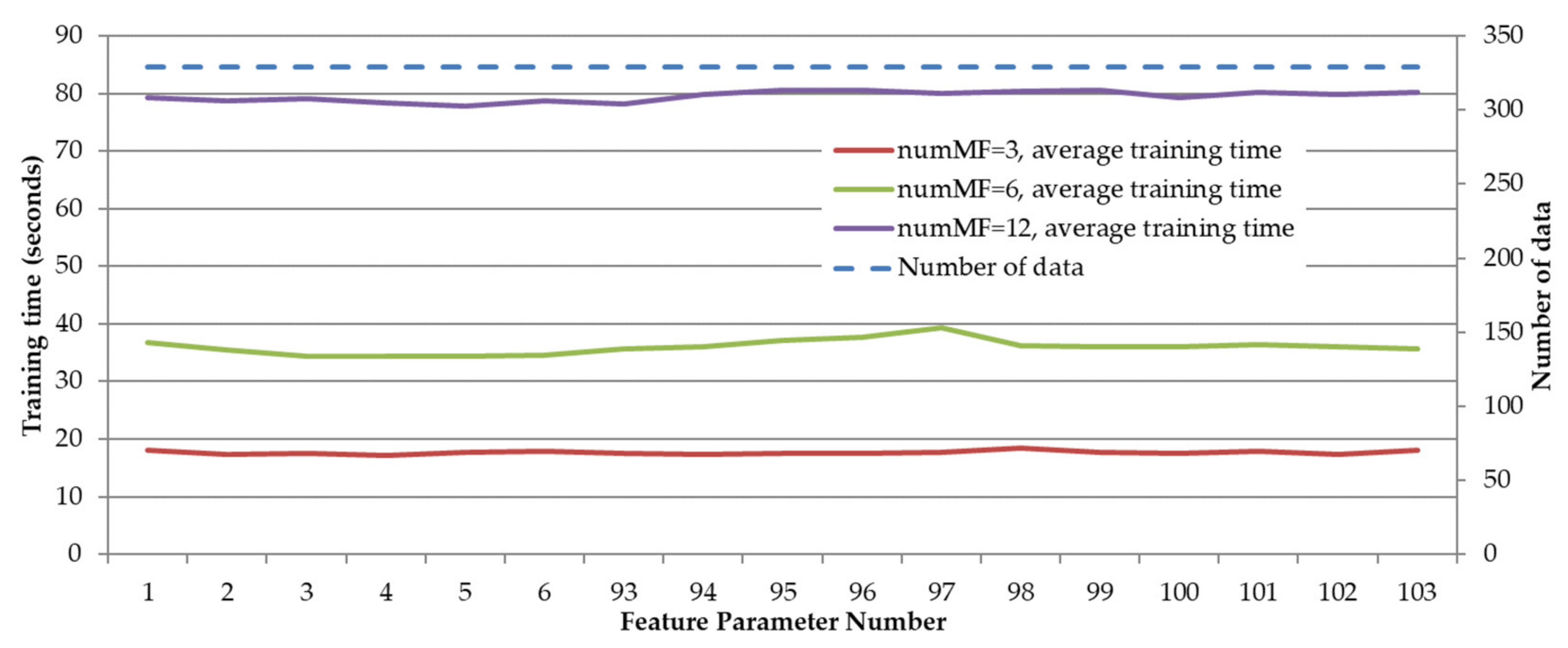
Figure 24.
Average training time for different MFs.
Figure 24.
Average training time for different MFs.
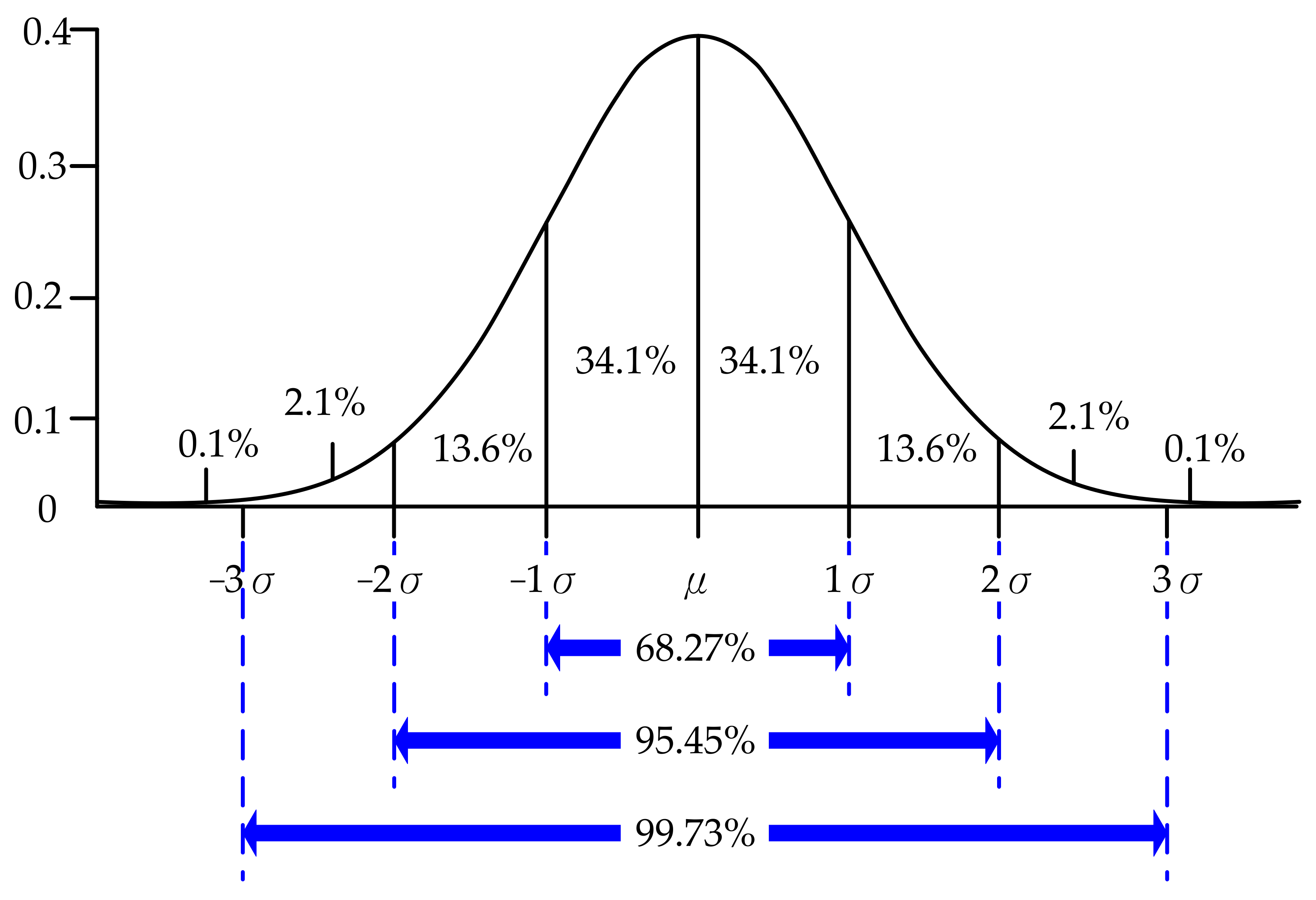
Figure 25.
Rules for the mean and standard deviation in normally distributed data.
Figure 25.
Rules for the mean and standard deviation in normally distributed data.
Figure 26.
Standard deviation–recognition rate curve for the recognition threshold. (a) Defect type 1 (take Feature-1 as an example). (b) Defect type 2 (take Feature-93 as an example). (c) Defect type 3 (take Feature-97 as an example).
Figure 26.
Standard deviation–recognition rate curve for the recognition threshold. (a) Defect type 1 (take Feature-1 as an example). (b) Defect type 2 (take Feature-93 as an example). (c) Defect type 3 (take Feature-97 as an example).
Figure 27.
Schematic diagram of ANFIS architecture for partial discharge defect classification.
Figure 27.
Schematic diagram of ANFIS architecture for partial discharge defect classification.
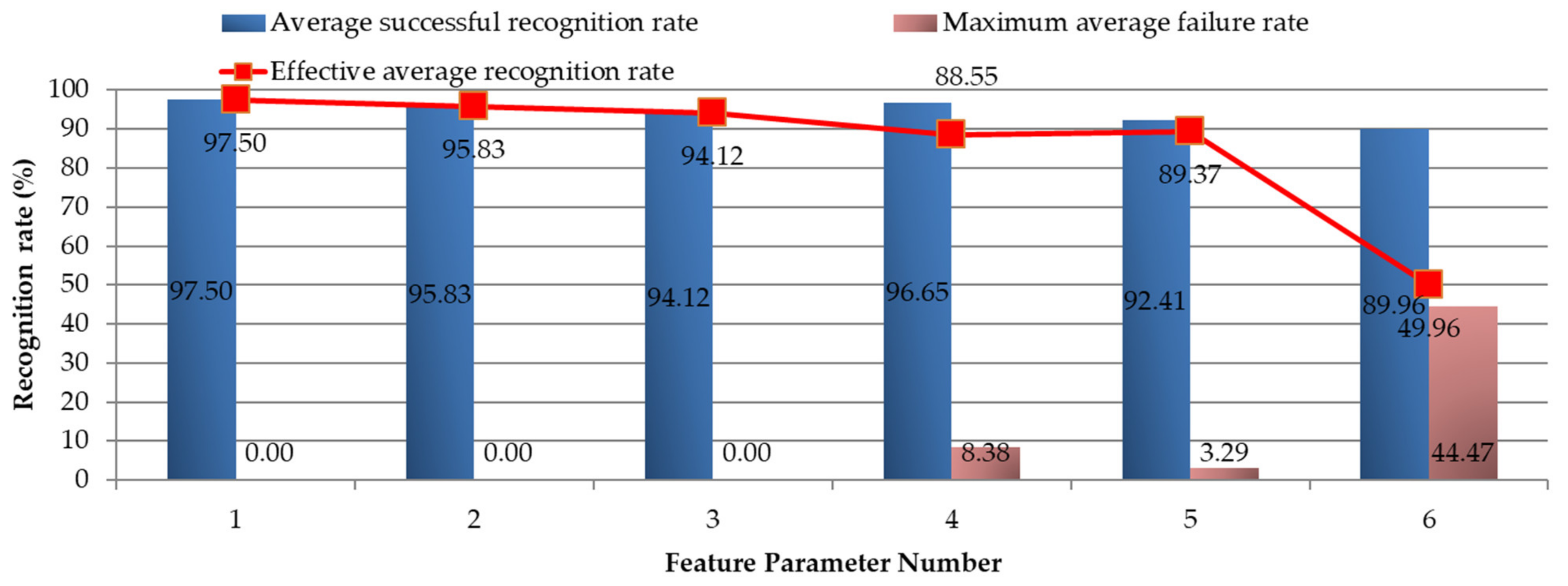
Figure 28.
The successful recognition rate of each architecture (GIS-2).
Figure 28.
The successful recognition rate of each architecture (GIS-2).
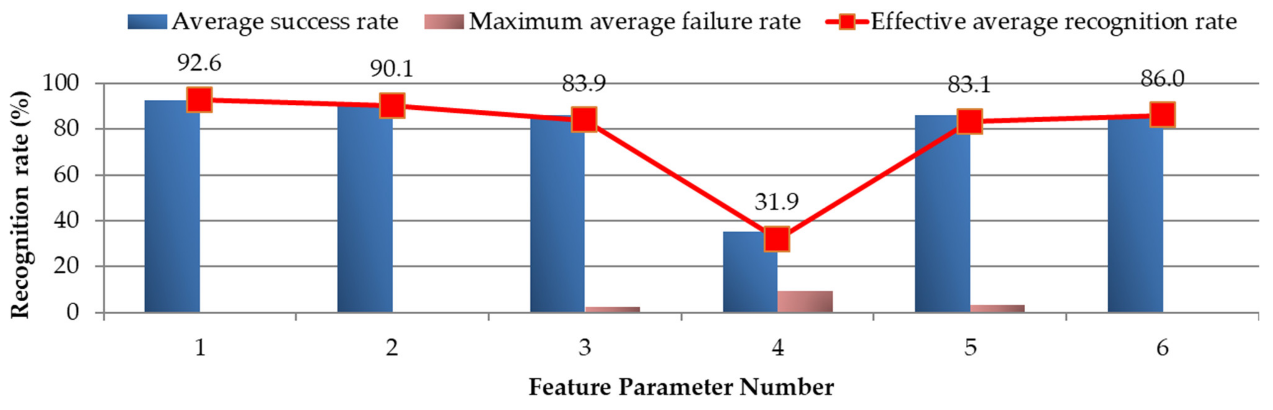
Figure 29.
The effective average recognition rate.
Figure 29.
The effective average recognition rate.
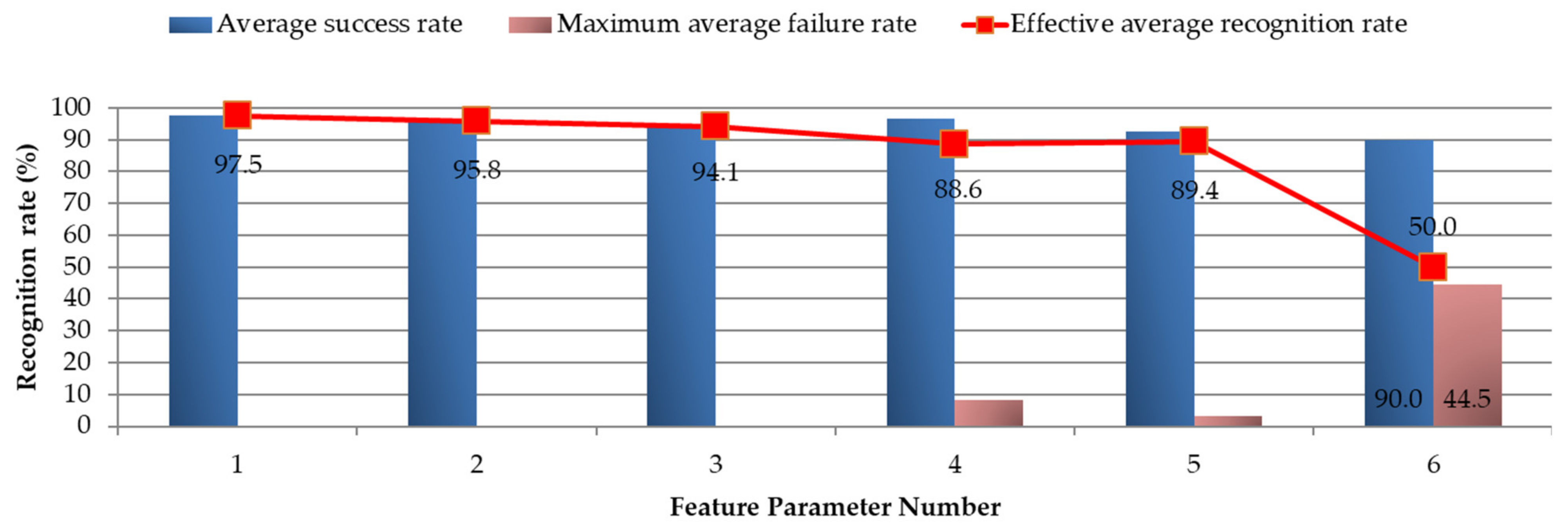
Figure 30.
GIS-1 partial discharge feature: basic discharge parameter recognition rate.
Figure 30.
GIS-1 partial discharge feature: basic discharge parameter recognition rate.
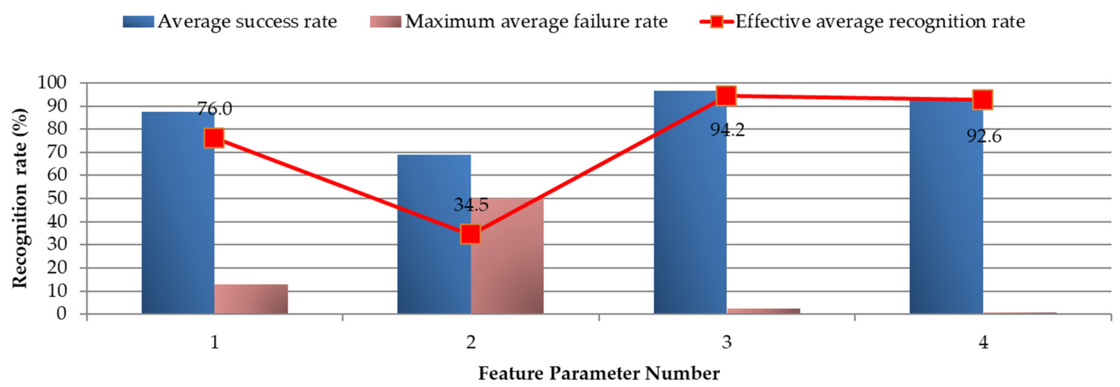
Figure 31.
GIS-1 partial discharge parameter: cross-correlation coefficient recognition rate.
Figure 31.
GIS-1 partial discharge parameter: cross-correlation coefficient recognition rate.
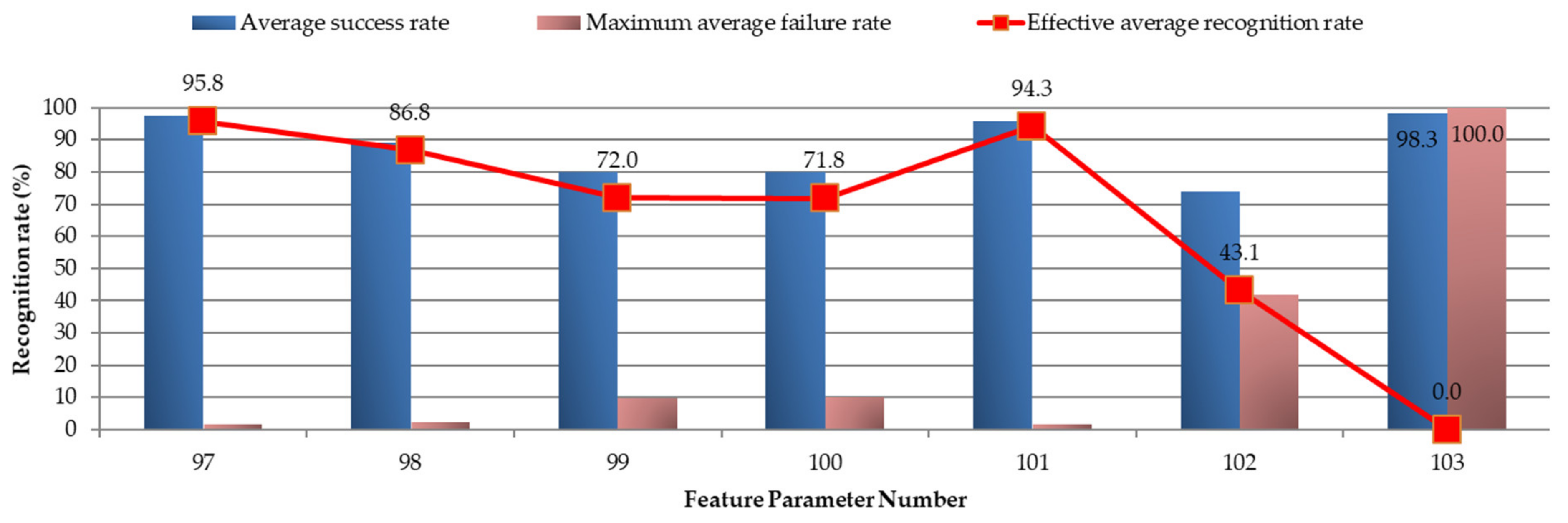
Figure 32.
GIS-1 partial discharge characteristics: discharge strength distribution recognition rate.
Figure 32.
GIS-1 partial discharge characteristics: discharge strength distribution recognition rate.
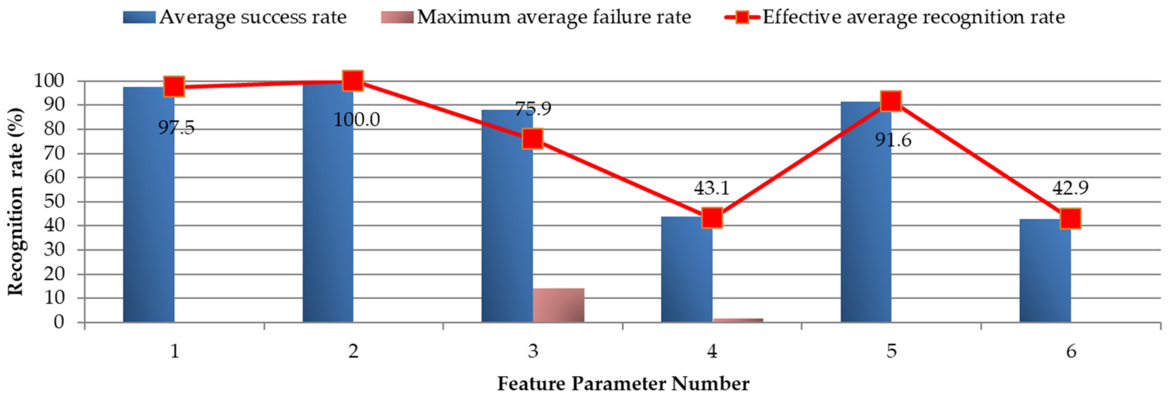
Figure 33.
GIS-2 partial discharge parameter: basic discharge parameter recognition rate.
Figure 33.
GIS-2 partial discharge parameter: basic discharge parameter recognition rate.
Figure 34.
GIS-2 Partial discharge parametric: cross-correlation coefficient recognition rate.
Figure 34.
GIS-2 Partial discharge parametric: cross-correlation coefficient recognition rate.
Figure 35.
GIS-2 partial discharge characteristic parameter: discharge intensity distribution recognition rate.
Figure 35.
GIS-2 partial discharge characteristic parameter: discharge intensity distribution recognition rate.
Figure 36.
GIS-3 partial discharge parameter: basic discharge parameter recognition rate.
Figure 36.
GIS-3 partial discharge parameter: basic discharge parameter recognition rate.
Figure 37.
GIS-3 partial discharge parametric: cross-correlation coefficient recognition rate.
Figure 37.
GIS-3 partial discharge parametric: cross-correlation coefficient recognition rate.
Figure 38.
GIS-3 partial discharge characteristic parameters: identification rate of the discharge intensity distribution.
Figure 38.
GIS-3 partial discharge characteristic parameters: identification rate of the discharge intensity distribution.
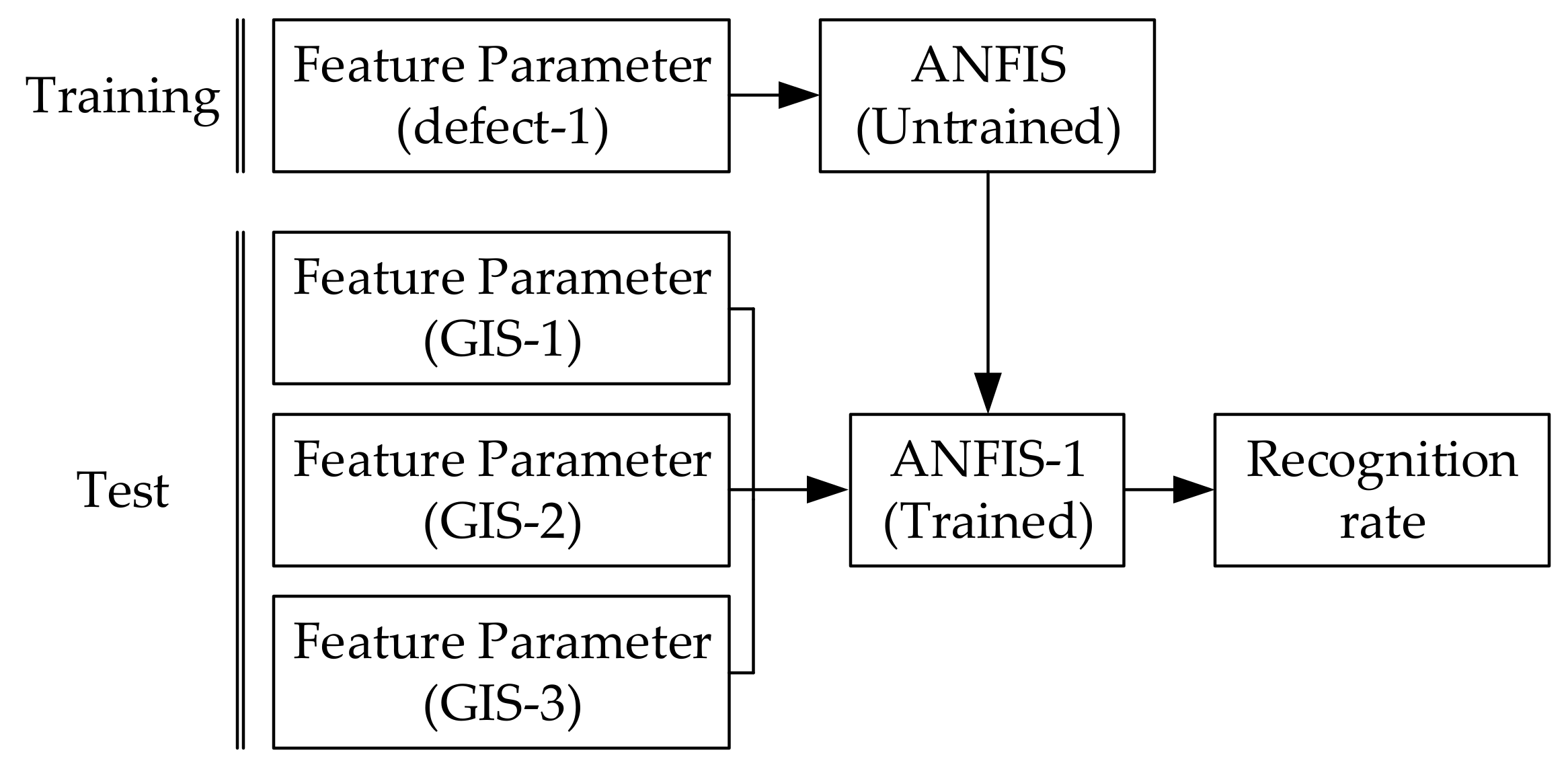
Figure 39.
GIS-1 in parallel recognition system: (a) test architecture; (b) test results.
Figure 39.
GIS-1 in parallel recognition system: (a) test architecture; (b) test results.
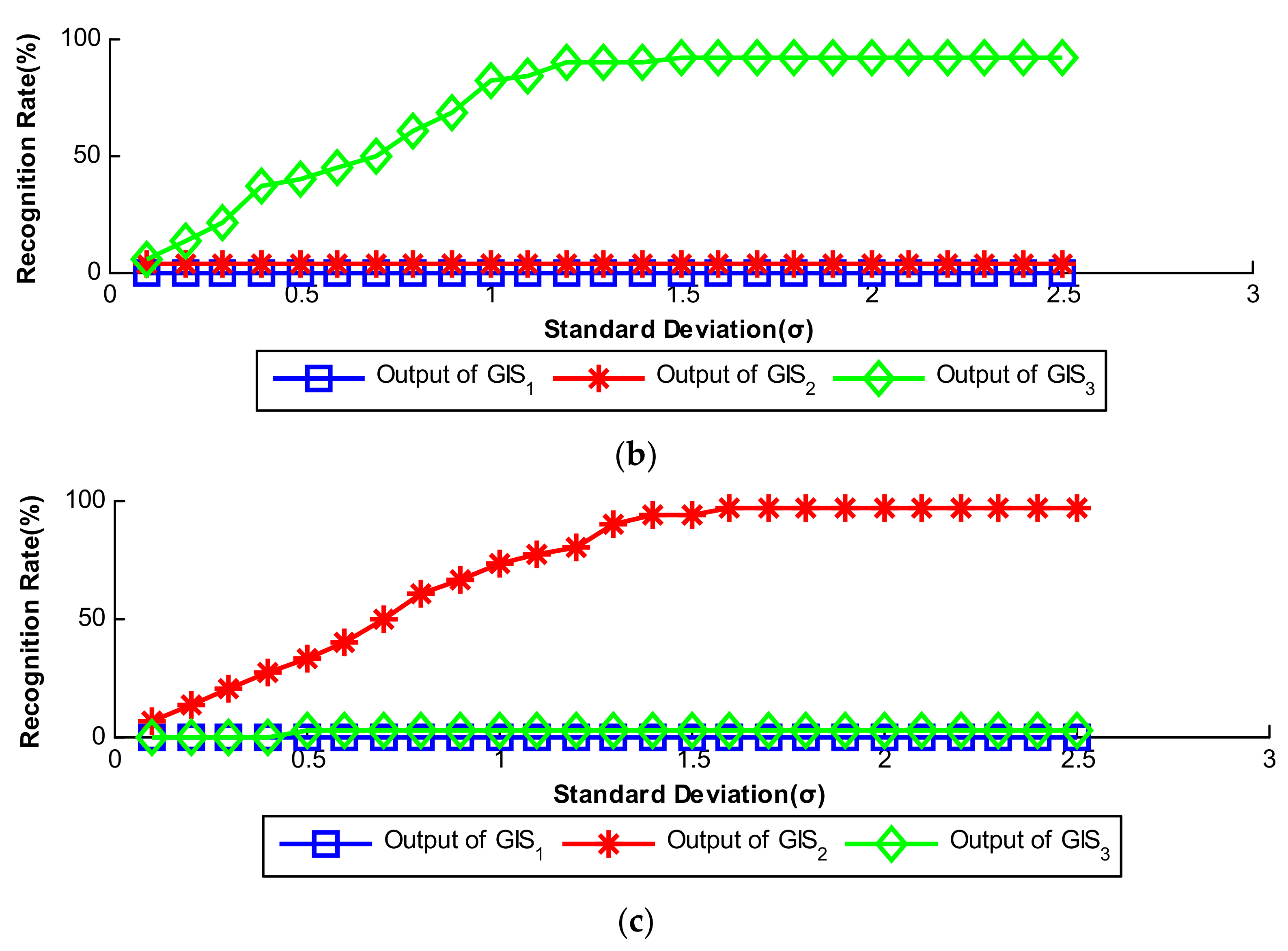
Figure 40.
GIS-2 in parallel recognition system: (a) test architecture; (b) test results.
Figure 40.
GIS-2 in parallel recognition system: (a) test architecture; (b) test results.
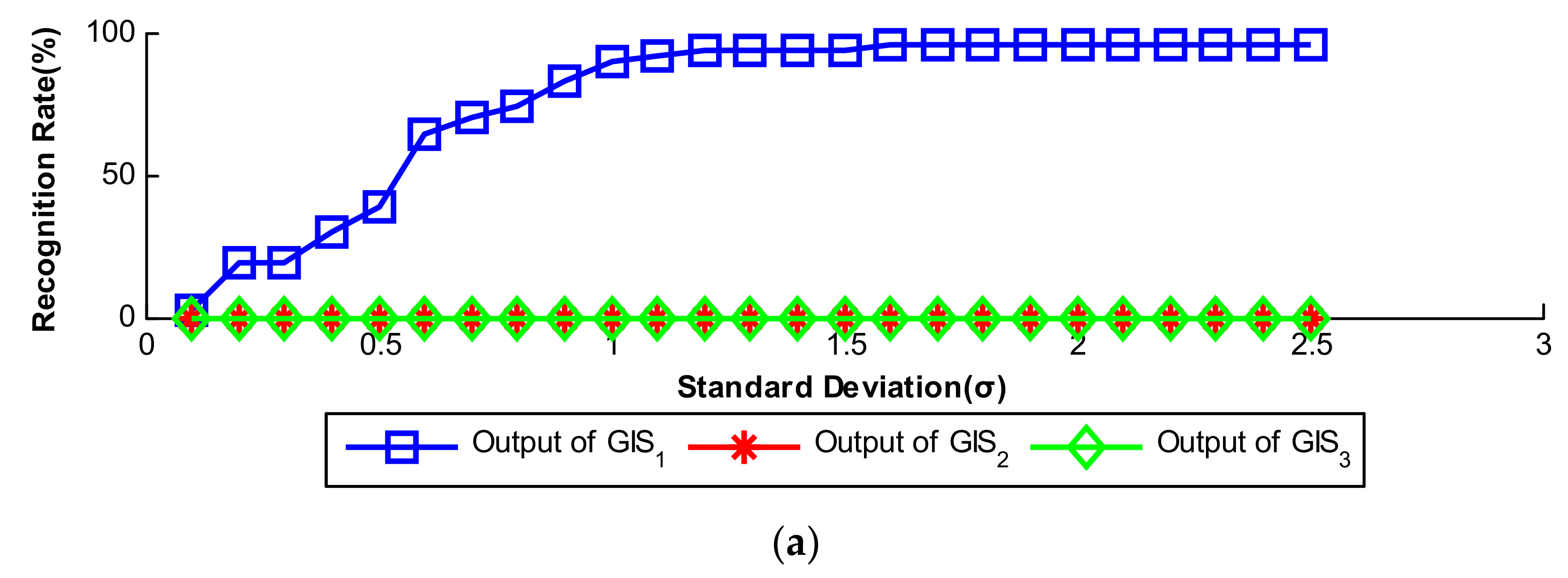
Figure 41.
GIS-3 in parallel recognition system: (a) test architecture; (b) test results.
Figure 41.
GIS-3 in parallel recognition system: (a) test architecture; (b) test results.
Table 1.
Partial discharge characteristic parameters: basic discharge parameters.
Table 1.
Partial discharge characteristic parameters: basic discharge parameters.
| No. | Program Code | Description |
|---|
| 1 | Q-All Cycle-Quantity Height-Sum | Total number of discharges in the whole cycle |
| 2 | Q-All Cycle-Quantity Height-Num | The number of discharges in the whole cycle |
| 3 | Q-All Cycle-Quantity Height-Ave | Average discharge volume of the whole cycle |
| 4 | Q-All Cycle-Quantity Height-Max | Maximum discharge volume of the whole cycle |
| 5 | Q-All Cycle-Quantity Height-Med | Median discharge volume of the whole cycle |
| 6 | Q-All Cycle-Quantity Height-Mod | Plurality of discharges for the whole cycle |
Table 2.
Partial discharge characteristic parameters: modified cross-correlation factor.
Table 2.
Partial discharge characteristic parameters: modified cross-correlation factor.
| No. | Program Code | Description |
|---|
| 93 | Q- All Cycle-CC-Sum | Correlation coefficient between the sum of positive and negative half-cycle discharges and phase |
| 94 | Q- All Cycle-CC-Num | Number of discharges in positive and negative half-weeks - phase correlation coefficient |
| 95 | Q- All Cycle-CC-Ave | Average discharge volume of positive and negative half-weeks - phase correlation coefficient |
| 96 | Q- All Cycle-CC-Max | Maximum discharge volume of positive and negative half-weeks - phase correlation coefficient |
Table 3.
Partial discharge characteristic parameters: discharge intensity distribution.
Table 3.
Partial discharge characteristic parameters: discharge intensity distribution.
| No. | Program Code | Description |
|---|
| 97 | Q- All Cycle-Intensity freq_mu | Average value of discharge intensity |
| 98 | Q- All Cycle-Intensity freq_std | Standard Deviation of Discharge Intensity |
| 99 | Q- All Cycle-Intensity freq_sk | Bias of discharge intensity |
| 100 | Q- All Cycle-Intensity freq_ku | Peak state of discharge intensity |
| 101 | Q- All Cycle-Intensity freq_WblScale | Weber Scale of Discharge Intensity |
| 102 | Q- All Cycle-Intensity freq_WblShape | Weber shape parameter of discharge intensity |
| 103 | Q- All Cycle-Intensity freq_KStest | Weber calibration value of discharge intensity |
Table 4.
The compound learning program approach.
Table 4.
The compound learning program approach.
| | Forward Pass | Backward Pass |
|---|
| premise parameters | fixed | gradient descent |
| consequent parameters | least-square estimator | fixed |
| signals | node output | error signal |
Table 5.
Basic ANFIS setup information.
Table 5.
Basic ANFIS setup information.
| | Test 1 | Test 2 | Test 3 |
|---|
| MF(Layer-1): | generalized bell | generalized bell | generalized bell |
| numMF: | 3 | 6 | 12 |
| T-norm(Layer-2) | product | product | product |
| Output(Layer-5) | Weighted average | Weighted average | Weighted average |
Table 6.
ANFIS training setup items.
Table 6.
ANFIS training setup items.
| Name | Item |
|---|
| Number of training samples | 360 (26 kV) |
| Number of training epochs | 1000 (epochs) |
| Operation method measurement | T-normMax-product |
| Optimization method | Hybrid |
| Attribution function MF | generalized bell |
| Number of functions numMF | 3 |
Table 7.
GIS-1 better recognition rate of characteristic parameters: basic discharge parameters.
Table 7.
GIS-1 better recognition rate of characteristic parameters: basic discharge parameters.
| Feature Parameters | RECAS | RECF | RECEA |
|---|
| No. | Name | Average Success Rate | Maximum Average Failure Rate | Effective Average Recognition Rate |
|---|
| 1 | Total discharge of the whole cycle | 92.6 | 0.0 | 92.6 |
Table 8.
GIS-1 better recognition rate of features: cross-correlation coefficients.
Table 8.
GIS-1 better recognition rate of features: cross-correlation coefficients.
| Feature Parameters | RECAS | RECF | RECEA |
|---|
| No. | Name | Average Success Rate | Maximum Average Failure Rate | Effective Average Recognition Rate |
|---|
| 96 | Correlation coefficient of maximum discharge-phase of positive and negative half-cycle | 94.2 | 3.4 | 91.0 |
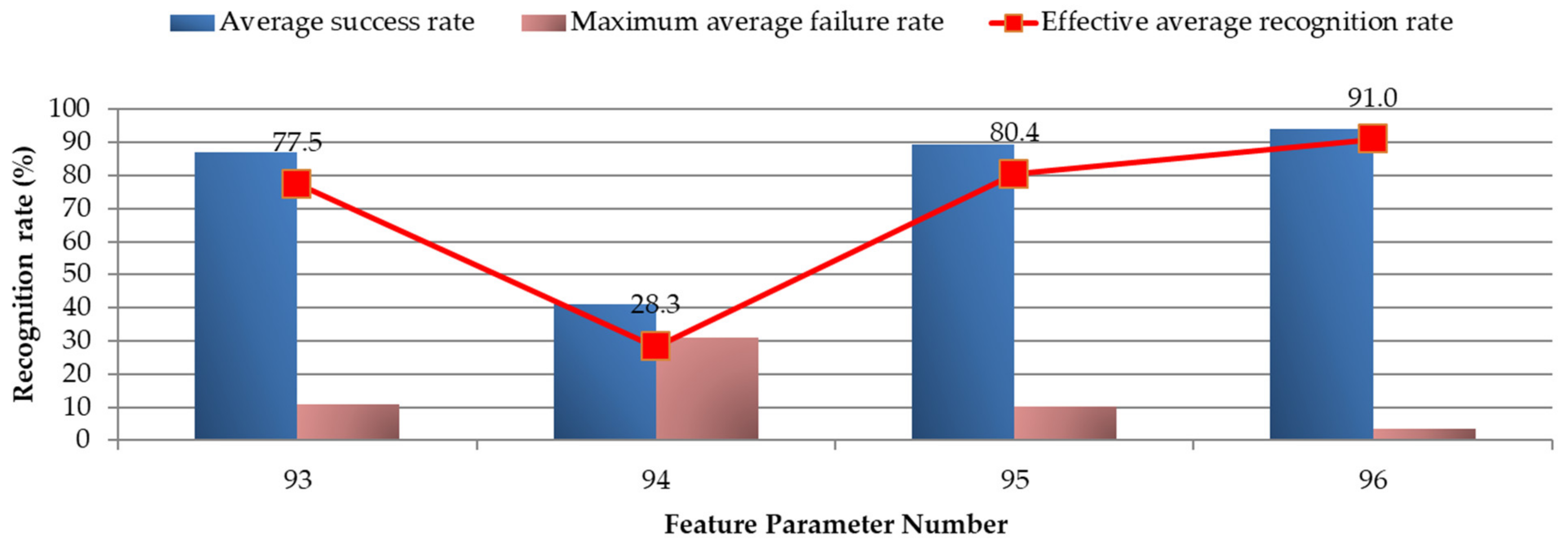
Table 9.
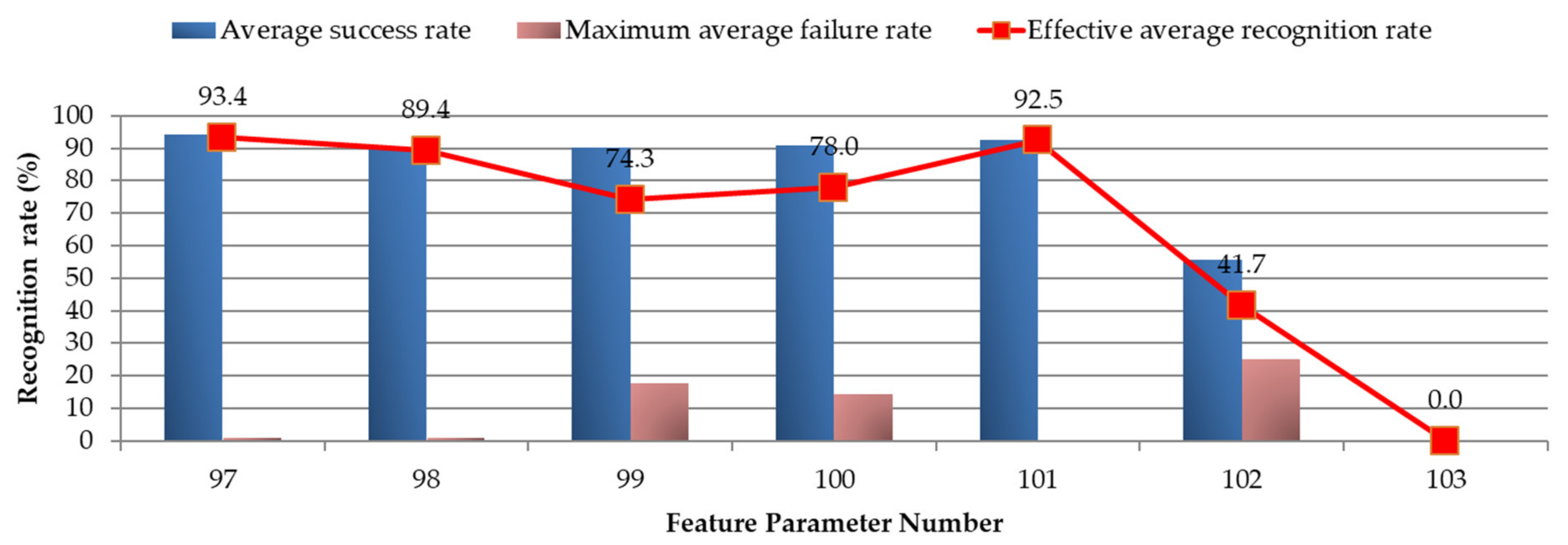
GIS-1 best recognition rate of characteristic parameters: discharge intensity distribution.
Table 9.
GIS-1 best recognition rate of characteristic parameters: discharge intensity distribution.
| Feature Parameters | RECAS | RECF | RECEA |
|---|
| No. | Name | Average Success Rate | Maximum Average Failure Rate | Effective Average Recognition Rate |
|---|
| 97 | Average value of discharge intensity | 94.2 | 0.9 | 93.4 |
Table 10.
GIS-2 better recognition rate: basic discharge parameters.
Table 10.
GIS-2 better recognition rate: basic discharge parameters.
| Feature Parameters | RECAS | RECF | RECEA |
|---|
| No. | Name | Average Success Rate | Maximum Average Failure Rate | Effective Average Recognition Rate |
|---|
| 1 | Total discharge of the whole cycle | 97.5 | 0 | 97.5 |
Table 11.
GIS-2 best recognition rate of the characteristic parametric: cross-correlation coefficients.
Table 11.
GIS-2 best recognition rate of the characteristic parametric: cross-correlation coefficients.
| Feature Parameters | RECAS | RECF | RECEA |
|---|
| No. | Name | Average Success Rate | Maximum Average Failure Rate | Effective Average Recognition Rate |
|---|
| 95 | Average discharge volume and phase correlation coefficient of positive and negative half-cycle | 96.6 | 2.5 | 94.2 |
Table 12.
GIS-2 better recognition rate of the characteristic parameters: discharge intensity distribution.
Table 12.
GIS-2 better recognition rate of the characteristic parameters: discharge intensity distribution.
| Feature Parameters | RECAS | RECF | RECEA |
|---|
| No. | Name | Average Success Rate | Maximum Average Failure Rate | Effective Average Recognition Rate |
|---|
| 97 | Average value of discharge intensity | 97.4 | 1.7 | 95.8 |
Table 13.
GIS-3 best recognition rate: basic discharge parameters.
Table 13.
GIS-3 best recognition rate: basic discharge parameters.
| Feature Parameters | RECAS | RECF | RECEA |
|---|
| No. | Name | Average Success Rate | Maximum Average Failure Rate | Effective Average Recognition Rate |
|---|
| 2 | Number of discharges in the whole cycle | 100 | 0 | 100 |
Table 14.
GIS-3 best recognition rate of the characteristic parameters: cross-correlation coefficients.
Table 14.
GIS-3 best recognition rate of the characteristic parameters: cross-correlation coefficients.
| Feature Parameters | RECAS | RECF | RECEA |
|---|
| No. | Name | Average Success Rate | Maximum Average Failure Rate | Effective Average Recognition Rate |
|---|
| 93 | Correlation coefficient of sum-phase of positive and negative half-cycle discharges | 93.3 | 0.0 | 93.3 |
Table 15.
GIS-3 better recognition rate of the characteristic parameters: discharge intensity distribution.
Table 15.
GIS-3 better recognition rate of the characteristic parameters: discharge intensity distribution.
| Feature Parameters | RECAS | RECF | RECEA |
|---|
| No. | Name | Average Success Rate | Maximum Average Failure Rate | Effective Average Recognition Rate |
|---|
| 98 | Standard deviation of discharge intensity | 99.1 | 0.0 | 99.1 |
Table 16.
Parallel recognition system feature numbers.
Table 16.
Parallel recognition system feature numbers.
| | Group | I | II | III |
|---|
| Description | |
|---|
| ANFIS-1 | 1 | 96 | 97 |
| ANFIS-2 | 1 | 95 | 97 |
| ANFIS-3 | 2 | 93 | 98 |


