Energy Efficiency of Pressure Shock Damper in the Hydraulic Lifting and Leveling Module

Abstract

This study evaluates the energy efficiency of pressure shock damping in a hydraulic lifting and leveling (HLL) module of a mobile robotic bricklaying system (RBS). The HLL module includes a servohydraulic actuator (SHA) and a hydraulic shock damper (HSD). The proposed adjustable HSD consists of a hydraulic accumulator circuit (HAC) and proportional damping valve. The frequency characteristics of the impedance and damping efficiency indices were used to evaluate the effectiveness of HSD damping. The dynamic responses of the SHA with and without HSD were analyzed based on a nonlinear state-space model. To control the damping of the pressure shock in the SHA-HSD system, a linear quadratic Gaussian (LQG) controller that follows two measurement signals was implemented. The LQG controller was adapted to the specific dynamic requirements of the SHA-HSD control system and nature of the RBS shock loads. The effectiveness of the LQG controller was evaluated during RBS operation under laboratory conditions. The main purpose of this study was to dynamically stabilize a leveled robot base subjected to shock loading during automatic operation of the RBS.

1. Introduction

The dynamic properties and precision of the hydraulic servo drive control depend on the dynamic loads, vibrations, and the rigidity mounting of the hydraulic elements [1]. Vibrations of hydraulic elements are noticeable, particularly in vehicles on rough roads, heavy vehicles, aircraft, construction equipment, road vehicles, road-making machines, heavy-duty machines, agricultural machinery, mining machinery, steel industry machines, lifting equipment, transportation equipment, heavy manipulators, and robots. Vibrations of the mechanical elements are transmitted to pulsations of the flow in the hydraulic systems. The operation of heavy hydraulic machines with changing load mass and external shock forces causes the formation of vibrations and deformation of structural elements and the connecting devices of hydraulic systems. The dynamic properties of the hydraulic drive change dramatically when the hydraulic actuators are loaded with shock force. This situation often occurs in hydraulic suspension machines and vehicles such as rolling mills, tracked vehicles, and wheeled vehicles [2]. For safety reasons, hydraulic components should be mounted in a manner that is resistant to excitation vibrations [3]. Military standards (MIL-STD) also require compliance with good practices in the field of operation of vibrating loaded hydraulic systems [4]. Vibrations and shock forces affect technical devices and machines, leading to failure or damage to structural elements. Excess vibrations are a common problem during the operation of hydraulic drives. In the design hydraulic servo drives, the natural vibrations of the hydraulic elements and external mechanical excitations are generally not considered. Due to the safe operation of hydraulic systems, they must be protected against the influence of external vibrations [5]. Physical damage to hydraulic actuators is typically caused by external vibrations induced by unevenly distributed payloads. Damage to the actuator may be in the form of a bent piston rod or a dented barrel, which prevents the full stroke of the piston. A hydraulic cylinder can be a single point of failure, meaning that its reliability is crucial in hydraulic drive systems [6]. Robots for heavy loads and wide operating space have become popular research objects for control engineers due to their sophisticated dynamic properties [7]. The approach to active damping control for multilink robots uses a spring damping element, which is a passive energy dissipation device [8].

As this study concerns HSD in the HLL module of the mobile RBS, commercially available masonry robots were reviewed. With the move to Industry 4.0, robots are starting to appear within the construction industry landscape. With the labor shortages experienced in all countries, innovators are turning to robotics to help plug the gap in skilled trade. One of the most well-known construction robots is the Hadrian X bricklaying robot, developed by FBR in Australia, which is mounted on the boom of a truck crane [9]. The work of this robot is limited to laying masonry blocks from the outside. World reports on construction robots, particularly masonry (bricklaying) robots, are available only on websites in the form of general information about their applications. There is no explicit information on the methodology or research results of masonry robots. The implementation of advanced technology in construction using robots significantly accelerates and leads to an improvement in the quality of bricklaying and plastering work. Recently, productivity improvement has not been a major problem in the construction sector, but there is a lack of a sufficient supply of skilled construction workers. Currently, the construction sector is approaching a decisive period of rapid automation and robotization of traditional and innovative technological processes. Robotics is considered a potential solution for improving the efficiency of the construction industry. There have been many reports in literature on the implementation of masonry robots. A study [10] presented research on the possibility of automating masonry; a masonry robot capable of autonomously building walls using cinder blocks was designed. Pritschow et al. demonstrated an automated masonry construction process on a building site using a mobile robot [11]. Madsen analyzed the benefits and weaknesses of Semi Automated Mason (SAM100) cooperating with a mason worker, which smooths out excess mortar [12]. SAM100 is more effective for large box-shaped structures, such as warehouses. These structures are primarily composed of bricks and other masonry materials. An alternative method is panelization or prefabrication of brick panels in a plant environment [13]. Scientific and applied research evaluating the potential use of robots in construction is essential.

2. Hydraulic Lifting and Leveling Module

2.1. RBS Project

The authors of this study, as researchers in cooperation with the industrial partner Strabag Ltd. Poland, conducted an innovative research project aimed at designing, manufacturing, and implementing the first mobile RBS in Poland. Strabag is a large international company that focuses on building, construction, civil engineering, and transportation infrastructures. Figure 1 shows a 3D model of the mobile RBS.

This RBS project was designed for masonry technology classified as “mobile masonry robot”. The main applications of mobile RBS are the facades and partition walls of offices and residential buildings, as well as industrial halls. Mobile RBS enables bricklaying of walls with dimensions limited to the working space of the robot. RBS optimized the time, cost, and efficiency of masonry work and reduced the amount of waste. The mobile RBS is characterized by a new and innovative design solution, the task of which is to robotize the time-consuming and heavy bricklaying work traditionally performed by hand by masons.

The bricklaying robot picks up the bricks, puts the mortar on them, and places the bricks on the wall. The robotic bricklaying process is shown in Figure 2.

The RBS consists of a six degrees-of-freedom (6-DoF) ABB bricklaying robot (IRB 4600) with a replaceable hydraulic gripper, a Hinowa tracked undercarriage with a hydraulic unit, an RBS, an HLL module, a brick warehouse, a brick feeder, a mortar applicator, a control cabinet, and a control panel. Before starting work, the mobile RBS travels to the bricklaying site and is then lifted, leveled, and anchored. Bricklaying begins with the precise positioning of the robot according to the wall plan using laser sensors. The bricklaying robot has a weight of 450 kg, a gripper load of 40 kg, a maximum vertical range of 3.055 m, and a maximum horizontal range of 2.55 m.

2.2. HLL Module Operation

In previous studies, the authors analyzed the electrohydraulic control and kinematic model of the HLL module of an RBS [14,15,16]. The main task of the HLL module is to lift the RBS to the desired height and precisely level it. Leveling of an RBS occurs in two stages: maximum extension of the supporting legs by means of a short-stroke actuators, and then lifting and leveling by means of a lifting actuators. In the first stage, the actuators extend the supporting legs without external load until they come into contact with the ground. In the second stage, the lifting actuators press the supporting legs until the tracked platform is raised to the required height. This is followed by the servohydraulic leveling process in which the hydraulic actuators level the RBS at a specific height. Once leveled, the RBS is mechanically locked. RBS hydraulic lifting and leveling is justified in cases where:

• Fast and precise levelling is required under heavy loads;
• Lifting and leveling are frequent;
• The lifting and leveling system must be durable and solid.

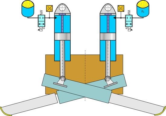
Two HLL modules were used to lift and level the RBS, which also stabilizes the position of the RBS during automatic bricklaying. A single HLL module was constructed of two hydraulically lifting support legs mounted in a cross system. The view of the HLL module with an extendable supporting leg and the cross system of the hydraulic lifting actuators for the supporting legs is shown in Figure 3.

Automatic operation of a heavy bricklaying robot consisting of placing bricks of different weights in a large workspace causes variable dynamic shock loads on the RBS. The shock loads of the RBS are transmitted to the mechanical construction joints and hydraulic elements of the HLL module. High shock loads cause excessive vibration and damage to mechanical and hydraulic components, as well as incorrect control of the trajectories of the bricklaying robot. As a result of shock loading of the RBS, pressure pulsation and pressure shock wave (water hammer) are generated in the hydraulic actuators of the HLL modules, then damage the hydraulic components, increase the noise level and affect deterioration of the quality of the servohydraulic system; thus not leveling the RBS. The pulse or shock pressure in hydraulic actuators can manifest itself when the robot arm is „buckling”. To prevent these unfavorable phenomena in hydraulic systems, hydraulic shock absorbers are used. After testing the automatic bricklaying at different shock loads of the robot and mobile platform, it was decided to equip the HLL module with an HSD.

2.3. SHA-HSD System

Due to the constantly changing external SHA shock load, the use of an adjustable HSD is warranted. The use of an HSD reduces the effects of pressure shock in the SHA (actuator, valve, and pipeline) of the HLL module. The subject of research is the effectiveness of adjustable HSD in the SHA-HSD system in a HLL of an RBS. A schematic diagram of an SHA-HSD system is shown in Figure 4.

The SHA consists of a hydraulic lift actuator (double-acting with one-sided piston rod) with an internal magnetostrictive linear position transducer, a 4WRE proportional directional valve, directly operated with position feedback and integrated control electronics (ICEs). The parameters of a hydraulic lift actuator are the diameter of the piston D = 0.05 m, the diameter of the piston rod d = 0.028 m, area ratio α = 0.69, stroke h = 1.25 m, and working pressure p = 25 MPa. Technical data of the 4/3 proportional directional valve: nominal volumetric flow rate q_vn = 35 L/min (0.583 × 10⁻³ m³s⁻¹) at a pressure difference of Δp_n = 1 MPa. An adjustable HSD consists of a 2-way proportional throttling valve, where a damping valve dissipates shock energy, a hydropneumatic accumulator absorb pressure shock, and a pressure transducer. The proportional throttle valve consists of the main valve with a nominal N25 orifice and the pilot control valve with a proportional solenoid. The flow through the valve depends on the pressure drop Δp across the orifice and the position of the orifice spool z, and the command value u = 0–10 V. The maximum operating pressure of the valve was 31.5 MPa and the maximum flow rate of the operating fluid was 38 L/min (0.63 × 10⁻³ m³s⁻¹). The flow resistance of the damping valve is adjusted by the voltage of the proportional solenoid coil. The shift of the valve spool is proportional to the coil voltage, increasing or decreasing the flow resistance. In an applied diaphragm accumulator with a nominal volume of 1 L (0.001 m³) and permission pressure ratio 10:1, a flexible diaphragm separates the compressible gas cushion from the working hydraulic fluid. Hydropneumatic accumulators are based on the principle of using nitrogen as a compressible medium. When a proportional damping valve is placed between the hydraulic actuator and the accumulator, an adjustable damping is achieved, which occurs in semiactive shock absorbers. Hydraulic accumulators up to a nominal volume of 2 L can be screwed directly into the connecting tube. An HSD can be fabricated in size and form suitable for installation near the SHA or a master actuator.

The main purpose of this work was to stabilize a leveled RBS subjected to shock loading during the automatic operation of the RBS. The goal was achieved by:

• Design, simulation, and practical testing of an SHA-HSD system;
• Simulation tests to determine the frequency characteristics and dynamic responses of an SHA-HSD system;
• Implementation of the linear quadratic Gaussian (LQG) controller to the specific dynamic requirements of the SHA-HSD control system and an RBS load;
• Design of the LQG controller that follows two measurement signals;
• Evaluation of the effectiveness of the LQG controller during RBS operation under laboratory conditions.

In particular, the objective of the study was to provide a shock pressure damper in the form of an HSD solution that responds rapidly, dampens the increase in pressure, and dissipates the energy of the input shock forces in the SHA.

3. HSD Frequency Analysis

3.1. Transfer Function of the HAC

The hydropneumatic accumulator with a connecting pipeline between the accumulator and valve, called the hydraulic accumulator circuit (HAC), can be modeled by a lumped circuit containing elements of resistance R_h, inductance L_h, and capacitance C_h [17].

$${{\displaystyle L}}_h\hspace{0.17em}\frac{{{\displaystyle dq}}_c}{dt}+{{\displaystyle R}}_h\hspace{0.17em}{{\displaystyle q}}_c={{\displaystyle p}}_c-{{\displaystyle p}}_a$$

(1)

$${{\displaystyle q}}_c={{\displaystyle C}}_a\hspace{0.17em}\frac{{{\displaystyle dp}}_a}{dt}\hspace{0.17em}\Rightarrow \hspace{0.17em}\frac{{{\displaystyle dp}}_a}{dt}=\frac{1}{{{\displaystyle C}}_a}{{\displaystyle q}}_c$$

(2)

where q_c is the flow rate in the connecting tube, p_a is the pressure of the gas (nitrogen) in the accumulator, p_c is the pressure in the connecting tube, and L_h is the hydraulic inductance of the connecting tube,

$${{\displaystyle L}}_h\hspace{0.17em}\hspace{0.17em}=\frac{\rho \hspace{0.17em}a}{{{\displaystyle \pi \hspace{0.17em}r}}^2}$$

(3)

where r is the inner radius of the connecting tube (r = 0.0025 m), ρ is the density of ISO 32 hydraulic mineral oil (ρ = 866 kg/m³ at 16 °C), and a is the velocity of the sound

$$a\hspace{0.17em}=\sqrt{\frac{K}{\rho }}$$

(4)

where K is the bulk modulus of ISO 32 mineral oil (K = 1800 MPa), and R_h is the hydraulic resistance of the connecting pipe determined from the Hagen-Poiseuille equation;

$${{\displaystyle R}}_h\hspace{0.17em}=\frac{8\hspace{0.17em}l\hspace{0.17em}\nu \hspace{0.17em}\rho }{\pi {{\displaystyle \hspace{0.17em}r}}^4}$$

(5)

where l is the length of the connecting pipeline (l = 0.01 m), ν is the kinematic viscosity of ISO 32 mineral oil (ν = 32 × 10⁻⁶ m²/s at 40 °C), and C_a is the gas capacitance of the hydropneumatic accumulator,

$${{\displaystyle C}}_a=\frac{dV}{dp}=\frac{{{\displaystyle V}}_0}{n\hspace{0.17em}{{\displaystyle p}}_0}{{\displaystyle \left(1-\frac{\Delta V}{{{\displaystyle V}}_0}\right)}}^{\kappa +1}\approx \frac{{{\displaystyle V}}_0}{\kappa \hspace{0.17em}{{\displaystyle p}}_0}$$

(6)

where p₀ is the initial pressure (p₀ = 10 MPa), V₀ is the initial volume (V₀ = 0.001 m³), and κ is the adiabatic exponent in case of nitrogen (κ = 1.4).

The compression and expansion processes taking place in hydropneumatic accumulators are governed by the general gas laws. For pressures up to 20 MPa, the real behavior of nitrogen does not differ from the adiabatic process of an ideal gas.

By the differentiation of Equation (1) and substituting Equation (2), it is obtained;

$${{\displaystyle C}}_a\hspace{0.17em}{{\displaystyle L}}_h\hspace{0.17em}\hspace{0.17em}\frac{{{\displaystyle d}}^2{{\displaystyle q}}_c}{{{\displaystyle dt}}^2}+{{\displaystyle C}}_a\hspace{0.17em}{{\displaystyle R}}_h\hspace{0.17em}\frac{{{\displaystyle dq}}_c}{dt}+{{\displaystyle q}}_c={{\displaystyle C}}_a\frac{{{\displaystyle dp}}_c}{dt}$$

(7)

After applying the Laplace transform, Equation (7) takes the form of a transfer function:

$${{\displaystyle G}}_a(s)=\frac{{{\displaystyle q}}_c(s)}{{{\displaystyle p}}_c(s)}=\frac{{{\displaystyle C}}_a\hspace{0.17em}s}{{{\displaystyle C}}_a\hspace{0.17em}{{\displaystyle L}}_h\hspace{0.17em}{{\displaystyle s}}^2+{{\displaystyle C}}_a\hspace{0.17em}{{\displaystyle R}}_h\hspace{0.17em}s+1}=\frac{{{\displaystyle C}}_a\hspace{0.17em}s}{\frac{1}{{{\displaystyle \omega }}_n^2}\hspace{0.17em}{{\displaystyle s}}^2+\frac{2\hspace{0.17em}\zeta }{\hspace{0.17em}{{\displaystyle \omega }}_n}\hspace{0.17em}s+1}$$

(8)

where ω_n is the natural frequency.

$${{\displaystyle \omega }}_n=\frac{1}{\sqrt{{{\displaystyle C}}_a\hspace{0.17em}{{\displaystyle L}}_h}}$$

(9)

ζ is the damping ratio,

$$\zeta =\frac{1}{2\hspace{0.17em}}\hspace{0.17em}{{\displaystyle C}}_a\hspace{0.17em}{{\displaystyle R}}_h\hspace{0.17em}{{\displaystyle \omega }}_n$$

(10)

The transfer function (8) in the frequency domain has the form:

$${{\displaystyle G}}_a(j\omega )=\frac{{{\displaystyle q}}_c(j\omega )}{{{\displaystyle p}}_c(j\omega )}=\frac{{{\displaystyle C}}_a\hspace{0.17em}j\hspace{0.17em}\omega }{1-\frac{{{\displaystyle \omega }}^2}{{{\displaystyle {{\displaystyle \omega }}_n}}^2}+\hspace{0.17em}\frac{2\hspace{0.17em}\zeta }{\hspace{0.17em}{{\displaystyle \omega }}_n}\hspace{0.17em}j\omega }=\frac{1}{\alpha \hspace{0.17em}\left[\beta +j\left(\frac{\omega }{{{\displaystyle \omega }}_n}-\frac{{{\displaystyle \omega }}_n}{\omega }\right)\right]}$$

(11)

where α and β are the constant coefficients.

$$\alpha =\frac{1}{{{\displaystyle C}}_a\hspace{0.17em}{{\displaystyle \omega }}_n}$$

(12)

$$\beta =2\hspace{0.17em}\zeta$$

(13)

3.2. Impedance of the HAC

Pressure waves in a hydraulic line can be modeled in the frequency domain using the impedance Z(jω), which, analogously to the electrical impedance in alternating current circuits (voltage-current ratio), is determined by the ratio of pressure p_c and flow rate q_c:

$$Z(j\omega )=\frac{{{\displaystyle p}}_c(j\omega )}{{{\displaystyle q}}_c(j\omega )}\hspace{0.17em}\hspace{0.17em}\hspace{0.17em}\hspace{0.17em}\mathrm{in}\hspace{0.17em}\hspace{0.17em}\frac{\mathrm{N}\hspace{0.17em}\mathrm{s}}{{{\displaystyle \mathrm{m}}}^5}$$

(14)

Hydraulic impedance (also known as characteristic impedance) refers to the resistance of the pressure wave inside a hydraulic line.

The impedance Z_a(jω) of the HAC is the reciprocal of (11):

$${{\displaystyle Z}}_a(j\omega )=\frac{{{\displaystyle p}}_c(j\omega )}{{{\displaystyle q}}_c(j\omega )}=\alpha \left[\beta +j\left(\frac{\omega }{{{\displaystyle \omega }}_n}-\frac{{{\displaystyle \omega }}_n}{\omega }\right)\right]$$

(15)

From Equation (15) results the HAC impedance modulus:

$$\left|{{\displaystyle Z}}_a(j\omega )\right|=\alpha \hspace{0.17em}\sqrt{{{\displaystyle \beta }}^2+{{\displaystyle \left(\frac{\omega }{{{\displaystyle \omega }}_n}-\frac{{{\displaystyle \omega }}_n}{\omega }\right)}}^2}$$

(16)

and the HAC impedance argument:

$$\arg \left[{{\displaystyle Z}}_a(j\omega )\right]=\arctan \frac{\left(\frac{\omega }{{{\displaystyle \omega }}_n}-\frac{{{\displaystyle \omega }}_n}{\omega }\right)}{\beta }$$

(17)

Equation (16) was converted to a dimensionless form:

$$\left|{{\displaystyle Z}}_A(j\omega )\right|=\log \left(\frac{\left|{{\displaystyle Z}}_a(j\omega )\right|}{\alpha }\right)=\log \left(\sqrt{{{\displaystyle \beta }}^2+{{\displaystyle \left(\frac{\omega }{{{\displaystyle \omega }}_n}-\frac{{{\displaystyle \omega }}_n}{\omega }\right)}}^2}\right)$$

(18)

The characteristics of the impedance amplitude and impedance phase of the HAC are shown in Figure 5 and Figure 6.

The dimensionless impedance characteristics shown in Figure 5 and Figure 6 are used to select HAC parameters. The purpose of this analysis is to select a parameter that provides a lower HAC impedance. How the HRC parameters influence its natural frequency ω_n is shown in the Equation (9).

3.3. Impedance of the Damping Valve

The best mathematical way to write the impedance of the damping valve is a complex form Z = R + j X, the real part of which is the resistance R of the valve, and the imaginary part is the reactance X of the valve.

The valve reactance is in the form of an inductive reactance X_L = jωL, then

$$Z(j\omega )=R+j\omega \hspace{0.17em}L$$

(19)

or a capacitive reactance X_C = 1/jωC, then

$$Z(j\omega )=R-j\frac{1}{\omega \hspace{0.17em}C}$$

(20)

where ω is the angular frequency, L is the inductance, and C is the capacitance.

The phenomenon of flow through the damping valve can be described not only by the resistance R but also by the inductive effect L observed as a result of the high flow velocity. However, the capacitive effect C can be explained by the compressibility of the volume of fluid contained in the valve chamber between the connection port and the orifice.

The flow rate q_v through the adjustable damping valve has the form;

$${{\displaystyle q}}_{\mathrm{v}}=\hspace{0.17em}{{\displaystyle K}}_q\hspace{0.17em}z\hspace{0.17em}\sqrt{\Delta p}$$

(21)

where Δp is the pressure drop across the valve, and K_q is the valve flow coefficient;

$${{\displaystyle K}}_q\hspace{0.17em}=\frac{{{\displaystyle q}}_{\mathrm{v}n}}{{{\displaystyle z}}_n\hspace{0.17em}\sqrt{{{\displaystyle \Delta p}}_n}}$$

(22)

where q_vn is the nominal flow rate at a pressure drop Δp_n = 1 MPa and z_n is the nominal shift of the valve spool, and z is the shift of a spool valve,

$$z=\frac{{{\displaystyle z}}_{\max }}{{{\displaystyle u}}_{\max }}\hspace{0.17em}u={{\displaystyle K}}_z\hspace{0.17em}u$$

(23)

where u is the input voltage to adjust the damping valve; K_z is the gain factor, z_max is the maximum. deflection of the spool from the center position, $z_{\max }=\max \left(\left|z_{s\min }\right|,\left|z_{s\max }\right|\right)$, z_smin is the minimum spool stroke, and z_smax is the maximum spool stroke, the spool path is limited to z_smin ≤ z ≤ z_smax.

Equation (21) was linearized for small pressure perturbations that provided;

$${{\displaystyle q}}_{\mathrm{v}}={{\displaystyle K}}_q\hspace{0.17em}{{\displaystyle K}}_z\hspace{0.17em}u\hspace{0.17em}\sqrt{\Delta p}\approx \hspace{0.17em}\frac{{{\displaystyle K}}_q\hspace{0.17em}{{\displaystyle K}}_z}{2\hspace{0.17em}\sqrt{{{\displaystyle \Delta p}}_n}}\hspace{0.17em}u\hspace{0.17em}\Delta p=\frac{1}{R}\hspace{0.17em}\hspace{0.17em}\Delta p$$

(24)

where R is the flow resistance of the damping valve,

$$R(u)=\frac{2\hspace{0.17em}\sqrt{{{\displaystyle \Delta p}}_n}}{{{\displaystyle K}}_q\hspace{0.17em}{{\displaystyle K}}_z}\hspace{0.17em}\frac{1}{u}$$

(25)

The dynamic valve model is presented as the first-order differential equation provided by

$$C\hspace{0.17em}\frac{d\Delta p}{dt}+\frac{1}{R}\Delta p={{\displaystyle q}}_{\mathrm{v}}$$

(26)

where C is the capacitance of the valve.

The transform Equation (26) shows the impedance of the damping valve in the form of the PT1 transfer function.

In the Laplace domain:

$${{\displaystyle Z}}_{\mathrm{v}}(s)=\frac{\Delta p(s)}{{{\displaystyle q}}_{\mathrm{v}}(s)}=\frac{R}{1+R\hspace{0.17em}C\hspace{0.17em}s}=\frac{R}{1+T\hspace{0.17em}s}$$

(27)

In the frequency domain:

$${{\displaystyle Z}}_{\mathrm{v}}(j\omega )=\frac{\Delta p(j\omega )}{{{\displaystyle q}}_{\mathrm{v}}(j\omega )}=\frac{R}{1+j\omega \hspace{0.17em}T}$$

(28)

where T is the constant time $T=RC$.

From the impedance of the damping valve, it is possible to remove the capacitive component C by shifting the measurement point where the effective volume is zero. In this case, the impedance of the valve is closer to the simple resistance model, so Equation (28) has the form;

$${{\displaystyle Z}}_{\mathrm{v}}(j\omega )=\frac{\Delta p(j\omega )}{{{\displaystyle q}}_{\mathrm{v}}(j\omega )}=R$$

(29)

3.4. Effectiveness of HSD Damping

The function impedance of the HSD results from the flow continuity equation;

$${{\displaystyle q}}_c=\frac{1}{{{\displaystyle Z}}_a}{{\displaystyle p}}_c={{\displaystyle q}}_{\mathrm{v}}=\frac{1}{{{\displaystyle Z}}_{\mathrm{v}}}\hspace{0.17em}\Delta p=\frac{1}{{{\displaystyle Z}}_{\mathrm{v}}}\hspace{0.17em}\left({{\displaystyle p}}_A-{{\displaystyle p}}_c\right)$$

(30)

substituting q_c = p_c/Z_a provides;

$$\hspace{0.17em}{{\displaystyle p}}_A=\left(1+\frac{{{\displaystyle Z}}_{\mathrm{v}}}{{{\displaystyle Z}}_a}\right){{\displaystyle p}}_c \Rightarrow {{\displaystyle Z}}_p=\frac{{{\displaystyle p}}_A}{{{\displaystyle p}}_c}=1+\frac{{{\displaystyle Z}}_{\mathrm{v}}}{{{\displaystyle Z}}_a}$$

(31)

where p_A is the upstream pressure of the valve in the actuator chamber and p_c is the downstream pressure of the valve in the accumulator.

The impedance function of the HSD was determined from Equation (29) after substituting Equations (15) and (29);

$${{\displaystyle Z}}_p(j\omega )=\frac{{{\displaystyle p}}_A}{{{\displaystyle p}}_c}=1+\frac{{{\displaystyle Z}}_{\mathrm{v}}(j\omega )}{{{\displaystyle Z}}_a(j\omega )}=1+\frac{R}{\alpha \beta +\alpha j\left(\frac{\omega }{{{\displaystyle \omega }}_n}-\frac{{{\displaystyle \omega }}_n}{\omega }\right)}$$

(32)

The modulus of the impedance function was determined as follows;

$$\left|{{\displaystyle Z}}_p(j\omega )\right|=\sqrt{1+\frac{{{\displaystyle R}}^2+2R\hspace{0.17em}\alpha \beta }{{{\displaystyle \alpha }}^2{{\displaystyle \beta }}^2+{{\displaystyle \alpha }}^2{{\displaystyle \left(\frac{\omega }{{{\displaystyle \omega }}_n}-\frac{{{\displaystyle \omega }}_n}{\omega }\right)}}^2}}$$

(33)

The effectiveness of shock pressure damping as a function of frequency depending on various parameters was evaluated using the following damping efficiency index as a quality index;

$$D(\omega )=20\hspace{0.17em}\log \left|{{\displaystyle Z}}_p(j\omega )\right|\hspace{0.17em}\hspace{0.17em}\hspace{0.17em}dB$$

(34)

Figure 7 shows the damping efficiency index as a function of the frequency ratio for different input voltages u of the damping valve at the upstream pressure p_A = 1 MPa.

Figure 8 shows the damping efficiency index as a function of the frequency ratio for different upstream pressures p_A at the input voltage u = 5 V of the damping valve.

When determining the damping efficiency index D, the resistance R as a function of the voltage u was taken into account in accordance with Equation (25). The lower the voltage u on the valve coil, the smaller the z shift of the valve spool; therefore, the higher the flow resistance R. Then the damping efficiency is higher. Damping efficiency indices as a function of the frequency ratio shown in Figure 7 and Figure 8 are used to select the parameters p_A and u of the SHA-HSD system due to the effectiveness of pressure shock damping.

4. Dynamic Responses of the SHA-HSD System

According to Equations (1), (2) and (30), the dynamic model of the HSD was saved in the time domain;

$$\{\begin{array}{l}{{\displaystyle \dot{q}}}_c=\frac{1}{{{\displaystyle L}}_h}\left[-\left({{\displaystyle R}}_h+R\right)\hspace{0.17em}{{\displaystyle q}}_c+{{\displaystyle p}}_A-{{\displaystyle p}}_a\right]\\ {{\displaystyle \dot{p}}}_a=\frac{1}{{{\displaystyle C}}_a}{{\displaystyle q}}_c\end{array}$$

(35)

For a set lift and level of the RBS, the dynamic model of an SHA excited by the shock load is as follows;

$$\{\begin{array}{l}\ddot{y}=\frac{1}{m}\left[-b\hspace{0.17em}\dot{y}-\left({{\displaystyle A}}_A\hspace{0.17em}{{\displaystyle p}}_A-{{\displaystyle A}}_B\hspace{0.17em}{{\displaystyle p}}_B\right)+W+F(t)\right]\\ {{\displaystyle \dot{p}}}_A=\frac{1}{{{\displaystyle C}}_A}\hspace{0.17em}\left(-{{\displaystyle q}}_c+{{\displaystyle A}}_A\hspace{0.17em}\dot{y}\right)\\ {{\displaystyle \dot{p}}}_B=-\frac{1}{{{\displaystyle C}}_B}\hspace{0.17em}{{\displaystyle A}}_B\hspace{0.17em}\dot{y}\end{array}$$

(36)

where y is the displacement of the valve piston, m is the mass load, b is the damping coefficient of the hydraulic actuator, W is the weight load of the lifting actuators, F(t) is the time-varying shock force acting on the lifting actuators, and C_A and C_B are the hydraulic capacitances of the actuator chambers

$${{\displaystyle C}}_A=\frac{{{\displaystyle V}}_A}{K}$$

(37)

$${{\displaystyle C}}_B=\frac{{{\displaystyle V}}_B}{K}$$

(38)

where K is the bulk oil modulus, and V_A and V_B are the volume of the actuator chambers;

$${{\displaystyle V}}_A={{\displaystyle V}}_{A0}+{{\displaystyle A}}_A\hspace{0.17em}{{\displaystyle y}}_s$$

(39)

$${{\displaystyle V}}_B={{\displaystyle V}}_{B0}+{{\displaystyle A}}_B\hspace{0.17em}\left(h-{{\displaystyle y}}_s\right)$$

(40)

where V_A0 and V_B0 are the dead volumes of the actuator chamber, A_A and A_B are the effective area of the actuator piston, y_s is the lift position of the actuator piston, and h is the stroke of the actuator piston.

4.1. Determination of the Force Acting on the Lifting Actuators

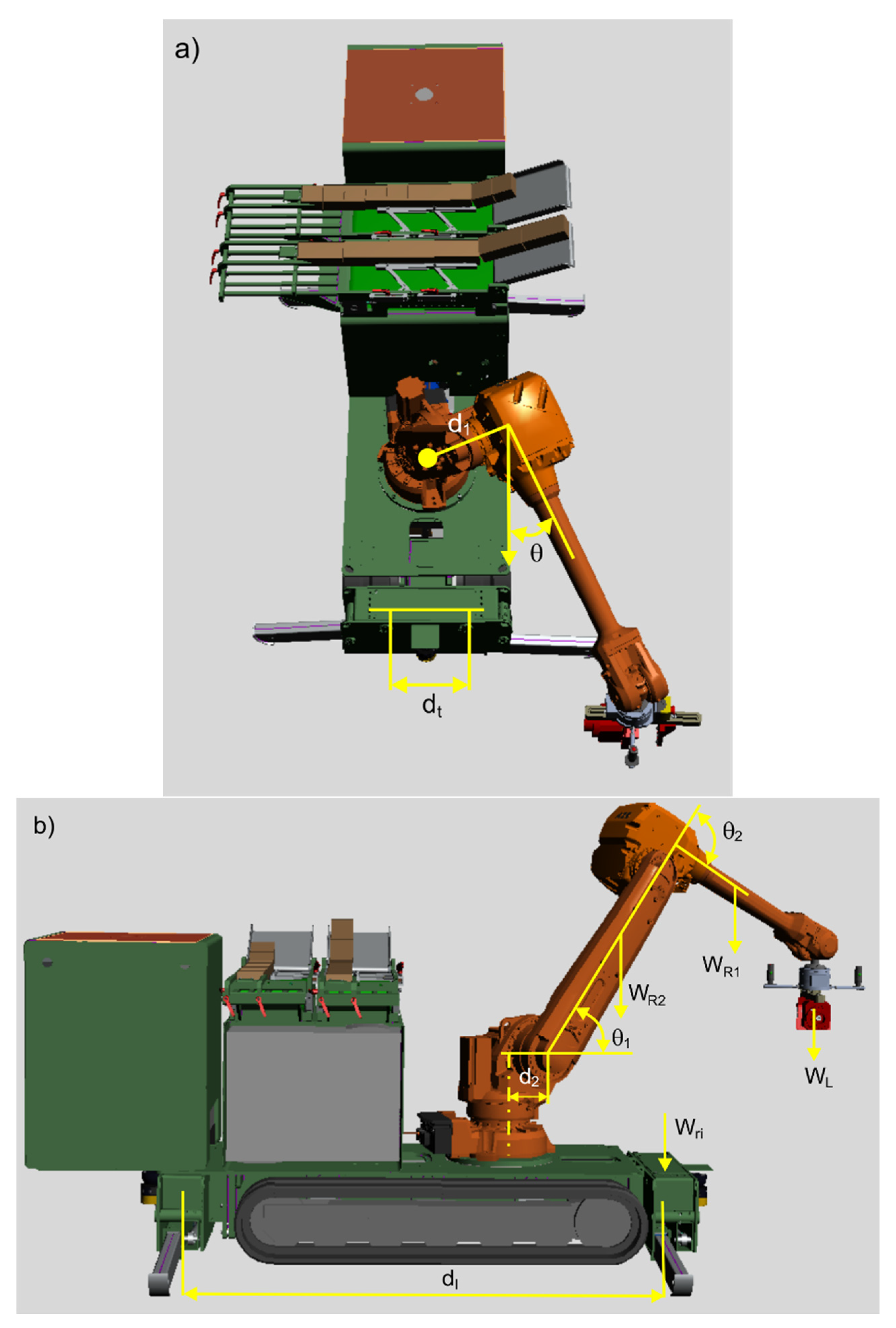
A method was developed to calculate the value of the weight loads of the lifting actuators depending on the angle of movement of the robot arm. The basic parameters for calculating the forces that act on the hydraulic lifting actuators are marked on the RBS, shown in Figure 9.

The value of the weight load of the i-th hydraulic lifting actuators was determined on the basis of the RBS model;

$${{\displaystyle W}}_i=\frac{1}{4}\frac{{{\displaystyle W}}_R+{{\displaystyle W}}_L}{\cos \theta }+{{\displaystyle W}}_{ri}$$

(41)

where W_i is the weight load of the i-th actuator, i = 1,2…4 (1—left front, 2—right front, 3—left rear, and 4—right rear), α is the angle of vertical deviation of the lifting cylinder, W_R is the weight of the two-link robot arm, W_R = W_R1 + W_R2, W_R1 is the weight of the first link of a robot, W_R1 is the weight of the second link of a robot, M_L is the weights of the lifted load (griper, brick), θ is the horizontal swing angles of the robot arm, and W_ri is the vertical reaction;

$$\{\begin{array}{l}{{\displaystyle W}}_{r1}=\frac{1}{2}\hspace{0.17em}\left(\frac{M\hspace{0.17em}\sin \theta }{{{\displaystyle d}}_t}+\frac{M\hspace{0.17em}\cos \theta -\left({{\displaystyle W}}_R+{{\displaystyle W}}_L\right)\hspace{0.17em}a}{{{\displaystyle d}}_l}\right)\\ {{\displaystyle W}}_{r2}=-\frac{1}{2}\hspace{0.17em}\left(\frac{M\hspace{0.17em}\sin \theta }{{{\displaystyle d}}_t}-\frac{M\hspace{0.17em}\cos \theta -\left({{\displaystyle W}}_R+{{\displaystyle W}}_L\right)\hspace{0.17em}a}{{{\displaystyle d}}_l}\right)\\ {{\displaystyle W}}_{r3}=\frac{1}{2}\hspace{0.17em}\left(\frac{M\hspace{0.17em}\sin \theta }{{{\displaystyle d}}_t}-\frac{M\hspace{0.17em}\cos \theta -\left({{\displaystyle W}}_R+{{\displaystyle W}}_L\right)\hspace{0.17em}a}{{{\displaystyle d}}_l}\right)\\ {{\displaystyle W}}_{r4}=-\frac{1}{2}\hspace{0.17em}\left(\frac{M\hspace{0.17em}\sin \theta }{{{\displaystyle d}}_t}+\frac{M\hspace{0.17em}\cos \theta -\left({{\displaystyle W}}_R+{{\displaystyle W}}_L\right)\hspace{0.17em}a}{{{\displaystyle d}}_l}\right)\end{array}$$

(42)

where d_t is the distance between hydraulic actuators in the transverse direction; d_l is the distance between hydraulic actuators in the longitudinal direction, a is the distance between the robot centerline and the center of robot rotation, and M is the moment,

$$M={{\displaystyle W}}_{R1}\hspace{0.17em}{{\displaystyle L}}_{1c}\hspace{0.17em}\cos {{\displaystyle \theta }}_1+{{\displaystyle W}}_{R2}\left({{\displaystyle L}}_1\hspace{0.17em}\cos {{\displaystyle \theta }}_1+{{\displaystyle L}}_{2c}\hspace{0.17em}\cos ({{\displaystyle \theta }}_1-{{\displaystyle \theta }}_2)\right)\hspace{0.17em}$$

(43)

where L₁ is the length of the first link, is the length to the center of gravity of the first link, and L_2c is the length to the center of gravity of the second link, and θ₁ and θ₂ are the vertical swing angles of the robot forearm and arm.

The value of the shock force of the i-th hydraulic lifting actuator was determined from the RP reaction developed during the robot’s motion,

$${{\displaystyle F}}_i(t)=\hspace{0.17em}\frac{1}{4}\frac{{{\displaystyle F}}_q(t)}{\cos \alpha }\hspace{0.17em}$$

(44)

where F_q(t) is the vertical reaction of the supporting actuators.

To determine the value of the force F_q(t), a MATLAB-based Robotics System Toolbox (RST) simulation model was used for the inverse kinematic solution of the six-rotary joint (6-DoF) robot arm. Whatever method is chosen to obtain the dynamic model of the robot arm, it has the following form of a nonlinear equation of force;

$${{\displaystyle F}}_q(t)=\hspace{0.17em}M(q)\hspace{0.17em}\ddot{q}+C(q,\dot{q})+G(q)$$

(45)

where q ∈ Rⁿ is the angular position of a joint, n is the number of joints or the degree of freedom, M(q) ∈ R^nxn is the inertia matrix, C($q$,$\dot{q}$) ∈ R^nxn is a matrix of Coriolis force and centrifugal forces, G(q) is the torque exerted by gravity.

The choice of excitation trajectory is an important consideration when identifying the shock force generated by the robot. For the simulation experiment, a periodic excitation trajectory was selected which takes the form of a finite Fourier series. The angular position q_i for each joint was written as a finite Fourier series. If all elements of the series have the same fundamental frequency ω, then the motion becomes periodic,

$${{\displaystyle q}}_i(t)=\hspace{0.17em}{{\displaystyle q}}_{0i}+{\displaystyle \sum _{k=1}^N{{\displaystyle a}}_k^i\hspace{0.17em}sin(k\omega \hspace{0.17em}t+{{\displaystyle \phi }}_k^i)}\hspace{0.17em}$$

(46)

where a is the Fourier coefficient, φ is the phase shift, k is the number of cycles, and N is theoretically infinite.

The excitation trajectory was implemented in the editor for rapid code iteration. The speed and acceleration of the joints can be obtained by analytically differentiating Equation (46). To simplify the simulation, we assume that all joints are excited simultaneously. The kinematic and dynamic parameters of the robot are limited by the course of the bricklaying process. Therefore, the excitation trajectory was then programmed in ABB Robot-Studio, where a simulation tool was used to visualize the robot’s trajectory during bricklaying (Figure 10).

4.2. Simulation Results

Based on Equations (35) and (36), the simulation model was determined as a nonlinear state-space model (sixth-order differential equation) of the SHA-HSD system. Defining the state variables ${\left[x_{1 }{x}_{2 }{x}_{3 }{x}_{4 }{x}_{5 }{x}_{6 }\right]}^T\widehat{=}{\left[y \dot{y} p_{A }{p}_{B }{q}_c p_a\right]}^T$, the state equation has the form

$$\{\begin{array}{l}{{\displaystyle \dot{x}}}_1={{\displaystyle x}}_2\\ {{\displaystyle \dot{x}}}_2=\frac{1}{m}\left(-b\hspace{0.17em}{{\displaystyle x}}_2-{{\displaystyle A}}_A\hspace{0.17em}{{\displaystyle x}}_3+{{\displaystyle A}}_B\hspace{0.17em}{{\displaystyle x}}_4\right)+\frac{1}{m}\hspace{0.17em}{{\displaystyle F}}_L\\ {{\displaystyle \dot{x}}}_3=\frac{1}{{{\displaystyle C}}_A}\left({{\displaystyle A}}_A\hspace{0.17em}{{\displaystyle x}}_2-{{\displaystyle x}}_5\right)\\ {{\displaystyle \dot{x}}}_4=-\frac{1}{{{\displaystyle C}}_B}\hspace{0.17em}{{\displaystyle A}}_B\hspace{0.17em}{{\displaystyle x}}_2\\ {{\displaystyle \dot{x}}}_5=\frac{1}{{{\displaystyle L}}_h}\left[{{\displaystyle x}}_3-\left({{\displaystyle R}}_h\hspace{0.17em}+R\right){{\displaystyle x}}_5-{{\displaystyle x}}_6\right]\\ {{\displaystyle \dot{x}}}_6=\frac{1}{{{\displaystyle C}}_a}{{\displaystyle x}}_5\hspace{0.17em}\end{array}$$

(47)

where F_L is the external loads, F_L = W_i + F_i.

The state Equation (47) has the matrix form

$$\dot{x}=A\hspace{0.17em}x(t)+B\hspace{0.17em}{F}_L(t)$$

(48)

where A is the state matrix, B is the input matrix,

$$A=\left[\begin{array}{cccccc}0& 1& 0& 0& 0& 0\\ 0& \frac{-b}{m}& \frac{-{{\displaystyle A}}_A}{m}& \frac{{{\displaystyle A}}_B}{m}& 0& 0\\ 0& \frac{{{\displaystyle A}}_A}{{{\displaystyle C}}_A}& 0& 0& -\frac{1}{{{\displaystyle C}}_A}& 0\\ 0& -\frac{{{\displaystyle A}}_B}{{{\displaystyle V}}_B}& 0& 0& 0& 0\\ 0& 0& \frac{1}{{{\displaystyle L}}_h}& 0& -\frac{{{\displaystyle R}}_h+R}{{{\displaystyle L}}_h}& -\frac{1}{{{\displaystyle L}}_h}\\ 0& 0& 0& 0& \frac{1}{{{\displaystyle C}}_a}& 0\end{array}\right],\hspace{1em}B=\left[\begin{array}{c}0\\ \frac{1}{m}\\ 0\\ 0\\ 0\\ 0\end{array}\right]$$

(49)

The output equations have the following general form

$$y(t)=C\hspace{0.17em}x(t)+D\hspace{0.17em}u(t)$$

(50)

For the measurable output y = x₁, the output matrix is $C=\left[1\hspace{0.17em}0\hspace{0.17em}0\hspace{0.17em}0\hspace{0.17em}0\hspace{0.17em}0\right]$ and the direct transmission matrix is $D=\left[0\right]$.

Note: Practically, hydraulic servo drives are the proper systems for which the direct translation matrix D = 0.

The dynamic model, written in the form of explicit differential Equation (47), was used for numerical calculations with MATLAB & Simulink programming. The simulation results of the dynamic responses of the SHA with and without damping are presented. The dynamic responses of the displacement y(t) and the speed v_y(t) of an undamped SHA for y_s = 0.6 m and the shock force F = 1000 N are shown in Figure 11. The dynamic response of the displacement y(t) and the speed v_y(t) of an SHA damped by an HSD for y_s = 0.6 m and the shock force F = 1000 N is shown in Figure 12. Comparison of Figure 11 and Figure 12 shows that the shock forces acting on the SHA are effectively damped after using HSD. Undamped vibrations visible in Figure 11 have a destructive effect on the durability of hydraulic elements.

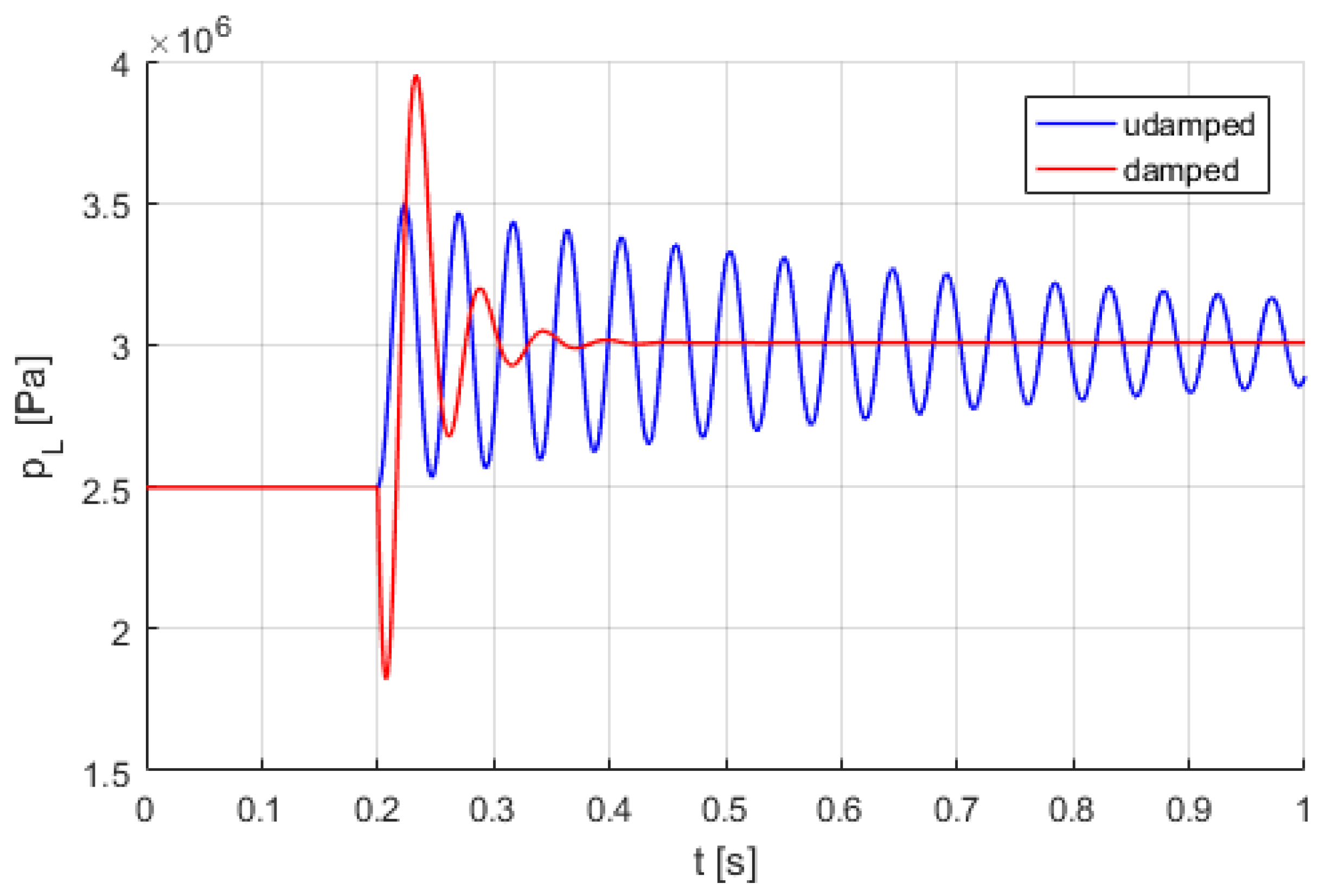
The comparison of the dynamic responses of the undamped and damped shock pressure p_L(t) of an SHA for y_s = 0.6 m and the shock force F = 1000 N is shown in Figure 13. In Figure 13, it can be seen that after using the HSD, a strong damping of the pressure shock is achieved. The higher peak pressure observed in the response characteristic with damping is due to disturbance of the flow during opening of the damping valve.

The dynamic nature of RBS operations involves different values of the shock force acting on the supporting platform. The comparison of the dynamic responses of the shock pressure p_L(t) of an SHA damped by an HSD with different shock forces F is shown in Figure 14. The graph in Figure 14 shows that HSD effectively damps the pressure shocks inducted by shock loads of varying intensity. However, the greater the shock force, the greater the overshoot of the peak pressure and the longer the decay time of the pressure pulsation.

The dynamic response of the shock pressure p_L(t) of an SHA damped by an HSD with the shock force F of irregular appearance is shown in Figure 15.

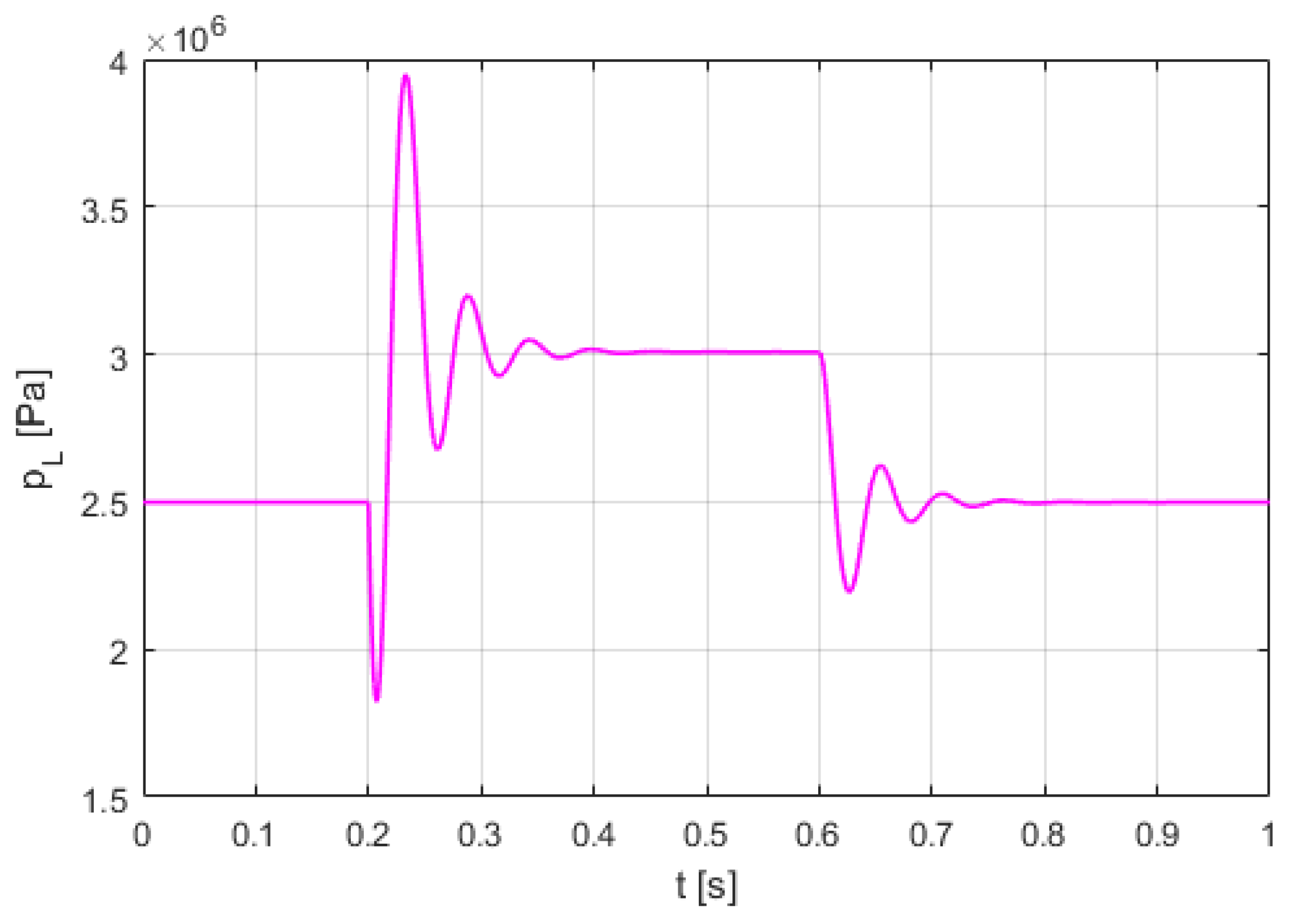
And the dynamic response of the shock pressure p_L(t) of an SHA damped by an HSD for the instantaneous rise and fall shock force F is shown in Figure 16. Instantaneous shock forces at undefined time intervals will be taken into account in the controller of an SHA-HSD system.

5. Implementation of the LQG Controller for an SHA-HSD Control System

The linear quadratic Gaussian (LQG) controller is used for optimal control, the goal of which is to minimize the quadratic cost function subject to the linear system dynamics. The LQG model is used when there is Gaussian noise in the control system and measurement output, and the full state of the system may not be directly observed. The LQG controller combines a linear square controller (LQR) with a Kalman filter (KF), that is, the linear square estimator (LQE) [18,19,20]. The use of the LQG controller makes it possible to take into account the disturbances that occur in the control system and the measuring system. The LQG controller is widely used in vibration control systems, such as semiactive suspensions in sedan cars and multi-axle vehicles [21,22,23]. LQG controllers can also be found in many applications of servo-hydraulic systems [24,25] and the Steward–Gough servo-pneumatic platform [26].

During the bricklaying process, the support legs of the HLL module are locked. The dynamic movement of the loaded and sloped robot arm causes shock loading of the RBS and SHA. An adjustable HSD was used for effective stabilization of the robot platform. For the SHA-HSD system, it is necessary to use a controller that will cause a quick response of the damping valve and effective continuous control of the pressure shock damping. Such requirements are fulfilled by the LQG controller which, after reading the output signal y_m from a position transducer and p_m from a pressure transducer, sets the control input signal u to the switch of the damping valve. The schematic diagram of the LQG controller for an SHA-HSD control system is shown in Figure 17.

The dynamic model (47) of an SHA-HSD system was written as a discrete-time linear state-space model;

$$\{\begin{array}{l}\mathbf{x}(k+1)=A\hspace{0.17em}\mathbf{x}(k)+B\hspace{0.17em}\mathbf{u}(k)\\ \mathbf{y}(k)=C\hspace{0.17em}\mathbf{x}(k)\end{array}$$

(51)

where $x\left(k\right)\in {\mathit{\Re }}^n$ is the state vector, $y\left(k\right)\in {\mathit{\Re }}^p$ is the output vector, $u\left(k\right)\in {\mathit{\Re }}^m$ is the input vector, $A\in {\mathit{\Re }}^{p+n}$ is the state matrix, $B\in {\mathit{\Re }}^{p+n}$ is input matrix, $C\in {\mathit{\Re }}^{p+n}$ is the output matrix, k is discrete time, and t = k T_p, T_p is the sampling time.

The task is to design the LQR control to minimize the quadratic cost function,

$$J={\displaystyle \sum _{k=0}^{\infty }\left[{{\displaystyle \mathbf{x}}}^T(k)\hspace{0.17em}Q\hspace{0.17em}\mathbf{x}(k)+{{\displaystyle \mathbf{u}}}^T(k)\hspace{0.17em}R\hspace{0.17em}\mathbf{u}(k)\right]}$$

(52)

where $Q\in {\mathit{\Re }}^{n+n}$ is the weighting matrix for the states, and $R\in {\mathit{\Re }}^{n+n}$ is the weighting matrix for the control input.

The optimal discrete-time control law is a linear function of the state vector provided by the formula;

$$u(k)=-K\hspace{0.17em}x(k)$$

(53)

where K is the feedback gain matrix that minimizes the quadratic cost function (52).

Substituting (53) into the quadratic cost function (52) provides

$$J(x)=\hspace{0.17em}{\displaystyle \sum _{k=0}^{\infty }{{\displaystyle \mathbf{x}}}^T(k)\left[\hspace{0.17em}Q\hspace{0.17em}+{{\displaystyle K}}^{T}R\hspace{0.17em}K\right]\hspace{0.17em}x(k)}$$

(54)

The optimal feedback gain matrix K is determined by [27],

$$K={{\displaystyle \left({{\displaystyle B}}^T\hspace{0.17em}P\hspace{0.17em}B+R\right)}}^{-1}\hspace{0.17em}{{\displaystyle B}}^T\hspace{0.17em}P\hspace{0.17em}A$$

(55)

where P is the positive definite solution of the discrete algebraic Riccati equation (DARE).

$${{\displaystyle A}}^{T}PA-P\hspace{0.17em}-\hspace{0.17em}\left({{\displaystyle A}}^{T}PB\right){{\displaystyle \left({{\displaystyle B}}^{T}P\hspace{0.17em}B+R\right)}}^{-1}{{\displaystyle B}}^{T}PA\hspace{0.17em}+Q=0$$

(56)

In the case of the LQR controller, the initial weights Q and R can be selected based on the Bryson rule [28]. According to the Bryson rule, Q and R are diagonal matrices whose diagonal elements are expressed, respectively, as the reciprocals of the squares of the maximum acceptable values of the state variable (x) and the input control variable (u).

The diagonal elements Q_ii of matrix Q can be written as

$${{\displaystyle Q}}_{ii}=\frac{1}{\max \left({{\displaystyle x}}_i^2\right)}\hspace{0.17em},\hspace{0.17em}i=1,\dots ,{{\displaystyle n}}_x$$

(57)

where: x_i is the maximum acceptable values of the i-th state variable.

The diagonal elements R_jj of matrix R can be written as

$${{\displaystyle R}}_{jj}=\frac{1}{\max \left({{\displaystyle u}}_j^2\right)}\hspace{0.17em},\hspace{0.17em}j=1,\dots ,{{\displaystyle n}}_u$$

(58)

where u_j is the maximum acceptable values of the j-th control signal.

In the case of an SHA-HSD system with external shock loads, gain matrices Q and R were achieved, with the following values;

$$Q=\left[\begin{array}{cccccc}1& 0& 0& 0& 0& 0\\ 0& 0.1& 0& 0& 0& 0\\ 0& 0& 0.01& 0& 0& 0\\ 0& 0& 0& 0.01& 0& 0\\ 0& 0& 0& 0& 1& 0\\ 0& 0& 0& 0& 0& 0.01\end{array}\right],\hspace{1em}R=\left[1\right].$$

(59)

In order for the controller to be able to follow a reference vector y_r(k), the control law (53) can be rewritten as

$$u(k)=-K\hspace{0.17em}x(k)+{{\displaystyle K}}_r\hspace{0.17em}{{\displaystyle y}}_r(k)$$

(60)

where K_r is the reference gain matrix.

After substituting (60) into (51), it is obtained;

$$\{\begin{array}{l}\mathbf{x}(k+1)=\hspace{0.17em}\left(A\hspace{0.17em}-B\hspace{0.17em}K\right)\mathbf{x}(k)+\hspace{0.17em}B\hspace{0.17em}{{\displaystyle K}}_r{{\displaystyle \mathbf{y}}}_r(k)\\ {{\displaystyle \mathbf{y}}}_r=C\hspace{0.17em}\mathbf{x}(k)\end{array}$$

(61)

From (61), the reference gain matrix K_r was calculated;

$${{\displaystyle K}}_r={{\displaystyle \left[C\hspace{0.17em}{{\displaystyle \left(I-A+B\hspace{0.17em}K\right)}}^{-1}B\right]}}^{-1}$$

(62)

Since z is considered the LQG controller with state estimation using the KF, the linear model of the state space in discrete time has been written in the form;

$$\{\begin{array}{l}\mathbf{x}(k+1)=A\hspace{0.17em}\mathbf{x}(k)+B\hspace{0.17em}\mathbf{u}(k)+G\hspace{0.17em}\mathsf{\psi }(k)\\ {{\displaystyle \mathbf{y}}}_m(k)=H\hspace{0.17em}\mathbf{x}(k)+\mathsf{\theta }\left(k\right)\end{array}$$

(63)

where $y_m\left(k\right)\in {\mathit{\Re }}^p$ is the output measurement vector, ψ is the random Gaussian noise vector (system noise) with zero mean and covariance Qn, G is the transition matrix of the system noise, H is the measurement matrix, and θ is the measurement noise vector with zero mean and known covariance Rn.

In order for the LQG controller to follow two measurement signals, the control law applies;

$$u(k)=-K\hspace{0.17em}\widehat{x}(k)+{{\displaystyle K}}_m\hspace{0.17em}{{\displaystyle y}}_m(k)$$

(64)

where K_m is the measurement gain matrix and y_m(k) is the measurement vector.

The state parameter is obtained from (63) and (64) in the form;

$$x(k)=\hspace{0.17em}\left[A\hspace{0.17em}+B\left({{\displaystyle K}}_m\hspace{0.17em}H-K\right)\right]x(k-1)-B\hspace{0.17em}K\hspace{0.17em}e(k-1)+{{\displaystyle W}}_1$$

(65)

where W₁ is the disturbance matrix,

$${{\displaystyle W}}_1=G\hspace{0.17em}\mathsf{\psi }(k)+B\hspace{0.17em}{{\displaystyle K}}_m\hspace{0.17em}\mathsf{\theta }(k)$$

(66)

The equations of the KF algorithm are divided into two main groups, the time update equations (predictor equations) and measurement update equations (corrector equations). The first group of the KF algorithm is the update of the state and the error covariance according to the following equations;

$$\widehat{x}(k/k-1)=A\hspace{0.17em}\widehat{x}(k-1/k-1)+B\hspace{0.17em}u(k-1)$$

(67)

$$P(k/k-1)=\hspace{0.17em}A\hspace{0.17em}P(k-1/k-1)\hspace{0.17em}{{\displaystyle A}}^T+Qn$$

(68)

where $\widehat{x}$ is the state vector estimator, and P is the covariance of the estimation error. The second group of the KF is the measurement update equations from the sensors which are as follows;

$$\widehat{x}(k/k)=\widehat{x}(k/k-1)+{{\displaystyle K}}_F\hspace{0.17em}\left[y(k)-H\hspace{0.17em}\widehat{x}(k/k-1)\right]$$

(69)

$${{\displaystyle K}}_F=P(k/k-1)\hspace{0.17em}{{\displaystyle H}}^T{{\displaystyle \left[H\hspace{0.17em}P(k/k-1)\hspace{0.17em}{{\displaystyle H}}^T+Rn\right]}}^{-1}$$

(70)

$$P(k/k)=(I-{{\displaystyle K}}_F\hspace{0.17em}H)\hspace{0.17em}P(k/k-1)$$

(71)

where K_F is the KF gain, and I is identity matrix.

For KF tuning, the Qn and Rn noise covariance matrices are used, which directly affect the quality of the state estimation. The process and measurement noises ψ(k) and θ (t) are uncorrelated zero-mean white-noise processes with known noise covariance matrices;

$$E\left[\mathsf{\psi }\hspace{0.17em}{\mathsf{\psi }}^T\right]=Qn,\hspace{1em}E\left[{\displaystyle \mathsf{\theta }}{{\displaystyle \mathsf{\theta }}}^T\right]=Rn$$

(72)

Since the system has only one process noise input, Qn is a scalar equal to the variance of ψ. Since the system has two output channels with uncorrelated measurement noise, Rn is a diagonal matrix. In practice, the appropriate values for Qn and Rn are determined by measuring the noise properties of the system.

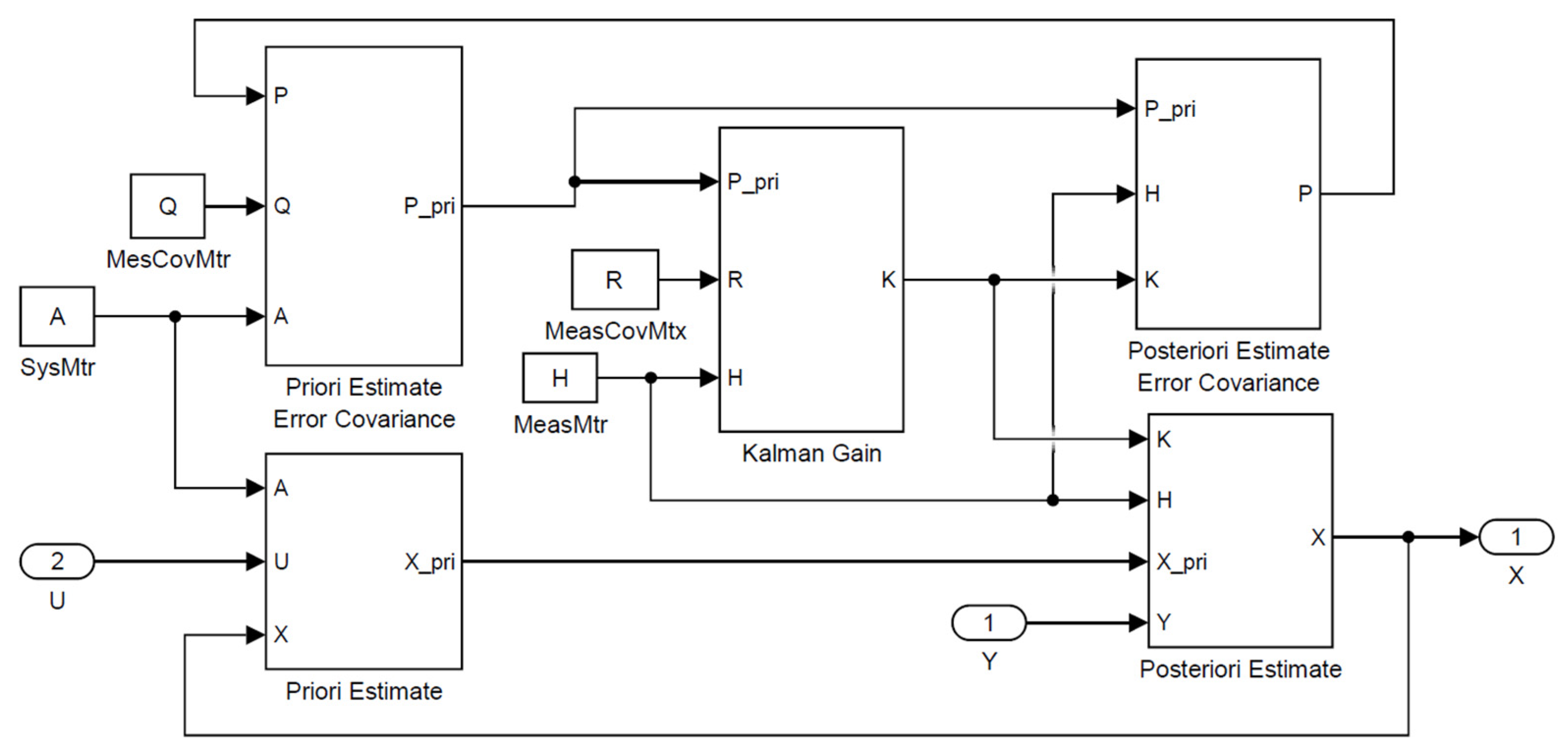
The MATLAB command [KEST,L,P] = kalman(SYS,Qn,Rn) computes the optimal LQG estimator gain for the system model. This command returns the L = K_F gain and the steady-state error covariance matrix P. A large Qn corresponds to little measurement noise and leads to state estimators that respond fast to changes in the measured output. A large Rn corresponds to small disturbances and leads to state-estimates that respond cautiously (slowly) to unexpected changes in the measured output. The discrete KF algorithm of the SHA-HSD system under test is realized in MATLAB/Simulink as seen in Figure 18. In each sub-system, of the time update (predictor) and measurement update (corrector) equations were provided.

The state estimation error can be described as

$$e(k)=x(k)-\widehat{x}(k)$$

(73)

The optimal criterion minimized by the KF algorithm is the sum of the variance of the state estimation errors at each time step k:

$$J(k)=E\left\{{{\displaystyle e(k)}}_1^2\right\}+\cdots +E\left\{{{\displaystyle e(k)}}_n^2\right\}$$

(74)

After substituting (63) and (51) into (73), a state estimation error is obtained in the form of

$$e(k)=\left[A-{{\displaystyle K}}_F\hspace{0.17em}H\right]\hspace{0.17em}e(k-1)+{{\displaystyle W}}_2$$

(75)

where W₂ is the disturbance matrix,

$${{\displaystyle W}}_2=G\hspace{0.17em}\mathsf{\psi }(k)-{{\displaystyle K}}_F\hspace{0.17em}\mathsf{\theta }(k)$$

(76)

The first term of (76) determines the stability properties of the estimation error dynamics, and the second term is the input of external disturbances.

Based on (65) and (75), the dynamics of the feedback loop is written in matrix form;

$$\begin{array}{c}\left[\begin{array}{c}x(k)\\ e(k)\end{array}\right]=\left[\begin{array}{cc}A\hspace{0.17em}+B\left({{\displaystyle K}}_m\hspace{0.17em}H-K\right)& B\hspace{0.17em}K\\ 0& A-{{\displaystyle K}}_F\hspace{0.17em}H\end{array}\right]\left[\begin{array}{c}x(k-1)\\ e(k-1)\end{array}\right]+\left[\begin{array}{c}{{\displaystyle W}}_1\\ {{\displaystyle W}}_2\end{array}\right]=\\ =\left[\begin{array}{cc}Xx& Xw\\ 0& Ew\end{array}\right]\left[\begin{array}{c}x(k-1)\\ e(k-1)\end{array}\right]+\left[\begin{array}{c}{{\displaystyle W}}_1\\ {{\displaystyle W}}_2\end{array}\right]\end{array}$$

(77)

The eigenvalues of matrix (77) were determined from the product of diagonal determinants;

$$\det \left(\lambda I-Xx\right)\hspace{0.17em}\det \left(\lambda I-Ew\right)=0$$

(78)

where λ is the eigenvalue of the matrix block.

Matrices marked by $Xx=A\hspace{0.17em}+B\left({{\displaystyle K}}_m\hspace{0.17em}H-K\right)$, $Xw=B\hspace{0.17em}K$, $Ew=A-{{\displaystyle K}}_F\hspace{0.17em}H$.

Equation (78) shows that the eigenvalues of the controller and the KF estimator are separate from each other in the overall closed-loop LQG system. The principle of separation leads to the conclusion that, for linear time-invariant (LTI) systems, the combination of a stable optimal KF as a state observer with a stable optimal LQR feedback controller allows for an optimal LQG control strategy. The optimality of the closed-loop linear time-invariant system was proved by Tse [29].

The Simulink model of the LQR controller with the KF algorithm of the SHD-HSD system is shown in Figure 19.

6. Control Results

In the SHA-HSD control system, an LQG controller was implemented that follows the measurement parameters (pressure and displacement). The purpose of the LQG controller is to control the shock pressure damping in the HLL module of an RBS. The LQG controller meets the specific requirements of the SHA-HSD system and the nature of the shock loads. Problems with the LQG controller can be due to two possible undesirable characteristics: poor stability margins and poor overall dynamics performance [30]. In the LQG controller, the KF gains were set so that the estimator errors converged long before the controller errors, which should ensure well-preserved feedback properties. The stability margin was improved by influencing the dynamics of the estimator. Control of pressure shock damping was tested with the use of the LQG controller during robotic bricklaying under laboratory conditions.

The experimental study was carried out on a demonstration RBS in laboratory conditions, because it would not be possible to reproduce the shock loads of the brick-laying robot during bricklaying on the test stand. The tests were carried out in various working positions of the bricklaying robot. The tests started with the correct positions of the robot, which required steering the track undercarriage as well as lifting and leveling the RBS. The RBS control system was based on the Simatic HMI (Siemens) operator panel, which consists of several touch screens that can be activated with the appropriate buttons. From the start screen, the touch screen shown in Figure 20 was selected, which was used to control the movement of the track undercarriage and to control the HLL module. Control panel screens can also be operated via the radio console.

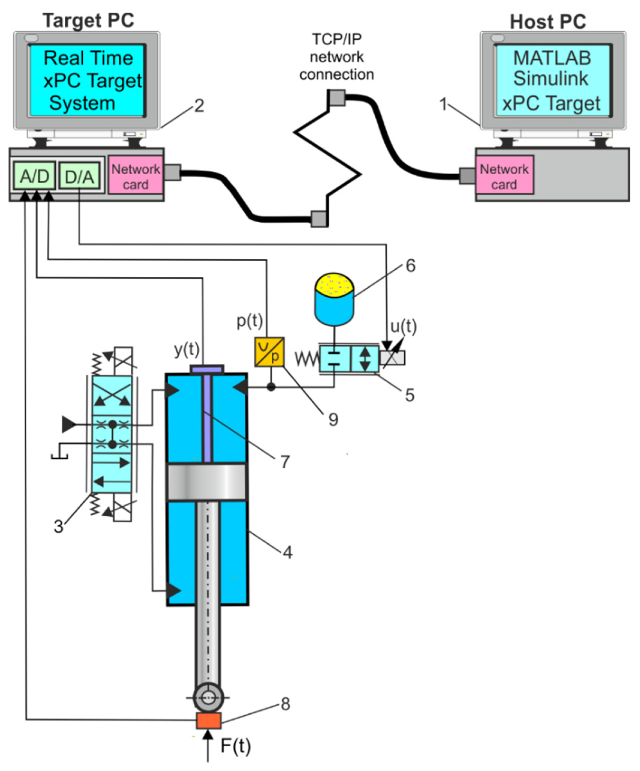
To test the SHA-HSD system, a distributed measurement and control system was used, which consists of the Target PC and the Host PC, where the first PC was the direct control layer, while the second PC acted as the supervisory operator of the control layer. The Host PC and the Target PC communicated with each other via TCP/IP. The computers ran Windows with the MATLAB/Simulink software package. The Target PC had the measurement card (DAS1602 /16–Measurement Computing Corporation) and the Real-Time xPC Target system which was used for measurement data acquisition and control of the damping valve. Simulink, Real-Time Workshop @ and xPC Tar-get software were installed on the host PC. Real-time measurement and control was based on the LQR controller implemented in the Target PC. The measuring transducers were connected to the Target PC via the measuring card. Due to xPC Target Spy software, it is possible to visualize the processed measurement data. The schematic diagram of the distributed measurement and control systems is shown in Figure 21.

The hydraulic actuator has built-in linear position sensors (TMI 0250); transducers that employ the NOVOSTRICTIVE^® touchless magnetostrictive measurement process for direct, precise, and absolute measurement of the linear position in control, positioning, and measuring technology. This transducer provides highly accurate and reliable position control signals and is suitable for demanding industrial (automation) environments. The transducer is equipped with a high dynamic serial DyMoS^® interface with data transmission interface, noncontact guide with a floating position marker, linearity performance up to 30 µm, resolution up to 0.001 mm regardless of stroke length, analog interfaces with teach-in function, low temperature coefficient <20 ppm/K insensitive to shock and vibration, optional cable or plug connection, and protection class IP67/IP68. Furthermore, it is an absolute position transducer and provides a voltage output in the range 0–10 VDC. It requires a supply voltage of 27 VDC and the working pressure is limited to a cylinder chamber pressure of 350 bar.

Pressure is measured by a separate PRW pressure transducer (Peltron). The pressure measurement range is 0–350 bar, the voltage output signal is 0–10 VDC, supplied voltage is 24 VDC, measurement accuracy is ±0.2% FS, measurement time is <1 ms, and the protection class is IP65. The pressure transducer is calibrated using a deadweight pressure tester.

Force is measured using the TecSis3094 force transducer (TecSis). The measurement range of tension and compression force is 0 to 100 kN, voltage output signal is 0–10 VDC, supplied voltage is 12 VDC, measurement accuracy is ±0.15% FS, measurement time is <1 ms, sensitivity is 1.2 mV/V, and the protection class is IP65.

The effectiveness of the LQG controller in the SHA-HSD system was evaluated using the peak pressure overshoot ratio defined as follows:

$${{\displaystyle \delta }}_p=\frac{\Delta p}{{{\displaystyle p}}_{sp}}=\frac{{{\displaystyle p}}_{ps}-{{\displaystyle p}}_{sp}}{{{\displaystyle p}}_{sp}}$$

(79)

where Δp is the overshoot range of the peak pressure, p_ps is the peak pressure, and p_sp is the set pressure.

The peak pressure overshoot ratio for various shock forces was determined in simulation tests and measured during the control of the SHA-HSD system. Figure 22 compares the simulation and the experimental shock pressure ratio for different shock forces.

The experimental results show that the LQG controller in fact damps the shock pressure more effectively than the results from the simulation modelling.

The effectiveness of the LQG controller in damping instantaneous pressure shock in the SHA-HSD system was confirmed by an experiment carried out during RBS bricklaying work under laboratory conditions. The influence of the operation of the LQG controller on the instantaneous pressure shock damping in the SHA-HSD system is shown in an exemplary experimental characteristic Figure 23, obtained from a distributed measurements and control system.

The experimental test confirmed the effectiveness of the discrete LQG controller in controlling the SHA-HSD system because there was no need to correct robot levelling during the bricklaying process.

7. Conclusions

The main goal of the research was achieved, which was stabilization of the leveled position of the RBS subjected to shock loads during automatic RBS operation. Stabilization of the leveled position of the RBS is of great importance for the quality of the bricklaying work performed by the robot, the accuracy of the trajectory path of which depends not only on the mass of bricks carried in the gripper but also on the dynamic loads generated during the movement of the robot manipulator. The presented results of the evaluation of the efficiency of pressure shock damper in the HLL module are part of the mobile RBS tests. The first innovative mobile RBS in Poland was built in cooperation with the industrial partner Strabag Ltd. as a result of a research grant. RBS was successfully tested in laboratory and construction sites, and currently is in the industrial implementation phase.

From a scientific point of view, a new achievement compared with the current state of knowledge resulted in the following development:

• Novel hydraulic shock damping system with adjustable proportional valve that is a semi-active pressure pulsation damper.
• Mathematical transform of the impedance of the damping valve and the impedance of the hydraulic accumulator circuit into the damping efficiency index D(ω) as a quality index (see Equation (34)). The damping efficiency indicators as a function of the frequency ratio are used in the selection of the parameters of the SHA-HSD system due to the effectiveness of pressure shock damping.
• For real-time control of the effectiveness of pressure shock damping in the SHA-HSD system in a distributed measurement and control system, a linear quadratic Gaussian (LQG) controller with the following two measurement signals was implemented;
• To evaluate the effectiveness of the LQG regulator in the SHA-HSD system, a new index was introduced as the peak pressure overshoot ratio.
• The experimental results show that the LQG controller in fact damps the shock pressure more effectively than the results from the simulation modelling.

To fully assess the accuracy of the path of a bricklaying robot, it is necessary to take into account additional parameters of its work, such as mapping the dynamic behavior of the robot at individual points in the bricklaying process. These issues will be the subject of further research, and their results will be presented in subsequent works by the authors.

The presented solution of the SHA-HSD system, confirmed by simulation and experimental results, can be used in various suspension systems for wheeled and tracked heavy vehicles and the supporting systems of mobile cranes, trucks, and crawler cranes. The applied HSD forms a shock pressure damper, which is particularly useful in the hydraulic brake systems of cars because it serves to prevent the transfer of pressure peaks to other wheels. Hydraulic systems employed in earth moving equipment often experience very high input pressure peaks as a result of the forces transmitted to their actuators.

8. Patents

• Utility model Wp.30256 (2021). Tracked transporter. Inventors: Ryszard Dindorf, Jakub Takosoglu, Piotr Wos, Lukasz Chlopek. Kielce University of Technology, Kielce, Poland.
• Utility model Wp.30764 (2022). Tracked transporter housing. Inventors: Ryszard Dindorf, Jakub Takosoglu, Piotr Wos, Lukasz Chlopek. Kielce University of Technology, Kielce, Poland.

References

- Dindorf, R.; Wos, P. A case study of a hydraulic servo drive flexibly connected to a boom manipulator excited by the cyclic impact force generated by a hydraulic rock breaker. IEEE Access 2022, 20, 7734–7752. [Google Scholar] [CrossRef]
- Feng, H.; Du, Q.; Huang, Y.; Chi, Y. Modelling study on stiffness characteristics of the hydraulic cylinder under multifactors. J. Mech. Eng. 2017, 63, 447–456. [Google Scholar] [CrossRef] [Green Version]
- Standard ISO 4413:2010; Hydraulic Fluid Power—General Rules and Safety Requirements for Systems and Their Components. International Organization for Standardization: Geneva, Switzerland, 2010.
- Military Standards: Hydraulic System Components, Ship, Aircraft; U.S. Department of Defense: Washington, DC, USA, 2014.
- Standard ISO 4414:2010; Pneumatic Fluid Power—General Rules and Safety Requirements for Systems and Their Components. International Organization for Standardization: Geneva, Switzerland, 2010.
- Smith, D.J. Reliability, Maintainability and Risk; Butterworth-Heinemann: Oxford, UK, 2001. [Google Scholar]
- Book, W.J. Recursive Lagrangian dynamics of flexible manipulator arms. Int. J. Rob. Res. 1984, 3, 87–101. [Google Scholar] [CrossRef]
- Bernzen, W. On vibration damping of hydraulically driven flexible robots. In Proceedings of the 5th IFAC Symposium on Robot Control, Nantes, France, 3–5 September 1997; pp. 677–682. [Google Scholar]
- Pan, W. Methodological Development for Exploring the Potential to Implement On-Site Robotics and Automation in the Context of Public Housing Construction in Hong Kong. Ph.D. Thesis, Lehrstuhl für Baurealisierung und Baurobotik, Technische Universität München, München, Germany, 2020. [Google Scholar]
- Dakhli, Z.; Lafhaj, Z. Robotic mechanical design for brick-laying automation. Cogent Eng. 2017, 4, 1–22. [Google Scholar] [CrossRef]
- Pritschow, G.; Dalacker, M.; Kurz, J.; Gaenssle, M. Technological aspects in the development of a mobile bricklaying robot. In Proceedings of the 12th International Symposium on Automation and Construction (ISARC), Warsow, Poland, 30 May–1 June 1995; pp. 1–8. [Google Scholar]
- Madsen, A.J. The SAM100: Analyzing Labor Productivity; Construction Management Department, California Polytechnic State University: San Luis Obispo, CA, USA, 2019. [Google Scholar]
- Rihani, R.A.; Bernold, L.E. Methods of control for robotic brick masonry. Autom. Const. 1996, 4, 281–292. [Google Scholar] [CrossRef]
- Wos, P.; Dindorf, R.; Takosoglu, J. The electro-hydraulic lifting and leveling system for the bricklaying robot. In Lecture Notes in Mechanical Engineering; Springer: Cham, Switzerland, 2020; pp. 215–227. [Google Scholar]
- Wos, P.; Dindorf, R.; Takosoglu, J. Bricklaying robot lifting and leveling system. Commun. Sci. Lett. Univ. Žilina 2021, 23, B257–B264. [Google Scholar]
- Wos, P.; Dindorf, R. Hydraulic leveling control system technology of bricklaying robot. In Proceedings of the DSTA’2021, Lodz, Poland, 6–9 December 2021; pp. 582–583. [Google Scholar]
- Dindorf, R.; Wos, P. Development of Hydraulic Power Systems; Monograph M72; Kielce University of Technology: Kielce, Poland, 2016. [Google Scholar]
- Sinha, A. Linear Systems Optimal and Robust Control; CRC Press: Now York, NY, USA, 2007. [Google Scholar]
- Priess, M.C.; Conway, R.; Cho, J.; Popovich, J.M.; Radcliffe, C. Solutions to the Inverse LQR Problem with Application to Biological Systems Analysis. IEEE Trans. Control. Syst. Technol. 2015, 23, 770–777. [Google Scholar] [CrossRef] [PubMed] [Green Version]
- Xia, R.; Li, J.; He, J.; Shi, D.; Zhand, Y. Linear-quadratic Gaussian controller for truck active suspension based on cargo integrity. Adv. Mech. Eng. 2015, 7, 1–9. [Google Scholar] [CrossRef] [Green Version]
- Tseng, H.E.; Hrovat, D. State of the art survey: Active and semi-active suspension control. Veh. Syst. Dyn. 2015, 53, 1034–1062. [Google Scholar] [CrossRef]
- Pang, H.; Chen, Y.; Chen, J.N.; Liu, X. Design of an LQG controller for active suspension without considering road input signals. Shock Vib. 2017, 2017, 6573567. [Google Scholar] [CrossRef] [Green Version]
- Banavar, R.N.; Aggarwal, V. A loop transfer recovery approach to the control of an electro-hydraulic actuator. Con. Eng. Prac. 1998, 6, 837–845. [Google Scholar] [CrossRef]
- Valilou, S. Nonlinear Model and Control of Electro-Hydraulic Servo Systems. Ph.D. Thesis, Department of Engineering and Applied Science, University of Bergamo, Bergamo, Italy, 2017. [Google Scholar]
- Guo, T.; Wang, B.; Tkachev, A.; Zhang, N. An LQG controller based on real system identification for an active hydraulically interconnected suspension. Math. Prob. Eng. 2020, 4, 1–10. [Google Scholar] [CrossRef]
- Karmjit, G.; Dixon, R.; Pearson, J.T. LQG controller design applied to a pneumatic Stewart-Gough platform. Int. J. Autom. Comput. 2012, 9, 45–54. [Google Scholar]
- Crassidis, J.L.; Junkins, J.L. Optimal Estimation of Dynamic Systems, 2nd ed.; CRC Press: Now York, NY, USA, 2012. [Google Scholar]
- Bryson, A.E.; Ho, Y.-C. Applied Optimal Control: Optimization, Estimation, and Control; Taylor & Francis Group: New York, NY, USA, 1975. [Google Scholar]
- Tse, E. On the optimal control of stochastic linear systems. IEEE Trans. Autom. Control 1971, 16, 776–785. [Google Scholar]
- Doyle, J.C. Guaranteed margins in LQG regulators. IEEE Trans. Autom. Control 1978, 23, 664–665. [Google Scholar] [CrossRef] [Green Version]
Figure 1.
Three-dimensional model of mobile RBS. 1: bricklaying robot; 2: tracked undercarriage; 3: robot base platform; 4: hydraulic lifting and leveling module; 5: brick warehouse with brick feeder; 6: control cabinet; 7: control panel.
Figure 2.
View of the bricklaying process (a), bricklaying robot while laying bricks (b), laying bricks in the wall (c), applying mortar on bricks (d).
Figure 3.
HLL module: (a) view of the extendable supporting leg, (b) technical drawing of the cross system of the hydraulic lifting actuators, 1: hydraulic lifting actuator, 2: supporting leg.
Figure 4.
Schematic diagram of an SHA-HSD system: 1: proportional directional control valve, 2: hydraulic lift actuator, 3: magnetostrictive linear position transducer, 4: pressure transducer, 5: proportional damping valve, 6: connecting tube, 7: hydropneumatic accumulator.
Figure 5.
Characteristics of the HAC impedance amplitude.
Figure 6.
Characteristics of the HAC impedance phase.
Figure 7.
Damping efficiency index for different input voltages u of the damping valve at upstream pressure pA = 1 MPa.
Figure 8.
Damping efficiency index for different upstream pressures pA at the input voltage u = 5 V of the damping valve.
Figure 9.
Marking on the bricklaying robot of the mass loads influencing the forces acting on the hydraulic lifting actuators: (a) top view of the RBS structure, (b) side view of the RBS structure.
Figure 10.
Visualize the robot’s trajectory during bricklaying in RobotStudio (ABB).
Figure 11.
Dynamic responses of the displacement y(t) and speed vy(t) of an undamped SHA.
Figure 12.
Dynamic responses of the displacement y(t) and speed vy(t) of an SHA damped by an HSD.
Figure 13.
Comparison of the dynamic responses of the undamped and damped shock pressure pL(t) of an SHA.
Figure 14.
Comparison of the dynamic responses of the shock pressure pL(t) of an SHA damped by an HSD with different shock force F.
Figure 15.
Comparison of the dynamic responses of the shock pressure pL(t) of an SHA damped by an HSD with the shock force of irregular appearance F.
Figure 16.
Dynamic response of the shock pressure pL(t) of an SHA damped by an HSD with instantaneous rise and fall shock force F.
Figure 17.
Schematic diagram of the LQG controller for an SHA-HSD control system.
Figure 18.
Simulink block diagram of the discrete KF algorithm.
Figure 19.
Simulink model of the SHA-HSD control system.
Figure 20.
Touch screen to control the movement of the track undercarriage and the HLL module: 1: selected touch screen, 2: individual track drive select buttons, 3: extension and insertion of individual supporting legs, 4: lifting and lowering individual supporting legs.
Figure 21.
Schematic diagram of distributed measurement and control system: 1: Host PC, 2: Target PC, 3: proportional directional control valve, 4: hydraulic lift actuator, 5: proportional damping valve, 6: hydropneumatic accumulator, 7: linear position transducer, 8: force transducer, 9: pressure transducer.
Figure 22.
Comparison of the peak pressure overshoot ratio for various shock forces.
Figure 23.
Characteristics of instantaneous pressure shock in the HSD-SDD system.
Publisher’s Note: MDPI stays neutral with regard to jurisdictional claims in published maps and institutional affiliations. |
© 2022 by the authors. Licensee MDPI, Basel, Switzerland. This article is an open access article distributed under the terms and conditions of the Creative Commons Attribution (CC BY) license (https://creativecommons.org/licenses/by/4.0/).
Share and Cite
MDPI and ACS Style
Dindorf, R.; Wos, P. Energy Efficiency of Pressure Shock Damper in the Hydraulic Lifting and Leveling Module. Energies 2022, 15, 4097. https://0-doi-org.brum.beds.ac.uk/10.3390/en15114097
AMA Style
Dindorf R, Wos P. Energy Efficiency of Pressure Shock Damper in the Hydraulic Lifting and Leveling Module. Energies. 2022; 15(11):4097. https://0-doi-org.brum.beds.ac.uk/10.3390/en15114097
Chicago/Turabian StyleDindorf, Ryszard, and Piotr Wos. 2022. "Energy Efficiency of Pressure Shock Damper in the Hydraulic Lifting and Leveling Module" Energies 15, no. 11: 4097. https://0-doi-org.brum.beds.ac.uk/10.3390/en15114097
Note that from the first issue of 2016, this journal uses article numbers instead of page numbers. See further details here.