A Nonstandard Path Integral Model for Curved Surface Analysis

Abstract

The nonstandard finite-difference time-domain (NS-FDTD) method is implemented in the differential form on orthogonal grids, hence the benefit of opting for very fine resolutions in order to accurately treat curved surfaces in real-world applications, which indisputably increases the overall computational burden. In particular, these issues can hinder the electromagnetic design of structures with electrically-large size, such as aircrafts. To alleviate this shortcoming, a nonstandard path integral (PI) model for the NS-FDTD method is proposed in this paper, based on the fact that the PI form of Maxwell’s equations is fairly more suitable to treat objects with smooth surfaces than the differential form. The proposed concept uses a pair of basic and complementary path integrals for H-node calculations. Moreover, to attain the desired accuracy level, compared to the NS-FDTD method on square grids, the two path integrals are combined via a set of optimization parameters, determined from the dispersion equation of the PI formula. Through the latter, numerical simulations verify that the new PI model has almost the same modeling precision as the NS-FDTD technique. The featured methodology is applied to several realistic curved structures, which promptly substantiates that the combined use of the featured PI scheme greatly improves the NS-FDTD competences in the case of arbitrarily-shaped objects, modeled by means of coarse orthogonal grids.

1. Introduction

The nonstandard finite-difference time-domain (NS-FDTD) method is an accurate simulation tool having excellent isotropic propagation characteristics for the numerical electromagnetic wave analysis at a desired frequency [1,2,3,4,5,6,7]. Since its accuracy is ${10}^4$ times higher than that of the FDTD technique [8,9], the NS-FDTD approach is suitable for the precise electromagnetic design of objects with electrically large sizes, such as aircrafts comprising various materials, electronic components, and complex airframe shapes [10,11,12,13]. In general, a typical aircraft size is around $500\mathit{\lambda }-1800\lambda$ at the radar frequency. For such dimensions, the phase error of the FDTD method is $7\lambda -23\lambda$ by the wavelength, $\lambda$, and conversion in a $\lambda /10$-discretized computational domain; namely, a critical discretization error. To mitigate this shortcoming, the NS-FDTD algorithm has shown promising precision and efficiency, particularly along with its diverse improvements [14,15,16,17,18], presented during recent years, which are summarized in

Table 1. Strategy status of the curved surface analysis in the NS-FDTD method (Efficacy: Decreasing rate of the calculation cell number used for the verification of the model in the paper or digest).

Year	Ref.	Model	Improved Point	Efficacy
2004	[14]	2D/staircased	Uniform grid ⇒ 2D subgrid model	25
2007	[15]	2D/staircased	Square grid ⇒ Rectangular grid	20
2011	[6]	2D-3D/staircased	Square/cubic cell ⇒ 2D/3D rectangular cell	4.5
2015	[16]	4D/staircased	Cubic cell ⇒ 4D subgrid model	15
2019	[17]	2D/curved	Square grid ⇒ 2D PI model	100
2020	[18]	3D/curved	Cubic cell ⇒ 3D PI model	216

.

Despite its indubitable advantages, the NS-FDTD scheme discretizes the computational space by means of aggregated orthogonal cells, i.e., via the well-known staircase approximation, just as in the typical FDTD method. Nonetheless, it is common knowledge that the optimal design of a realistic arbitrarily-curved structure necessitates the meticulous modeling of every geometric peculiarity, as well as the detailed characterization of any media interface. When these attributes are to be explored by a staircase time-domain method, such as the NS-FDTD one, the requirement of credible discretizations cannot be, easily, fulfilled, because of its inherent restriction to orthogonal lattices. As a consequence, material boundaries, not aligned to the grid axes, are poorly or even erroneously approximated. To evade these difficulties, an assortment of proficient techniques has been proposed (and summarized in [8]), ranging from curvilinear or nonorthogonal FDTD variations to modified Cartesian and conformal algorithms. Nonetheless, the research on this significant topic is constantly escalating, thus leading to various schemes which offer treatment to many contemporary applications from the microwave and optical regime [19,20,21,22,23,24,25,26,27,28,29,30,31] and paving the way to the trustworthy analysis of many future state-of-the-art scientific fields [32,33,34,35,36,37,38,39,40,41,42,43].

Therefore, the manipulation of arbitrarily-curved surfaces or material interfaces via a staircase model deteriorates the reliability of any FDTD-based approach and, particularly, of the NS-FDTD scheme, whose stencils must be very carefully selected. Apparently, the use of finer lattices cannot alleviate this serious hindrance due to the excessive system requirements and the undue increase in the overall computational burden. On the other hand, the use of subgridding techniques [8,9] could yield potential solutions, however, such schemes (in their original form) are often prone to long-time instabilities or opt for very small time increments. Such issues, and particularly the latter, may be proven prohibitive for the NS-FDTD method in the case of prolonged simulations. Indeed, the Courant–Friedrich–Levy (CFL) criterion that controls the stability of both the FDTD and the NS-FDTD algorithms has been, in spite of its worth, one of the most limiting factors for the modeling of electrically large structures. Therefore, to model the tiny-scale features of curved-shaped surfaces, such as those of an aircraft, the cell size selected should be adequately small, enforcing an upper threshold on the time-step that, in turn, leads to thousands of time iterations for the steady-state. To overcome this shortcoming, the alternating-direction implicit (ADI) [44,45,46,47,48,49,50,51] and the locally one-dimensional (LOD) [52,53,54,55,56,57] time marching concepts have been introduced in the update mechanism of most FDTD-oriented schemes. The resulting approach is a semi-explicit technique which surpasses the CFL limit and can conduct unconditionally stable simulations, on the condition that the numerical dispersion and dissipation errors are carefully taken into account.

Considering the prior aspects and the theoretical establishment of the NS-FDTD method, a promising candidate for the analysis of curved surfaces could be the contour-path (CP) model, based on Ampere’s and Faraday’s laws [8]. The CP scheme can properly treat curved details, not necessarily aligned to an orthogonal grid, because the path integral can adapt to any geometrical shape. Another advantage is the use of coarse grids for the handling of curvatures, which seriously decrease the computational overhead. In fact, since its initial advent, the CP model has notably increased the applicability of the FDTD method. Nonetheless, in the NS-FDTD technique, the CP scheme has not yet been introduced. Such a combination could be, indeed, proven to be of critical importance, since the development of the optimal path’s integral model for the NS-FDTD algorithm is necessary to enhance its accuracy in real-world applications.

In this paper, efficient two-dimensional (2D) and three-dimensional (3D) path integral (PI) forms are introduced for the NS-FDTD method, to facilitate the CP modeling of smooth-surface objects. The new PI model launches two types of integral paths on a square grid for each calculation node [16,17]. These path integrals are optimized in terms of certain parameters via the technique’s numerical dispersion equation. Extensive numerical simulations verify that the PI model has a superior isotropy and calculation accuracy (almost equivalent to those of NS-FDTD) compared with the conventional FDTD method. Specifically, practical applications involve the 2D scattering analysis of a circular perfectly electric conductor (PEC) cylinder and the study of a 3D antenna via a thin wire approximation, accordingly tailored for the requirements of the PI model. These demanding numerical investigations promptly reveal that the featured PI model, acting as a CP scheme, as in the original FDTD approach, can decisively improve the modeling competences and accuracy of the NS-FDTD method, even by means of very coarse-grid discretizations.

2. The 2D Path Integral Form

2.1. Development of the Path Integral Model

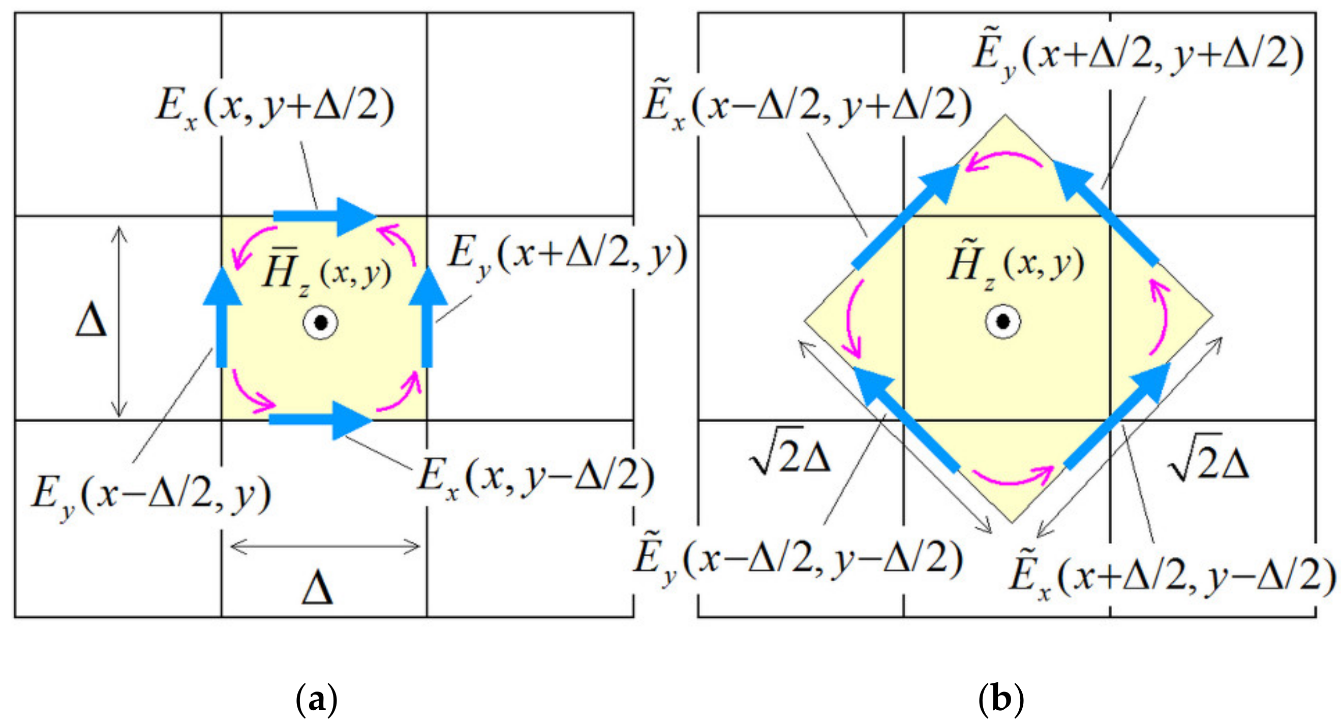
Let us consider a PI model on a square grid, with a cell width $\mathrm{\Delta }$, that offers the highest accuracy for its combined use with the NS-FDTD method. Since, in the conventional FDTD approach, a propagation error arises along the directions of $0^{\circ }$ and ${45}^{\circ }$ on the grid [8], we introduce two distinct integral paths (one rotated ${45}^{\circ }$ with respect to the other) that can mutually cancel their errors, as depicted in Figure 1. In this context, for the basic path (Figure 1a) on a square grid, the integral form of Maxwell’s equations for the $H_z$ magnetic field component is given by

$$\begin{array}{c}\mu {\partial }_t{\displaystyle {\int }_S\mathit{H}\cdot d\mathit{S}}=-{\displaystyle {\int }_l\mathit{E}\cdot d\mathit{l}}\hfill \\ \hfill \Rightarrow \mu {\partial }_t{H}_z^{\mathrm{B}}(x,y){\mathrm{\Delta }}^2=-\left[E_y\left(x+\mathrm{\Delta }/2,y\right)-E_x\left(x,y+\mathrm{\Delta }/2\right)-E_y\left(x-\mathrm{\Delta }/2,y\right)+E_x\left(x,y+\mathrm{\Delta }/2\right)\right]\mathrm{\Delta },\end{array}$$

(1)

while, for the complementary path (Figure 1b),

$$\begin{array}{c}\mu {\partial }_t{\displaystyle {\int }_S\mathit{H}\cdot d\mathit{S}}=-{\displaystyle {\int }_l\mathit{E}\cdot d\mathit{l}}\hfill \\ \hfill \Rightarrow \mu {\partial }_t{H}_z^{\mathrm{C}}(x,y)2{\mathrm{\Delta }}^2=-\left[{\tilde{E}}_y\left(x+\mathrm{\Delta }/2,y+\mathrm{\Delta }/2\right)-{\tilde{E}}_x\left(x-\mathrm{\Delta }/2,y+\mathrm{\Delta }/2\right)\right.\\ \hfill \left. -{\tilde{E}}_y\left(x-\mathrm{\Delta }/2,y-\mathrm{\Delta }/2\right)+{\tilde{E}}_x\left(x+\mathrm{\Delta }/2,y-\mathrm{\Delta }/2\right)\right]\sqrt{2}\mathrm{\Delta }.\end{array}$$

(2)

To guarantee the desired isotropy of the wave propagation on the selected grids, the integral forms of Equations (1) and (2) are combined as

$${\partial }_t{H}_z(x,y)={\beta }_0^{2\mathrm{D}}{\partial }_t{H}_z^{\mathrm{B}}(x,y)+\left(1-{\beta }_0^{2\mathrm{D}}\right){\partial }_t{H}_z^{\mathrm{C}}(x,y),$$

(3)

where ${\beta }_0^{2\mathrm{D}}$ is a parameter, derived in the next subsection, that can finely adjust the overall accuracy of the resulting explicit expressions. Essentially, Equations (1)–(3) constitute the proposed PI model. On the other hand, for the $E_y$ and ${\tilde{E}}_y$ electric field components in Equations (1) and (2), the basic integral path is used as

$$\epsilon {\partial }_t{\displaystyle {\int }_S\mathit{E}\cdot d\mathit{S}}={\displaystyle {\int }_l\mathit{H}\cdot d\mathit{l}}\Rightarrow \epsilon {\partial }_t{E}_y\left(x+\mathrm{\Delta }/2,y\right)=\left[H_z(x,y)-H_z\left(x+\mathrm{\Delta },y\right)\right]/\mathrm{\Delta },$$

(4)

$$\epsilon {\partial }_t{\displaystyle {\int }_S\mathit{E}\cdot d\mathit{S}}={\displaystyle {\int }_l\mathit{H}\cdot d\mathit{l}}\Rightarrow \epsilon {\partial }_t{\tilde{E}}_y(x+\mathrm{\Delta }/2,y+\mathrm{\Delta }/2)=\left[H_z(x,y)-H_z\left(x+\mathrm{\Delta },y+\mathrm{\Delta }\right)\right]/(\sqrt{2}\mathrm{\Delta }),$$

(5)

with analogous expressions holding for the $E_x$ and ${\tilde{E}}_x$ components can, as well. Regarding the PI forms of Equations (1)–(5), the cell width $\mathrm{\Delta }$, the time derivative ${\partial }_{t}g$, and the time increment $\mathrm{\Delta }t$ are substituted by $\mathrm{\Delta }\to s_k(\mathrm{\Delta })=2\sin \left(k\mathrm{\Delta }/2\right)/k$, ${\partial }_{t}g\to \left(g^{t+\mathrm{\Delta }t}-g^t\right)/s_{\omega }(\mathrm{\Delta }t)$ and $\mathrm{\Delta }t\to s_{\omega }(\mathrm{\Delta }t)=2\sin \left(\omega \mathrm{\Delta }t/2\right)/\omega$, respectively, according to the NS-FDTD approach [2,3,4]. Further, $k$ is the wave number and $\omega$ the angular frequency. That is, for (3),

$$\begin{array}{c}\hfill H_z^{t+\mathrm{\Delta }t}(x,y)=H_z^t(x,y)-{\beta }_0^{2\mathrm{D}}\frac{s_{\omega }(\mathrm{\Delta }t)}{\mu s_k(\mathrm{\Delta })}\left[E_y^{t+\mathrm{\Delta }t/2}\left(x+\mathrm{\Delta }/2,y\right)-E_x^{t+\mathrm{\Delta }t/2}\left(x,y+\mathrm{\Delta }/2\right)\right.\\ \hfill \left.-E_y^{t+\mathrm{\Delta }t/2}\left(x-\mathrm{\Delta }/2,y\right)+E_x^{t+\mathrm{\Delta }t/2}\left(x,y-\mathrm{\Delta }/2\right)\right]\\ \hfill -\left(1-{\beta }_0^{2\mathrm{D}}\right)\frac{s_{\omega }(\mathrm{\Delta }t)}{\mu \sqrt{2}{s}_k(\mathrm{\Delta })}\left[{\tilde{E}}_y^{t+\mathrm{\Delta }t/2}\left(x+\mathrm{\Delta }/2,y+\mathrm{\Delta }/2\right)-{\tilde{E}}_x^{t+\mathrm{\Delta }t/2}\left(x-\mathrm{\Delta }/2,y+\mathrm{\Delta }/2\right)\right.\\ \hfill \left.-{\tilde{E}}_y^{t+\mathrm{\Delta }t/2}\left(x-\mathrm{\Delta }/2,y-\mathrm{\Delta }/2\right)+{\tilde{E}}_x^{t+\mathrm{\Delta }t/2}\left(x+\mathrm{\Delta }/2,y-\mathrm{\Delta }/2\right)\right],\end{array}$$

(6)

while the PI expressions of Equations (4) and (5) are obtained by

$$E_y^{t+\mathrm{\Delta }t/2}\left(x+\mathrm{\Delta }/2,y\right)=E_y^{t-\mathrm{\Delta }t/2}\left(x+\mathrm{\Delta }/2,y\right)+\frac{s_{\omega }(\mathrm{\Delta }t)}{\epsilon s_k(\mathrm{\Delta })}\left[H_z^t(x,y)-H_z^t(x+\mathrm{\Delta },y)\right],$$

(7)

$$\begin{array}{c}{\tilde{E}}_y^{t+\mathrm{\Delta }t/2}\left(x+\mathrm{\Delta }/2,y+\mathrm{\Delta }/2\right)={\tilde{E}}_y^{t-\mathrm{\Delta }t/2}\left(x+\mathrm{\Delta }/2,y+\mathrm{\Delta }/2\right)\hfill \\ \hfill +\frac{s_{\omega }(\mathrm{\Delta }t)}{\epsilon \sqrt{2}{s}_k(\mathrm{\Delta })}\left[H_z^t(x,y)-H_z^t\left(x+\mathrm{\Delta },y+\mathrm{\Delta }\right)\right].\end{array}$$

(8)

Similarly, for the $E_x$ and ${\tilde{E}}_x$ components, we arrive at

$$E_x^{t+\mathrm{\Delta }t/2}\left(x,y+\mathrm{\Delta }/2\right)=E_x^{t-\mathrm{\Delta }t/2}\left(x,y+\mathrm{\Delta }/2\right)+\frac{s_{\omega }(\mathrm{\Delta }t)}{\epsilon s_k(\mathrm{\Delta })}\left[H_z^t\left(x,y+\mathrm{\Delta }\right)-H_z^t(x,y)\right],$$

(9)

$$\begin{array}{c}{\tilde{E}}_x^{t+\mathrm{\Delta }t/2}\left(x-\mathrm{\Delta }/2,y+\mathrm{\Delta }/2\right)={\tilde{E}}_x^{t-\mathrm{\Delta }t/2}\left(x-\mathrm{\Delta }/2,y+\mathrm{\Delta }/2\right)\hfill \\ \hfill +\frac{s_{\omega }(\mathrm{\Delta }t)}{\epsilon \sqrt{2}{s}_k(\mathrm{\Delta })}\left[H_z^t\left(x-\mathrm{\Delta },y+\mathrm{\Delta }\right)-H_z^t(x,y)\right].\end{array}$$

(10)

2.2. Derivation of Parameter ${\beta }_0^{2\mathrm{D}}$

To acquire parameter ${\beta }_0^{2\mathrm{D}}$ in Equation (3), let us derive the numerical dispersion equation. Firstly, the monochromatic traveling wave of $g=e^{j(\omega t-k\cdot r)}$ is plugged into Equations (6)–(10), where $j^2=-1$ and $\mathit{r}$ are the position vector, through the analysis of [9]. After some calculus, we define the matrix of the coupled system of equations, for ${\left[E_x,\hspace{0.17em}\hspace{0.17em}{E}_y,\hspace{0.17em}\hspace{0.17em}{\tilde{E}}_y,\hspace{0.17em}\hspace{0.17em}{\tilde{E}}_x,\hspace{0.17em}\hspace{0.17em}{H}_z\right]}^{\mathrm{T}}$, as

$$\mathit{A}=\left[\begin{array}{ccccc}\epsilon W& 0& 0& 0& F_y\\ 0& \epsilon W& 0& 0& -F_x\\ 0& 0& \epsilon W& 0& -S_{\mathrm{A}}\\ 0& 0& 0& \epsilon W& S_{\mathrm{B}}\\ {\beta }_0^{2\mathrm{D}}{F}_y& -{\beta }_0^{2\mathrm{D}}{F}_x& -\left(1-{\beta }_0^{2\mathrm{D}}\right)S_{\mathrm{A}}& \left(1-{\beta }_0^{2\mathrm{D}}\right)S_{\mathrm{B}}& \mu W\end{array}\right],$$

(11)

with

$$W=\sin \left(\omega \mathrm{\Delta }t/2\right)/\mathrm{\Delta }t,k_x=k\cos \theta ,k_y=k\sin \theta ,$$

(12)

$$F_x=\sin \left(k_x\mathrm{\Delta }/2\right)/\mathrm{\Delta },F_y=\sin \left(k_y\mathrm{\Delta }/2\right)/\mathrm{\Delta },$$

(13)

$$S_{\mathrm{A}}=\sin \left(k_x\mathrm{\Delta }/2+k_y\mathrm{\Delta }/2\right)/\sqrt{2}\mathrm{\Delta },S_{\mathrm{B}}=\sin \left(-k_x\mathrm{\Delta }/2+k_y\mathrm{\Delta }/2\right)/\sqrt{2}\mathrm{\Delta }.$$

(14)

Then, the desired numerical dispersion equation is retrieved by imposing the $\det \left\{\mathit{A}\right\}=0$ condition [9], which yields

$$-\epsilon \mu W^2+{\beta }_0^{2\mathrm{D}}\left(F_y^2+F_x^2\right)+\left(1-{\beta }_0^{2\mathrm{D}}\right)\left(S_{\mathrm{A}}^2+S_{\mathrm{B}}^2\right)=0.$$

(15)

Since, for $k=\omega \sqrt{\epsilon \mu },$ parameter ${\beta }_0^{2\mathrm{D}}$ receives its optimal value for every propagation angle $\theta ,$ we substitute the specific $k$ into Equation (15) and solve it with regard to ${\beta }_0^{2\mathrm{D}}$. These algebraic manipulations result in

$${\beta }_0^{2\mathrm{D}}=\left(\epsilon \mu W^2-S_{\mathrm{A}}^2-S_{\mathrm{B}}^2\right)/\left(F_x^2+F_y^2-S_{\mathrm{A}}^2-S_{\mathrm{B}}^2\right),$$

(16)

which, after the use of the appropriate Taylor series for the $\sin \theta$ terms, provides the compact and convenient formula of

$${\beta }_0^{2\mathrm{D}}\approx 2/3-{(k\mathrm{\Delta })}^2/90.$$

(17)

2.3. Numerical Accuracy of the 2D PI Model

Taking into account Equation (15), we numerically examine the accuracy of our PI model with regard to parameter ${\beta }_0^{2\mathrm{D}}$ of Equation (17). The calculated numerical wavenumber, $k_{\mathrm{num}}$, is shown in Figure 2, where the overall error is normalized to the theoretical wavenumber, $k$, in free space, as $\left(k_{\mathrm{num}}-k\right)/k$. In particular, Figure 2a compares the FDTD method, the NS-FDTD technique, and the new PI model, whereas Figure 2b presents a detail of the previous comparison between the NS-FDTD method and the featured PI model. In all simulations, we have selected a wavelength of $\lambda =1$. As promptly observed, the propagation accuracy of our PI model is almost equivalent to that of the original NS-FDTD technique and almost ${10}^4$ times higher than that of the FDTD approach [8]. Consequently, it can be deduced that the PI model is satisfactorily precise to connect with the NS-FDTD scheme. It is stressed that in the next section, we demonstrate the usefulness of the PI scheme, in terms of the prior property, in NS-FDTD regions, so that it can be successfully applied to the treatment of arbitrarily-curved surfaces. Finally, regarding the selection of $\mathrm{\Delta }t$ and based on the FDTD scheme [3,4,5,6,7,8,9], we apply—without loss of generality—the stability condition of $\mathrm{\Delta }t\le \mathrm{\Delta }/(c\sqrt{2}),$ with $\sqrt{2}\mathrm{\Delta }\le \lambda /8$ and $c$ the wave phase velocity, since the proposed 2D PI model uses $\mathrm{\Delta }$- and $\sqrt{2}\mathrm{\Delta }$- width cells simultaneously, as shown in Figure 1.

3. Numerical Verification of the 2D PI Model

In this section, we investigate the efficiency of the proposed 2D PI model. Thus, as an example, let us consider the radar cross section (RCS) of an infinite circular perfectly electric conductor (PEC) cylinder. The PI model, applied on the arbitrary surface, is designated as CP (contour path) in the FDTD algorithm. Therefore, we also use the CP term to refer to the modified PI model, which conforms to curved-surface structures.

3.1. CP Formulation through the Proposed 2D PI Model

For the realization of the PI scheme, in order to effectively model arbitrary surfaces, the modified basic and complementary paths are depicted in Figure 3. Specifically, the integral area for the computation of the $H_z$ magnetic field component is enclosed by two paths, i.e., the $S_B$ and $S_C$ paths, apart from the PEC cylinder area. It should be mentioned that the treatment of the prior CP integrals is based on the same principles as those of the FDTD algorithm. Hence, the integral CP form for the basic path in Figure 3a becomes

$$\begin{array}{c}\mu {\partial }_t{\displaystyle {\int }_{S_{\mathrm{B}}}\mathit{H}\cdot d\mathit{S}}=-{\displaystyle {\int }_l\mathit{E}\cdot d\mathit{l}}\Rightarrow \mu {\partial }_t{H}_z^{\mathrm{B}}(x,y){S^{\prime }}_B{\mathrm{\Delta }}^2\hfill \\ \hfill =E_x\left(x,y+\mathrm{\Delta }/2\right)\mathrm{\Delta }-E_y\left(x+\mathrm{\Delta }/2,y\right)\mathrm{\Delta }+E_y\left(x-\mathrm{\Delta }/2,y\right)l_y\mathrm{\Delta }-E_x\left(x,y-\mathrm{\Delta }/2\right)l_x\mathrm{\Delta },\end{array}$$

(18)

where ${S^{\prime }}_B=S_B/{\mathrm{\Delta }}^2$ and $l_{x,y}=l_{\mathrm{path}\mathrm{length}}/\mathrm{\Delta }$. Actually, this process is the same for the case of the complementary path with an area of $S_C$ in Figure 3b. The treatment for the corresponding $H_z$ formula is also similar to those of Equations (3) and (6), whereas, at the final step of Equation (18), $\mathrm{\Delta }$ is replaced with $s_k(\mathrm{\Delta })=2\sin \left(k\mathrm{\Delta }/2\right)/k$. Observe that, due to the lack of $H_z$ nodes in the PEC area, $E_{x,y}$ and ${\tilde{E}}_{x,y}$ electric field components exist on an integral path which cannot be manipulated via Equations (7)–(10). In such a case, the projection or extrapolation values, obtained from the already extracted $E$ field components at the nearest-neighbor nodes, are utilized. Lastly, the remaining $E$ and $H$ components are derived through the PI Equations (6)–(10).

3.2. Scattering Analysis of a Circular PEC Cylinder

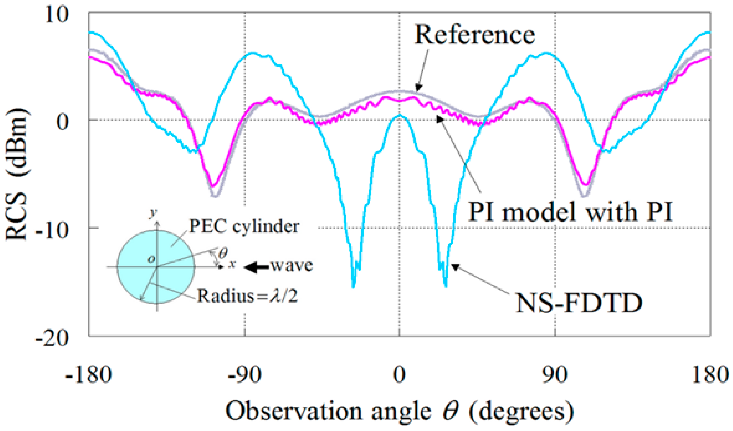
Based on the above aspects, the developed CP model is validated through the RCS evaluation of an infinite circular PEC cylinder with a radius of $\lambda /2$. To this aim, Figure 4 shows the entire computational domain, where the excitation is a TE plane wave with $\lambda =1$ m and an incident angle of ${\theta }^{\mathrm{inc}}=0^{°}$. The scattered field is acquired through the total-field/scattered-field (TF/SF) formulation [8] in the NS-FDTD region. A significant asset of the featured PI concept is its ability to reliably employ coarse grids. Therefore, the CP model uses a spatial increment of $\mathrm{\Delta }=\lambda /12$ for the basic path and a $\lambda /8\ge \sqrt{2}\mathrm{\Delta }$ for the complementary path. Furthermore, the temporal increment is set to $\mathrm{\Delta }t=T/17,$ with $T=2\pi /\omega$. For comparison, the corresponding NS-FDTD simulation is also conducted in the absence of the combined CP and PI model. Figure 5 presents the RCS of the cylinder, where the FDTD results, computed via a staircase model with the much finer resolution of $\mathrm{\Delta }=\lambda /120$ and $\mathrm{\Delta }t=T/170,$ are also given as a reference. Analyzing the outcomes, it is found that our concept agrees very well with both the reference and the NS-FDTD solution. On the other hand, the accuracy of the NS-FDTD method with the resolution of $\mathrm{\Delta }=\lambda /12$ is much lower than that of the featured model.

It should be, additionally, emphasized that the combined CP and PI model succeeds in reducing the overall system requirements to the ${(12/120)}^2=1/100,$ regarding the number of cells, and the ${(12/120)}^2(17/170)=1/1000,$ regarding the time steps, of the respective non-CP case. Consequently, the new PI concept notably enhances the NS-FDTD calculation accuracy, convergence, and overall efficiency for the treatment of curved objects. The small fluctuation of the RCS in Figure 5 depends on the geometric precision of the CP cells at the cylinder surface, as shown in Figure 3, such as the path length and the integral area. This implies that in order to avoid such minor issues, the CP cell model of the curved surfaces must be meticulously designed and implemented.

4. The 3D Path Integral Form

4.1. Development of the Path Integral Model

To derive the 3D extension of our PI concept and cancel the propagation error due to angle dependence, we adopt one basic and one complementary integral path at the $z$ plane and two complementary integral paths at the $z\pm \mathrm{\Delta }$ planes (one rotated ${45}^{\circ }$ with respect to the other), as shown in Figure 6. Therefore, for the basic path at the $z$ plane (on a square grid), the integral form for the $H_z$ magnetic field component is given by

$$\begin{array}{c}\mu {\partial }_t{\displaystyle {\int }_S\mathit{H}\cdot d\mathit{S}}=-{\displaystyle {\int }_l\mathit{E}\cdot d\mathit{l}}\Rightarrow \mu {\partial }_t{H}_z^{\mathrm{B}}\left(x,y,z\right){\mathrm{\Delta }}^2\hfill \\ \hfill =-\left[E_y\left(x+\mathrm{\Delta }/2,y,z\right)-E_x\left(x,y+\mathrm{\Delta }/2,z\right)-E_y\left(x-\mathrm{\Delta }/2,y,z\right)+E_x\left(x,y-\mathrm{\Delta }/2,z\right)\mathrm{\Delta }\right],\end{array}$$

(19)

whereas for the complementary paths at the $z$ and $z\pm \mathrm{\Delta }$ planes, we obtain the form of

$$\begin{array}{c}\mu {\partial }_t{\displaystyle {\int }_S\mathit{H}\cdot d\mathit{S}}=-{\displaystyle {\int }_l\mathit{E}\cdot d\mathit{l}}\hfill \\ \hfill \Rightarrow \mu {\partial }_t{H}_z^{\mathrm{C}}\left(x,y,z\right)2{\mathrm{\Delta }}^2=-\left[{\tilde{E}}_y\left(x+\mathrm{\Delta }/2,y+\mathrm{\Delta }/2,z\right)-{\tilde{E}}_x\left(x-\mathrm{\Delta }/2,y+\mathrm{\Delta }/2,z\right)\right.\\ \hfill \left.-{\tilde{E}}_y\left(x-\mathrm{\Delta }/2,y-\mathrm{\Delta }/2,z\right)+{\tilde{E}}_x\left(x+\mathrm{\Delta }/2,y-\mathrm{\Delta }/2,z\right)\right]\sqrt{2}\mathrm{\Delta },\end{array}$$

(20)

In order to accomplish high isotropy, we use four integral forms, such as those provided in Equations (19) and (20), and derive

$$\begin{array}{c}{\partial }_t{H}_z\left(x,y,z\right)={\beta }_1\left[{\beta }_0{\partial }_t{H}_z^{\mathrm{B}}\left(x,y,z\right)+\left(1-{\beta }_0\right){\partial }_t{H}_z^{\mathrm{C}}\left(x,y,z\right)\right]\hfill \\ \hfill +\left(1-{\beta }_1\right)\left[{\partial }_t{H}_z^{\mathrm{C}}\left(x,y,z+\mathrm{\Delta }\right)+{\partial }_t{H}_z^{\mathrm{C}}\left(x,y,z-\mathrm{\Delta }\right)\right]/2,\end{array}$$

(21)

with ${\beta }_{0,1}$ as the parameters for the 3D isotropic wave propagation, whose optimal values are derived in the next subsection. Actually, Equations (19)–(21) constitute the featured 3D PI form.

Probing further in Equation (20) and through Figure 6, ${\tilde{E}}_y$ may be computed in terms of

$$\begin{array}{c}\epsilon {\partial }_t{\tilde{E}}_y\left(x+\mathrm{\Delta }/2,y+\mathrm{\Delta }/2,z\right)\sqrt{2}{\mathrm{\Delta }}^2=\left[H_z\left(x,y,z\right)-H_z\left(x+\mathrm{\Delta },y+\mathrm{\Delta },z\right)\right]\mathrm{\Delta }\hfill \\ \hfill +\left[{\tilde{H}}_x\left(x+\mathrm{\Delta }/2,y+\mathrm{\Delta }/2,z+\mathrm{\Delta }/2\right)-{\tilde{H}}_x\left(x+\mathrm{\Delta }/2,y+\mathrm{\Delta }/2,z-\mathrm{\Delta }/2\right)\right]\sqrt{2}\mathrm{\Delta },\end{array}$$

(22)

at the $z$ and $z\pm \mathrm{\Delta }$ planes. Likewise, ${\tilde{H}}_x$, in Equation (22), is given by

$$\begin{array}{c}{\tilde{H}}_x\left(x+\mathrm{\Delta }/2,y+\mathrm{\Delta }/2,z\pm \mathrm{\Delta }/2\right)=0.5\left[H_x\left(x+\mathrm{\Delta }/2,y,z\pm \mathrm{\Delta }/2\right)+H_x\left(x+\mathrm{\Delta }/2,y+\mathrm{\Delta },z\pm \mathrm{\Delta }/2\right)\right.\\ \hfill \left.+H_y\left(x,y+\mathrm{\Delta }/2,y,z\pm \mathrm{\Delta }/2\right)+H_y\left(x+\mathrm{\Delta },y+\mathrm{\Delta }/2,z\pm \mathrm{\Delta }/2\right)\right]\cos (\pi /4),\end{array}$$

(23)

where the $\cos (\pi /4)$ term signifies the projection along the ${\tilde{E}}_x$ direction and the $0.5$ refers to the average of the $H_x$ or $H_y$ magnetic field component at the $z\pm \mathrm{\Delta }/2$ planes, for instance, $H_x\left(y+\mathrm{\Delta }/2\right)=0.5\left[H_x(y)+H_x\left(y+\mathrm{\Delta }\right)\right]$. Note that a similar procedure, such as (19)–(23), holds for the evaluation of the $H_x$ and $H_y$ components. On the other hand, regarding the $E_x$ and $E_y$ expressions, we employ the integral path concept on a $\mathrm{\Delta }\times \sqrt{2}\mathrm{\Delta }$ lattice. The final PI formula is acquired by plugging Equations (19), (20), (22), and (23) into (21).

4.2. Derivation of Parameters ${\beta }_0$ and ${\beta }_1$

For the optimal ${\beta }_0$ and ${\beta }_1$ values, let us derive the numerical dispersion equation. Hence, using the trial wave solution in [8,9], Equation (20) leads to

$$\mu {\partial }_t{H}_z^{\mathrm{C}}\left(x,y,z\right)\sqrt{2}\mathrm{\Delta }=2j\sin \left(k_x\mathrm{\Delta }/2+k_y\mathrm{\Delta }/2\right){\tilde{E}}_y\left(x,y,z\right)-2j\sin \left(-k_x\mathrm{\Delta }/2+k_x\mathrm{\Delta }/2\right){\tilde{E}}_x\left(x,y,z\right),$$

(24)

with an analogous expression derived for Equation (19). Moreover, from Equations (19)–(23), we define $\mathit{A}$ as the matrix of the coupled equation set for ${\left[E_x,E_y,E_z,{\tilde{E}}_y^{xy},{\tilde{E}}_x^{xy},{\tilde{E}}_z^{yz},{\tilde{E}}_y^{yz},{\tilde{E}}_z^{xz},{\tilde{E}}_x^{xz},H_x,H_y,H_z\right]}^T$, where superscripts $xy,yz,$ and $xz$ define the plane where $\tilde{E}$ exists. In this manner, the required numerical dispersion equation [8] of our 3D PI model can be extracted from

$$\det \left\{\mathit{A}\right\}=0\iff A_0\left(A_1{A}_2-A_3{A}_4\right)+B_0\left(B_1{B}_2-B_3{B}_4\right)-C_0\left(C_1{C}_2-C_3{C}_4\right)=0,$$

(25)

with coefficients $A_i,B_i,C_i$, for $i=0,1,2,3,4$, elaborately provided in Appendix A.

Subsequently, we determine ${\beta }_0$ and ${\beta }_1$ by considering a plane wave propagating along the $\theta ={90}^{\circ }$ direction at the $xy$ plane. This case is, essentially, the same as the 2D PI model of Equation (3), i.e.,

$${\partial }_t{H}_z\left(x,y,z\right)={\beta }_{{}_0}^{2\mathrm{D}}{\partial }_t{H}_z^{\mathrm{B}}\left(x,y,z\right)+\left(1-{\beta }_{{}_0}^{2\mathrm{D}}\right){\partial }_t{H}_z^{\mathrm{C}}\left(x,y,z\right).$$

(26)

Therefore, comparing Equation (21) with Equation (26), we arrive at

$${\beta }_1{\beta }_0={\beta }_0^{2\mathrm{D}}.$$

(27)

Substituting Equation (27) into Equation (25) and setting $\theta ,\varphi =\pi /4$, as a typical propagation angle, one gets

$$c_{11}{\beta }_1^2+c_{22}{\beta }_1+c_{33}=0,$$

(28)

in which coefficients $c_{11},c_{22}$, and $c_{33}$ are given in Appendix B. Finally, solving Equation (28), the analytical value of ${\beta }_1$ is found to be

$${\beta }_1=\frac{-c_{22}\pm \sqrt{c_{22}^2-4c_{11}{c}_{33}}}{2c_{11}},$$

(29)

while, from Equations (17), (27), and (29), ${\beta }_0$ reads

$${\beta }_0={\beta }_0^{2\mathrm{D}}/{\beta }_1.$$

(30)

4.3. Numerical Accuracy of the 3D PI Model

The propagation accuracy of the novel 3D PI model combined with the NS-FDTD technique is investigated through the numerical dispersion of Equation (25), and the results are illustrated in Figure 7, where the analytical ${\beta }_1$ values are obtained by means of Equation (29) as

$$\mathrm{\Delta }=\lambda /12\Rightarrow {\beta }_1=0.8384\hspace{0.17em}\hspace{0.17em}\hspace{0.17em}\mathrm{a}\mathrm{n}\mathrm{d}\hspace{0.17em}\hspace{0.17em}\hspace{0.17em}0.8297,$$

(31)

$$\mathrm{\Delta }=\lambda /16\Rightarrow {\beta }_1=0.8317\hspace{0.17em}\hspace{0.17em}\hspace{0.17em}\mathrm{a}\mathrm{n}\mathrm{d}\hspace{0.17em}\hspace{0.17em}\hspace{0.17em}0.8313,$$

(32)

$$\mathrm{\Delta }=\lambda /20\Rightarrow {\beta }_1=0.8323\hspace{0.17em}\hspace{0.17em}\hspace{0.17em}\mathrm{a}\mathrm{n}\mathrm{d}\hspace{0.17em}\hspace{0.17em}\hspace{0.17em}0.8320.$$

(33)

It should be mentioned that, after the appropriate study, we found that four mantissa digits were enough for the precise representation of ${\beta }_1$. Furthermore, for the sake of comparison, the regular NS-FDTD outcomes are also plotted in Figure 7, with $k_{\mathrm{num}}$ extracted through the Newton–Raphson method applied to Equation (25). As can be detected from Figure 7, the proposed PI model offers a high propagation accuracy that is almost the same as the one of the NS-FDTD algorithm toward the axial direction of $\varphi =0^{\circ }$. In this way, the propagation error of the NS-FDTD method is in the order of ${10}^{-7}$–${10}^{-8}$, as presented in Figure 8.

Moreover, Figure 9 presents the propagation error of the FDTD method combined with our PI model. Even though the error of the PI model slightly increases at $\varphi ={45}^{\circ }$, it is still three orders of magnitude lower than that of the FDTD method for the same $\mathrm{\Delta }$. Regarding the error fluctuation at $\varphi ={45}^{\circ }$ in the PI results, we can deduce that the error compensation of the PI model was not so sufficient at the $z\pm \mathrm{\Delta }$ planes. Thus, it is proven that the new 3D PI model overwhelms the typical NS-FDTD method in terms of isotropic propagation. Note that in this paper, we use the stability condition of $\mathrm{\Delta }t\le \mathrm{\Delta }/(c\sqrt{3})$ with $\sqrt{2}\mathrm{\Delta }\le \lambda /8,$ since the 3D PI model uses $\mathrm{\Delta }$- and $\sqrt{2}\mathrm{\Delta }$-size cells at the same time, as shown in Figure 6.

5. Numerical Validation of the 3D PI Model

For the certification of the 3D PI model, we analyze the input impedance of a thin wire dipole antenna using the $1/r$ approximation approach [8,59].

5.1. Study of the Thin Wire Antenna Model

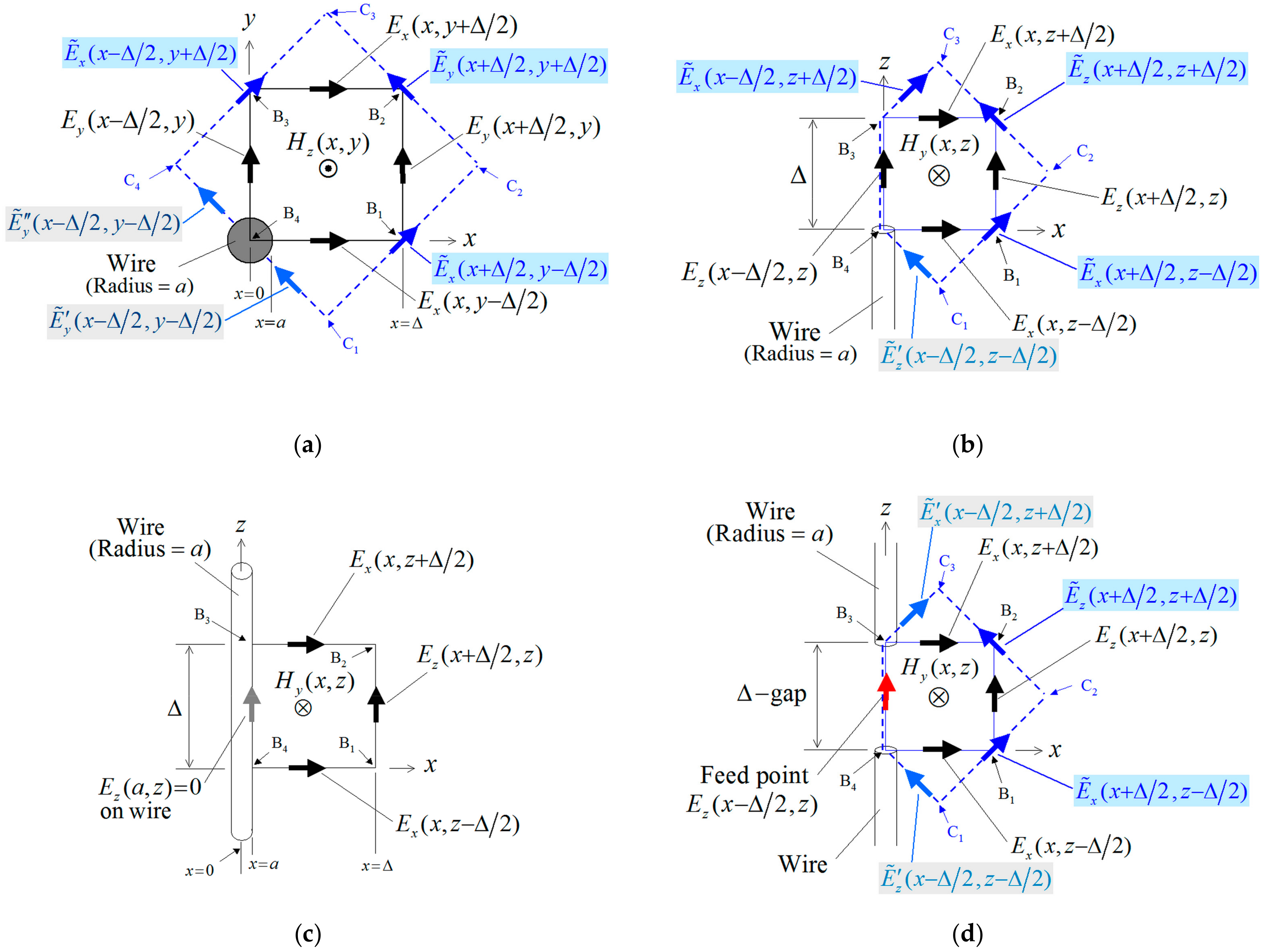
Firstly, we apply the $1/r$ thin wire model for the FDTD method to the 3D PI model. The details of the wire antenna given in Figure 10, where the solid black line refers to the basic path and the dashed blue line to the modified complementary path. Moreover, S_B is the area enclosed by the basic path and S_C the respective area for the complementary path. In this framework, the integral area for ${\partial }_t{\displaystyle {\mathrm{\int }}_S\mathit{H}\cdot d\mathit{S}}$ is: S_B =${\mathrm{\Delta }}^2-\pi a^2/4$ and S_C =$2{\mathrm{\Delta }}^2$$-\pi a^2/2$ in Figure 10a; S_B =${\mathrm{\Delta }}^2$ and S_C =$7{\mathrm{\Delta }}^2/4-a^2/2$ in Figure 10b; S_B =${\mathrm{\Delta }}^2-a\mathrm{\Delta }$ in Figure 10c; and S_B =${\mathrm{\Delta }}^2$ and S_C =$7{\mathrm{\Delta }}^2/4-a^2$ in Figure 10d.

In particular, for the complementary path in Figure 10a,

$${{\tilde{E}}^{\prime }}_y\left(x-\mathrm{\Delta }/2,y-\mathrm{\Delta }/2\right)=\left[E_x\left(x,y-\mathrm{\Delta }/2\right){\mathit{e}}_x+E_y\left(x-\mathrm{\Delta }/2,y-\mathrm{\Delta }\right){\mathit{e}}_y\right]\cdot \mathit{t},$$

(34)

$${{\tilde{E}}^{″}}_y\left(x-\mathrm{\Delta }/2,y-\mathrm{\Delta }/2\right)=\left[E_x\left(x-\mathrm{\Delta },y-\mathrm{\Delta }/2\right){\mathit{e}}_x+E_y\left(x-\mathrm{\Delta }/2,y\right){\mathit{e}}_y\right]\cdot \mathit{t},$$

(35)

where $\mathit{t}=\left(-{\mathit{e}}_x+{\mathit{e}}_y\right)/\sqrt{2}$ and ${\mathit{e}}_x,{\mathit{e}}_y$ are the unit vectors. Since, in the above expressions, $E_x\left(x,y-\mathrm{\Delta }/2\right)\propto 1/x$ and $E_y\left(x-\mathrm{\Delta }/2,y\right)\propto 1/y$, we obtain

$$\begin{array}{c}{\displaystyle {\int }_{{\mathrm{C}}_1}^{{\mathrm{C}}_4}\tilde{\mathit{E}}\cdot d\mathit{l}}={\displaystyle {\int }_a^{\sqrt{2}\mathrm{\Delta }/2}\sqrt{2}\mathrm{\Delta }{{\tilde{E}}^{\prime }}_y\left(x-\mathrm{\Delta }/2,y-\mathrm{\Delta }/2\right)/(2l)}dl+{\displaystyle {\int }_a^{\sqrt{2}\mathrm{\Delta }/2}\sqrt{2}\mathrm{\Delta }{{\tilde{E}}^{″}}_y\left(x-\mathrm{\Delta }/2,y-\mathrm{\Delta }/2\right)/(2l)}dl\hfill \\ \hfill =(\mathrm{\Delta }/\sqrt{2})\ln (\mathrm{\Delta }/\sqrt{2}a)\left[{\widetilde{E^{\prime }}}_y\left(x-\mathrm{\Delta }/2,y-\mathrm{\Delta }/2\right)+{\widetilde{E^{″}}}_y\left(x-\mathrm{\Delta }/2,y-\mathrm{\Delta }/2\right)\right].\end{array}$$

(36)

On the other hand, for the complementary path in Figure 10b,d, we get

$${{\tilde{E}}^{\prime }}_z\left(x-\mathrm{\Delta }/2,z-\mathrm{\Delta }/2\right)=-E_x\left(x,z-\mathrm{\Delta }/2\right)\cos (\pi /4),$$

(37)

$${{\tilde{E}}^{\prime }}_x\left(x-\mathrm{\Delta }/2,z+\mathrm{\Delta }/2\right)=E_x\left(x,z+\mathrm{\Delta }/2\right)\cos (\pi /4),$$

(38)

where $E_x\left(x,y\pm \mathrm{\Delta }/2\right)\propto 1/x,$ except the $E_x\left(x,y+\mathrm{\Delta }/2\right)$ term in Figure 10b. Hence,

$${\displaystyle {\int }_{{\mathrm{C}}_1}^{{\mathrm{B}}_4}{\tilde{\mathit{E}}}^{\prime }\cdot d\mathit{l}=}{\displaystyle {\int }_{\sqrt{2}a}^{\sqrt{2}\mathrm{\Delta }/2}\sqrt{2}\mathrm{\Delta }{{\tilde{E}}^{\prime }}_y\left(x-\mathrm{\Delta }/2,y-\mathrm{\Delta }/2\right)}/(4l)dl=\sqrt{2}\mathrm{\Delta }\ln \left(\mathrm{\Delta }/2a\right){\widetilde{E^{\prime }}}_y\left(x-\mathrm{\Delta }/2,y-\mathrm{\Delta }/2\right)/4,$$

(39)

$${\displaystyle {\int }_{{\mathrm{B}}_3}^{{\mathrm{C}}_3}{\tilde{\mathit{E}}}^{\prime }\cdot d\mathit{l}=}{\displaystyle {\int }_{\sqrt{2}a}^{\sqrt{2}\mathrm{\Delta }/2}\sqrt{2}\mathrm{\Delta }{{\tilde{E}}^{\prime }}_x\left(x-\mathrm{\Delta }/2,y+\mathrm{\Delta }/2\right)}/(4l)dl=\sqrt{2}\mathrm{\Delta }\ln \left(\mathrm{\Delta }/2a\right){\widetilde{E^{\prime }}}_x\left(x-\mathrm{\Delta }/2,y+\mathrm{\Delta }/2\right)/4.$$

(40)

Additionally, for the basic path in Figure 10a, it is derived that

$${\displaystyle {\int }_{{\mathrm{B}}_4}^{{\mathrm{B}}_1}\mathit{E}\cdot d\mathit{l}=}{\displaystyle {\int }_a^{\mathrm{\Delta }}\mathrm{\Delta }{E}_x\left(x,y-\mathrm{\Delta }/2\right)}/(2l)dl=\mathrm{\Delta }\ln \left(\mathrm{\Delta }/a\right)E_x\left(x,y-\mathrm{\Delta }/2\right)/2,$$

(41)

with a similar treatment holding for the integral paths ${\mathrm{B}}_4-{\mathrm{B}}_3$ in Figure 10a, ${\mathrm{B}}_4-{\mathrm{B}}_1$ in Figure 10b–d, and ${\mathrm{B}}_3-{\mathrm{B}}_2$ in Figure 10c,d. Regarding the surface integral of ${\partial }_t{H}_y$ in Figure 10c, we employ the basic path and acquire

$${\partial }_t{\displaystyle {\int }_S{H}_y^{\mathrm{B}}}dS\Rightarrow {\partial }_t{H}_y^{\mathrm{B}}(x,z)={\mathrm{\Delta }}^2\ln \left(\mathrm{\Delta }/2a\right)/2,$$

(42)

where $H_y\propto 1/x$. It should be stressed that all integral calculations, apart from Equations (34)–(42), treat the field value on the path as a constant. To calculate the ${\partial }_t{H}_y$ and ${\partial }_t{H}_z$, we use Equations (34)–(42) in Equation (21), considering $\mu {\partial }_t{\displaystyle {\int }_S\mathit{H}\cdot d\mathit{S}}=-{\displaystyle {\int }_l\mathit{E}\cdot d\mathit{l}}$ and having replaced $\mathrm{\Delta }$ with $s_k(\mathrm{\Delta })$. Finally, for the ${\partial }_t\mathit{E}$ term, the basic integral path is utilized. Note that the feed point with a $\mathrm{\Delta }$ gap at $E_z\left(x-\mathrm{\Delta }/2,z\right)$, shown in Figure 10d, is evaluated by means of

$${\displaystyle {\int }_S\left(\epsilon {\partial }_t\mathit{E}+\sigma \mathit{E}+{\mathit{J}}_D\right)\cdot d\mathit{S}}={\displaystyle {\int }_l\mathit{H}\cdot d\mathit{l}},$$

(43)

with $\sigma$ being the electric conductivity and ${\mathit{J}}_D$ the driving current.

5.2. Dipole Antenna Analysis

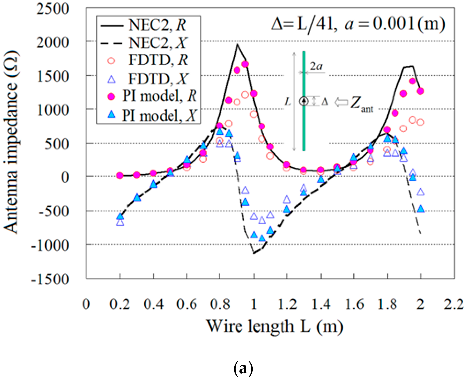
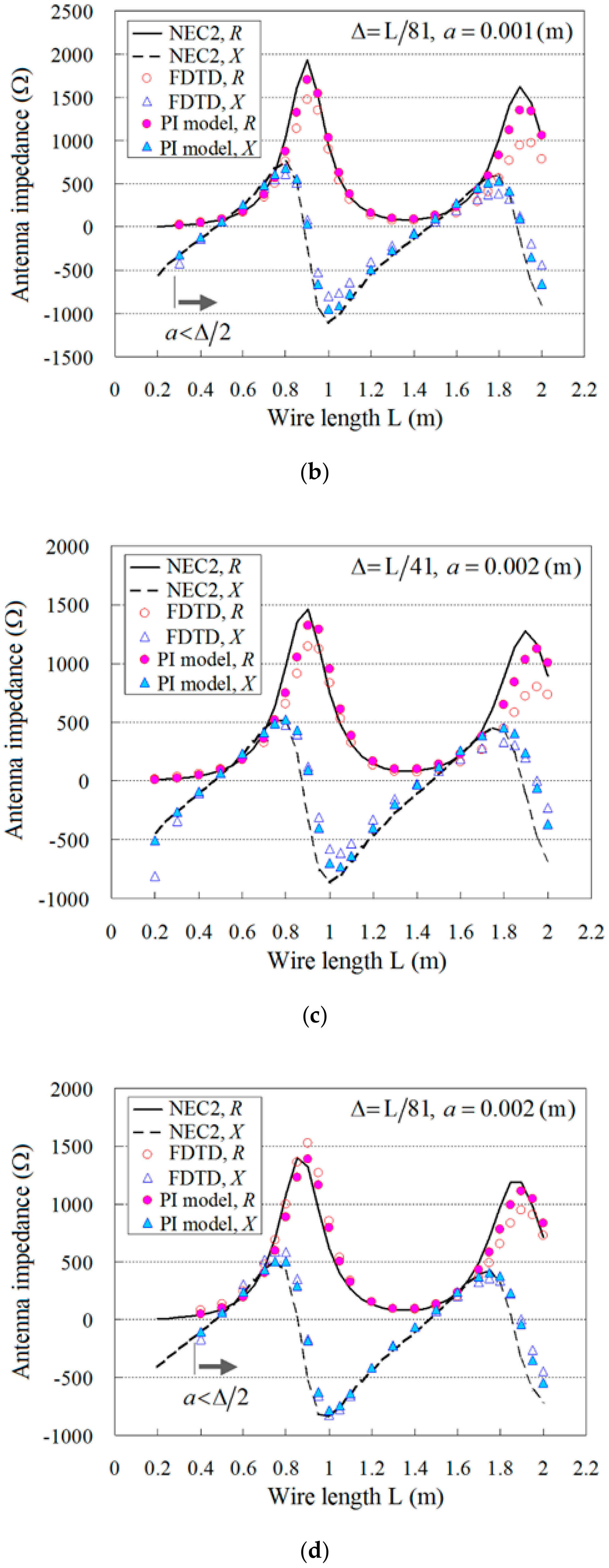
Bearing in mind the above analysis, we study the impedance of a dipole antenna of length $L$, using the modified $1/r$ models for the featured PI scheme, as in Figure 10. The antenna is placed at the center of the PI region of width $10\mathrm{\Delta }$ around the wire. Outside the PI area, we have a $200\mathrm{\Delta }\times 200\mathrm{\Delta }\times 300\mathrm{\Delta }$ NS-FDTD region, terminated with a $20\mathrm{\Delta }$-wide perfectly matched layer (PML) [58]. Figure 11 presents the antenna impedance versus the wire length, with $\lambda =1$ m and $\mathrm{\Delta }=L/N,$ for $N=41$ and $81$. For the selection of the time increment, we employ the stability criterion of the FDTD method. In addition, the antenna is driven by a center feed with a gap $\mathrm{\Delta }$ along the $z$ axis, as shown in Figure 10d, while the evaluated wire radii are $a=0.001$ m and $0.002$ m. As our reference in Figure 11, we use the results retrieved via the Numerical Electromagnetics Code (NEC2) computational package [60], which implements the method of moments [61], whereas the corresponding FDTD results [8] are also provided. Note that the antenna impedance, $Z_{\mathrm{ant}}=R+jX,$ at the feed point is calculated by

$$Z_{\mathrm{ant}}=R+jX=-\frac{{\displaystyle {\int }_{{\mathrm{B}}_4}^{{\mathrm{B}}_3}\mathit{E}\cdot dl}}{{\displaystyle {\int }_l\mathit{H}\cdot dl}},$$

(44)

referring to Figure 10d [59]. In Equation (44), the denominator gives the contour integration of the magnetic field $\mathit{H}$ around the feed point. It can be discerned from Figure 11 that all the outcomes derived via the PI model are in very good agreement with the NEC2 outcomes. Moreover, the PI concept achieves higher accuracy than the typical FDTD method. As a consequence, the modified thin wire antenna model based on the PI scheme is proven to be very efficient, unlike the original NS-FDTD technique in differential form, offering the opportunity for the precise analysis of demanding thin wire structures.

6. Conclusions

A novel PI formulation for the rigorous treatment of curved surfaces on square grids via the 2D and 3D NS-FDTD method has been presented in this paper. In essence, the developed model has been extended to a robust CP scheme, which can enhance the efficiency of the main numerical algorithm, even with coarse mesh tessellations. After the pertinent numerical investigation, it has been confirmed that the PI model exhibits a comparable accuracy and isotropy to the NS-FDTD technique. Moreover, all results obtained from 2D RCS calculations and 3D thin-wire antenna studies substantiated that the PI implementation is fully compatible with all the interfaces of the NS-FDTD domain. Therefore, taking into account that the proposed methodology avoids excessively fine lattices, it can be deemed as a precise and reliable means for modeling electrically-large objects with complex curved surfaces or media interfaces, frequently encountered in the design of modern electromagnetic configurations.

References

- Mickens, R.E. Applications of Nonstandard Finite-Difference Schemes; World Scientific: Singapore, 2000. [Google Scholar]
- Cole, J.B. A high accuracy FDTD algorithm to solve microwave propagation and scattering problems on coarse grid. IEEE Trans. Microw. Theory Tech. 1995, 43, 2053–2058. [Google Scholar] [CrossRef]
- Cole, J.B. A high-accuracy realization of the Yee algorithm using non-standard finite differences. IEEE Trans. Microw. Theory Tech. 1997, 45, 991–996. [Google Scholar] [CrossRef]
- Cole, J.B. High-accuracy Yee algorithm based on nonstandard finite differences: New developments and verifications. IEEE Trans. Antennas Propag. 2002, 50, 1185–1191. [Google Scholar] [CrossRef]
- Ohtani, T.; Kanai, Y. Optimal coefficients of the spatial finite difference operator for the complex nonstandard finite difference time-domain method. IEEE Trans. Magn. 2011, 47, 1498–1501. [Google Scholar] [CrossRef]
- Ohtani, T.; Kanai, Y. Coefficients of finite difference operator for rectangular cell NS-FDTD method. IEEE Trans. Antennas Propag. 2011, 59, 206–213. [Google Scholar] [CrossRef]
- Cole, J.B.; Banerjee, S. Computing the Flow of Light; SPIE Press: Bellingham, WA, USA, 2017. [Google Scholar]
- Taflove, A.; Hagness, S.C. Computational Electrodynamics: The Finite-Difference Time-Domain Method, 3rd ed.; Artech House: Norwood, MA, USA, 2005; Chapters 4, 7, 8, 10. [Google Scholar]
- Kunz, K.S.; Luebbers, R.J. The Finite Difference Time Domain Method for Electromagnetics; CRC Press: New York, NY, USA, 1993; Chapter 17. [Google Scholar]
- Fuhs, A.E. Radar Cross Section Lectures; Naval Postgraduate School (DTIC Accession Number: ADA125576): Monterey, CA, USA, 1982. [Google Scholar]
- de Andrade, L.A.; dos Santos, L.S.C.; Gama, A.M. Analysis of radar cross section reduction of fighter aircraft by means of computer simulation. J. Aerosp. Manag. 2014, 6, 177–182. [Google Scholar]
- Zhou, Z.; Huang, J. Study of the radar cross-section of turbofan engine with biaxial multirotor based on dynamic scattering method. Energies 2020, 13, 5802. [Google Scholar] [CrossRef]
- Alves, Μ.A.; Port, R.J.; Rezende, M.C. Simulation of the Radar Cross Section of a Stealth Aircraft. In Proceedings of the 2007 SBMO/IEEE MTT-S International Microwave and Optoelectronics Conference (IMOC), Salvador, Brazil, 29 October–1 November 2007; pp. 409–412. [Google Scholar]
- Ohtani, Τ.; Taguchi, K.; Kashiwa, T. A subgridding technique for the complex nonstandard FDTD method. Electron. Commun. Jpn. Part 2 2004, 87, 234–241. [Google Scholar] [CrossRef]
- Ohtani, T.; Taguchi, K.; Kashiwa, T.; Kanai, Y. Overlap algorithm for the nonstandard FDTD method using nonuniform mesh. IEEE Trans. Magn. 2007, 43, 1317–1320. [Google Scholar] [CrossRef]
- Ohtani, T.; Kanai, Y.; Kantartzis, N.V. A 4-D subgrid scheme for the NS-FDTD technique using the CNS-FDTD algorithm with the Shepard method and a Gaussian smoothing filter. IEEE Trans. Magn. 2015, 51, 7201004. [Google Scholar] [CrossRef]
- Ohtani, T.; Kanai, Y.; Kantartzis, N.V. A Rigorous Path Integral Scheme for the Two-Dimensional Nonstandard Finite-Difference Time-Domain Method. In Proceedings of the 22nd IEEE Conference on the Computation of Electromagnetic Fields (COMPUMAG), Paris, France, 15–19 July 2019; p. PA-M4-9. [Google Scholar]
- Ohtani, T.; Kanai, Y.; Kantartzis, N.V. An Efficient Contour-Path Integral Model for the 3-D Nonstandard Finite-Difference Time-Domain Technique. In Proceedings of the 19th IEEE Conference on Electromagnetic Field Computation (CEFC), Pisa, Italy, 16–18 November 2020; p. 53. [Google Scholar]
- Li, J.; Tang, Y.; Li, Z.; Ding, X.; Yuan, D.; Yu, B. Study on scattering and absorption properties of quantum-dot-converted elements for light-emitting diodes using finite-difference time-domain method. Materials 2017, 10, 1264. [Google Scholar] [CrossRef] [PubMed] [Green Version]
- Codecasa, L.; Kapidani, B.; Specogna, R.; Trevisan, F. Novel FDTD technique over tetrahedral grids for conductive media. IEEE Trans. Antennas Propag. 2018, 66, 5387–5396. [Google Scholar] [CrossRef]
- Fazio, E.; Alonzo, M.; Belardini, A. Addressable refraction and curved soliton waveguides using electric interfaces. Appl. Sci. 2019, 9, 347. [Google Scholar] [CrossRef] [Green Version]
- Wang, X.; Gao, J.; Teixeira, F.L. Stability-improved ADE-FDTD method for wideband modeling of graphene structures. IEEE Antennas Wirel. Propag. Lett. 2019, 18, 212–216. [Google Scholar] [CrossRef]
- Shibayama, J.; Suzuki, K.; Iwamoto, T.; Yamauchi, J.; Nakano, H. Dispersive contour-path FDTD algorithm for the Drude–Lorentz model. IEEE Antennas Wirel. Propag. Lett. 2020, 19, 1699–1703. [Google Scholar] [CrossRef]
- Navarro, E.A.; Portí, J.A.; Salinas, A.; Navarro-Modesto, E.; Toledo-Redondo, S.; Fornieles, J. Design & optimization of large cylindrical radomes with subcell and non-orthogonal FDTD meshes combined with genetic algorithms. Electronics 2021, 10, 2263. [Google Scholar]
- Ma, X.; Du, B.; Tan, S.; Song, H.; Liu, S. Spectral characteristics simulation of topological micro-nano structures based on finite difference time domain method. Nanomaterials 2021, 11, 2622. [Google Scholar] [CrossRef]
- Baxter, J.; Lesina, A.C.; Ramunno, L. Parallel FDTD modeling of nonlocality in plasmonics. IEEE Trans. Antennas Propag. 2021, 69, 3982–3994. [Google Scholar] [CrossRef]
- Kim, M.; Park, S. Modified finite-difference time-domain method for Hertzian dipole source under low-frequency band. Electronics 2021, 10, 2733. [Google Scholar] [CrossRef]
- Sirvent-Verdú, J.J.; Francés, J.; Márquez, A.; Neipp, C.; Álvarez, M.; Puerto, D.; Gallego, S.; Pascual, I. Precise-integration time-domain formulation for optical periodic media. Materials 2021, 14, 7896. [Google Scholar] [CrossRef]
- Feng, N.; Zhang, Y.; Huang, Z.; Yang, L.; Wu, X. Numerical prediction of duality principle with Bloch-Floquet periodic boundary condition in fully anisotropic FDTD. Remote Sens. 2022, 14, 1135. [Google Scholar] [CrossRef]
- Liu, S.; Tan, E.L.; Zou, B. Incident plane-wave source formulations for leapfrog complying-divergence implicit FDTD method. IEEE J. Multiscale Multiphys. Comput. Tech. 2022, 7, 84–91. [Google Scholar] [CrossRef]
- Mescia, L.; Bia, P.; Caratelli, D. FDTD-based electromagnetic modeling of dielectric materials with fractional dispersive response. Electronics 2022, 11, 1588. [Google Scholar] [CrossRef]
- Devaraj, V.; Lee, J.-M.; Oh, J.-W. Distinguishable plasmonic nanoparticle and gap mode properties in a silver nanoparticle on a gold film system using three-dimensional FDTD simulations. Nanomaterials 2018, 8, 582. [Google Scholar] [CrossRef] [Green Version]
- Loubani, A.; Harid, N.; Griffiths, H.; Barkat, B. Simulation of partial discharge induced EM waves using FDTD method—A parametric study. Energies 2019, 12, 3364. [Google Scholar] [CrossRef] [Green Version]
- Zhang, P.; He, D.; Zhang, C.; Yan, Z. FDTD simulation: Simultaneous measurement of the refractive index and the pressure using microdisk resonator with two whispering-gallery modes. Sensors 2020, 20, 3955. [Google Scholar] [CrossRef]
- Leman, J.T.; Olsen, R.G. Bulk FDTD simulation of distributed Corona effects and overvoltage profiles for HSIL transmission line design. Energies 2020, 13, 2474. [Google Scholar] [CrossRef]
- Ding, X.; Shao, C.; Yu, S.; Yu, B.; Li, Z.; Tang, Y. Study of the optical properties of multi-particle phosphors by the FDTD and ray tracing combined method. Photonics 2020, 7, 126. [Google Scholar] [CrossRef]
- Mohammadi, S.; Karami, H.; Azadifar, M.; Rachidi, F. On the efficiency of OpenACC-aided GPU-based FDTD approach: Application to lightning electromagnetic fields. Appl. Sci. 2020, 10, 2359. [Google Scholar] [CrossRef] [Green Version]
- Fu, Y.; Yager, T.; Chikvaidze, G.; Iyer, S.; Wang, Q. Time-resolved FDTD and experimental FTIR study of gold micropatch arrays for wavelength-selective mid-infrared optical coupling. Sensors 2021, 21, 5203. [Google Scholar] [CrossRef]
- Feng, N.; Zhang, Y.; Wang, G.P.; Zeng, Q.; Joines, W.T. Compact matrix-exponential-based FDTD with second-order PML and direct Z-transform for modeling complex subsurface sensing and imaging problems. Remote Sens. 2021, 13, 94. [Google Scholar] [CrossRef]
- Januszkiewicz, Ł. Analysis of shielding properties of head covers made of conductive materials in application to 5G wireless systems. Energies 2021, 14, 7004. [Google Scholar] [CrossRef]
- Feng, H.; Zhang, Z.; Zhang, J.; Fang, D.; Wang, J.; Liu, C.; Wu, T.; Wang, G.; Wang, L.; Ran, L.; et al. Tunable dual-broadband terahertz absorber with vanadium dioxide metamaterial. Nanomaterials 2022, 12, 1731. [Google Scholar] [CrossRef] [PubMed]
- Wu, T.; Wang, G.; Jia, Y.; Shao, Y.; Gao, Y.; Gao, Y. Dynamic modulation of THz absorption frequency, bandwidth, and amplitude via strontium titanate and graphene. Nanomaterials 2022, 12, 1353. [Google Scholar] [CrossRef]
- Gomez-Cruz, J.; Bdour, Y.; Stamplecoskie, K.; Escobedo, C. FDTD analysis of hotspot-enabling hybrid nanohole-nanoparticle structures for SERS detection. Biosensors 2022, 12, 128. [Google Scholar] [CrossRef]
- Namiki, T.; Ito, K. Investigation of numerical errors of the two-dimensional ADI-FDTD method. IEEE Trans. Microw. Theory Tech. 2000, 48, 1950–1956. [Google Scholar]
- Zheng, F.; Chen, Z.; Zhang, J. A finite-difference time-domain method without the courant stability conditions. IEEE Microw. Guided Wave Lett. 1999, 9, 441–443. [Google Scholar] [CrossRef] [Green Version]
- Venkatarayalu, N.V.; Lee, R.; Gan, Y.-B.; Li, L.-W. A stable FDTD subgridding method based on finite element formulation with hanging variables. IEEE Trans. Antennas Propag. 2007, 53, 907–915. [Google Scholar] [CrossRef]
- Matsuo, T. Electromagnetic field computation using space-time grid and finite integration method. IEEE Trans. Magn. 2010, 46, 3241–3244. [Google Scholar] [CrossRef]
- Maksymov, S.; Sukhorukov, A.A.; Lavrinenko, A.V.; Kivshar, Y.S. Comparative study of FDTD-adopted numerical algorithms for Kerr nonlinearities. IEEE Antennas Wirel. Propag. Lett. 2011, 10, 143–146. [Google Scholar] [CrossRef]
- Feng, N.; Zhang, Y.; Tian, X.; Zhu, J.; Joines, W.T.; Wang, G.P. System-combined ADI-FDTD method and its electromagnetic applications in microwave circuits and antennas. IEEE Trans. Microw. Theory Tech. 2019, 67, 3260–3270. [Google Scholar] [CrossRef]
- Li, Y.; Wang, N.; Lei, J.; Wang, F.; Li, C. Modeling GPR wave propagation in complex underground structures using conformal ADI-FDTD algorithm. Appl. Sci. 2022, 12, 5219. [Google Scholar] [CrossRef]
- Tan, E.L. From time-collocated to leapfrog fundamental schemes for ADI and CDI FDTD methods. Axioms 2022, 11, 23. [Google Scholar] [CrossRef]
- Rana, M.M. Fundamental scheme-based nonorthogonal LOD-FDTD for analyzing curved structures. IEEE Antennas Wirel. Propag. Lett. 2017, 16, 337–340. [Google Scholar] [CrossRef]
- Yan, J.; Jiao, D. An unsymmetric FDTD subgridding algorithm with unconditional stability. IEEE Trans. Antennas Propag. 2018, 66, 4137–4150. [Google Scholar] [CrossRef]
- Moradi, M.; Pourangha, S.-M.; Nayyeri, V.; Soleimani, M.; Ramahi, O.M. Unconditionally stable FDTD algorithm for 3-D electromagnetic simulation of nonlinear media. Opt. Express 2019, 27, 15018–15031. [Google Scholar] [CrossRef]
- Stracqualursi, E.; Araneo, R.; Lovat, G.; Andreotti, A.; Burghignoli, P.; Brandão Faria, J.; Celozzi, S. Analysis of metal oxide varistor arresters for protection of multiconductor transmission lines using unconditionally-stable Crank-Nicolson FDTD. Energies 2020, 13, 2112. [Google Scholar] [CrossRef]
- Kuang, X.; Huang, Z.; Fang, M.; Qi, Q.; Chen, M.; Wu, X. Novel high-order symplectic compact FDTD schemes for optical waveguide simulation. IEEE Photon. J. 2022, 14, 2211407. [Google Scholar] [CrossRef]
- Park, J.; Baek, J.-W.; Jung, K.-Y. Accurate and numerically stable FDTD modeling of human skin tissues in THz band. IEEE Access 2022, 10, 41260–41266. [Google Scholar] [CrossRef]
- Bérenger, J.-P. Perfectly Matched Layer (PML) for Computational Electromagnetics; Morgan & Claypool Publishers: San Rafael, CA, USA, 2007. [Google Scholar]
- Jensen, M.A.; Rahmat-Samii, Y. Performance analysis of antennas for hand-held transceivers using FDTD. IEEE Trans. Antennas Propag. 1994, 42, 1106–1113. [Google Scholar] [CrossRef] [Green Version]
- Numerical Electromagnetics Code (NEC2). Available online: https://www.nec2.org/ (accessed on 1 April 2022).
- Harrington, R.F. Field Computation by Moment Methods; IEEE Press: Piscataway, NJ, USA, 1993. [Google Scholar]
Figure 1.
Integration paths on a square grid for the proposed PI model. (a) Basic path and (b) complementary path. The two paths are rotated , one with respect the other, in order to mutually cancel their errors. Thus, the nodes for the coefficients of the NS-FDTD operators [2,3,4] are not required.
Figure 2.
Numerically computed wavenumber, , versus propagation angle for the FDTD method, the NS-FDTD technique, and the proposed 2D PI model. (a) General comparison and (b) detail of the previous plot only between the NS-FDTD method and the PI model. In the analysis, is the physical wavenumber, the wavelength is chosen to be , is the grid size, and . Note that the NS-FDTD method and the PI model have practically the same accuracy, which is almost four orders of magnitude higher (or even more) than that of the FDTD method.
Figure 3.
Modified integral paths for the proposed PI model based on (Figure 1a) and (Figure 1b), respectively. (a) Basic path and (b) complementary path. Dashed lines represent the position of the pair paths, PEC areas are indicated in light blue, and signifies the ratio of the path length over . Note that the integral path and the area for the calculation of the magnetic field component form a part, except for the PEC region, indicated at the right side of the figure. The treatment of the path integrals in Equations (4) and (5) is based on the same principles as those in the FDTD algorithm.
Figure 4.
The computational domain for the RCS analysis of the infinite circular PEC cylinder with a radius of , concerning the validation of the 2D CP technique applied to the proposed PI concept in the NS-FDTD area terminated by a perfectly matched layer (PML) [58]. The structure is excited by a TE plane wave with m and an incident angle of while all scattered-field components are obtained by means of the TF/SF formulation [8] in the NS-FDTD region.
Figure 5.
RCS results obtained via the FDTD, the NS-FDTD, and the proposed 2D CP model for the computational configuration of Figure 4. The incident angle of the TE plane wave is . Moreover, the FDTD results are obtained with and (via the usual staircase discretization scheme), while the NS-FDTD results (without the CP model) are extracted with .
Figure 6.
The four integral paths for the calculation of the magnetic field component on a square grid (similarly for the and fields). Specifically, we devise one basic and one complementary path at the plane and two complementary paths at the planes in order to cancel the propagation error owing to angle dependence.
Figure 7.
Propagation error of the numerical wavenumber, , obtained via the Newton-Raphson method using Equation (25), for the NS-FDTD method combined with the proposed PI model and (a) , (b) , and (c) . Note that is the grid size, the physical wavenumber, the wavelength, and the angles of the spherical coordinate system . For comparison, the typical NS-FDTD results [6] are also included.
Figure 8.
Propagation error of the numerical wavenumber, , for the NS-FDTD method combined with the proposed PI model. Note that is the grid size, the physical wavenumber, the wavelength, and the angles of the spherical coordinate system . The PI model attains a high propagation accuracy, practically equivalent to that of the NS-FDTD method along the axial direction .
Figure 9.
Propagation error of the numerical wavenumber, , for the FDTD method combined with the proposed PI model. Note that are the angles of the spherical coordinate system . Although the error of the PI model increases at , it remains approximately times lower than that of the FDTD method for the same grid size .
Figure 10.
The proposed PI model for a thin wire antenna of radius . Integral path (a) in the vicinity of the wire at a cross section, (b) for a wire end on the axis, (c) in the vicinity of the wire along the axis (this part uses only the basic path), and (d) for the feed point with a gap on the axis. The black solid line signifies the basic path and dashed blue line the modified complementary path, while, for simplicity, the axis, in (b–d), and the axis, in (a), are omitted. Designating as SB the area enclosed by the basic path and SC the area enclosed by the complementary path, the integral area for is: SB = and SC = for (a); SB = and SC = for (b); SB = for (c); SB = and SC = for (d).
Figure 11.
Antenna impedance, , as in Equation (44), obtained via the proposed PI model, the FDTD method, and NEC2 [60] (reference solution), for m and (a) , m, (b) , m, (c) , m, and (d) , m. Due to the limitations of the approximation model [8,59] on the grid, the extracted results are presented for , apart from those derived via NEC2 [60].