Financial Hazard Assessment for Electricity Suppliers Due to Power Outages: The Revenue Loss Perspective

Abstract

The electrical power infrastructure of the modern world is advanced, efficient, and robust, yet power outages still occur. In addition to affecting millions of people around the world, these outage events cost billions of dollars to the global economy. In this paper, the revenue loss borne by electricity-supplying companies in the United States due to power outage events is estimated and predicted. Various factors responsible for power outages are considered in order to present an exploratory data analysis at the U.S. level, followed by the top ten affected states, which bear over 85% of the total revenue loss. The loss is computed using historic observational data of electricity usage patterns and the tariff offered by the energy suppliers. The study is supplemented with reliable and publicly available records, including electricity usage patterns, the consumer category distribution, climatological annotations, population density, socio-economic indicators and land area. Machine learning techniques are used to predict the revenue loss for future outage events, as well as to characterize the key parameters for efficient prediction and their partial dependence. The results show that the revenue loss is a function of several parameters, including residential sales, percentage of industrial customer, time-period of the year, and economic indicators. This study may help energy suppliers make risk-informed decisions, while developing revenue generation strategies as well as identifying safer investment avenues for long-term returns.

1. Introduction

Power infrastructure reliability and pliability is a major concern worldwide. The modern world demands uninterrupted electric power to fulfill its rapidly increasing needs. The power infrastructure in the United States (U.S.) is classic, complicated, and extensive, spanning over a large geographical area. The existing infrastructure is becoming fragile, but current expansion plans are not enough considering the rising electricity demand [1]. Interruption in the power supply affects everyone, including the utility industry, socio-econometric activities, law and order, and the health and education sectors. There are a number of causes of power outage events in the U.S., such as natural or weather-induced disasters, system operability disruption, equipment failure, fuel supply emergencies, islanding, intentional attacks, and public appeals. However, weather-induced natural disasters have been the top cause of power outage events [2,3]. From the environmental perspective, some areas are more exposed to natural disasters in comparison to others. Shen et al. [4], based on data from 2007 to 2018, revealed that the eastern U.S. is more vulnerable to severe weather disasters. In another study conducting single-state analysis, it was found that Texas (TX), California (CA), and Ohio (OH) were prone to several kinds of weather-induced disasters; Michigan had the highest frequency of disasters, followed by Texas and California; and hurricanes were the most common disaster in Texas, Florida, New York, and Louisiana [5].

The frequency of weather-related natural disasters has significantly increased over the last two decades. Such events are detrimental to the smooth running of electric power systems and may trigger cascaded power outages [3,6,7]. During the current year (2021), Texas faced a major power crisis due to three extreme winter storms that swept across the U.S. [8]. During the year 2020, a total of 22 severe weather and climatological events, such as tropical cyclones, storms, droughts, and wildfire, occurred across the United States [5]; this surpasses the previous record of 16 events, which occurred in both 2011 and 2017 [9]. From 2003 to 2012, the cause of 80% of all outages was severe weather events [10]. A report by the U.S. Department of Energy (DOE) in 2017 showed that more than 90% of power outages occurred in the transmission phase, and most of them were due to extreme weather events.

Power outage events, specifically those due to weather-related natural disasters, not only cause prolonged outages affecting millions of people, but also result in a huge financial loss. The winter storms in 2021 alone cost the U.S. economy a record USD 200 billion [11]. The winter storm that hit Texas in Feb 2021 affected 5 million people, with 151 casualties [12]. According to one estimate, it resulted in a total economic loss of USD 45–50 billion, including the destruction of structures, loss of jobs and wages, medical expenses, and damage to businesses [13]. The 22 disaster events that happened in the year 2020 alone cost more than USD 1 billion per event. The top three of these events included: Hurricane Laura (Category 4) on 27–28 August in Louisiana, which caused a total economic loss of USD 18+ billion; Derecho on 10 August, which traveled from South Dakota to Ohio with a wind speed of 80–100 mph, causing severe damage and a total economic loss of USD 11 billion; and Hurricane Sally (Category 2) on 14–18 September, along the Alabama coast, which saw a record 1–2 feet of rain in Florida and Alabama and caused a total economic loss of USD 7 billion [5]. In 2017 alone, the U.S. witnessed 16 disasters, which cost billions of US dollars [14]. Hurricane Sandy in 2012 affected 8 million people and caused a loss of USD 70 billion [15]. Hurricane Irene in 2011 affected a population of 6 million, with a financial loss of USD 10 billion [15]. From 2003 to 2012, severe-weather-related power outages cost the U.S. economy USD 20 to 50 billion [15]. In the period 1980–2017, weather-induced natural disasters cost the U.S. circa USD 219 billion [16]. Regarding the consequence of power outages, as discussed above, studies have been carried out to assess the overall economic losses caused by these events, including the cost of infrastructure damage, damage to equipment, revenue loss due to non-sale of electricity, costs to consumers due to non-provision of the power supply, and so on. These studies consider two perspectives: one is the (residential/commercial/industrial) consumer’s perspective of monetary loss, which they bear due to the absence of power; and the other is the supplier’s perspective, where he bears the revenue loss due to non-sale of electricity. In our study, we use the data from historical power outage events and aim to specifically compute, as well as predict, the revenue loss borne by electricity suppliers due to non-sale of electricity during such events.

2. Background

The economic loss due to interruption of electricity can be estimated based on the feedback from users. For instance, the estimated financial loss based on the feedback provided by commercial sector users will represent the commercial monetary loss. Similarly, estimates can be made for other sectors by collecting the information from their corresponding consumers. However, this approach is less practical, since most of the time the outage occurs due to natural disasters, so post-event circumstances are difficult, and it is hard to approach and collect feedback from the people affected. Another popular and widely used approach for financial loss assessment is based on how much money the user is willing to pay (WTP) for an uninterrupted supply of electricity [17]. This is a subjective assessment based on individual’s way of thinking and the added value they associate with an uninterrupted supply of electricity. In recent literature, this approach has been extensively used by researchers for economic loss assessment associated with power outages. One study estimated the economic loss from climate change effects using this approach [18]. Research conducted on small firms in Hyderabad, India, revealed how much the owners were willing to pay for a consistent supply of electricity [18]. The authors concluded that, on average, the firms were willing to pay 20% more for an uninterrupted electricity supply. Another study was conducted in Zambia to assess the willingness of organizations to pay for an improvement in the reliability of their electric power supply [19]. It was concluded that large organizations with higher revenues were willing to pay more than small firms for an uninterrupted supply of electricity. Another study from Nepal used the contingent valuation approach to rate the willingness to pay for improved services after the energy crises during 2008–2016 [20]. The authors reported that households were ready to pay an extra 65% of the actual monthly electricity bill for improved quality of power supply. Another study discussed estimates of users’ willingness to pay for developing a local, limited electric power supply system in case of long outages [21]. The study discusses different scenarios based on services during the outage; the duration of supplied services; and the billing cost over 5, 10, and 20 years for the development of a limited power supply system for use during long outages. Another study presents an economic loss assessment based on Pennsylvania residential customers’ willingness to pay for uninterrupted power supply up to 20A for a week-long period [22]. The residents were willing to pay up to USD 1.2 per kWh for their high-priority services.

The studies discussed above used the WTP (willingness to pay) approach and presented the financial loss estimation from consumers’ perspective. However, there is hardly any evidence focusing on the electricity suppliers’ perspective of financial damage; in particular, estimation of the revenue loss incurred by electric supply enterprises due to non-sale of electricity has not been discussed in the past literature, and we are going to explore this aspect.

In general, the economic loss due to interruption of electricity can be estimated in different contexts based on the nature of the collected/available information, as has been presented in the literature [23,24,25,26,27]. Among these studies, many considered the economic loss estimation from the perspective of consumers (for instance, residential, industrial, or commercial consumers). However, the perspective of electric power suppliers regarding fiscal loss in these sectors due to power outages has not been discussed.

There is a significant amount of literature related to the economic loss caused by power outages using the end users’ WTP for ensuring an uninterrupted supply of electricity. Other methods to estimate economic losses were based on post-outage feedback from affected consumers. Again, there is hardly any evidence of revenue loss assessment based on non-sale of electricity itself. Public and private electric-power-supplying enterprises bear a huge revenue loss associated with power outage events. However, there is a gap in the literature to accurately quantify this phenomenon. In this study, the estimation of revenue losses due to power outages borne by electricity suppliers due to non-sale of electricity is presented. For this purpose, a publicly available historical data set for the U.S. is used. The data includes records of electricity usage patterns, socio-economic indicators, the number of consumers belonging to different sectors, the population of individual states, the land area, and so on [28]. A study has already been carried out using this data, where the 10 most vulnerable states of the U.S. were extensively studied [29]. An exploratory data analysis is presented covering the outage events’ frequency, the reasons for occurrence, the natural disaster impact, and the computation of revenue losses due to non-sale of electricity. Machine learning techniques are employed to predict such revenue losses for future outage events. The relation between the revenue loss and the potential parameters for estimation is characterized.

The organization of the rest of the paper is as follows: Section 3 presents the exploratory data analysis. Section 4 explains the methodology. The results and discussion are presented in Section 5. The conclusion is added in Section 6.

3. Exploratory Data Analysis

Comprehensive historical data including several parameters related to power outage events that occurred during 2000–2016 are used. A total of 1534 power outage events occurred from 2000 to 2016 in the US. The data is publicly available and contains the information of 1534 power outage events over a 17-year time period [28]. It includes seven types of events that triggered the power outage. The data includes observations of several parameters recorded at the time of the outage event, which are distributed among nine different categories, where each category includes multiple indicators. The categories of the data and their corresponding sources are shown in

Table 1. Historical data categories and their respective sources [28].

Sr No	Data Category	Data Sources
1	Annual population	U.S. Census Bureau
2	Electricity consumption	National Oceanic and Administrative Administration (NOAA)
3	Percentage of customers	US Energy Information Administration (EIA 826)
4	Economic parameters	Bureau of Economic Analysis
5	Land and water mass percentage	U.S. Census Bureau
6	Climate and water data	NOAA’s National Climate Data Centre (NCDC)
7	Year category	NOAA
8	Regional climate (by state)	NOAA
9	Urban and rural area percentage	U.S. Census Bureau

.

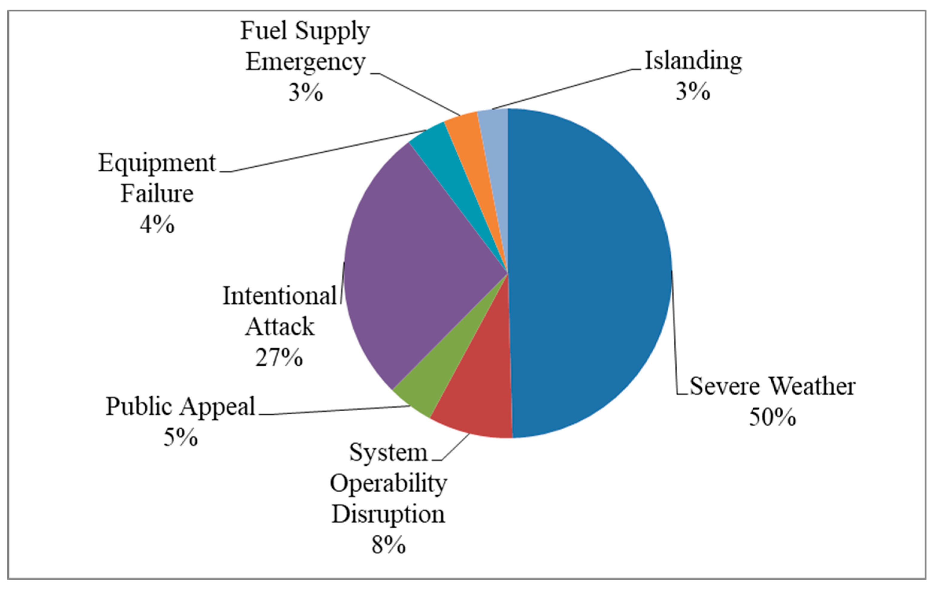
The data reveals that there were seven different types of events that have caused power outages, including severe weather, islanding, fuel supply emergency, equipment failure, system operability disruption, intentional attacks, and public appeal. The frequency of these events is shown as percentages in the Figure 1. It is evident that half of the outage events were triggered by severe-weather-related natural disasters.

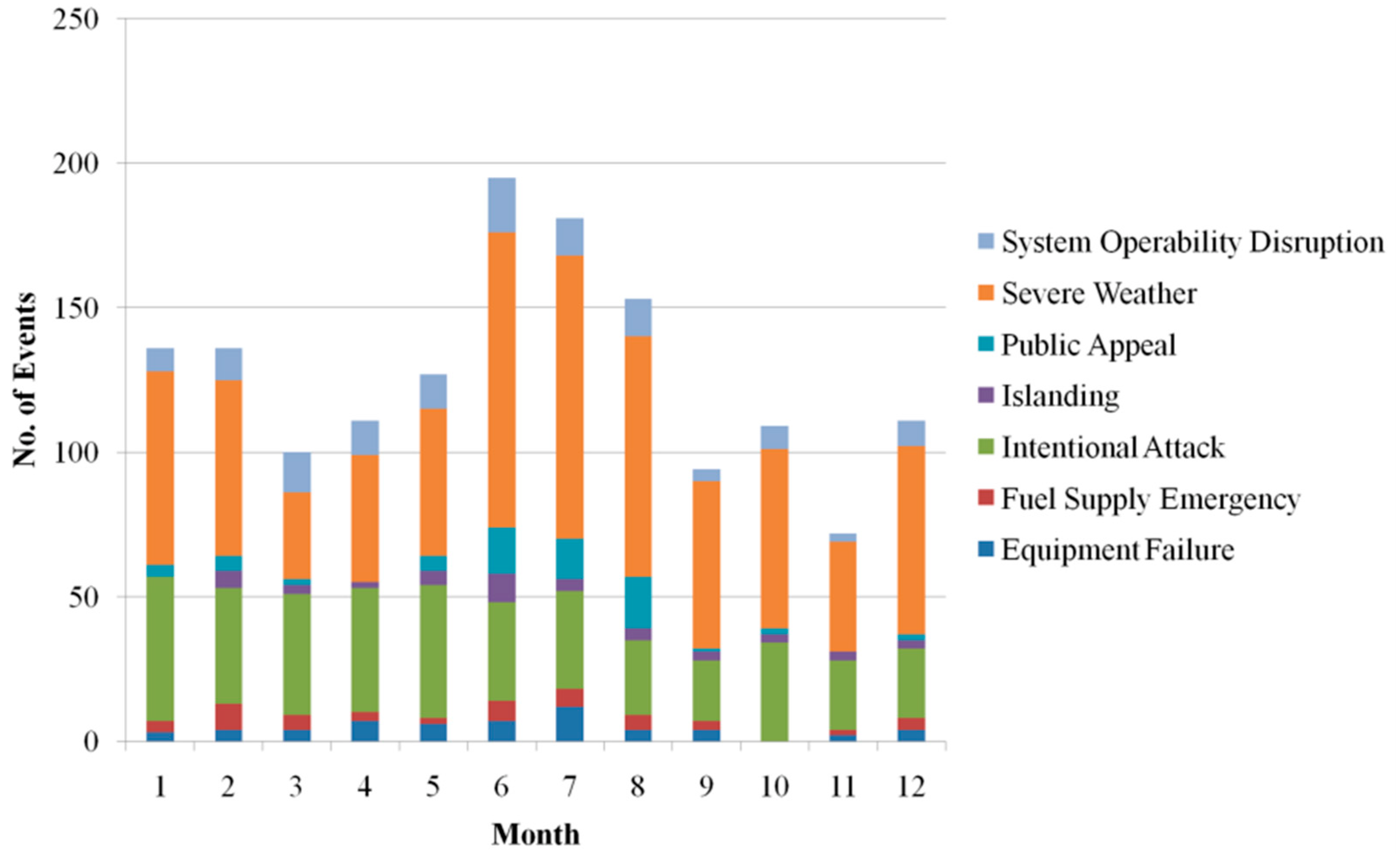
To understand the frequency of such events in relation to different seasons, the month-wise histogram of occurrence of these events is shown in Figure 2, where the histogram shows the frequency of a particular event over the entire period (i.e., 2000–2016). It can be observed that the frequency of severe-weather-related outage events is high during the summer months (i.e., June–August), where 92 events occurred on average per month. In contrast, during the winter season, specifically December–February, 64 events happened on average in a month.

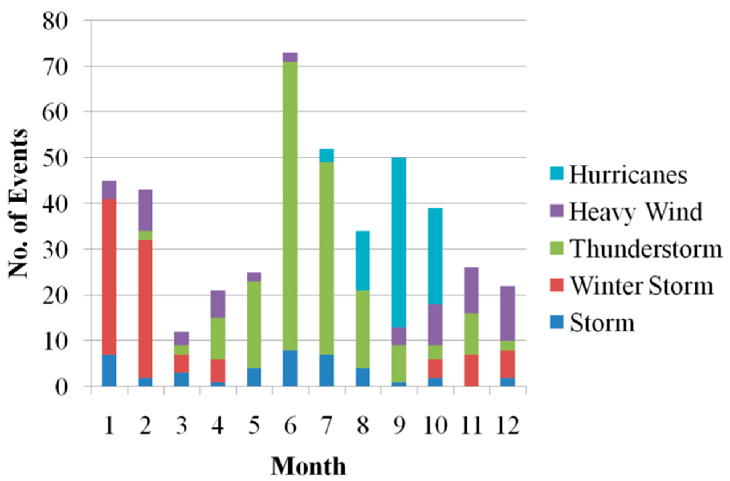
As shown in Figure 1, half of the total number of outage events occurred due to severe-weather-related natural disasters. A statistical analysis of the classes of severe-weather-related natural disasters reveals that 58.2% of the total outage events occurred due to five categories of disasters. The monthly histogram visualization of those types of severe-weather natural disasters is presented in Figure 3. Here, winter storm can be observed as the main cause of power outages during the winter season, while the main cause is thunderstorm for the summer season.

Power outages affect consumers across all sectors, including residential, industrial, and commercial. The electricity cost or the tariff offered to one sector consumer is usually different from the other. The electricity suppliers generate their revenue from the sale, which depends on the consumers’ demand. Whenever a power outage occurs, the supply is cut and so is the sale. Therefore, the power suppliers generate no revenue during the outage. The longer the outage, the larger is the revenue loss. To make an estimate of the revenue loss during an outage event, the sale of an individual consumer sector at the time of the outage event is calculated using Equation (1). The total revenue loss during an outage event is the product of the total sale and the total outage duration, computed using Equation (2). Here, the total sale is the sum of income from all the individual consumer sectors, including residential, commercial, and industrial. The total revenue loss over the sixteen-year period is the sum of all the individual event losses from 2000 to 2016.

$$\mathrm{Total}\mathrm{Sale}\mathrm{per}\mathrm{sector}\left(\mathrm{USD}\mathrm{million}/\min \right)=\frac{\mathrm{Elec}.\mathrm{sale}\left(\mathrm{MWh}\right)\times \mathrm{Elec}.\mathrm{price}\left(\mathrm{cents}/\mathrm{KWh}\right)}{60\times {10}^5}$$

(1)

Total Revenue loss (USD million) = Total Sale (USD million/min) × outage duration (min)

(2)

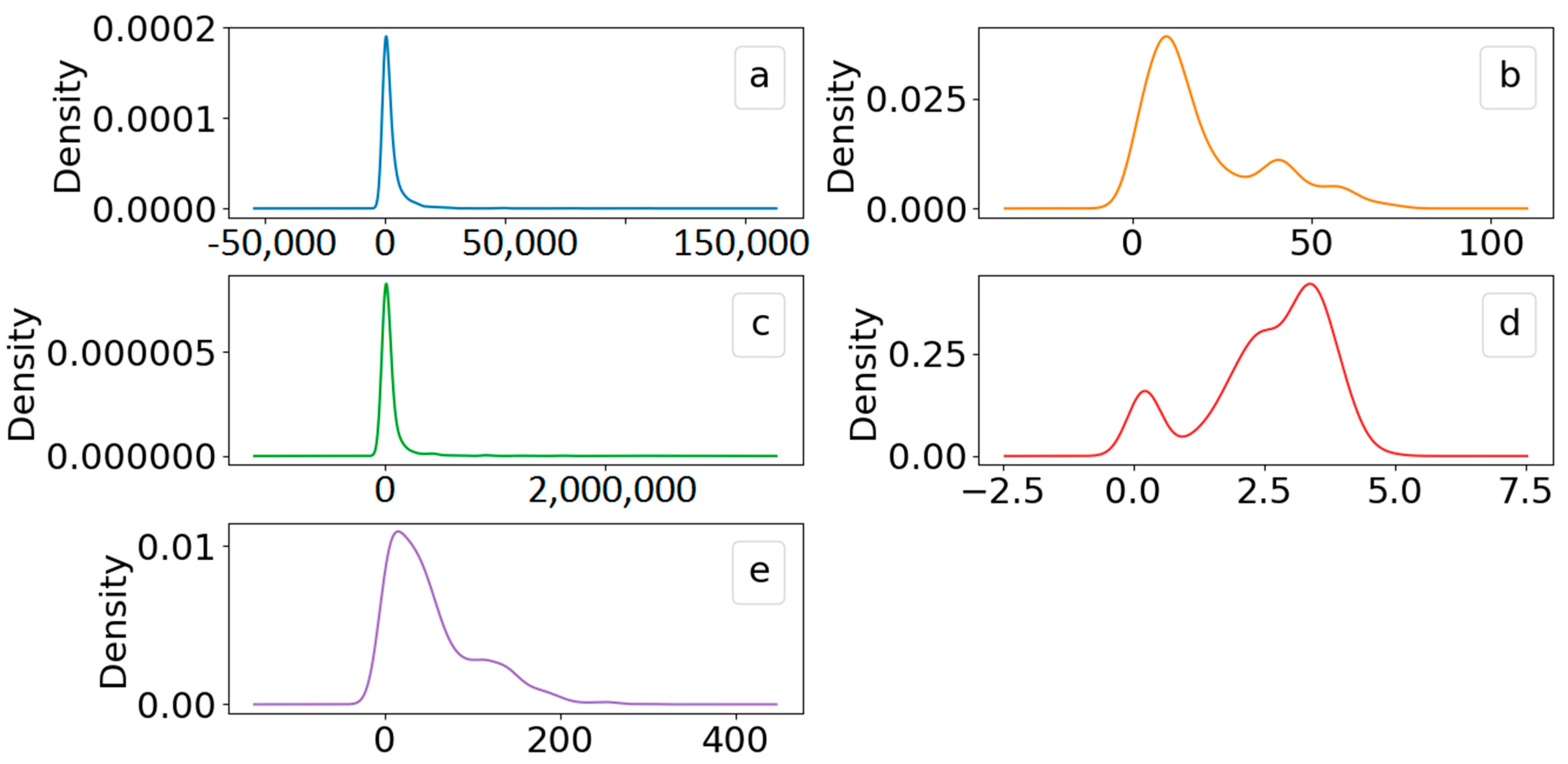
The revenue loss is considered as the output parameter, since the prediction of such loss is performed for the future power outage event in the coming sections of this paper. The unit price for electricity consumption is measured in USD cents (USD 0.01) per KWh, where the unit of consumption is MWh (megawatt hour). From the available data, it was observed that the majority of outage events lasted for a relatively small time period, while fewer events caused prolonged outages. The visualization of observed (actual) outage duration parameter as kernel density distribution reveals this phenomenon, as shown in Figure 4a. It can be observed that the distribution is positively skewed. For improved representation and better visualization, the log-transform version of outage duration is computed and shown in Figure 4b. The log-transformed observations of outage duration are obtained using Equation (3). The density distribution of total sales in USD millions is shown in Figure 4c. It is worth mentioning again that total sale is computed by adding the sale of all individual sectors at the time of occurrence of the power outage event. The density distribution of total revenue loss using transformed outage duration (TLTra) is shown in Figure 4d, while the density distribution of total revenue loss using observed outage duration (TLO) is shown in Figure 4e.

Transformed outage duration = log (observed outage duration + 1.1)

(3)

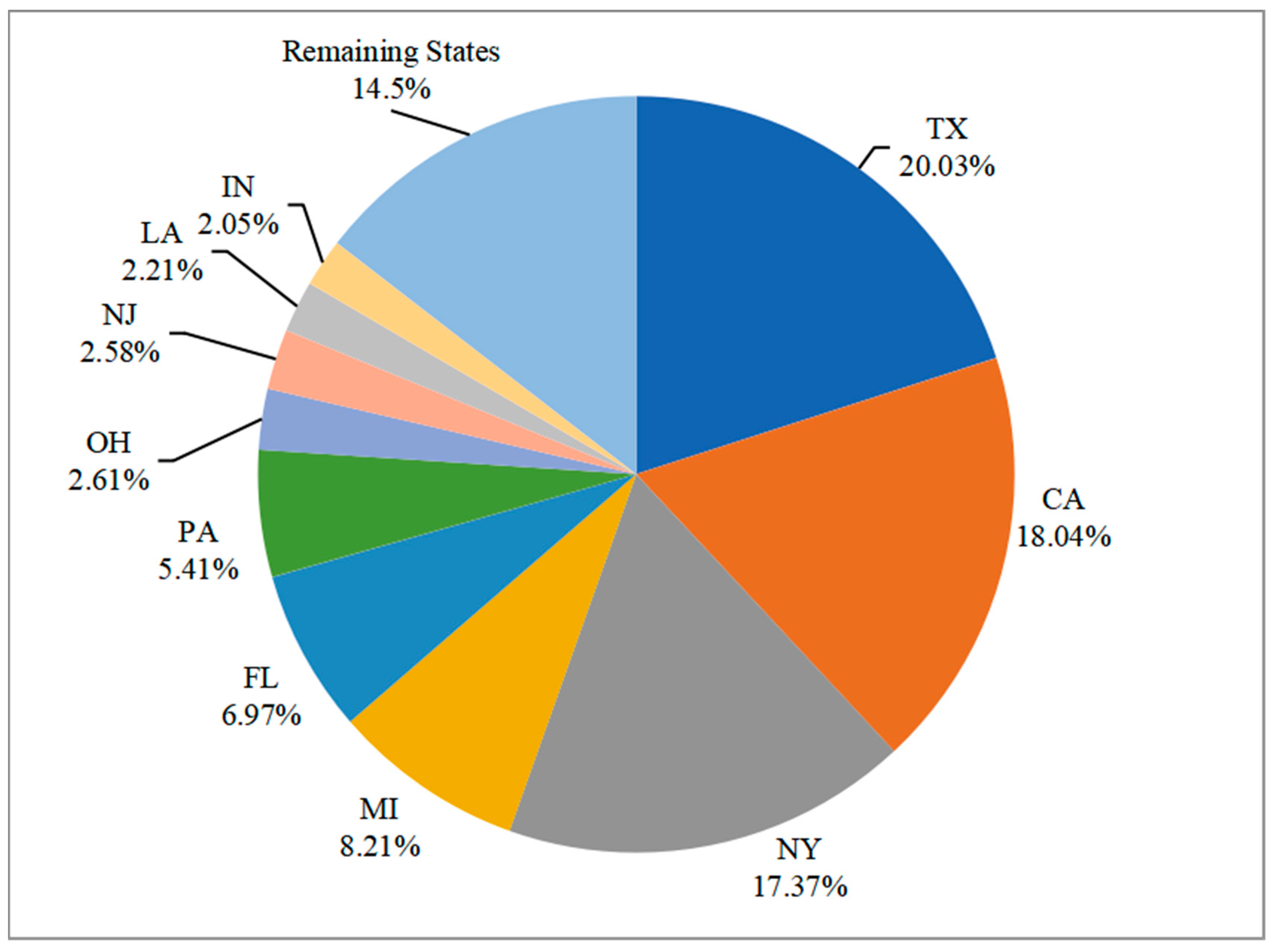
The historical data includes the information of power outage events from 50 States of the U.S. So far in this research, the electricity sale, the revenue generated, and the loss for all the states of the U.S. overall have been computed. Similarly, we will next compute the revenue loss at the individual state level. Figure 5 reveals that 85.4% of the total accumulated loss belongs to 10 states, including Texas (TX), California (CA), New York (NY), Michigan (MI), Florida (FL), Pennsylvania (PA), Ohio (OH), New Jersey (NJ), Louisiana (LA), and Indiana (IN). Interestingly, all those states belong to the North American region. Among them, Texas, California, and New York accumulate more than 55% of the total revenue loss.

The density distribution of the top 10 states’ data, similar to Figure 4, is presented in Figure 6. The similarity between both the figures is evident, since the visualization in Figure 6 projects 85% of the data used for Figure 4.

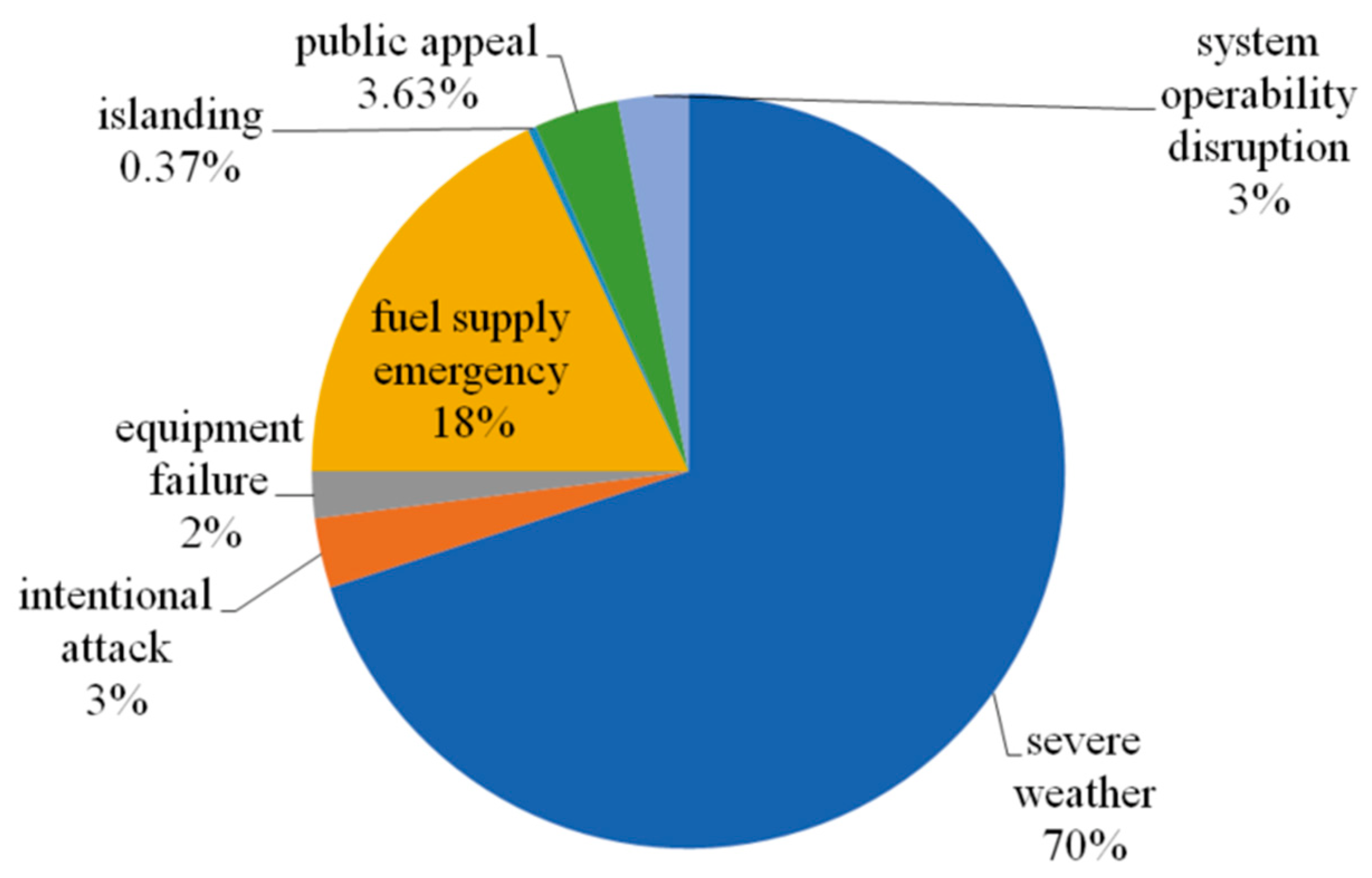
As discussed earlier, there are seven different kinds of events covered in the historical data causing power outage; it is important to see the contribution of each of those events toward the revenue loss. Figure 7 shows the accumulated revenue loss in percentage due to those seven events. It can be seen that severe-weather-related events are responsible for 70% of the total revenue loss. Previously, in Figure 1, it was shown that 50% of outage events happened due to disasters related to severe weather; however, the accumulated revenue loss due to such disasters is even higher (i.e., 70%). This is because of the prolonged outage durations that occur due to natural disasters, in contrast to the other events.

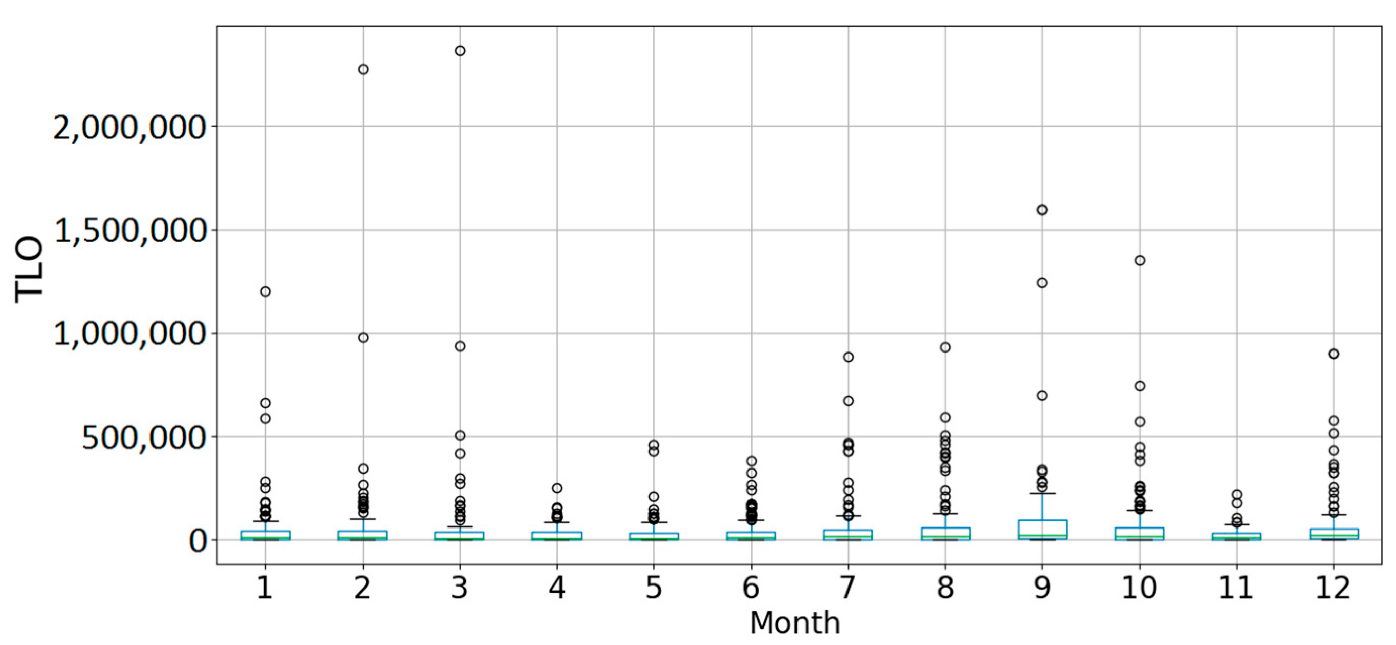
As observed from Figure 2 and Figure 3, the frequency of natural disasters is high during the extreme summer and winter seasons. To see the corresponding impact on revenue loss, a box plot of monthly revenue loss in USD millions is illustrated in Figure 8 for the U.S. overall. The box plot in Figure 8 shows that the revenue loss is higher during June–October as well as December-January compared to the other months. As expected, this is due to the frequent occurrence of severe-weather-related outage events during those periods. Since the box plot also provides insight into the quartile ranges of the data, it can be observed that there are many outliers in the data. Such outliers make the data noisy and lead to high generalization error of the classifier.

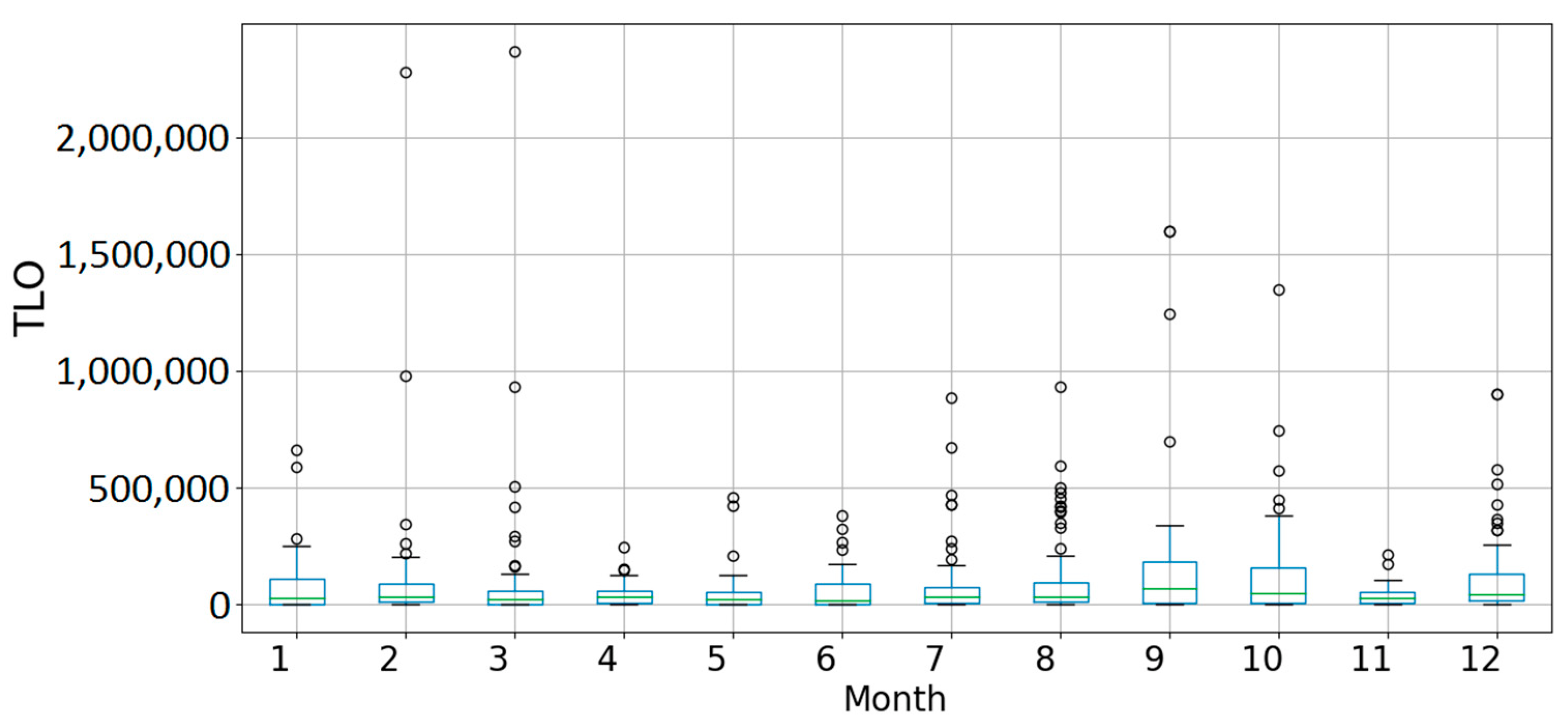
Figure 9 illustrates the monthly dispersion of the revenue loss in USD millions calculated for the top 10 most affected states. A similar pattern to the one in Figure 8 can be observed here as well, since it projects 85% of the total loss.

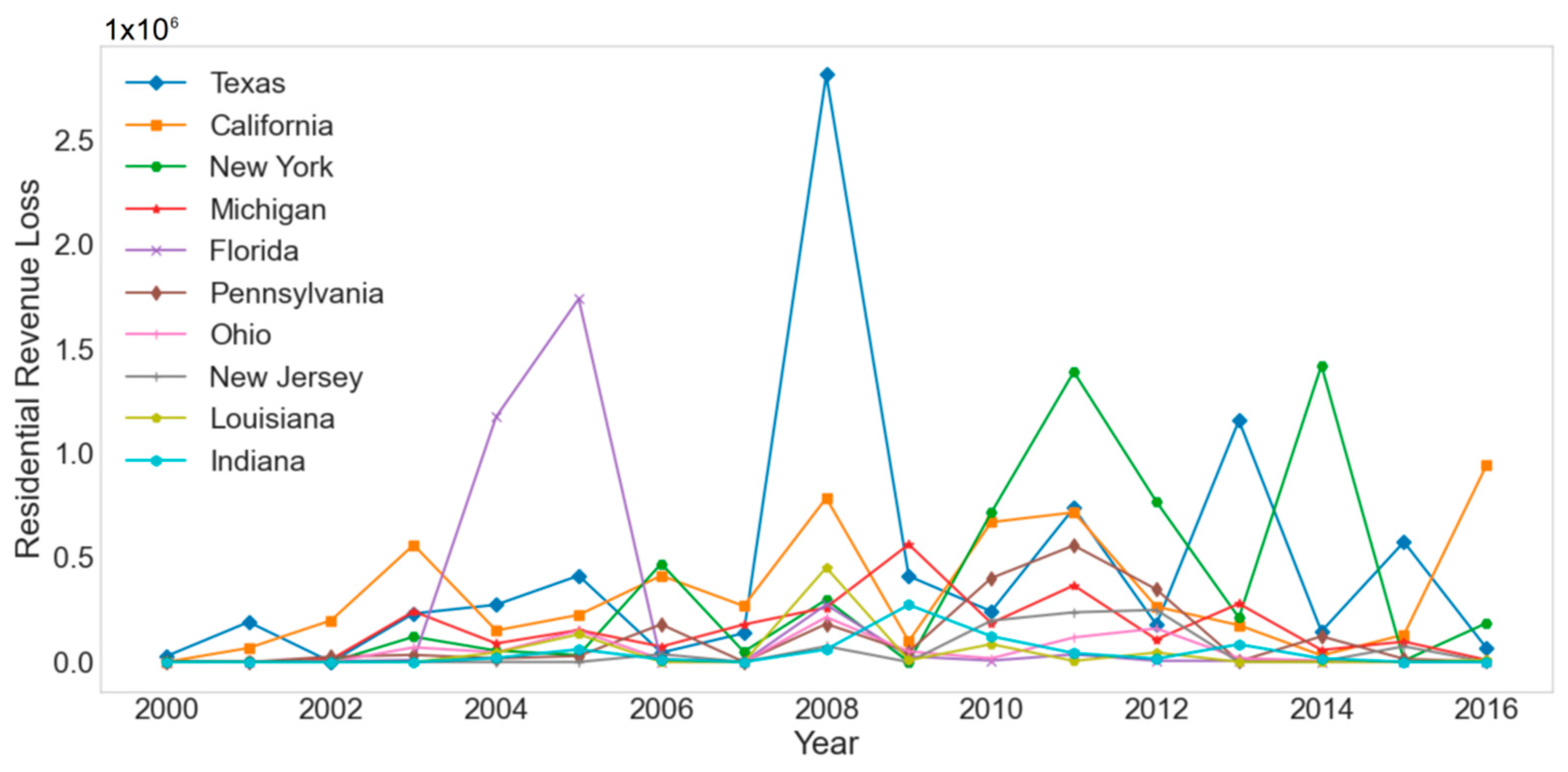
The main source for revenue loss computation is electricity sale and the proposed tariff. This varies among different consumer sectors. For instance, the demand is usually highest in the commercial sector, while the tariff, in contrast, is normally highest for the residential consumers. As established earlier, 85.4% of the total loss happened in the top 10 states; therefore, we visualize the annual revenue loss for those individual states. Figure 10 shows the revenue loss for each of the top ten states in the residential sector over the period from January 2000 to July 2016. It is observable that New York, California, and Texas have seen larger losses over the entire period overall. It is also observable that the revenue loss is highest for the year 2008, specifically in Texas. This is due to the occurrence of prolonged outages in the months of July and September under severe weather conditions, particularly due to hurricanes. The largest outage duration observed spanned over twenty days in September 2008.

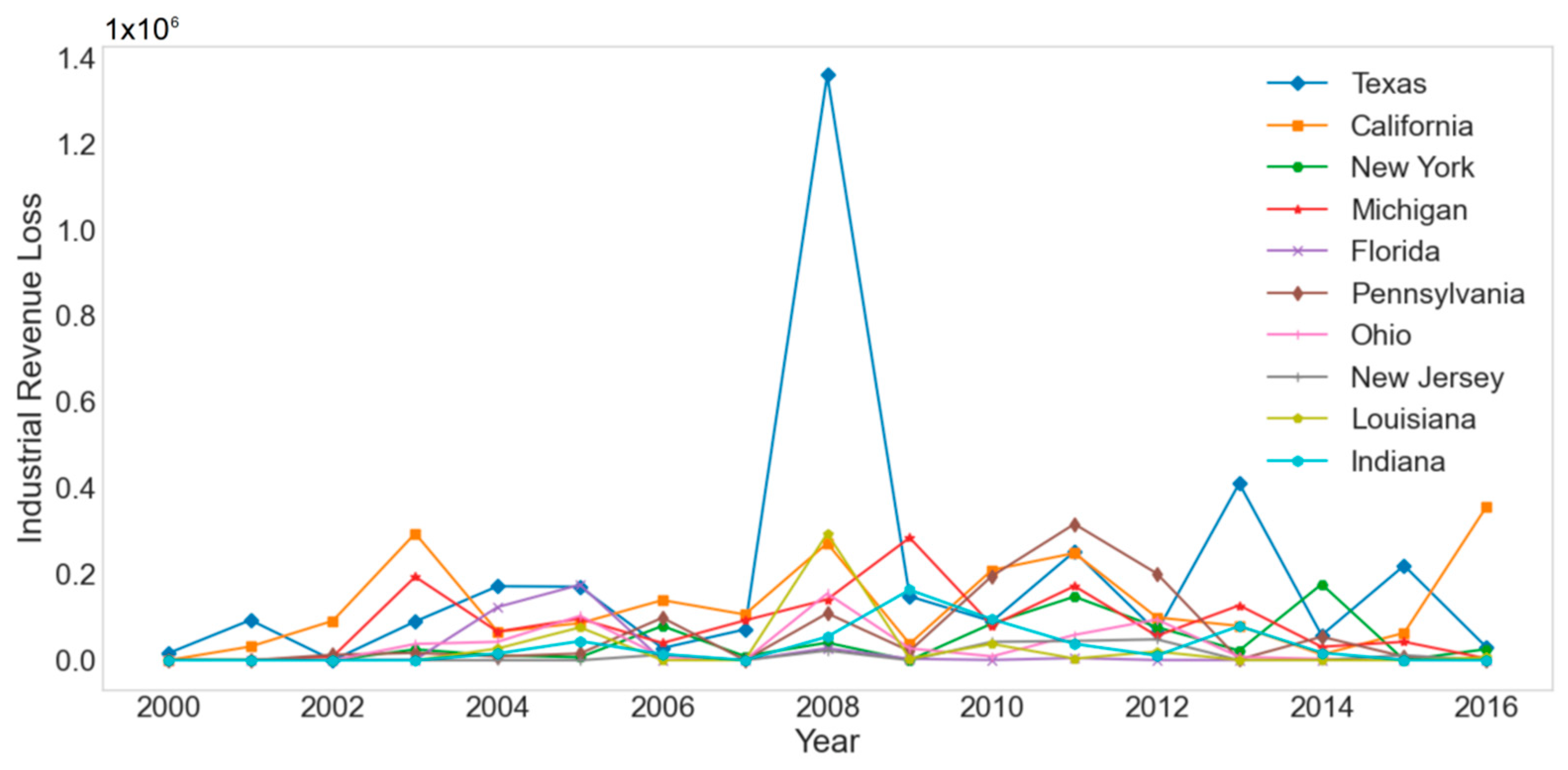
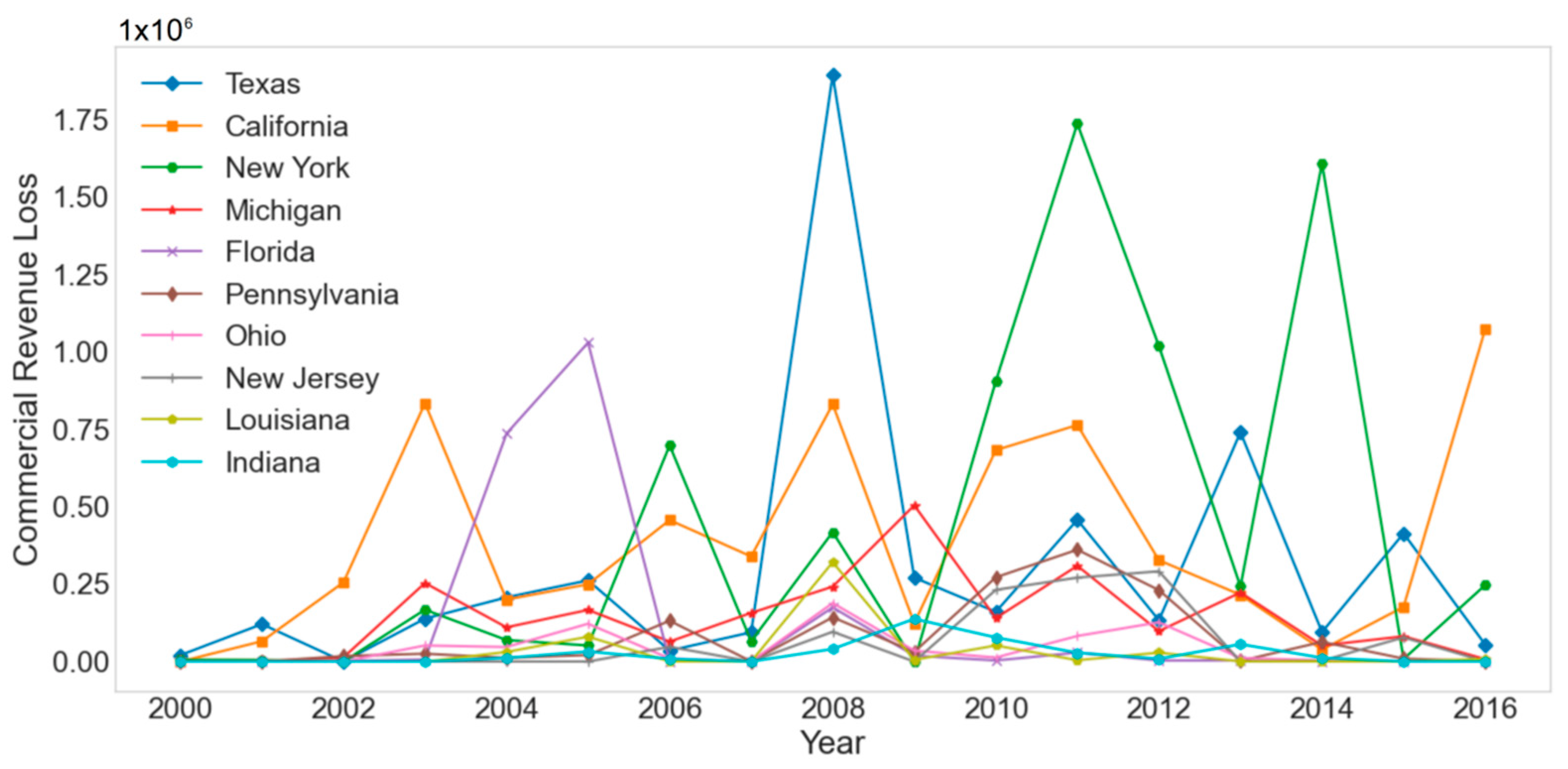
Similarly, the revenue losses can be seen in Figure 11 and Figure 12 for the industrial and commercial sectors, respectively. A similar trend can be observed with respect to the individual states. A comparison of the sectors shows that the revenue loss is highest in the commercial sector. As mentioned earlier, the commercial sector is often more demanding than other sectors; the demand of the commercial sector is almost 160% that of the residential sector. However, it is worth mentioning that, according to the data, the price of the commercial sector electricity is lower, almost 70% that of the price of the residential sector on average. The trend of high commercial revenue loss is almost consistent in all the individual states; however, it is comparatively higher in the states of Texas, California, and New York. The high demand and the tariff are the reasons. Now, excluding the commercial sector, the loss is comparatively higher for the residential sector than the industrial sector. This is because of the relatively higher electricity rate, almost twice comparatively, as well as the higher demand in general.

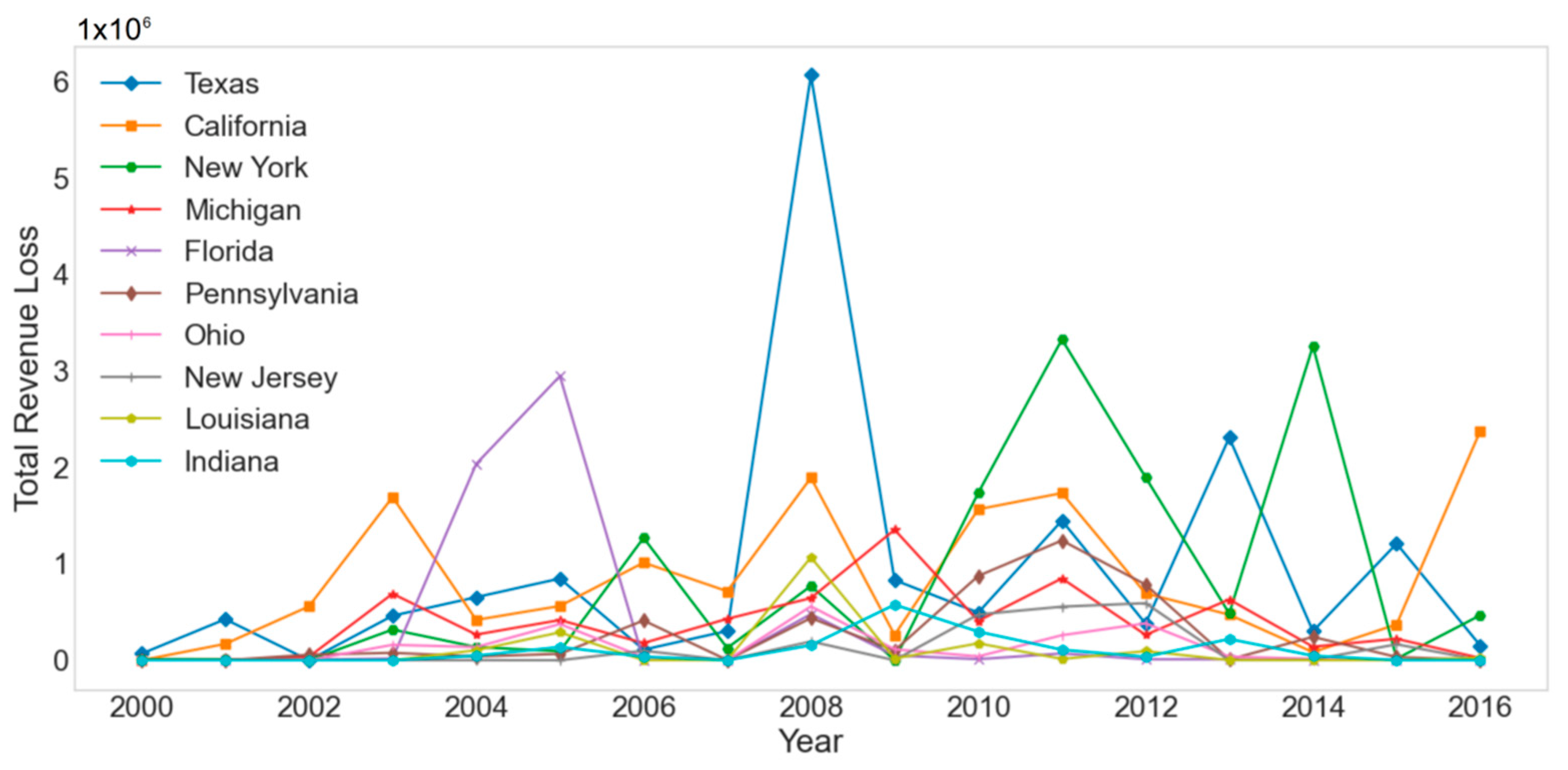
Figure 13 shows the yearly combined revenue loss of the three sectors over the total 17-year duration. The total revenue loss is the sum of the losses computed at the level of the individual sectors.

Finally, we present the statistical analysis for revenue loss in the

Table 2. Statistical analysis of the total revenue loss for top 10 states and the U.S. overall.

Revenue Loss (Million USD)		Statistical Parameters
		Mean	Median	Std. Dev.	Min	Max	IQR
U.S. Over all	TLO	55,190	12,455	155,065	0	2,366,544	45,972
	TLTra	125	91	118	0.04	685	147
Top10 States	TLO	93,718	33,494	204,404	0	2,366,544	86,451
	TLTra	202	180	119	0.04	685	172

TLO: total loss calculated based on observed outage duration. TLTra: total loss calculated based on transformed outage duration.

, calculated using both observed and transformed outage duration. It is observable that the statistics for the top 10 states of the U.S. have greater values (for instance, the mean, the median, and the IQR). The reason is obvious; the majority of instances for the top 10 states belong to prolonged outage events, where the duration of outage spanned from days to weeks. In comparison, for the overall U.S. level, many short-duration outages exist along with the prolonged ones, leaving the mean outage duration smaller. The outage events that lasted for a few seconds (less than a minute) were rounded up and recorded as zero minutes. That explains why we added a constant in log transformation when computing the transformed outage duration. It is worth mentioning that when calculating the financial loss associated with transformed outage duration, the outage durations are initially log-transformed (using Equation (3)) and then multiplied with the price (using Equation (2)) to obtain the transformed loss.

4. Methodology

So far, a detailed exploratory data analysis has been carried out by observing the events responsible for power outages, the major events primarily responsible for power outages (weather-related natural disasters), the revenue loss both for observed (actual) outage duration and the transformed outage duration, the monthly distribution analysis for events, and the losses. The aim is to perform a prediction of revenue losses in the case of power outages due to any kind of event that has been observed. Therefore, the revenue loss is selected as the response (or output) variable, to be predicted using machine learning techniques. There are a number of machine learning algorithms that have been used for prediction, such as linear regression, support vector machines (SVM) [30], artificial neural networks (ANN) [31], and decision trees [32]. The selection of the appropriate technique is important, since each has its associated pros and cons. The SVM is a popular machine learning technique, also called the large margin classifier. It can fit both linear and non-linear models to the data. However, it is largely used for classification purposes rather than regression problems, as in the current scenario. The decision tree is a low-bias, high-variance technique and therefore causes over-fitting. Moreover, it is sensitive to noise and outliers, which leads to large generalization errors.

The nature and size of the data set plays an important role. The data used in this research is multidimensional and diverse, and therefore the presence of noise and outliers is likely, as can be observed in the box plots in Figure 8 and Figure 9. Keeping in view the nature of the data and the problem-specific machine learning algorithms, the artificial neural network (ANN) and the random forest algorithms are selected for the prediction and results evaluation. The ANN is a state-of-the-art technique that has been used in multidisciplinary research for regression as well as classification purposes [33,34,35]. The random forest is an ensemble tree-based method. A brief description of these methods, along with definitions of illustrative evaluation methods, is included in the following subsections.

4.1. Artificial Neural Network Model

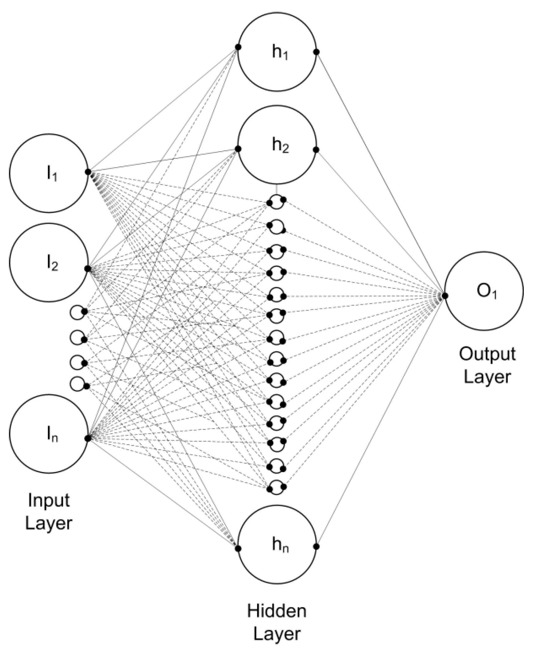
An artificial neural network (ANN) consists of a layered structure with interconnected nodes, called neurons. It is a data-driven algorithm whose working mechanism is inspired by the biological nervous system. The data is fed as input at the first layer of the ANN, and the output layer produces a prediction of the network. A multilayer ANN may have one or more hidden layers (which include all the layers other than the input and the output layer). Generally, one hidden layer is sufficient to map the input–output relationship; however, it may require more layers to accommodate highly complex data. The prediction error is iteratively reduced using the back-propagation algorithm, used for training of the neural network [36]. Once the network is trained by achieving the minimum training error, the network is evaluated using the unseen data. A sample model of an artificial neural network with an input layer, a hidden layer, and an output layer is shown in Figure 14. The first layer is the input layer, where the features are applied to the neural network. Therefore, I₁ represents the first input feature, h₁ represents the first hidden unit, and O₁ represents the first output unit. Since there is only one output in our case (i.e., the revenue loss), only one output is shown. The n is an arbitrary number that represents the total number of input features, and the same is used to represent the total number of hidden units in the hidden layer. The actual number of input and output units of the estimated network will be discussed in the coming Results and Discussion section.

4.2. Random Forest Model

Brieman originally developed the random forest (RF) model [37]. It is a tree-based ensemble algorithm that can comprehend the nonlinear nature of the data and is robust to outliers and the noise. It is a non-parametric technique; therefore, it does not reflect any particular distribution and performs efficiently for heterogeneous data, making it suitable for problems with diverse data. It is easy to implement, without any need for fine tuning, and produces reasonably good results. The procedure to develop a random forest algorithm is as follows [37]:

• Select N re-sampled batches of data as training set and keep the remaining data for validation.
• Choose m variables to split and fit the regression tree.
• Choose the optimal splitting value and let the tree grow.
• Compute the prediction error by using residual data.
• Repeat the steps 1–4 K times to establish K number of trees.

Random forest apprehends the broad structure of the data and has sensitivity to outliers, which is the high-variance scenario. Since each individual regression tree is fit on random subsets of data, and the split of the tree is random as well; therefore, taking averages of the estimates of all the trees overcomes the high-variance impact and improves the accuracy. These features make it a perfect algorithm to fit compound and noisy data.

4.3. Partial Dependance Plots

Partial dependence plots provide insight into the influence of an individual feature, such as economic indicators, land area, population, time of the event, and so on, on the response variable (revenue loss). In non-parametric models, PDPs reveal the impact of a single feature on the output considering all the other factors to be constant. It is an effective way to show the bordering effect on the output parameter by keeping all the features unchanged except one [38]. A PDP can be computed as follows:

$$Y_s(X_s)=\frac{1}{K}{\displaystyle \sum _{i=1}^{K}Y(X_s,x_{iR})}$$

(4)

where Y_s is the output variable, X_s represents the covariate for which the PDP to be estimated, and x_iR are all the covariates except X_s.

4.4. Quantile–Quantile (QQ) Plot

A quantile–quantile (QQ) plot is a graphical way to compare two probability distributions by plotting their quantiles against each other. When the two distributions are identical, the QQ plots follow a 45° line (i.e., y = x). If the line is relatively flatter, the distribution plotted on the horizontal axis is more dispersed than the one on the vertical axis. Conversely, the relatively steeper line indicates a higher dispersion of the distribution on the vertical axis than that on the horizontal axis.

4.5. Final Feature Selection for Loss Estimation

Since the data in this study is multivariate, it is important to look at the multi-collinearity. It may avert the impact of input features on the output variable, which needs to be addressed. To reduce the multi-collinearity in the data, only the features with a variance inflation factor (VIF) less than 4 are short-listed [39]. The VIF is the ratio of the variance in a model with multiple terms to the variance of the model with a single term. It shows how the variance of an estimated regression coefficient is increased due to collinearity. The VIF is computed to select the final features to be used for the prediction of revenue loss, both for TLO and TLTra. The finally selected features are summarized in

Table 3. Final set of features selected for prediction of revenue loss.

Feature	For Total Loss (Observed Outage Duration)	For Total Loss (Transformed Outage Duration)
Year	×	×
Month	×	×
Anomly_level	×	-
Demand_loss_MW	×	-
Customers_affected	×	-
Industrial_price	×	-
Residential_sales	×	×
PCT_residential_electricity_consumption	-	×
PCT_commercial_customers	×	×
PCT_Industrial_customers	×	×
PC_real_GSP_USA	×	-
PC_real_GSP_change	×	×
Utility_contribution	×	×
PC_real_GSP_REL	×	×
PCT_land_area_urban	×	×
PCT_land_area_state.level	×	×
PCT_inland_water_area_state.level	×	×
Postal_code	×	×
PCT_population_urban_cluster	-	×
Severe_weather_catgory	×	×
Climate_region	×	×

× = Yes, - = No.

separately for TLO and TLTra.

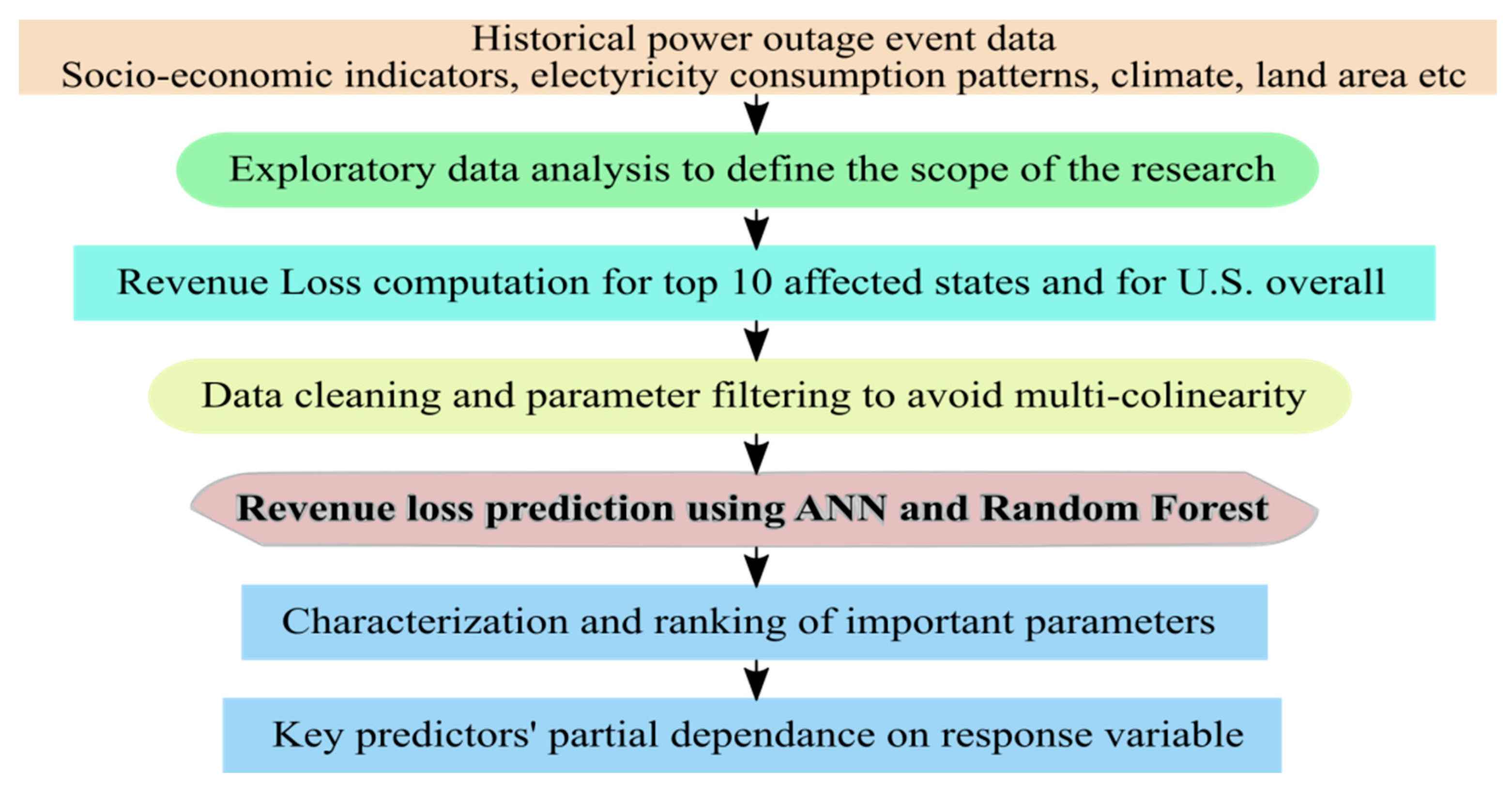
The exploratory data analysis in Section 2 revealed that more than 85% of the financial loss is borne by only 10 states of the U.S. Therefore, from this point on, further analysis and results evaluation are carried out using the data of those 10 states. The final features presented in Table 3 are also estimated using the data of the top 10 most affected states. The overall workflow of this study is expressed in the block diagram shown in Figure 15.

5. Results and Discussion

Since the prediction of the revenue loss is a regression problem in nature, for results evaluation, several error metrics are considered, such as mean absolute error (MAE), mean absolute percentage error (MAPE), root mean square error (RMSE), and accuracy. Since the target and the predicted value are both real numbers, the mean absolute error provides the average difference between the two. MAPE provides a better insight about the prediction results in terms of percentage error. The RMSE is another widely used error metric to compute the error between two real values. These error metrics are mathematically expressed as follows:

$$MAE=\frac{{\displaystyle \sum _{i=1}^n\left|y_i-p_i\right|}}{n}$$

(5)

$$MAPE=\frac{1}{n}{\displaystyle \sum _{i=1}^n\frac{\left|y_i-p_i\right|}{y_i}}$$

(6)

$$RMSE=\sqrt{\frac{{\displaystyle \sum _{i=1}^n{\left(y_i-p_i\right)}^2}}{n}}$$

(7)

where y_i is the actual value, p_i the predicted value, and n the total number of observations. The accuracy is computed as 1-MAPE.

It is worth mentioning the hardware and software resources used for this study. The experiment was performed on an Intel Core i3 2.2 GHz processor machine with 4 GB RAM. On the Windows 10 operating system, a Python programming environment was used with the Keras library for implementing machine learning algorithms. The execution time for training and testing data for neural network was recorded as 2.12 s and 1.04 s, respectively. For random forest, the execution time was recorded as 1.53 s and 0.67 s for training and testing data, respectively.

5.1. Neural Network Model Prediction

For the neural network model, architecture with a single hidden neuron is selected. For the training of the network, the data is randomized and split into 70, 15, and 15 percent for the purpose of training, validation, and testing, respectively. The network is trained using the training set and optimized using the validation set, while mean square error is observed for network optimization. The network was optimized, ending up with 22 hidden neurons to achieve minimum validation accuracy. The learning rate was set as 0.001. As mentioned earlier, since the top 10 identified states are considered, the total data is the combination of the observational outage data of the top 10 identified states, independent of state affiliation. The objective is to predict the revenue loss independent of the location of the event.

The results using the neural network model are presented in

Table 4. Final revenue loss prediction results of machine learning algorithms.

Predicted Revenue Loss per Event (USD Million)
		with Observed Outage Duration	with Transformed Outage Duration
Artificial Neural Network Model	MAE	23,012.7	19.6
	MAPE	24.8	45.3
	RMSE	29,173	26.9
	Accuracy	75.2	54.7
	R2	0.68	0.56
Random Forest Model	MAE	19,063.9	16.2
	MAPE	20.2	38.2
	RMSE	22,356	18.5
	Accuracy	79.8	61.8
	R2	0.76	0.68

for both the observed outage-duration-based loss and the transformed outage-duration-based loss. It can be observed that the MAE for transformed financial loss is much smaller than the observed loss. This is because of the values used at the logarithmic scale. However, to calculate the accuracy of the predicted transformed loss, its inverse-log is taken and compared with the actual loss. In other words, the target value for revenue loss is not changed at all. Prediction using log-transformed values is performed, and the result is converted back by taking its inverse log. In this way, both values are compared, and the error is calculated. The accuracy in the case of actual (untransformed) loss prediction is higher, with a statistically larger error. This is because of scale conversion. The MAPE reflects the results on a similar scale, and it can be observed that this error is almost half in the case of observed revenue loss. The higher value of R²-square also confirms the better prediction results in the case of observed revenue loss.

5.2. Random Forest Model Prediction

For the random forest model, the data is split into training and test sets as 75% and 25%, respectively. During the training, the optimum number of estimators was found to be 200. The prediction results of the random forest model are presented in Table 4. In the context of observed versus transformed, we find in the results a similar pattern as that recorded using the ANN. The results with observed loss are better than those with transformed loss (i.e., the accuracy is 18% higher), and the MAPE is almost half. As a comparison between the models, the random forest produced better prediction results than ANN, achieving lower error and higher accuracy. The reason is its better fit for multi-dimensional, nonlinear, and noisy data with outliers.

5.3. Identification of Important Features

The results in Table 4 revealed that higher prediction accuracy can be achieved using original observed outage duration. Based on this, the final feature set for the TLO from Table 3 is considered for further feature-level analysis. Among those features, the most important ones are identified using the random forest model, since it can be utilized for feature importance ranking. 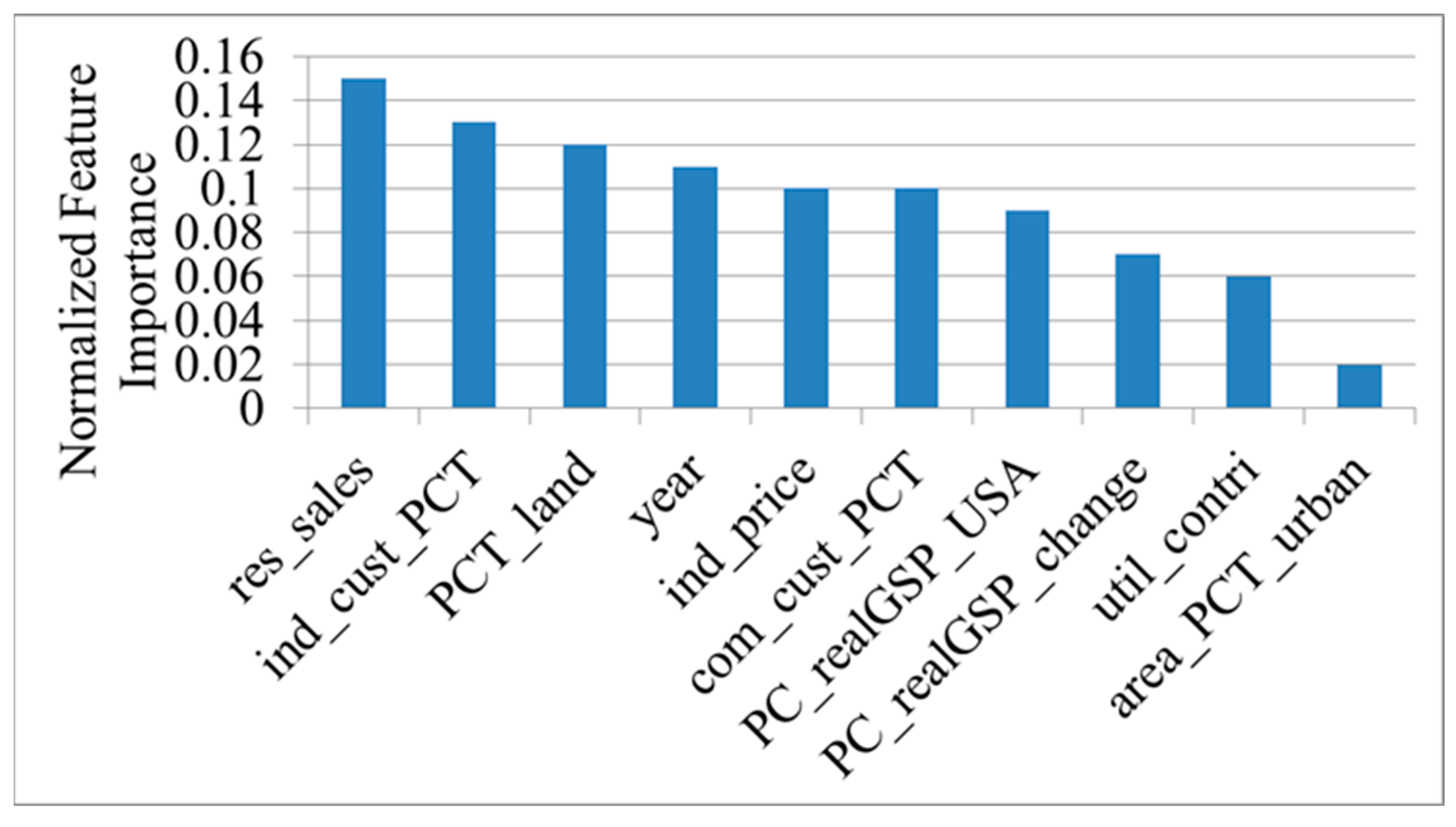Important feature ranking has been carried out in [37], where key features were identified for individual state analysis. The outage duration parameter in this paper is used for calculating the revenue loss; therefore, it has not been considered as an input feature for the revenue loss prediction. Figure 16 shows the important features along with their normalized importance for prediction of revenue loss using observed outage duration. The electricity sale of the residential sector is identified as the most important feature for prediction of revenue loss, followed by percentage of industrial customers and percentage of land area, respectively, as the second and third features.

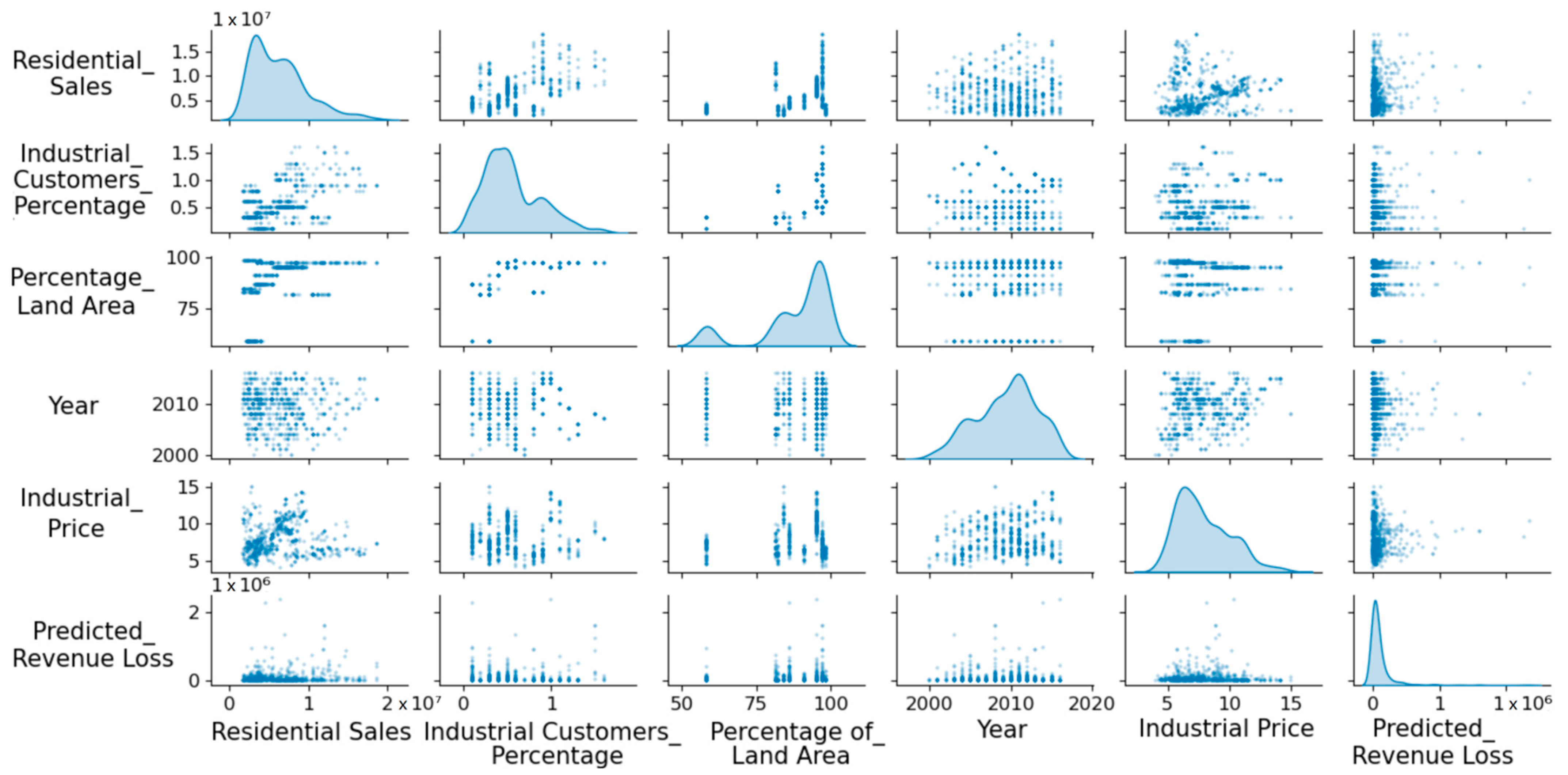
Figure 17 shows the performance analysis graph where the relationship between the top five important features and the response variable is plotted. The off-diagonal plots from left to right show the density distribution of individual features. The bottom row of Figure 17 shows the correlation between the individual feature variable and the response variable (revenue loss). It can be observed that there is almost no correlation between the loss and the individual feature variables. The rest of the plots illustrate the inter-feature correlations. It can be observed from these plots that the majority of the features are uncorrelated with each other, with a couple of exceptions. For instance, the correlation of the residential sales variable with the rest of the variables can be observed in the scatter plots in the first column of Figure 17. The residential sales variable has a positive correlation with the industrial customer percentage variable and the percentage land area variable. Similarly, a minor negative correlation can be observed between residential sales and the year variable.

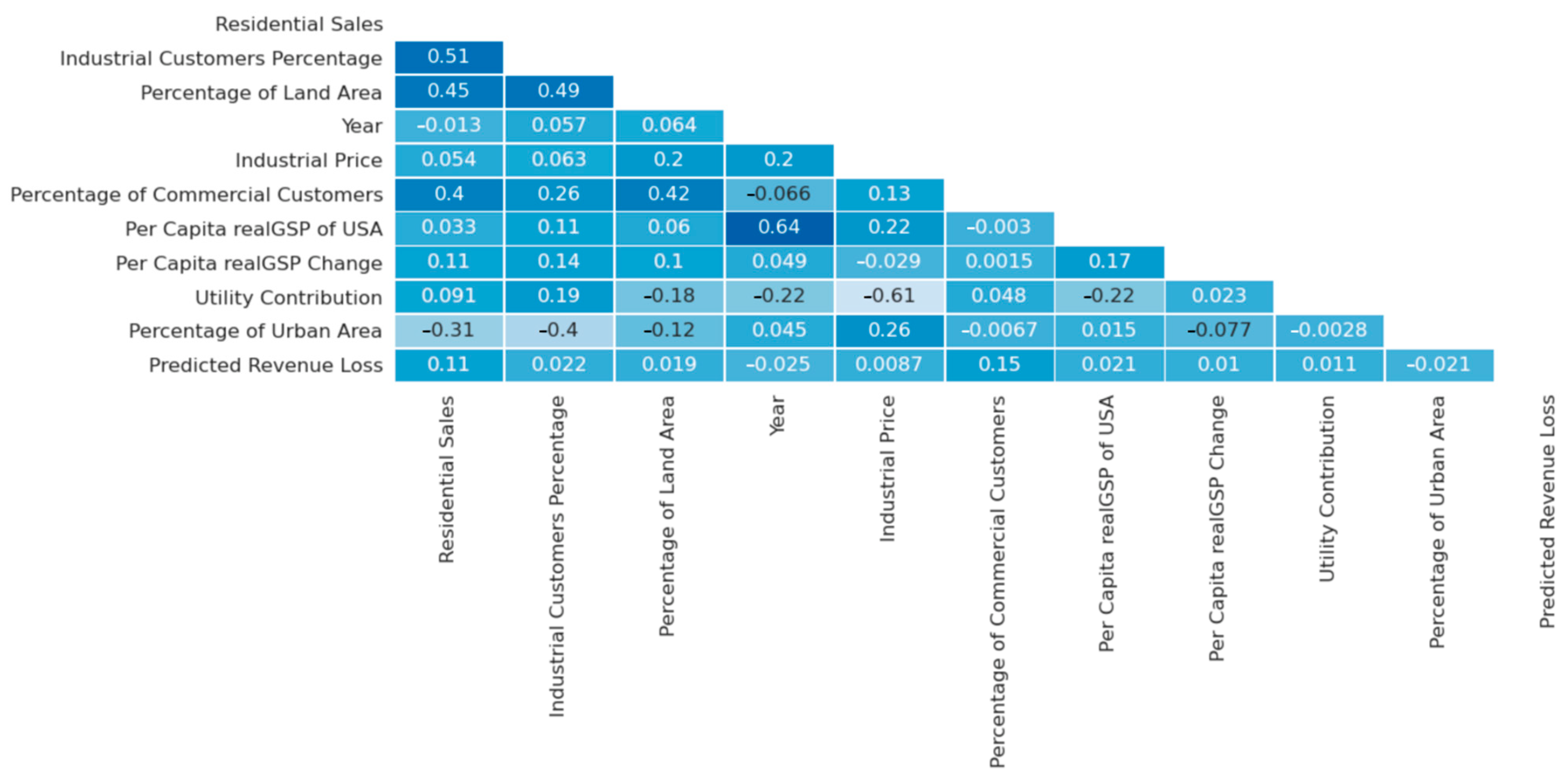
Figure 18 presents the inter-feature Pearson correlation coefficient for the top 10 important feature variables along with the heat map. A higher magnitude of the Pearson correlation index shows a stronger linear relationship between the features, while a negative value represents the inverse relationship. The bottom row of Figure 18 shows the correlation index between individual feature and the predicted revenue loss. The rest of the observations correspond to inter-feature correlation coefficients. A large positive value represents the high positive correlation between the feature variables. For instance, the residential sales variable has a moderate positive correlation with the industrial customers’ percentage, percentage of land area, and percentage of commercial customers variables (see the first column of Figure 18). Similarly, a negative correlation exists between industrial price and utility contribution, with a correlation coefficient of −0.61.

5.4. Partial Dependency Plots

The PDP provides an insight about the effects of individual features on the response variable. In each plot, the range of a feature value influencing the response variable is represented on the horizontal axis. The vertical axis represents the predicted revenue loss in USD millions. For the sake of illustration of partial dependence, we shall discuss the PDPs of the three most important feature variables.

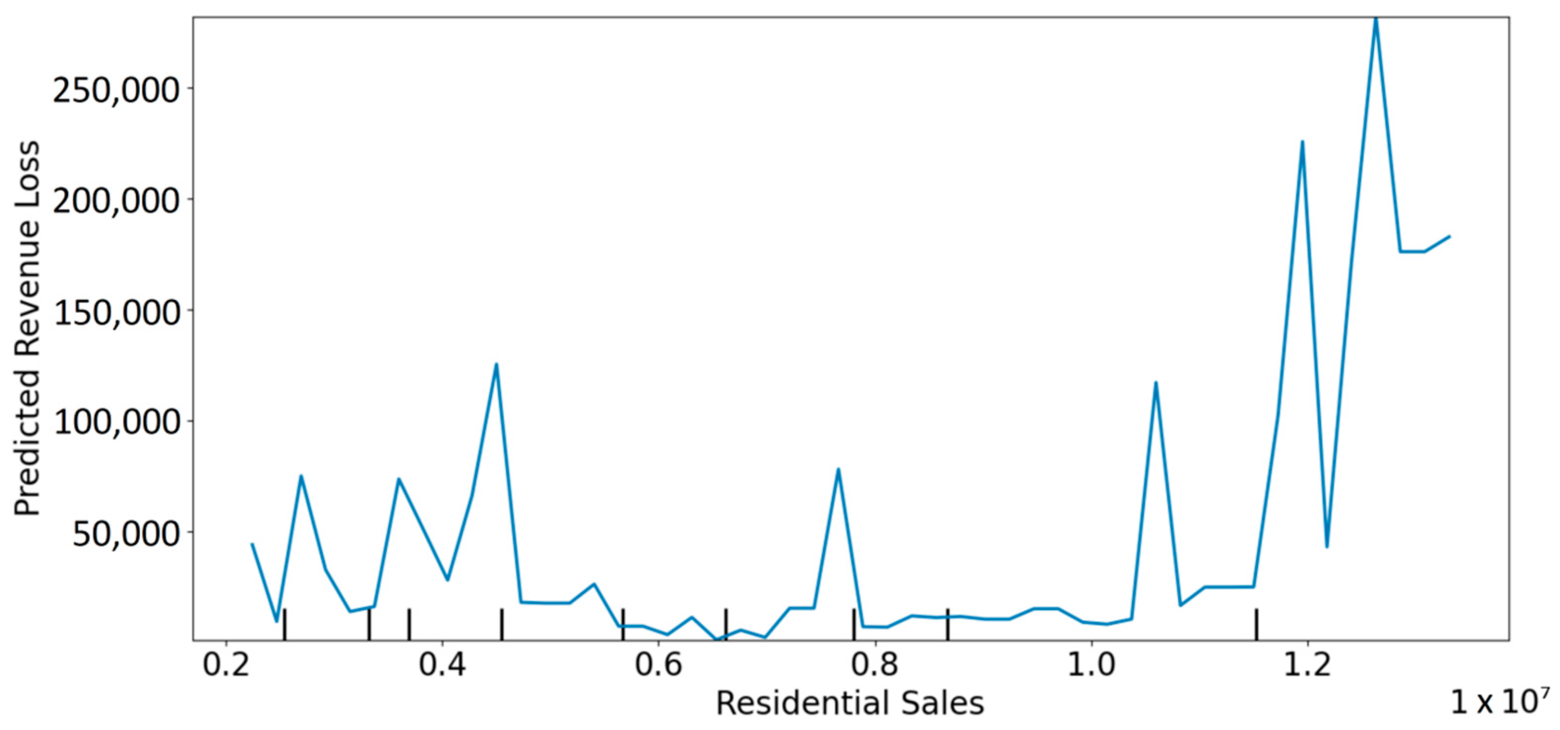
The PDP shown in Figure 19 illustrates the influence of the residential sector electricity sales parameter on the predicted revenue loss. Many peaks of predicted revenue loss can be observed against the residential sales. The effect is generally low in the mid-range of sales, except at 0.75. With a further increase in sales, the predicted revenue loss keeps increasing. In general, there are a few observations of residential sales where the classifier predicts high revenue loss. Other than those, the predicted loss is generally low and constant. The normalized feature importance of residential sales is 0.15; therefore, we noted the effect of residential sales on predicted loss to be less correlated.

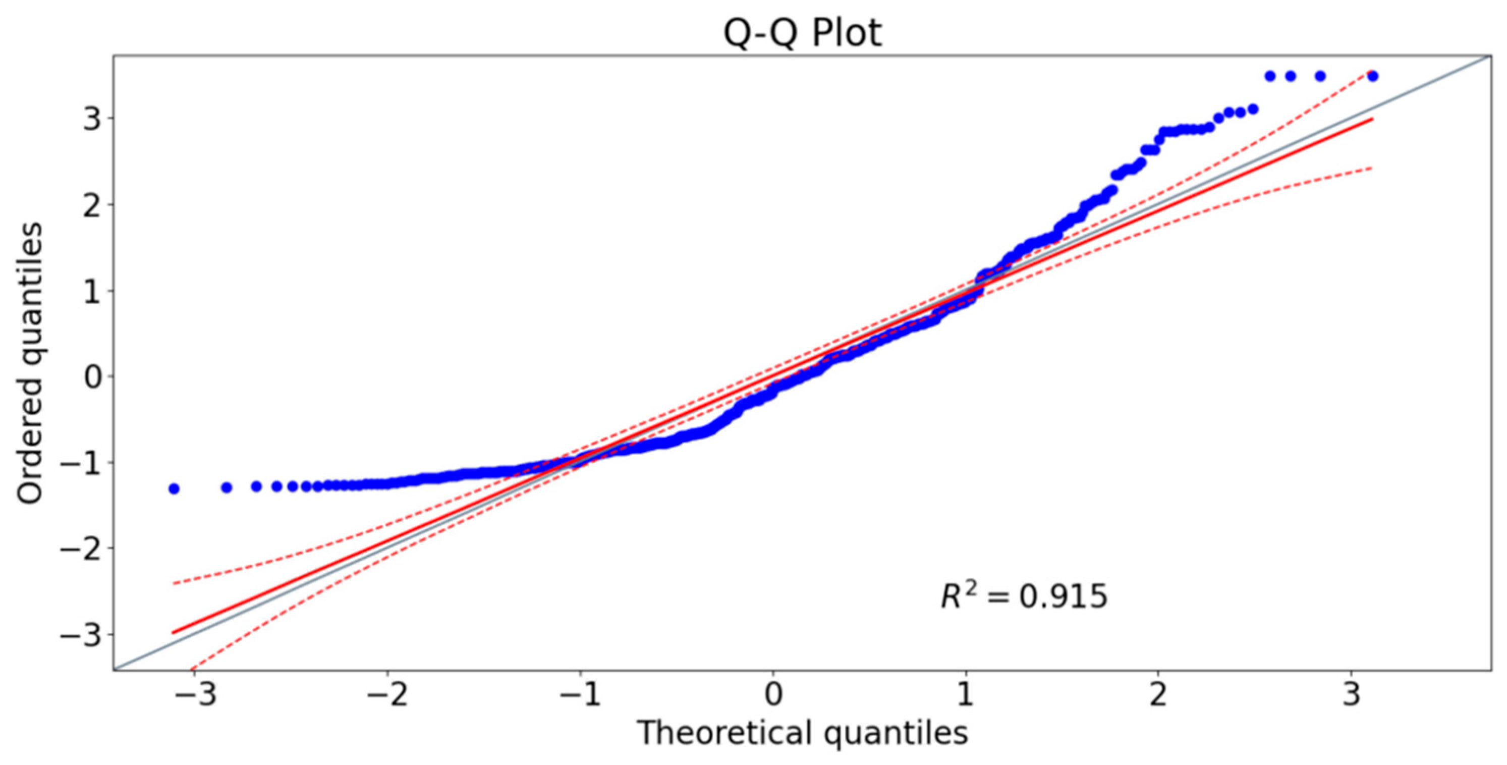
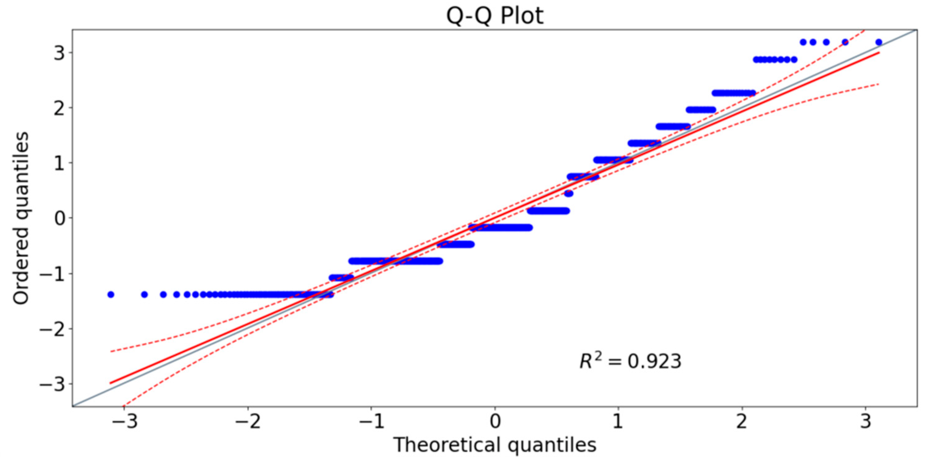
Figure 20 shows the QQ plot between residential sales and revenue loss. The red dashed lines show the 95% confidence interval range. The points forming the S-shape in the plot indicate the dispersion in the probability distribution of both variables. It also suggests that the model may not efficiently capture the variance in the data.

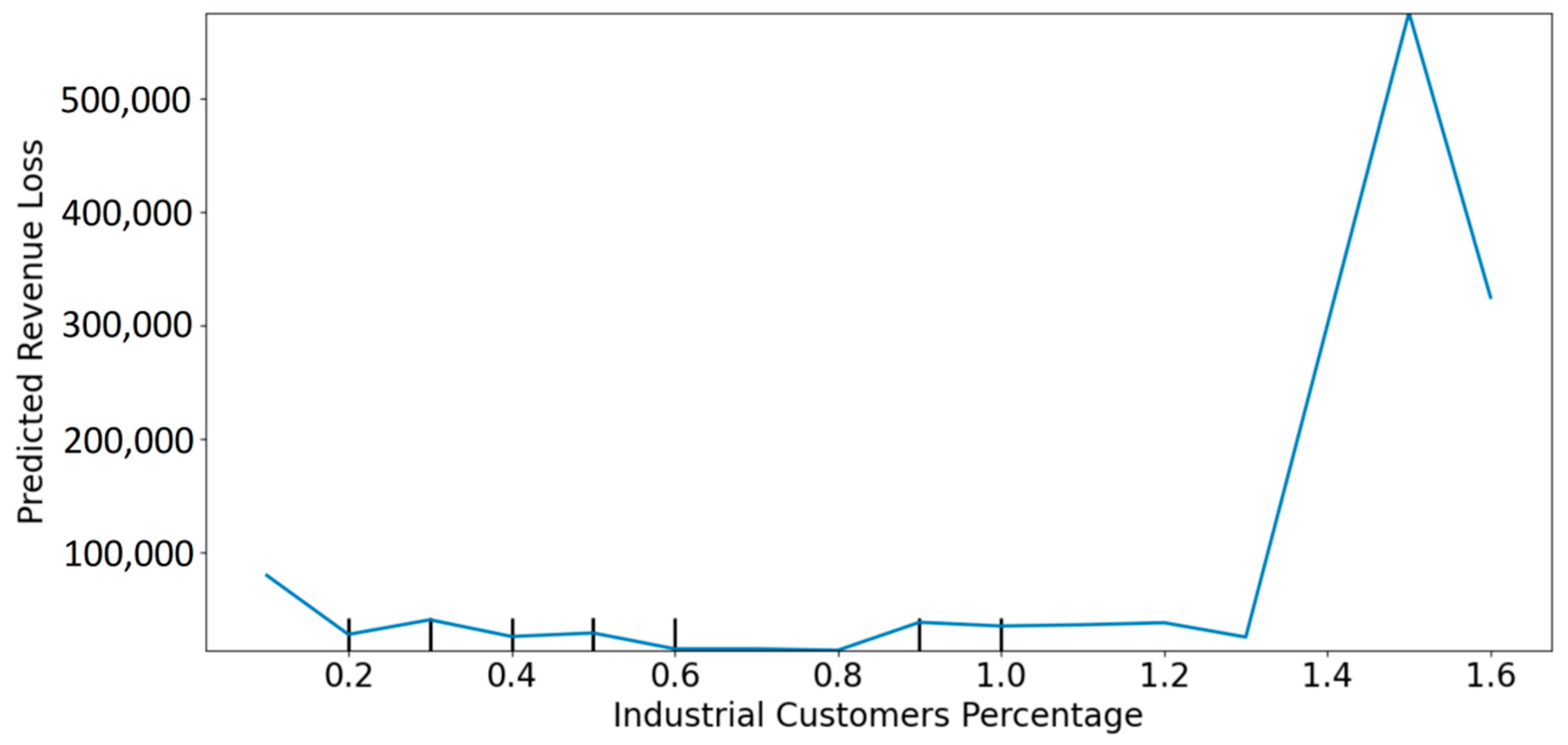
The second important feature is the percentage of industrial customers. The PDP of this feature variable is shown in Figure 21. The predicted revenue loss over the range of this variable is low and almost constant. A peak in the predicted loss is observed when the industrial customer percentage reaches 1.5, while it remains low otherwise. The normalized feature importance of the industrial customer percentage on the predicted loss is 0.13.

The QQ plot between industrial customer percentage and revenue loss is shown in Figure 22. The points forming horizontal lines in the plot indicate the presence of multiple observations of revenue loss against a single observation of industrial customer percentage. This is because such percentages remained the same over the period of a year, when multiple outages occurred and resulted in different revenue losses.

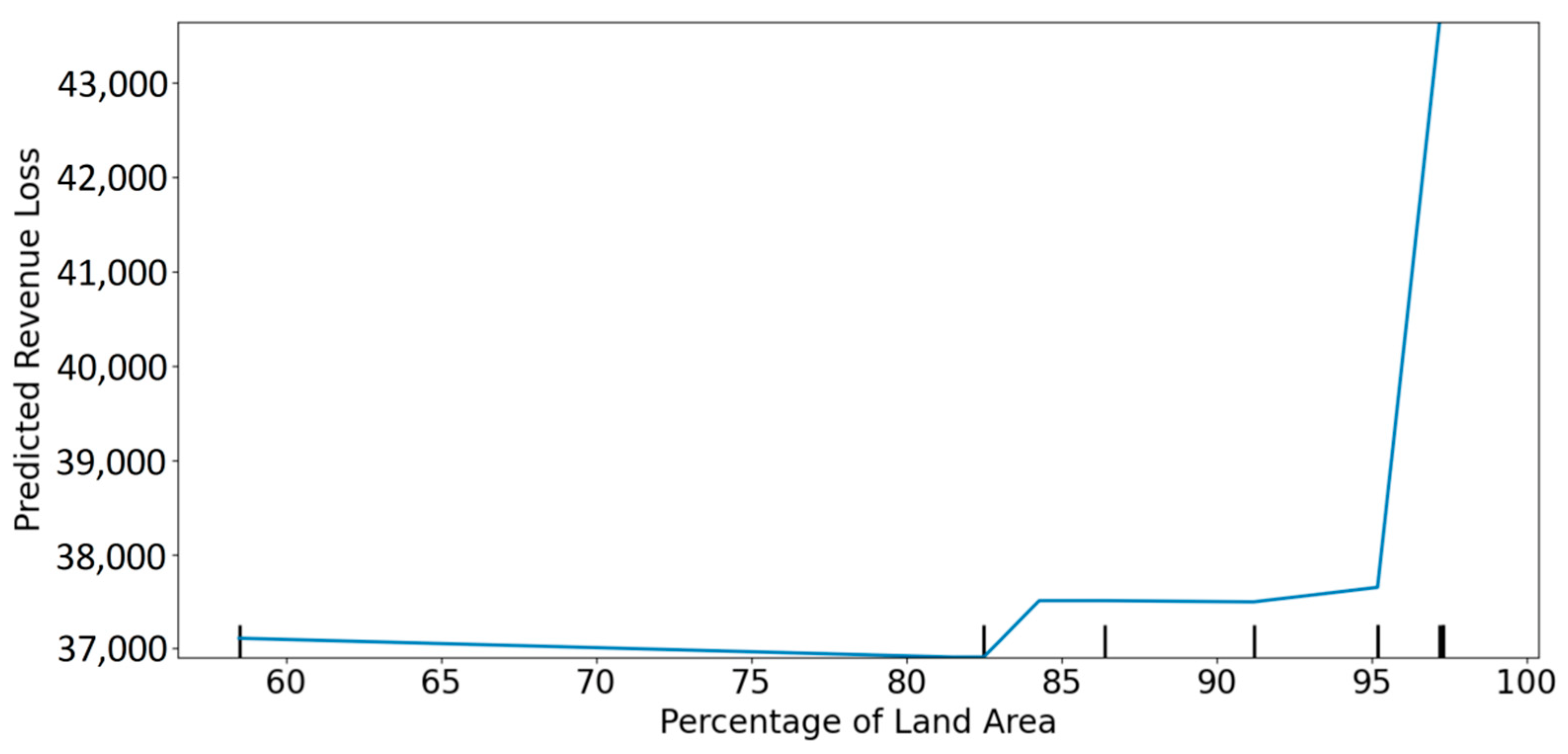
The third important parameter is percentage of land area in the region. It can be observed from Figure 23 that while the land area in the region remains between 60% and 82%, the predicted revenue loss is low. The predicted loss is higher but remains almost constant for the region with land area between 82% and 95%. For the regions with land area more than 95%, the loss shoots up instantly. It is also noteworthy that the deviation in the predicted loss remains smaller for this variable compared to the top two feature variables. The normalized feature importance for percentage land area is 0.12.

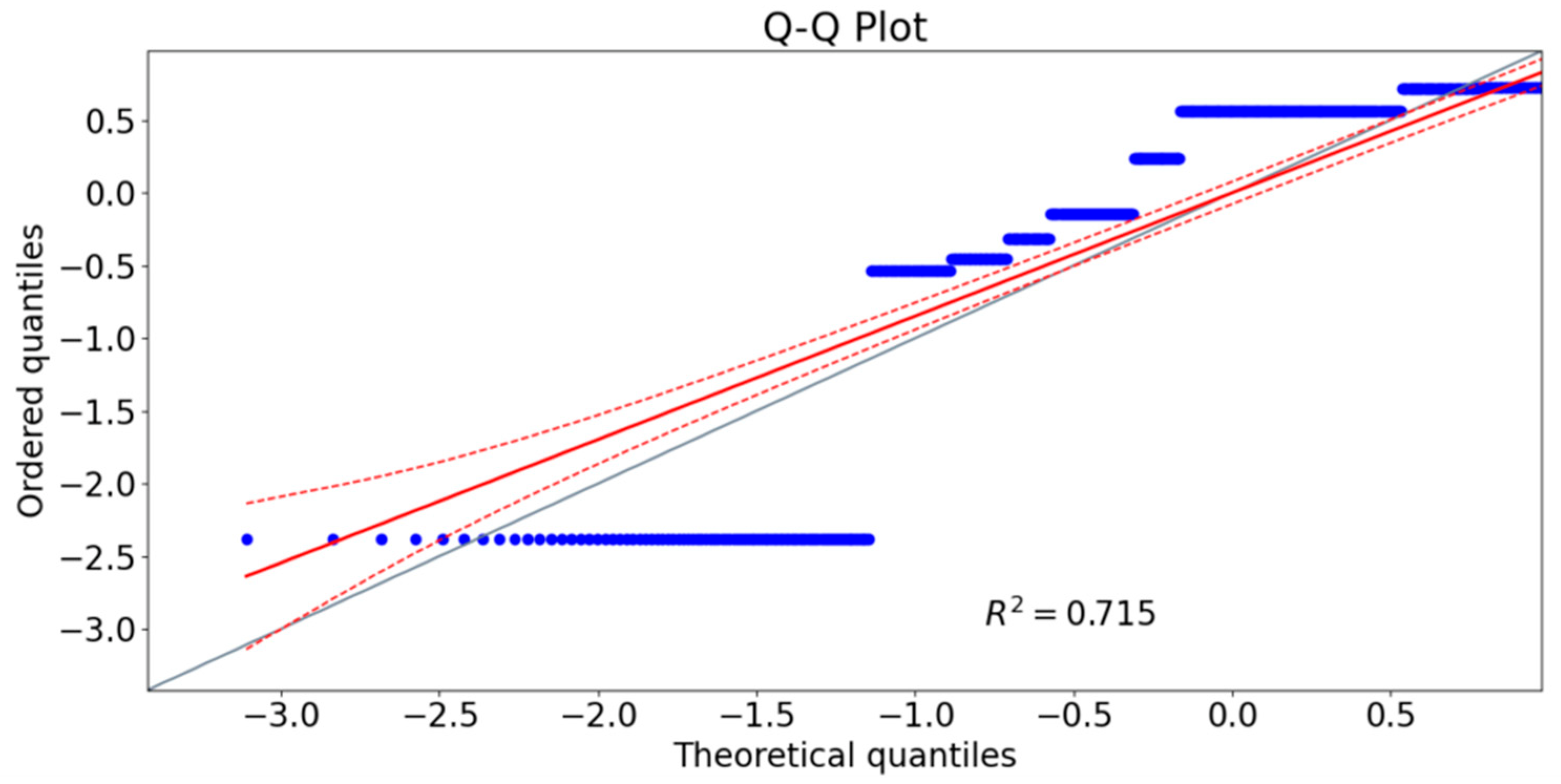
Figure 24 shows the QQ plot between land area percentage and predicted revenue loss. The points forming the long horizontal line in the bottom left quadrant of the plot indicate that the distribution of revenue loss is highly dispersed compared to the percentage of land area. The low value of R² indicates that the model will capture the variance in the data poorly compared to the top two variables.

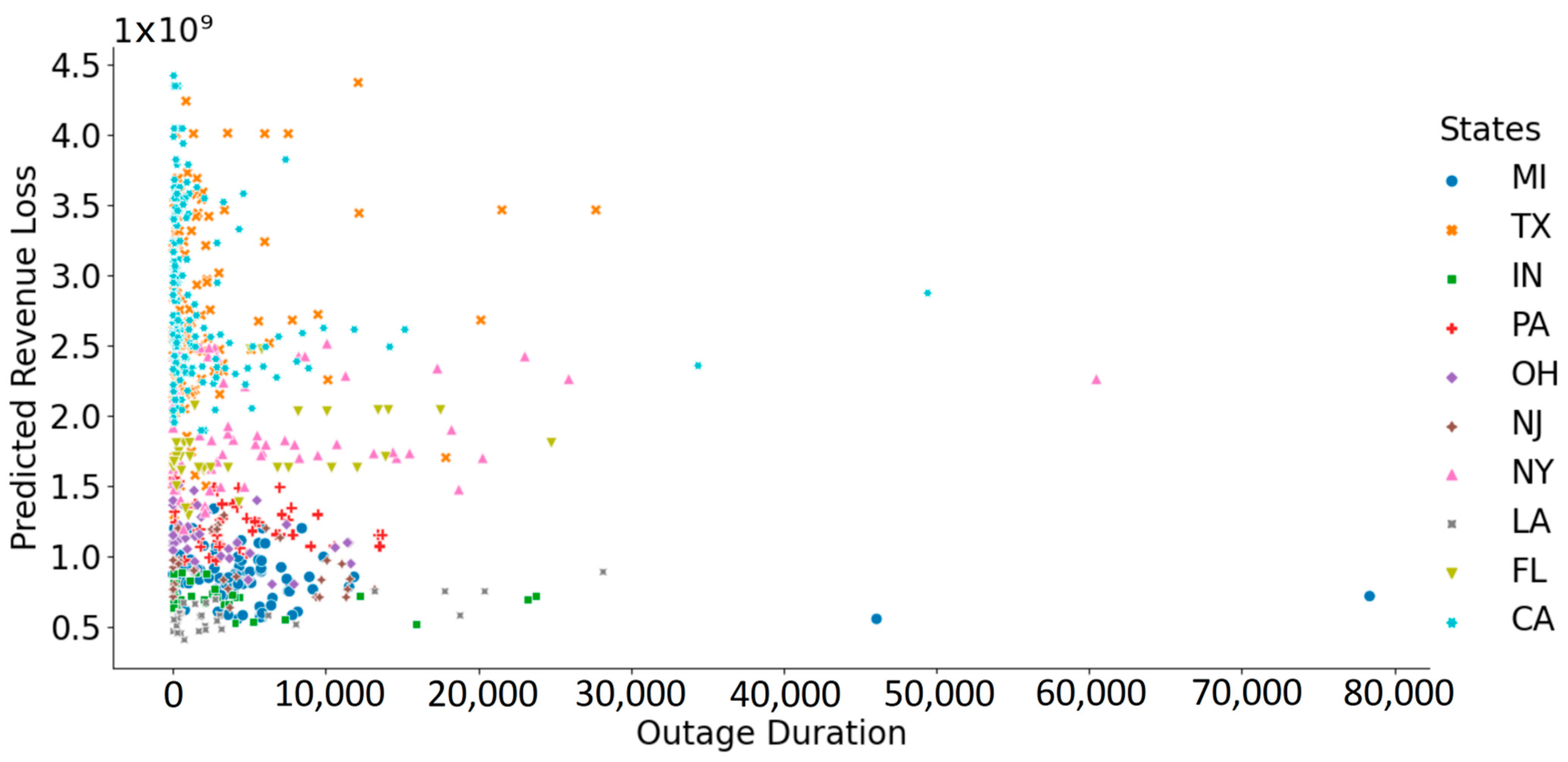
Finally, the scatter plot between the total loss and the outage duration is presented in Figure 25. It can be observed that for the state of California (CA), the largest financial losses are recorded, even for a small duration of power outages. This is because of the elevated prices of electricity in this state, as well as the high sale of electricity. In contrast, the financial losses for the state of Indiana (IN) are low despite the occurrence of long-duration power outage events. The reasons for this are the low prices and the small sale figures.

The revenue loss prediction results reveal that, on average, each increment of 10 min in outage duration will cause a revenue loss of USD 225 million based on the data of the top 10 states combined. Overall, the U.S. bore an average loss of USD 55,190 million per outage event during 2000–2016, where a mean revenue loss of USD 93,717.7 million is estimated for the top 10 affected states of the U.S. per outage event. Undoubtedly, there will be interesting and substantial observations from each state of the U.S. if state-level financial loss prediction is performed; however, this is beyond the scope of this paper and can be considered for future work.

The data of power outage events used in this study belongs to the revenue-loss-based top 10 affected states of the Unites States of America. Therefore, the results are reliable for the prediction of revenue loss in those states. However, the proposed model can be used for any region of the world. The results will vary depending on the nature of available data. This study will be helpful for regulatory authorities in general to make risk-informed decisions, and in particular, for power-supplying enterprises making stock investment decisions and identifying safer investment avenues.

6. Conclusions

In this paper, revenue loss due to non-sale of electricity caused by power outage events in the United States has been predicted. The exploratory data analysis revealed that weather-related natural disasters caused half of the total outage events that occurred, and more than 2/3 of total revenue loss. It was observed that in just 10 of the 50 States, the power suppliers suffer 85% of the total revenue loss of the U.S. The individual consumer sectors were analyzed to gain insight into sector-specific revenue loss, where it was found that the commercial sector was mostly affected. The prediction of revenue loss was performed collectively for the top 10 ranked states using machine learning algorithms, and over 80% accuracy was achieved. It was estimated that revenue of USD 1.35 billion is lost for every hour of power outage in the top ten states, collectively. The impact of the three most important features on the revenue loss was illustrated via partial dependency plots and QQ plots. The results show that revenue loss is a function of multiple parameters, including electricity sales, the percentage of individual consumer sectors’ customers, the geographical landscape, and the economic indicators; however, a very small correlation was found between the important features and the revenue loss.