Differential Capacity as a Tool for SOC and SOH Estimation of Lithium Ion Batteries Using Charge/Discharge Curves, Cyclic Voltammetry, Impedance Spectroscopy, and Heat Events: A Tutorial

Abstract

State-of-charge (SOC) and state-of-health (SOH) of different cell chemistries were investigated using long-time cycle tests. This practical guide illustrates how differential capacity dQ/dU (capacitance) obtained from discharge curves, impedance spectra, and cyclic voltammograms can be used for the instant diagnosis of lithium-ion batteries without fully charging and discharging the cell. The increase of dU/dQ is an early indicator of upcoming heat events and deep discharge. The criterion dQ/dU = dU/dQ = 1 could serve as an indicator for “full charge”. The frequency response of capacitance correlates with the available charge of the battery and reflects overcharge events and deep discharges long before the battery fails. It is not necessary to measure down to extremely low frequencies because the charge transfer pseudocapacitance of around 10 Hz reflects well the SOC. Computer-aided calculation methods for the evaluation of measurements in industrial environments and for the training of students are presented.

1. Introduction

In recent years, the monitoring of lithium-ion batteries [1,2] under normal and hazardous operating conditions has become increasingly important, whether in technical applications or for the development of new materials in laboratory cells (e.g., [3,4,5]). For SOC and SOH estimation, charge–discharge curves are traditionally used, and more recently also impedance spectra. For battery diagnostics, data evaluation with the so-called “differential capacity” is particularly suitable, since dQ/dU is accessible both with DC and AC techniques.

After long periods of rest without power supply, after heavy loads in electric drives, or as emergency power supply in aircraft, the actual state-of-charge (SOC) and state-of-health (SOH) of lithium-ion batteries is often unclear. Determining the capacity and recharging of a 2 Ah battery using the constant current discharge method and other state-of-the-art tools takes from about 1.5 to 2 h. In aviation, fast discharging is allowed only in emergencies, and fast charging is limited to 1C at normal temperatures, and much less than 1C in cold conditions. What is sought is a reliable method for rapid battery diagnosis that reflects at least the upper SOC range.

Our previous work [6,7,8,9] suggested frequency-dependent pseudocapacitance won by impedance spectroscopy as a useful SOC indicator for batteries. Capacitance does not necessarily have to be measured down to extremely low frequencies. Impedance at 0.15 Hz covers a part of the mass transport limited charge storage process by lithium ion intercalation at very low frequencies. The prediction error for C (0.15 Hz) of lithium-iron phosphate (LFP) is better than 1% for a quadratic calibration, and less than 36% for a linear model. For lithium-ion chemistries without a flat discharge curve, the linear trend between the capacitance and the SOC is lost if the slope of voltage versus the SOC changes. With nickel manganese cobalt (NMC), the high impedance modulus correlates with a high SOC above 70%.

In this study, the entire battery operation between the overcharge and deep discharge is considered. The concept of pseudocapacitance [10,11] is highlighted in detail and supported by the statistical evaluation of life tests on new and aged lithium-ion batteries.

A generalized absolute state-of-charge is complicated by the various cell chemistries of lithium-ion batteries. The current state-of-the-art [12,13] does not provide a universal and rapid method of determining the state-of-health of a battery without carefully examining the degradation of hundreds of full charge/discharge cycles. Cell voltage is an uncertain measure of the ‘true’ electric charge. A physical quantity is required that represents the charge state as linearly as possible over a large measuring range.

2. Experimental Section

The batteries investigated in the course of long-time tests under real conditions as in the airplane are compiled in

Table 1. Lithium-ion batteries in this study according to manufacturers’ data sheets.

Chemistry		Cell	Rated	Max./Min.	Capacity	Allowed Current (A)
			Voltage	Voltage U (V)	Q (Ah)	Charge	Discharge
1	LFP	LithiumWerks (A123) ANR26650M1B	3.3	3.6 … 2	2.6	10 (4C)	50 (20C)
2		VoltSolar IFR 18,650 (LiFePO4)	3.2	3.6 … 2	1.5	1.5	4.5 (3C)
3	LMO	Sony US14500VR2B (LiMn2O4 spinel)	3.7	4.2 … 3	0.7	0.7	2
		Samsung INR18650-20F	3.7	4.2 … 2.75	2.0	1	4
4	NMC	Samsung INR18650-20R (LiNiMnCoO2)	3.6	4.2 … 2.5	2.0	1 … 4	22
5		LG ICR18650HE2	3.65	4.2 … 2.0	2.5	4	20
6	LCO	Sanyo/Panasonic UR18650FK, Li1−xCoO2	3.7	4.2 … 2.5	2.3	2.3	4.8
7	NCA	SONY US18650VTC6	3.65	4.2 … 2.0	3.0	5	20
8		Panasonic NCR18500A (LiNiCoAlO2)	3.65	4.2 … 2.5	2.0	1.4 (0.7C)	3.8

.

The proposed calculation methods work with general laboratory equipment and do not require devices from specific manufacturers. In this study, DC power source (Elektro-Automatik EA-PS 2342-10B, Viersen, Germany), electronic load (ET Systems ELP/DCM 9712C, Altlußheim, Germany), impedance spectrometer BIM2 (BRS GmbH, Stuttgart, Germany), and data logger (Agilent 34972A, Meilhaus Electronic GmbH, Alling, Germany) were combined in a climatic chamber (Vötsch VT7021, Balingen, Germany). The surface temperature of the batteries was measured using a linear sensor (Maxim Integrated DS18B20, Mouser Electronics, München, Germany). The temperature sensor was glued to the battery housing using thermal paste and adhesive tape. A second sensor recorded the ambient temperature. The sensors were read out with the help of a Raspberry Pi microcomputer. The difference between the two measured values was evaluated (see Section 4). The cells were charged and discharged at a 1C rate between the upper and lower cutoff voltage at constant ambient temperature in a climate chamber. The battery’s capacity Q₀ was determined by coulomb counting (by a full charge and a full discharge).

For impedance spectroscopy, the fully charged battery was discharged in 2% steps using constant current from SOC 100%, 98%, 96%, down to 30%. After a 20 min rest period to set a stationary cell voltage, the EIS measurement took 80 s for 6 values per frequency decade in the frequency range from 1 kHz to 0.1 Hz. The batteries were aged by charge–discharge cycles between SOC 100% and SOC 80% (DOD 20%), and by deep discharge (DOD 100%). The state-of-health gradually deteriorates, as shown in Figure 1. To quantitatively compare the partial discharge and the deep discharge cycles on an “effective scale”, DOD 20 cycles were weighted by a factor of 1/5 compared to DOD 100 (factor 1). LFP shows the best aging stability and internal resistance.

3. Methodology: Numerical Calculation of Capacity and Capacitance

3.1. Definition of Charge and Aging Indicators

In the following, calculation methods are given for practical use, allowing the reader to apply the proposed methods to their own data sets.

The state-of-charge (SOC) [14]—as used in Figure 2—is defined by the ratio of the currently withdrawn electric charge Q and the total stored capacity Q₀ at the previous full charge. SOC = 1 represents full charge, and SOC = 0 is the empty battery.

Usually, the battery is charged at a constant current until the upper voltage limit is reached. As well, lithium-ion batteries are not allowed to be discharged below the cut-off voltage. The SOC value is valid for a certain time t since the last charge (t = 0). The depth of discharge (DOD) is the percentage of electric charge which is removed from the fully charged battery.

$$\mathrm{SOC}\left(t\right)=Q\left(t\right)/Q_0=1-\mathrm{DOD}\left(t\right)$$

(1)

The state-of-health (SOH) indicates the aging of a battery, expressed as the quotient of the available capacity Q₀ of the fully charged, aged battery and the capacity of the new cell in the first cycle (n = 1). Frequently, the SOH is plotted as a function of the number of charge/discharge cycles n.

$$\mathrm{SOH}\left(n\right)=Q_0\left(n\right)/Q_0\left(1\right)$$

(2)

Coulombic efficiency, also called faradaic efficiency or current efficiency, is the ratio of the released charge Q from the full battery to the total charge Q₀ put into the empty battery. η is large if the battery loses little capacity during each charge/discharge cycle.

$$\mathsf{\eta }\left(n\right)=Q\left(n\right)/Q_0\left(n\right)$$

(3)

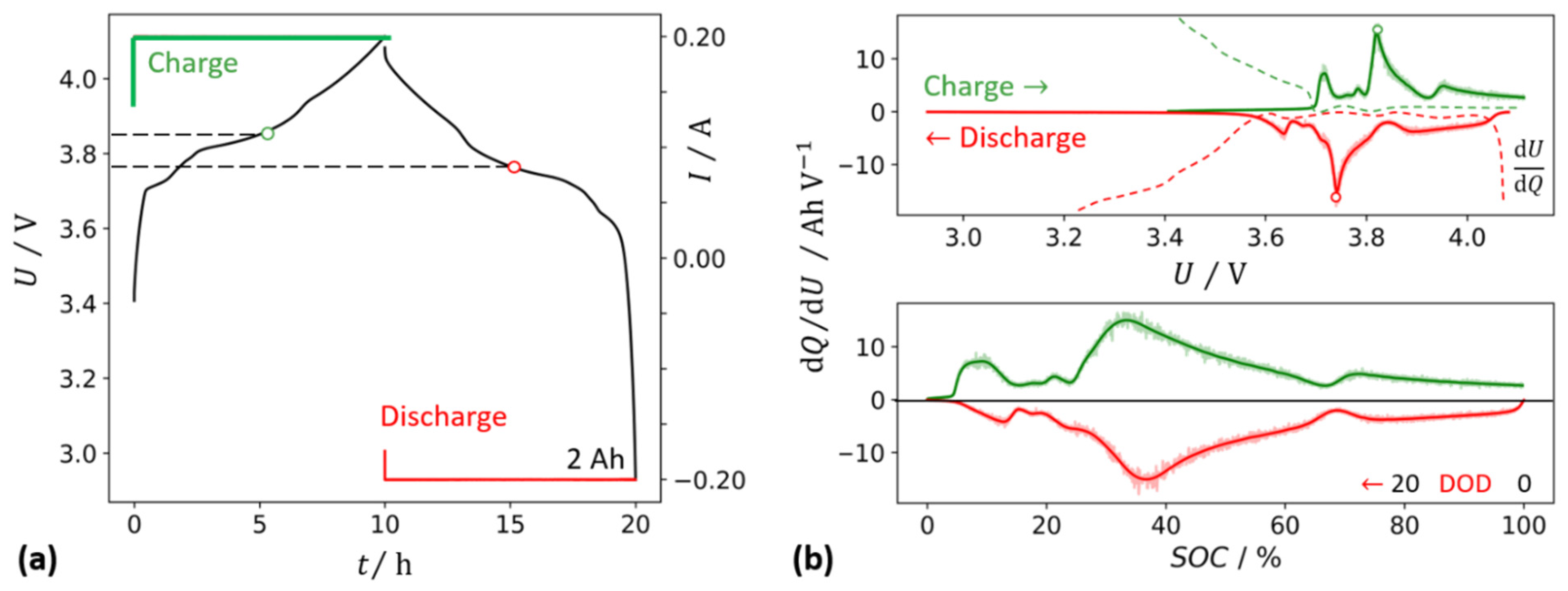
3.2. Calculation of Differential Capacity from Charge–Discharge Curves

What is differential capacity and how is it calculated? “Differential voltage analysis” (temporal change of −Q₀ ⋅ dU/dQ versus capacity Q) was proposed by Bloom et al. [15] to characterize lithium-ion cells in terms of performance and cycle and calendar life.

The reciprocal, differential capacity dQ/dU (also called incremental capacity analysis, ICA [16]), in Figure 3, reflects the slope of the flat regions of charge–discharge characteristics (ΔU → 0). The unit dQ/dU indicates small changes of the battery during aging better than the U(Q) curve. The unit dQ/dU is Farad: F = C/V = As V⁻¹. Therefore, the symbol C is used for an electrical capacitance, which must not be confused with the electrical charge (capacity Q).

$$C=\frac{\mathrm{d}Q}{\mathrm{d}U}\approx \frac{\mathsf{\Delta }Q}{\mathsf{\Delta }U}$$

(4)

Electric charge Q(t) is calculated by integrating the current I(t) with respect to time t, for example, using the trapezoidal rule. N is the number of measured values from the beginning of charge or discharge (i = 1) to the desired time t_i (i = N). The approximation is valid for a data set with small equidistant time intervals, $h=t_i-t_{i-1}<0,1 \mathrm{s}.$ By definition, charging currents are positive (I > 0), discharging currents have negative sign (I < 0).

$$Q\left(t_i\right)=\underset{0}{\overset{t_i}{{\displaystyle \int }}}I\left(t\right) \mathrm{d}t={\displaystyle \sum }_{i=2}^N\frac{I_i+I_{i-1}}{2}\cdot \left(t_i-t_{i-1}\right)\approx h{\displaystyle \sum }_{i=2}^N{I}_i$$

(5)

The calculation is easily done with the PHYTON function:

Q = numpy.append([0],scipy.integrate.cumtrapz(I, t))

Differential capacity (capacitance), C = dQ/dU, is obtained by numerically differentiating the electric charge Q(t) with respect to the instantaneous voltage U(t), in the simplest case by applying the differential method.

$$\frac{\mathrm{d}Q}{\mathrm{d}U}=\frac{Q\left(t_{i+1}\right)-Q\left(t_{i-1}\right)}{2h}+\mathcal{O}\left(h^2\right) \approx \frac{Q\left(t_{i+1}\right)-Q\left(t_i\right)}{U\left(t_{i+1}\right)-U\left(t_i\right)} \mathrm{at} \overline{U}=\frac{U_{i+1}+U_i}{2}$$

(6)

Professional program packages use interpolation polynomials for a given number of interpolation points, e.g., the Savitzky–Golay method.

The calculation is easily done with the PHYTON function:

dQdU = numpy.gradient(Q, U)

3.3. Calculation of Differential Capacity Avoiding Numerical Problems

What is the difference between capacity and capacitance? What to do when dividing by zero ΔQ/ΔU if the voltage does not change between two readings?

For constant current charge and discharge, numerical problems with small voltage differences can be avoided by using the reciprocal of the differential capacity. In Equation (7), the differential capacity dQ/dU = capacitance C formally reflects the change of cell conductance (ΔR)⁻¹ multiplied by the time interval Δt.

The unit Farad reads: F = As/V = Ω⁻¹ s.

$$C=\frac{\mathrm{d}Q}{\mathrm{d}U}={\left(\frac{\mathrm{d}U}{\mathrm{dQ}}\right)}^{-1}={\left(\frac{\mathrm{d}U}{\mathrm{d}\left(It\right)}\right)}^{-1}={\left(\frac{\mathrm{d}R}{\mathrm{d}t}\right)}^{-1}$$

(7)

Differential capacity dQ/dU shows a peak for every flat section of the charge/discharge curve U(Q), see Figure 4.

On the other hand, the reciprocal dU/dQ reflects the steepest decent. The minima of dU/dQ are the maxima of dQ/dU, and vice versa. The logarithmic scale log (dU/dQ) provides no additional insight. Unfortunately, the differential capacity peaks do not directly indicate the actual state-of-charge. The criterion dQ/dU = dU/dQ = 1 could at best serve as an indication that the battery is practically fully charged.

How are resistance and capacitance related? Attempt at an explanation: By recording the time constant τ during charging and discharging of a real storage device, a characteristic value R (dissipative property) and a general storage characteristic value C = τ/R (conserving property) are obtained. Although both C and R are related to each other over time, and they physically originate from two different phenomena: C is the capacitance of an energy storage device (in equilibrium) and R is the resistance of an energy converter from electrical energy to thermal energy (in nonequilibrium). In this respect, one is used to calculate the other, but they are two properties of the same component. Resistance is described by a gradient law (dissipative), whereas capacitance is described by a law of storage (conserving). Apart from the metrological interpretation, the product conductance times time has no further electrical significance.

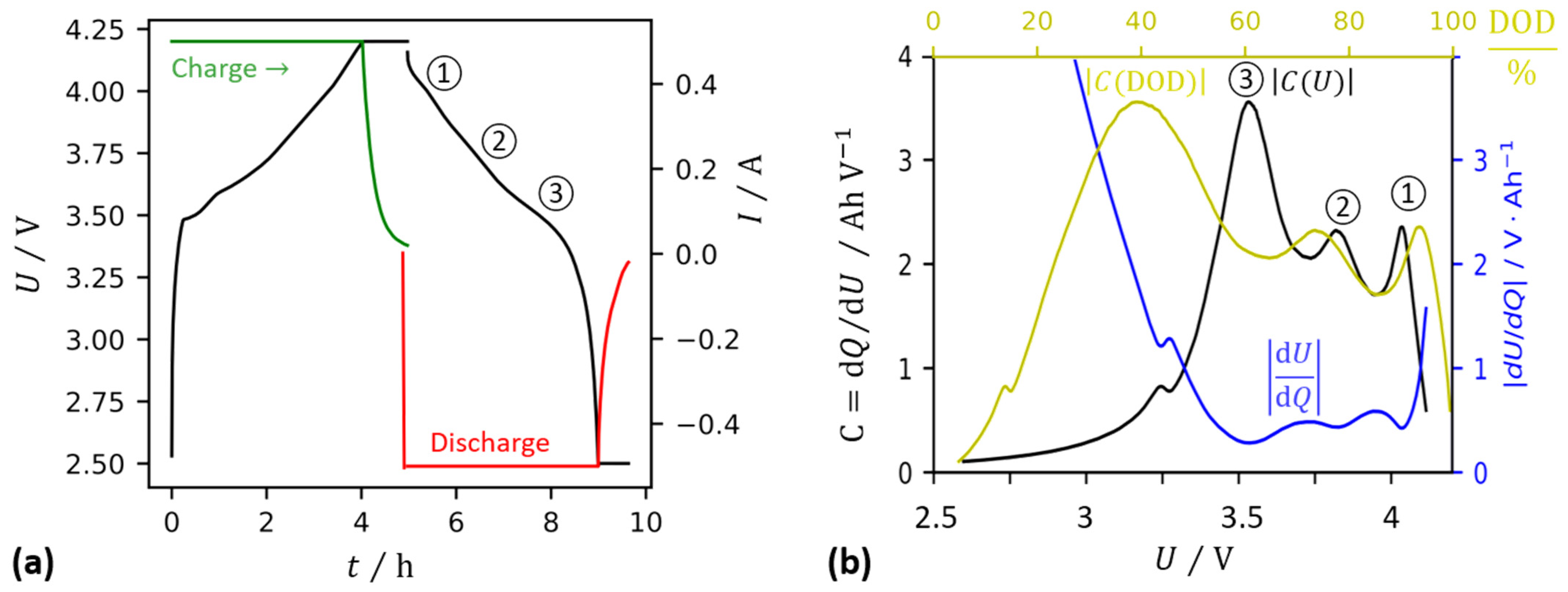
3.4. Calculation of Voltammetric Capacitance

Figure 5 shows the familiar cyclic voltammogram of a platinum electrode in a three-electrode configuration. However, differential capacity was calculated for the cyclic voltammogram (C = I/v, Equation (8)) and the constant current measurement (C = dQ/dU, Equation (7)).

The phenomenon that double-layer capacitance C is not a constant quantity but depends on the applied electrode potential φ that was studied already in the 1940s at mercury surfaces in aqueous salt solutions (Grahame [17]). At the potential-of-zero-charge, the electrode surface is not electrically charged, and the capacitance of the double-layer is smallest. The cyclic voltammogram of a platinum electrode [18] in aqueous solution shows that differential capacity = capacitance C (in F) is directly proportional to the charging current I (in A) at a given electrode potential E and voltage scan rate v (in V/s) [19].

$$C=\frac{\mathrm{d}Q}{\mathrm{d}E}=\frac{I}{\mathrm{d}E/\mathrm{d}t}=\frac{I}{v}$$

(8)

Q is the electric charge (in As) and t is the time (in s). The current I is composed of the capacitive part of the double-layer charging and discharging and the faradaic component of battery-like redox reactions: I = I_C + I_F. While the capacitive current varies with v and becomes important at high scan rates (I = C · v), the faradaic peak current, which must always be measured from a baseline of charging current, varies with I ∼ v^1/2 for linear diffusion.

The oxygen reduction (O₂ + 4 e⁻ + 4 H⁺ → 2 H₂O) in the galvanostatic measurement shows a prepeak of the same shape; this means: both the dissolved and adsorbed species are electroactive, and the reduced product species, is strongly adsorbed (Bard [19]).

In electrochemical equilibrium, potentiostatic and galvanostatic measurements give the same results as long as the control loop of the cell is stable. This consistent result makes it clear that potentiodynamic and quasi-stationary galvanostatic measurements can be correctly compared on the voltage scale.

3.5. Calculcation of Pseudocapacitance from Impedance Spectra

The real part of the impedance (resistance R = Re Z) and the modulus |Z(ω)| reflect the electrolyte and the kinetic inhibitions of the electrode processes, whereas the imaginary part (reactance) is attributed to the double-layer and adsorption phenomena [20]. Several methods for the SOC and SOH estimation using impedance spectra have been proposed in the literature [21,22,23]. Reliable methods of health assessment and fault diagnosis, such as overcharge and deep discharge, require a deep understanding of the impedance spectrum, which has not been proposed so far.

As shown earlier [6], the pseudocapacitance C(ω) [11] according to Equation (9) is a unique measure for the activity of the electrode/electrolyte interface and works as a qualitative indicator of the battery’s state-of-charge.

$$C\left(\mathsf{\omega }\right)=\mathrm{Re} \underset{\_}{C}\left(\mathrm{j}\mathsf{\omega }\right)=\frac{\mathrm{Im} \underset{\_}{Y}\left(\mathrm{j}\mathsf{\omega }\right)}{\mathrm{j}\omega }=\frac{-\mathrm{Im} \underset{\_}{Z}\left(\mathrm{j}\mathsf{\omega }\right)}{\omega \cdot {\left|\underset{\_}{Z}\left(\mathrm{j}\mathsf{\omega }\right)\right|}^2}\approx \frac{-1}{\omega \cdot \mathrm{Im} \underset{\_}{Z}\left(\mathrm{j}\mathsf{\omega }\right)}$$

(9)

The approximation holds for high frequencies and negligible internal resistance. At frequencies above 5 kHz, pseudocapacitance C approaches the geometric double-layer capacitance, C_D = C(ω → ∞). At low frequencies, pseudocapacitance approaches the DC value of capacitance, which reflects the maximum useable storage capacity of the device.

The electrolytic double layer, the charge transfer reaction by absorbed ions on the electrode surface, and lithium ions intercalating into the porous electrodes cause the capacitive properties of cell impedance in three different frequency ranges (see Section 4).

A large pseudocapacitance indicates a high SOC, while the imaginary part of impedance represents the inverse of SOC. Overcharging disrupts the linear trend between capacity and SOC. The linearity between pseudocapacitance and electric charge is improved when the electrolyte resistance (intersection with the real axis) is corrected. This defines a set of congruent curves which are independent of contact and cable errors.

$$R\left(\omega \right)=\mathrm{Re} \underset{\_}{Z}\left(\omega \right)-\mathrm{Re} \underset{\_}{Z}\left(\omega \to \infty \right)$$

(10)

4. Results and Discussion: Charge–Discharge Curves

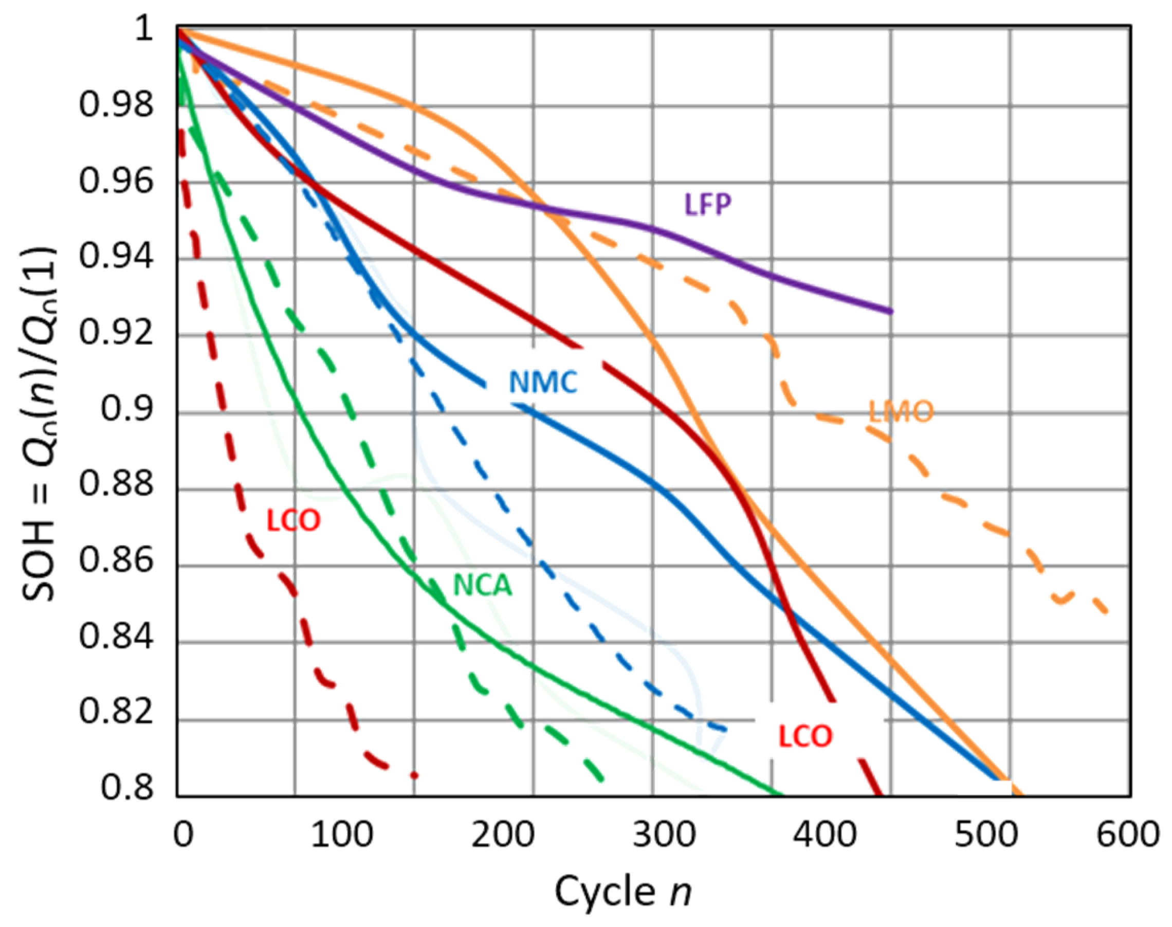
4.1. How Differential Capacity Indicates Different Cell Chemistries

In this section, the suitability of capacitance = differential capacity dQ/dU as a quality criterion for the state-of-charge, (SOC), state-of-health (SOH), thermal events, and the cell chemistry is to be clarified by experimental charge–discharge curves in the regular operating range, in overcharge and the deep-discharge region. Charge–discharge characteristics are shown in Figure 6.

For different cell chemistries, constant current characteristics were recorded using a constant current load (Keithley SMU 2400).

• Charge: → CC 0.5 A up to 4.2 V; CV: cut-off current <20 mA (SOC = 1).
• Discharge: → CC 0.5 A to cut-off voltage 2.5 V; CV: cut-off current 20 mA (SOC = 0).

At a constant charge and discharge current, respectively, the electric charge and energy increase and decrease linearly with time: Q ∼ t and QU ∼ t. Depending on the cell chemistry, the number and positions of the measured dQ/dU peaks differ. Differential capacity is more distinct and sharper on a voltage scale than against SOC. The voltage positions of the dQ/dU peaks are well reproducible and differ only slightly for individual batteries of the same type (ΔU ≈ ±0.02 V). The signals correlate with the redox processes of the cell chemistry, so that Figure 6c allows an interpretation similar to that of the cyclic voltammogram.

The distance between charge and discharge signal is about 0.1 V, which is due to the internal resistance of the battery. With larger charge currents, the dQ/dU peaks shift toward higher voltages. With larger discharge currents, the dQ/dU peaks shift toward lower voltages (

Table 2. Differential capacity peaks dQ/dU at three currents of different lithium-ion chemistries.

Battery	Current	Voltage Position at Charge (V)						At Discharge (V)				Discharge Efficiency
	(A)	1	2	3	4	5	6	1	2	3	4	Ah/Ah	V/V	Wh/Wh
Panasonic	0.25	3.41	3.50	3.62	3.79	3.92	4.13	3.28	3.56	3.85	4.06	0.98	0.95	0.93
NCR18500A	0.5	3.48	3.55	3.60	3.81	3.94	4.17	–	3.53	3.82	4.03	0.99	0.90	0.89
2 Ah, 3.7 V, LCA	1.0	–	3.52	3.63	3.73	3.98	–	–	3.50	3.76	4.00	0.97	0.85	0.83
Average position (in V)		3.45	3.52	3.62	3.78	3.95	4.15	3.28	3.53	3.81	4.03
Error (95% conf.)		±0.48	±0.07	±0.04	±0.10	±0.07	±0.22	–	±0.08	±0.10	±0.08
Sony	0.25	3.66	3.74	–	–	–	–	3.54	–	–	–	0.95	0.89	0.84
US14500VR2	0.5	3.60	3.72	–	–	–	–	3.51	–	–	–	0.98	0.85	0.83
0.7 Ah, 3.6 V, LMO	1.0	3.74	3.85	–	–	–	–	3.42	–	–	–	0.97	0.78	0.76
Average position (in V)		3.67	3.77					3.49
Error (95% conf.)		±0.18	±0.17					±0.16
IFR 18500	0.25	3.30	3.39	3.41	–	–	–	3.21	3.26	3.26	–	0.90	0.90	0.815
1.2 Ah, 3.2 V, LFP	0.5	–	3.35	3.45	–	–	–	3.21	–	–	–	0.93	0.84	0.78
	1.0	–	3.39	3.49	–	–	–	3.13	–	–	–	0.92	0.79	0.73
Average position (in V)		3.30	3.38	3.45				3.19	3.26	3.26	–
Error (95% conf.)		–	±0.05	±0.11				±0.04	–	–	–

). Coulombic efficiency (output charge/input charge), voltaic efficiency (average discharge voltage/average charge voltage), and energetic efficiency (energy output/input energy) also decrease slightly with increasing discharge current.

4.2. How Differential Capacity Indicates Aging

What is the benefit of differential capacity? Is it better to plot dQ/dU against cell voltage or against the state-of-charge?

The maxima of charge and discharge lie at different voltages due to the internal resistance of the battery.

Table 3. Voltage positions (in V) and peak shift of the differential capacity dQ/dU of aged batteries.

Battery	Residual	Charge			Discharge			Mean Peak
	Capacity (Ah)	1	2	3	1	2	3	Difference
SANYO R18650F (2.3 Ah, LCA)	2.26	3.71	3.82	3.96	3.63	3.74	3.91	0.07 ± 0.02
	2.13	3.75	3.87	4.00	3.65	3.73	3.94	0.10 ± 0.04
	2.10	3.78	3.89	4.03	3.63	3.73	3.94	0.13 ± 0.04

shows the shift in dQ/dU peak values for three old LCA batteries of the same type but with highly different aging history.

Aging increases the distance between the corresponding constant current charge peaks and discharge peaks. Hence, the voltage distance between corresponding charge and discharge peaks is a measure of increasing cell resistance, dQ/dU (charge) − dQ/dU (discharge) ∼ ΔR.

In lifetime tests, according to Dubarry et al. [16], a shift in the oxidation peaks to higher voltage and the reduction peaks to lower voltage describes this increase of internal resistance ΔR better on the voltage scale than against the SOC (see Figure 3b above). Lithium iron phosphate chemistry, for example, shows a depression of the differential capacity:

• Resistance increase shifts all three dQ/dU charging peaks toward higher voltages.
• Loss of lithium supply or anode material decreases the dQ/dU peak height at 3.4 V.
• Loss of cathode material reduces all three dQ/dU peaks (3–3.5 V).

The gradual capacity fade of lithium-ion batteries [16,24,25] is mainly caused by the negative electrode (anode); it can be attributed to the decomposition of the electrolyte in contact to lithium metal [26], the dissolution of transition metals at the cathode and redeposition at the anode [27], and the steady loss of the electrochemically available lithium in the cell, which prevents the formation of a stable protective layer on the cathode material [28]. For LiCoO₂/graphite cells, the initial cell capacity is determined by the negative electrode, while the positive electrode becomes critical after 500 cycles [29].

4.3. How Differential Capacity Indicates Overcharge and Heat Events

Differential capacity dQ/dU reaches a local maximum near full charge (Figure 6), because cell voltage reaches a constant value (ΔU → 0), which can serve as a criterion that the battery is now fully charged and not yet overcharged. As well, incremental voltage dU/dQ rises abruptly as soon a constant current can no longer be fed into or drawn from the cell (ΔI → 0).

Unfortunately, the dQ/dU peak near the nominal voltage is an inaccurate criterion for the starting point of discharge. However, the intersection of dQ/dU and dU/dQ indicates the full charge (SOC = 1) and the half-full state (SOC = 0.5), see Figure 4 above.

Figure 7 shows the sharp rise in voltage during overcharging. Differential capacity dQ/dU rises moderately, but voltage change dU/dt (or dU/dQ) becomes maximum at 4.2 V and 4.9 V (LCA chemistry).

After the overload protection is triggered, the voltage immediately jumps to the value set as the voltage limit, as the device continues to drive the specified current (CC). The 5 V cell voltage cannot be reached by constant current charge. A soft crackling sound is heard and no more current flows.

During charging, the temperature moderately increases during the initial strongest voltage increase (Figure 6, above). A really sharp rise in temperature is observed shortly before the exhaustion of the battery (Figure 7). The dU/dQ peak is therefore an early indicator for upcoming deep discharge and exhaust heat events—for an explanation, see Section 4.4. Due to the heat capacity and thermal conductivity of the battery, measurable temperature changes on the housing do not occur until some delay after the dangerous voltage rise.

Repeated deep discharge below 2.5 V results in a deterioration without the battery failing. An immediate temperature rise is observed with increasing depth of discharge. Both deep discharge and overcharge do not significantly shift the dQ/dU peaks on the voltage axis.

4.4. How Differential Capacity Depends on Ambient Temperature

The voltage change dU/dt appears to be an early indicator of an impending temperature rise and thermal runaway. Based on the thermodynamic relationship between cell voltage U = ΔE and Gibbs free enthalpy change of the cell reaction ΔG, the temperature increase is likely to reflect an exothermic lattice change ΔH or an entropy increase ΔS.

$$\mathsf{\Delta }G=\mathsf{\Delta }H-T \mathsf{\Delta }S=-z F \mathsf{\Delta }E$$

(11)

The peaks in the dQ/dU curves are from phase equilibria, whereas dU/dQ peaks reflect phase transitions (Bloom [15]). Coexisting equilibrium phases with different lithium concentrations have the same chemical potential (dU = 0). Phase changes in the course of deep discharge cause heat events, and dU/dQ peaks warn of this. With a constant current discharge, dQ is always nonzero.

At constant temperature, old and new cells almost do not differ in the voltage position of the dQ/dU discharge peaks, since the basic electrochemical thermodynamics is the same (Equation (11)). However, the height of the dQ/dU peak becomes smaller with old cells. When charging (CC), the dQ/dU peak of old cells is at a slightly higher voltage. The difference is unfortunately too small to predict a lifetime.

The warmer the environment, the more electrical charge a battery delivers. It is therefore not surprising that the peak values of the differential capacity also shift to higher voltage or state-of-charge (Figure 8).

The central peak of dQ/dU at about 3.25 V could serve as a rough diagnostic criterion for the “half-full” state (SOC = 50%). The “almost empty” state (SOC = 20%) is indicated by the peak at 3.15 V. The third peak shows the “almost full” battery at 3.3 V (SOC = 90%).

5. Results and Discussion: Impedance Spectroscopy

It is known that lithium inventory loss and positive mass loss, as well as impedance growth and capacitance degradation, are worse at high temperature, at higher depth-of-discharge, and at higher average state-of-charge [24,25,26,27,28,29,30].

The aim of this section is to identify the experimental representations of ac capacitance [6] for rapid SOC and SOH determinations at any condition of the cell. Reference values were measured by charge–discharge cycling (Ah counting [31]).

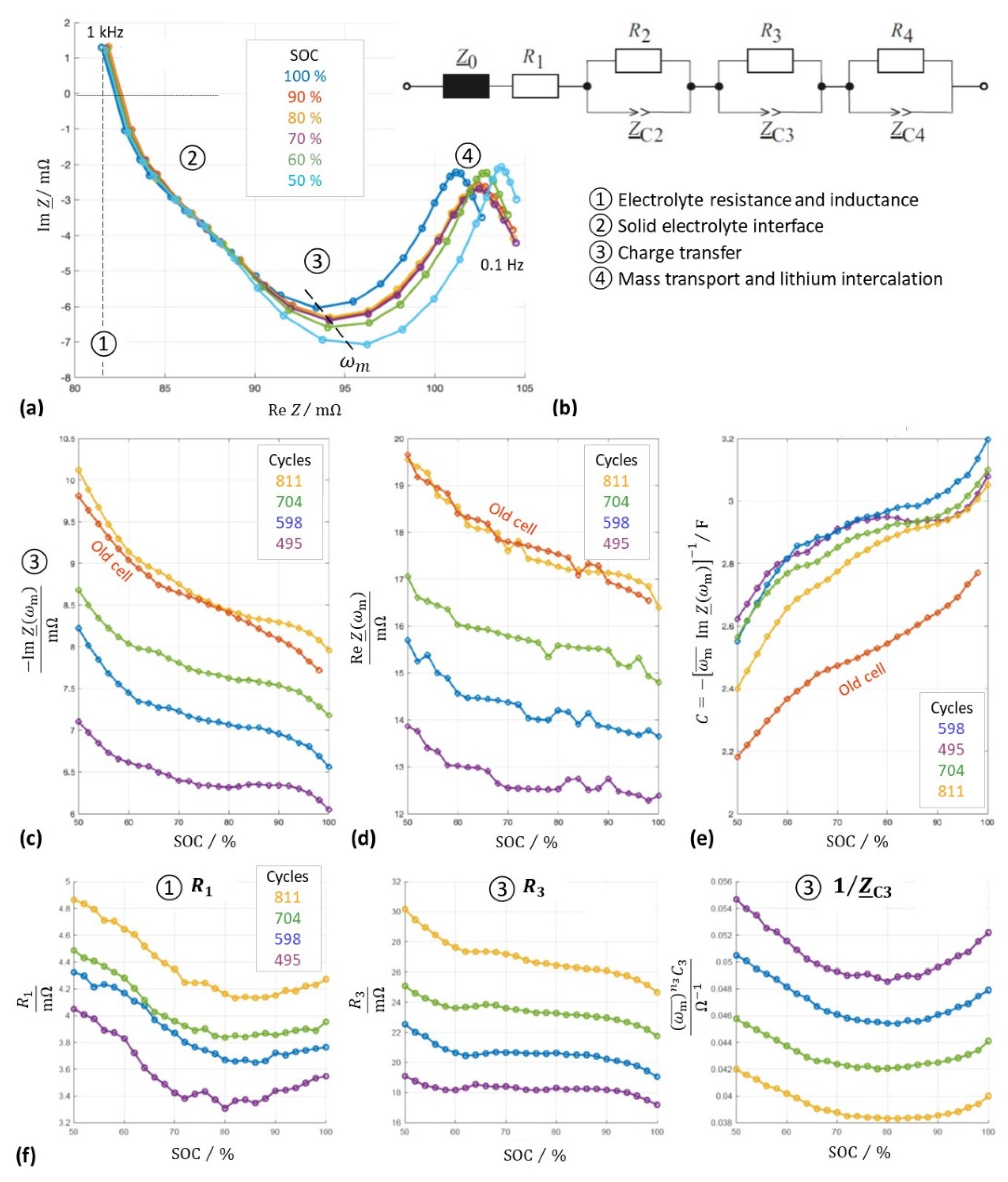
5.1. How Cell Chemistry Coins the Complex Plane Plot

Two questions arise: In which region of the impedance spectrum is the SOC best represented? Additionally: Is rather resistance or capacitance an appropriate measure for the SOH?

Typical impedance spectra of batteries (Figure 9) show three arcs in the complex plane, whereby the state-of-charge affects both the real part and the imaginary part of impedance.

• Electrolyte resistance R_e and the solid–electrolyte interface (SEI) at high frequencies are of little use for SOC determination. Therefore, R_e is subtracted from the real parts (Equation (10)). However, R_e is useful for aging control.
• Charge-transfer at medium frequencies: resistance drops and capacitance according to Equation (9) increases with SOC.
• The shape of pore diffusion and intercalation at frequencies below 0.01 Hz depends on whether the lithium-ions are mobile in linear channels (Li_1−xFePO₄), in areas of the layer lattice (Li_1−xCoO₂, NMC), or in the void spaces of a spinel (Li_1−xMn₂O₄, LMO).

Cell chemistry plays an important role for SOC monitoring [6]:

• LCO shows more or less congruent Nyquist curves. Capacitance best reflects the SOC between 80% and 100%. At medium and low states of charge, resistance and reactance are high when the SOC is low; an illogical order pretends a higher SOC. The helpful relative quantity Im Z(SOC)/Im Z(SOC = 1) misrepresents overcharge and aging phenomena.
• LMO shows a slight increase of reactance (Im Z∼SOC) in the linear range of the flat voltage–charge curve. Below SOC = 0.5, impedance increases strongly.
• With NMC and NCA, high resistance reflects high residual battery capacity (SOC > 0.7). Resistance and reactance are high, when SOC is low (SOC ≤ 0.5).

We conclude, there is no simple method for all lithium-ion chemistries to read the absolute SOC values from the shape of the complex plane plot. Moreover, it is practically impossible to fit all possible impedance spectra to a universally valid equivalent circuit.

5.2. How the Charge-Transfer Semicircle Indicates SOC

In practice, it is cumbersome and time-consuming to measure reliable impedance values at low frequencies in the range of lithium-ion diffusion and intercalation (<0.1 Hz). We have therefore evaluated the real and imaginary parts of impedance at the minimum of the semicircle that is attributed to the charge-transfer reaction at medium frequencies.

For a cycle life test on a new battery, the real part, imaginary part, and the capacitance at the semicircle’s minimum ③ show a clear but nonlinear dependence on the SOC and SOH (Figure 9). The exact circular frequency at the minimum, ${\mathsf{\omega }}_{\mathrm{m}}=2\pi f_{\mathrm{m}}$, was determined by cubic spline approximation. By definition, capacitances have negative imaginary parts, and inductances have positive sign. Learners should not be confused by negative axes and twisted coordinate systems in the literature.

Pseudocapacitance at the semicircle minimum (in mathematical convention) reads:

$$C\left({\mathsf{\omega }}_{\mathrm{m}}\right)=\frac{-1}{\omega \cdot \mathrm{Im} \underset{\_}{Z}\left({\mathrm{j}\mathsf{\omega }}_{\mathrm{m}}\right)}$$

(12)

The charge-transfer reaction follows in good approximation an equivalent circuit of a resistor connected to a lossy capacitance (constant phase element, CPE) in parallel. The semicircle is shifted to the right in the Nyquist plot by the constant resistance R₂ of the passive layer (SEI) and the electrolyte resistance R₁.

$${\underset{\_}{Z}}_3\left(\mathrm{j}\mathsf{\omega }\right)=\frac{1}{\frac{1}{R_3}+\frac{1}{{\underset{\_}{Z}}_{C3}\left(\mathrm{j}\omega \right)}}=\frac{R_3}{1+{\left(\mathrm{j}\omega \right)}^n{C}_3{R}_3}$$

(13)

We conclude that the pseudocapacitance at the minimum of the semicircle C(ω) is an illustrative measure of the SOC. Unfortunately, the frequency ω_m at the semicircle minimum jumps statistically (see Figure 9a) without a clear relationship with the SOC, so the average value of all SOC measurements of the charge–discharge cycle was used as ω_m.

The question arises whether the resistance and the parameters C and n of the CPE element are also suitable for SOC measurement. Figure 9f shows the quantitative rise of charge-transfer resistance R₃, indicating increasing kinetic inhibition both during discharge and by aging. A linear trend of R₃ with the state-of-charge is not evident.

5.3. How the Charge-Transfer Semicircleis Useful for SOH Control

As the battery ages, the resistance R₃ gradually increases due to the active mass loss and volume changes of the jelly roll. Therefore, the resistance at the previous full charge of the battery can serve as a reference condition for the SOH control. Since heat accelerates electrochemical kinetics, R₃ must be corrected to a reference temperature.

In the equivalent circuit (Figure 9b), R₂ maps the active particles on the current support and the solid electrolyte interphase (SEI), which deteriorates with the increasing number of cycles, unfortunately without clear relation to the SOC. In Figure 9, R₂ is constant because all impedance spectra refer to the same cycle. For fit results, see Supplementary Material.

For the SOH control, however, the increase in the electrolyte resistance R₁ and grain-boundary resistance R₂ are useful because they are coupled with electrolyte conductivity and the “unwetting” of the pore spaces by volume expansion of the electrodes (CT scans see Gauthier et al. [13]).

Electrolyte resistance R₁ decreases slightly with increasing temperature due to better ion mobility, but not as much as the charge transfer resistance R₃ decreases (due to faster kinetics according to Arrhenius’ rule: lg k∼1/T).

5.4. How to Combine Capacitance from AC and DC Methods

What is the advantage of combining the pseudocapacitance C(ω) from the impedance measurements with the differential capacitance dQ/dU from the constant current discharge (ICA) curves? In which SOC range does the battery release the most of its stored energy?

Different cell chemistries use different voltage windows for full discharge (

Table 4. Voltage range (in V) as a function of state-of-charge of lithium-ion batteries during discharge.

Chemistry	Battery	Main Discharge		Residual Discharge		Full Discharge		Range
		V	SOC	V	SOC	V	SOC	V/SOC
LFP	LithiumWerks ANR26650M1B	3.7 … 3.3	1 … 0.45	3.3… 3.2	0.25	<3.2	<0.3	0.7
LMO	Sony US14500VR2B (LiMn2O4)	4.1 … 3.5	1 … 0.25	<3.5	<0.25			0.8
NMC	Samsung INR18650-20R (LiNiCoMnO2)	4.1 … 3.6	1 … 0.35	3.6 … 3.4	0.1	<3.4	<0.1	0.6
NCA	SONY US18650VTC6	4.1 … 3.5	1 … 0.25	<3.5	<0.25			0.8
LCO	Sanyo/Panasonic UR18650 FK, LiCoO2	4.1 … 3.75	1 … 0.25	3.65	0.1	<3.6	<0.1	0.6

). The cumulative discharge curve (i.e., the SOC) in conjunction with differential capacity shows what fraction of energy is released in which voltage range (Figure 10).

In the case of a lithium iron phosphate cell, the greatest energy release takes place at a nearly constant voltage of 3.3 V from SOC 90% to 55%. This is followed by a voltage region around 3.25 V that delivers another 25% of the total charge (SOC 55% to 30%).

The above examples illustrate this: Different cell chemistries show qualitatively the same results, although SOC and available charge do not change linearly with voltage. The peaks of differential capacitance dQ/dU correlate with the inflection points of the flat U(Q) profile (ΔU → 0, see Figure 4, above), the plateaus of pseudocapacitance C (0.1 Hz) from impedance spectra, and the jumps of the phase angle φ (0.1 Hz).

On the voltage scale, dQ/dU peaks occur where:

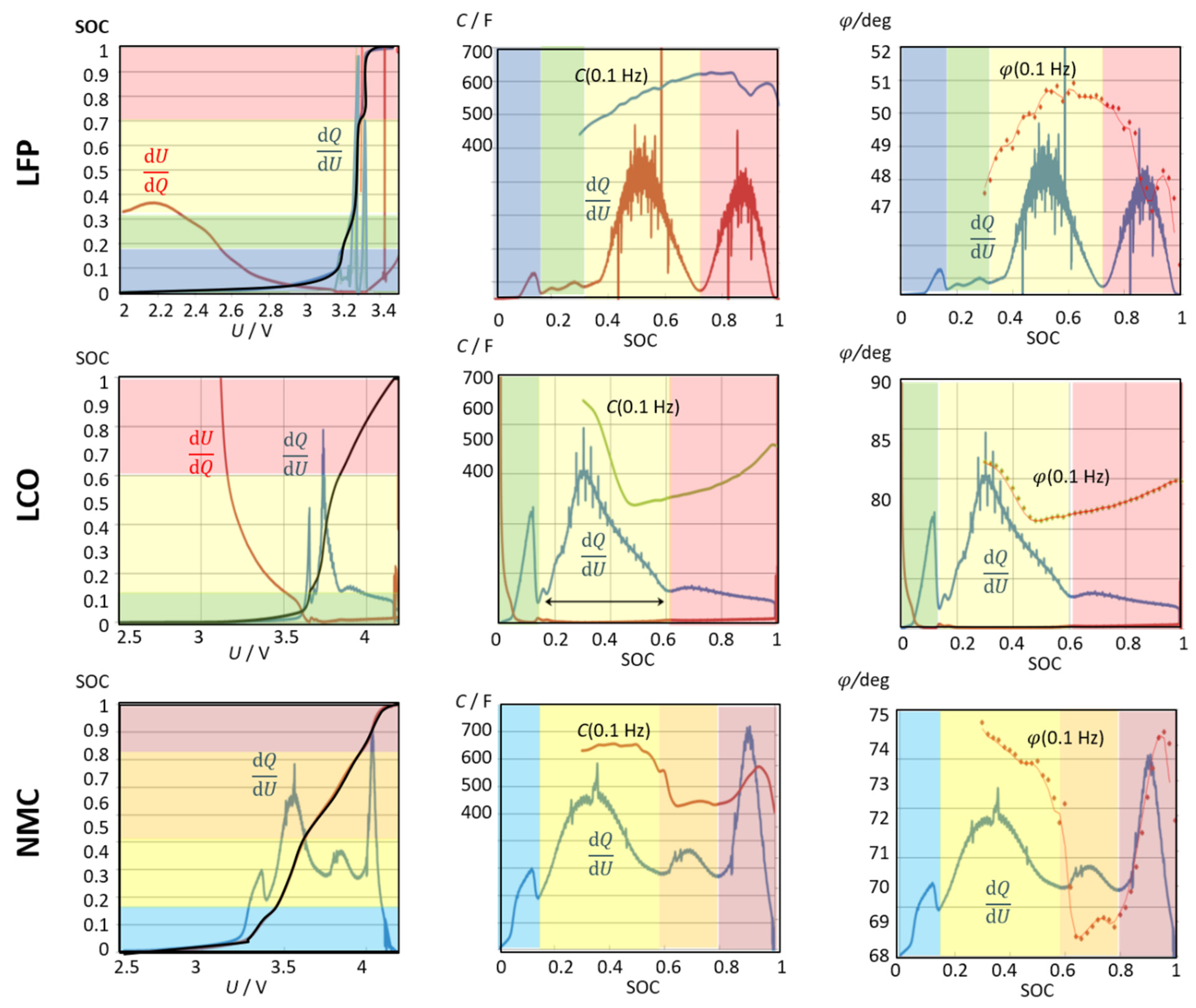
• SOC(U) has an inflection point in the step-shaped curve,
• the resistive quantity dU/dQ is minimum. A steep increase of dU/dQ indicates overcharge and deep discharge, where the differential capacity is small.

On the SOC scale, dQ/dU peaks occur where:

• U(SOC) or U(Q) is flat, i.e., U = constant,
• pseudocapacitance C_S(0.1 Hz) = [−ω Im Z]⁻¹ is almost constant,
• the phase angle φ(0.1 Hz) reaches a maximum or minimum,
• the resistive quantity dU/dQ is minimum.

Figure 10 demonstrates that the capacitance from impedance spectra and the differential capacitance from discharge curves complement each other qualitatively. The maximum pseudocapacitance C(ω) appears close to the peak values of dQ/dU. Since the capacitance depends on the phase angle, dQ/dU peaks are accompanied by phase jumps.

$$\tan \phi \left(\omega \right)=\frac{\mathrm{Im} \underset{\_}{Z}}{\mathrm{Re} \underset{\_}{Z}}=\frac{-1}{\omega C \mathrm{Re} \underset{\_}{Z}}$$

(14)

5.5. Statistical Evaluation of Impedance Spectra

Partial least squares regression (PLSR) [32] is a robust and powerful multilinear regression method in analytical chemistry. Robust means that the model parameters do not change very much when new calibration samples are taken from the total data set. Thus, PLSR is a good alternative to multiple linear regression and principal component regression methods.

(a)

Mathematical background of the method

Multiple linear regression describes every dependent value y (for n samples), by the mean-centered and variance-scaled values x (with m independent variables) and the residual value (error) e.

$$\begin{array}{cc}{y}_i=b_{1i}{x}_{1i}+\cdots b_{mi}{x}_{mi}+e_i& (\mathrm{one} \mathrm{observable} y\mathrm{from} m \mathrm{variables}, \mathrm{one} \mathrm{sample} i)\\ \overrightarrow{y}=\mathit{X} \overrightarrow{b}+\overrightarrow{e}& (\mathrm{one} \mathrm{observable} y \mathrm{and} n \mathrm{samples})\\ \mathit{Y}=\mathit{X} \mathit{B}+\mathit{E}& (n \mathrm{observables} y \mathrm{for} n \mathrm{samples})\end{array}$$

(15)

When solving Equation (15), matrix inversion can cause problems (if m ≤ n) or there is no unique solution (m > n). Therefore, principal component analysis (PCA, Nipals method) recommends writing the data matrix X as the sum of the outer products of two vectors: X = score $\overrightarrow{t}$ loading $\overrightarrow{p}$^T.

In the score matrix T = X P, dimensions having small eigenvalues are excluded. Thus, the multiple linear regression problem can be rewritten: $\mathit{Y}=\mathit{T} \mathit{B}+\mathit{E}$. This regression to the orthogonal data set T of principal components gives no matrix inversion problems.

$$\begin{array}{c}\mathit{X}\left(n,m\right)=\mathit{T}\left(n,a\right)\cdot \mathit{P}{\left(a,m\right)}^{\mathrm{T}}+\mathit{E}\left(n,m\right)={{\displaystyle \sum }}^{ }\overrightarrow{t_h}\cdot {\left(\overrightarrow{p_h}\right)}^{\mathrm{T}}+\mathit{E}\\ \mathit{Y}\left(n,p\right)=\mathit{U}\left(n,a\right)\cdot \mathit{Q}{\left(a,p\right)}^{\mathrm{T}}+\mathit{F}\left(n,p\right)={{\displaystyle \sum }}^{ }\overrightarrow{u_h}\cdot {\left(\overrightarrow{q_h}\right)}^{\mathrm{T}}+\mathit{F}=\mathit{T} \mathit{B} {\mathit{Q}}^{\mathrm{T}}+\mathit{F}\end{array}$$

(16)

The PLSR is, in a simplified way, a double principal component analysis, where the decomposition of the matrices takes place by inclusion of each other. The matrices X and Y are in outer relation, where weighted quantities are necessary for the matrix T. An inner relation describes the proportionality b_h of the h-th column vector of the matrix T to that of the matrix U, ${\overrightarrow{u}}_h=b_h{\overrightarrow{t}}_h$. Herein, b_h are the regression coefficients. In the mixed relation Y = T B Q^T + F, the length $\left|\right|\mathit{F}\left|\right|$ is to be minimized. In order to obtain orthogonal X scores, weights must be introduced.

The algorithm is explained in Geladi et al. [32]. For computation, T and U are the principal component matrices, P and Q are charge matrices, and E and F are reaction matrices of residual values that cannot be explained by principal components. B contains the regression coefficients.

(b)

Numerical implementation

In the calibration or training phase, a model Y = f(X) is searched for by calculating a set of model parameters (regression coefficients). In the prediction or test step, the model is checked by comparing the calculated Y values of further samples with the known values. The mathematical work is easily done by a PHYTON function that uses the base class PLSRegression of the scikit learn or sklearn package [33,34,35]. The pls.fit procedure creates the training function for the model

pls = PLS_opt ()

pls.fit (X, Y, cross_val_opt = True, cval_param = 10)

Y_calc = pls.predict (X’)

where X[n,m] is the data set of n samples with m properties (real numbers, type float)

and Y[n,m] is the data set of m observables for the n samples.

cross_val_opt (boolean): and Cval_param = 10 (integer) say, that a “leave 10 out” cross-validation shall be executed. “Leave one out” cross-validation involves removing value after value from the calibration and computing the model for the reduced data set.

pls.predict is the calculated result for a test data set X’.

(c)

Application example

A Panasonic 18,650 LCO battery was evaluated during 1028 cycles of DOD 20 lifetime testing. The impedance spectra, 24 frequencies from 1 kHz to 0.1 Hz at 26 SOC states from 100% to 50%, as shown in Figure 11, were analyzed with respect to all measured resistance, reactance, and capacitance values. The real part of the impedance was corrected by the electrolyte resistance to normalize the impedance data (Equation (10)).

The m columns of the object matrix X contain electrolyte resistance R_e, corrected real part R(ω), imaginary part X(ω), and pseudocapacitance C(ω), (Equation (9)) for all frequencies ω of the impedance spectrum at all n measurements (lines). The known target values Y are the numbers of charge/discharge cycles of the aging study.

By k-fold cross validation, automatic feature, and component selection was optimized with respect to the squared residual sum (Q²-value), which represents the prediction power of the model.

The cross-validated R²-value is the fit quality of the model.

$$R^2=1-{\frac{{{\displaystyle \sum }}_{i=1}^n\left(y_i-y_{\mathrm{calc},i}\right)2}{{{\displaystyle \sum }}_{i=1}^n\left(y_i-\overline{y}\right)2}}^2$$

(17)

For optimization, we used a heuristic algorithm from the pygmo package. Because not all principal components and frequencies of the impedance spectrum contribute to the prediction, and also contain background noise, the prediction accuracy can be improved by omitting components of little relevance. “Leave one out” cross-validation is useful. The prediction values of the used values and the unused test data result in a modified R² value for the test data, which should be as small as possible.

As a result, our model reaches a good prediction quality (R² = 0.9995, Q² = 0.9979) for the given battery type. Aging changes the charge transfer arc, while the impedance at high frequencies is less affected. The mass transport arc was not evaluated because too long measurement times were required below 0.1 Hz. Interestingly, the varying SOC has no great influence on the PLSR model.

For model validation, a Li-ion battery of the same type after 179 cycles was used. The mean error for all different SoC was 4.9 ± 1.5 cycles (2.72 ± 0.83%). This model can be used for this specific type of battery. For an advanced general aging model, we have to collect more data from different batteries.

5.6. How Fixed Frequency Capacitance Works for SOC Monitoring

So much mathematics! Is there a single impedance value that reflects the actual state of charge? Compared to fitting the CPE element in complete impedance spectra, the capacitance calculated at a certain frequency is simple and does not require any specific model for SOC control. Indeed, for all battery chemistries, pseudocapacitance at medium frequencies reflects the state-of-charge in the correct order of magnitude [6]. Although. the C(SOC) function is not perfectly linear, a third-order polynomial can be fitted from SOC = 60% to 100% (see Supplementary Materials).

Where is the best frequency for the SOC control? In Figure 12, the real part of complex capacitance C(ω) = Re Y/ω (Equation (9)) is shown for its best correlation to the SOC for frequencies between 0.1 Hz and 1 kHz.

There is clearly a statistically significant correlation between C(10 Hz) and the available state-of-charge state of a given battery from new condition to failure.

This means: The relative change of pseudocapacitance C(10 Hz) is suitable as an approximate value for charge control of the same battery, unless the absolute SOC and SOH values are sought. This result confirms that the charge-transfer arc of the impedance spectrum around 10 Hz correctly represents the actual state of charge of a lithium-ion battery during cycle aging. There is no need to measure down to very low frequencies.

6. Summary and Conclusions

The above work can be summarized by the following conclusions.

6.1. Differential Capacity

• Differential capacity C = dQ/dU (capacitance) from charge–discharge curves can be calculated as inverse differential voltage (dU/dQ)⁻¹, avoiding numerical problems.
• Cyclic voltammetry (potentiodynamic) and constant-current discharge (galvanostatic) may be directly compared on the voltage scale.
• The dQ/dU peaks occur where the U(Q) curve is flat (phase equilibrium: ΔU → 0) and the dU/dQ peaks show the steepest decent (phase changes: overcharge, deep discharge).
• The actual state-of-charge SOC(t) = Q(t)/Q₀ (related to the last full charge Q₀) and the actual state-of-health (SOH) are not clearly related to differential capacity. However, the peaks of differential voltage dU/dQ occur at “almost empty” and “almost full”.
• The criterion dQ/dU = dU/dQ = 1 defines the voltage window between practically fully charged (and overcharge is imminent) or practically discharged (and deep discharge is upcoming). The voltage window ΔU between the intersection points correlates with the SOH, but a simple formula SOH(ΔU) cannot be given at the moment.

6.2. Pseudocapacitance Indicates SOC

• Pseudocapacitance is suitable for high and medium charge states without model assumptions in advance. SOC monitoring using capacitance is less sensitive than Ah counting.
• C(SOC) is linear as long as the slope of the discharge curve ΔU/ΔSOC does not change. SOC detection works best for flat U(Q) curves, which is true for LFP batteries. For some lithium ion chemistries, the correlation below 50% SOC is unclear.
• Capacitance (slope of the Q(U) curve) is small and resistance (slope of the U(Q) curve) is great when the battery is depleted or overcharged.

$$\frac{\partial S\mathrm{OC}}{\partial U}=\frac{\mathrm{d}\left(Q/Q_0\right)}{\mathrm{d}U}=\frac{\mathrm{d}\left(CU/Q_0\right)}{\mathrm{d}U}=\frac{C}{Q_0}=\frac{I}{Q_0\frac{\mathrm{d}U}{\mathrm{d}t}}\sim \frac{1}{\left|\underset{\_}{Z}\right| Q_0}$$

(18)

• With increasing temperature, the Nyquist diagram shifts to the left (lower electrolyte resistance), and the semicircle diameter becomes narrower (improved kinetics).

So far, there is no general formula that is able to display and predict the state-of-charge and state-of-health of a battery in all system states over the entire service life. In this work, the criterion of equal differential capacity and differential voltage (dSOC/dU = dU/dSOC = 1) is proposed for the automatic evaluation of the instantaneous charge–discharge curve, whether a battery is full, empty, or about to be overcharged or deep discharged. Further investigation is required to properly address steps in the voltage–charge curve and overcharge effects

References

1. Han, X.; Lu, L.; Zheng, Y.; Feng, X.; Li, Z.; Li, J.; Ouyang, M. A review on the key issues of the lithium ion battery degradation among the whole life cycle. eTransportation 2019, 1, 100005. [Google Scholar] [CrossRef]
2. Li, Y.; Liu, K.; Foley, A.M.; Zülke, A.; Berecibar, M.; Nanini-Maury, E.; Van Mierlo, J.; Hoster, H.E. Data-driven health estimation and lifetime prediction of lithium-ion batteries: A review. Renew. Sustain. Energy Rev. 2019, 113, 109254. [Google Scholar] [CrossRef]
3. Jiang, X.; Chen, Y.; Meng, X.; Cao, W.; Liu, C.; Huang, Q.; Naik, N.; Murugadoss, V.; Huang, M.; Guo, Z. The impact of electrode with carbon materials on safety performance of lithium-ion batteries: A review. Carbon 2022, 191, 448–470. [Google Scholar] [CrossRef]
4. Sanad, M.M.S.; Toghan, A. Chemical activation of nanocrystalline LiNbO3 anode for improved storage capacity in lithium-ion batteries. Surf. Interfaces 2021, 27, 101550. [Google Scholar] [CrossRef]
5. Moustafa, M.G.; Sanad, M.M.S. Green fabrication of ZnAl2O4-coated LiFePO4 nanoparticles for enhanced electrochemical performance in Li-ion batteries. J. Alloys Compd. 2022, 903, 163910. [Google Scholar] [CrossRef]
6. Kurzweil, P.; Scheuerpflug, W. State-of-charge monitoring and battery diagnosis of different lithium-ion chemistries using impedance spectroscopy. Batteries 2021, 7, 17. [Google Scholar] [CrossRef]
7. Kurzweil, P.; Scheuerpflug, W. State-of-Charge Monitoring and Battery Diagnosis of NiCd Cells Using Impedance Spectroscopy. Batteries 2020, 6, 4. [Google Scholar] [CrossRef] [Green Version]
8. Kurzweil, P.; Shamonin, M. State-of-Charge Monitoring by Impedance Spectroscopy during Long-Term Self-Discharge of Supercapacitors and Lithium-Ion Batteries. Batteries 2018, 4, 35. [Google Scholar] [CrossRef] [Green Version]
9. Kurzweil, P.; Schottenbauer, J.; Schell, C. Past, present and future of electrochemical capacitors: Pseudo-capacitance, aging mechanisms and service life estimation. J. Energy Storage 2021, 35, 102311. [Google Scholar] [CrossRef]
10. Kurzweil, P.; Fischle, H.J. A new monitoring method for electrochemical aggregates by impedance spectroscopy. J. Power Sources 2004, 127, 331–340. [Google Scholar] [CrossRef]
11. Kurzweil, P.; Ober, J.; Wabner, D.W. Method for Correction and Analysis of Impedance Spectra. Electrochim. Acta 1989, 34, 1179–1185. [Google Scholar] [CrossRef]
12. Piller, S.; Perrin, M.; Jossen, A. Methods for state-of-charge determination and their applications. J. Power Sources 2001, 96, 113–120. [Google Scholar] [CrossRef]
13. Gauthier, R.; Luscombe, A.; Bond, T.; Bauer, M.; Johnson, M.; Harlow, J.; Louli, A.J.; Dahn, J.R. How do Depth of Discharge, C-rate and Calendar Age Affect Capacity Retention, Impedance Growth, the Electrodes, and the Electrolyte in Li-Ion Cells? J. Electrochem. Soc. 2022, 169, 020518. [Google Scholar] [CrossRef]
14. Waag, W.; Sauer, D.U. State-of-Charge/Health. In Encyclopedia of Electrochemical Power Sources; Garche, J., Dyer, C., Moseley, P., Ogumi, Z., Rand, D., Scrosati, B., Eds.; Elsevier: Amsterdam, The Netherlands, 2009; Volume 4, pp. 793–804. [Google Scholar]
15. Bloom, I.; Christophersen, J.; Gering, K. Differential voltage analyses of high-power lithium-ion cells, 2. Applications. J. Power Sources 2005, 139, 304–313. [Google Scholar] [CrossRef]
16. Dubarry, M.; Svoboda, V.; Hwu, R.; Liaw, B.Y. Incremental capacity analysis and close-to-equilibrium OCV measurements to quantify capacity fade in commercial rechargeable lithium batteries. Electrochem. Solid State Lett. 2006, 9, A454. [Google Scholar] [CrossRef]
17. Grahame, D.C. Properties of the Electrical Double Layer at a Mercury Surface. I. Methods of Measurement and Interpretation of Results. J. Am. Chem. Soc. 1941, 63, 1207–1215. [Google Scholar] [CrossRef]
18. Hamann, C.H.; Hamnett, A.; Vielstich, W. Electrochemistry; Wiley-VCH: Weinheim, Germany, 2007. [Google Scholar]
19. Bard, A.J.; Faulkner, L.R. Electrochemical Methods; Wiley: New York, NY, USA, 2001; Sections 6.2.4 and 14.3.4. [Google Scholar]
20. Barsoukov, E.; Macdonald, J.R. Impedance Spectroscopy: Theory, Experiment, and Applications; Wiley: Hoboken, NJ, USA, 2018. [Google Scholar]
21. Rodrigues, S.; Munichandraiah, N.; Shukla, A.K. A review of state-of-charge indication of batteries by means of a.c. impedance measurements. J. Power Sources 2000, 87, 12–20. [Google Scholar] [CrossRef]
22. Osaka, T.; Mukoyama, D.; Nara, H. Review—Development of Diagnostic Process for Commercially Available Batteries, Especially Lithium Ion Battery, by Electrochemical Impedance Spectroscopy. J. Electrochem. Soc. 2015, 162, A2529. [Google Scholar] [CrossRef]
23. Srinivasan, R.; Demirev, P.A.; Carkhuff, B.G. Rapid monitoring of impedance phase shifts in lithium-ion batteries for hazard prevention. J. Power Sources 2018, 405, 30–36. [Google Scholar] [CrossRef]
24. Birkl, C.R.; Roberts, M.R.; McTurk, E.; Bruce, P.G.; Howey, D.A. Degradation diagnostics for lithium ion cells. J. Power Sources 2017, 341, 373–386. [Google Scholar] [CrossRef]
25. Krupp, A.; Ferg, E.; Schuldt, F.; Derendorf, K.; Agert, C. Incremental capacity analysis as a state of health estimation method for lithium-ion battery modules with series-connected cells. Batteries 2021, 7, 2. [Google Scholar] [CrossRef]
26. Aurbach, D.; Moshkovich, M.; Cohen, Y.; Schechter, A. The study of surface film formation on noble-metal electrodes in alkyl carbonates/Li salt solutions, using simultaneous in situ AFM, EQCM, FTIR, and EIS. Langmuir 1999, 15, 2947–2960. [Google Scholar] [CrossRef]
27. Dedryvere, R.; Foix, D.; Franger, S.; Patoux, S.; Daniel, L.; Gonbeau, D. Electrode/electrolyte interface reactivity in high-voltage spinel LiNi0.5Mn1.6O4/Li4Ti5O12 lithium-ion battery. J. Phys. Chem. C 2010, 114, 10999–11008. [Google Scholar] [CrossRef]
28. Jehnichen, P.; Wedlich, K.; Korte, C. Degradation of high-voltage cathodes for advanced lithium-ion batteries—Differential capacity study on differently balanced cells. Sci. Technol. Adv. Mater. 2019, 20, 1–9. [Google Scholar] [CrossRef] [Green Version]
29. Honkura, K.; Horiba, T. Study of the deterioration mechanism of LiCoO2/graphite cells in charge/discharge cycles using the discharge curve analysis. J. Power Sources 2014, 264, 140–146. [Google Scholar] [CrossRef]
30. La Rue, A.; Weddle, P.J.; Ma, M.; Hendricks, C.; Kee, R.J.; Vincent, T.L. State-of-Charge Estimation of LiFePO4–Li4Ti5O12 Batteries using History-Dependent Complex-Impedance. J. Electrochem. Soc. 2019, 166, A404. [Google Scholar]
31. Ungurean, L.; Cârstoiu, G.; Micea, M.V.; Groza, V. Battery state of health estimation: A structured review of models, methods and commercial devices. Int. J. Energy Res. 2017, 41, 151–181. [Google Scholar] [CrossRef]
32. Geladi, P.; Kowalski, B.R. Partial least-squares regression: A tutorial. Anal. Chim. Acta 1986, 185, 1–17. [Google Scholar] [CrossRef]
33. Pedregosa, F.; Varoquaux, G.; Gramfort, A.; Michel, V.; Thirion, B.; Grisel, O.; Blondel, M.; Prettenhofer, P.; Weiss, R.; Dubourg, V.; et al. Scikit-learn: Machine Learning in Python. J. Mach. Learn. Res. 2011, 12, 2825–2830. [Google Scholar]
34. Consonni, V.; Ballabio, D.; Todeschini, R. Comments on the Definition of the Q2 Parameter for QSAR Validation. J. Chem. Inf. Model. 2009, 49, 1669–1678. [Google Scholar] [CrossRef]
35. Biscani, F.; Izzo, D. A parallel global multiobjective framework for optimization: Pagmo. J. Open Source Softw. 2020, 5, 2338. [Google Scholar] [CrossRef]
Figure 1. Cycle aging of lithium-ion batteries: Loss of available capacity. Full charge–discharge cycles (DOD 100%, solid ––). Partial discharge (DOD 20%, where n = 1 is 5 cycles, dashed - - -).
Energies 15 04520 g001
Figure 2. General procedure for the evaluation of long-term measurements: (a) A single charge–discharge cycle of a LiFePO4 battery, (b) calculated differential capacity dQ/dU, (c) state-of-health and coulombic efficiency η as a function of cycle life. Sections ①②③ correspond to each other.
Energies 15 04520 g002
Figure 3. Used Sanyo-Panasonic LCO battery (UR18650F, 2.3 Ah) after cycle test (SOH = 87%). (a) Constant current charge–discharge characteristics: U cell voltage, I current. (b) Differential capacity dQ/dU and its reciprocal dU/dQ. Data as measured and smoothed (––). The charge/discharge peak dQ/dU near 3.75 V decreases with aging.
Energies 15 04520 g003
Figure 4. Used lithium-ion battery (Panasonic NCR18500A). (a) Constant current charge–discharge characteristics: U cell voltage, I current. (b) Discharge: differential capacity dQ/dU against cell voltage and depth-of-discharge and its reciprocal dU/dQ. Sections ①②③ correspond to each other.
Energies 15 04520 g004
Figure 5. Cyclic voltammogram of a platinum electrode (red) in sulfuric acid against a silver–silver chloride reference electrode (red: differential capacitance C = I/v, scan rate v = 250 mV/s) compared to dQ/dU from constant current charge–discharge curve (blue: cut-off current at 1.35 V and −0.2 V).
Energies 15 04520 g005
Figure 6. (a) Charge–discharge characteristics of different lithium-ion battery cell chemistries; cell voltage U, current I, and temperature change ΔT versus time t. (b) Differential capacity dQ/dU as a function of state-of-charge (SOC = Q/Q0) and depth-of-discharge (DOD = 1−Q/Q0). (c): Differential capacity, dQ/dU = I (dU/dt)−1, as a function of cell voltage U (voltage change dU/dt) for constant current charge and discharge (I = constant). The redox peaks mainly show the lithiated and delithiated metal oxide cathode (+) against the lithiated graphite anode (−). Redox processes: ①②③ Co2+→ Co3+ → Co4+ (3.5–4 V, e.g., Li0.93CoO2 → Li0.73CoO2 → Li0.5CoO2), ④ Ni2+→ Ni3+ → Ni4+ (3.8–4.2 V), ⑤ Mn2+→ Mn3+ → Mn4+ (3.5–3.7 V, e.g., LiMn2O4 → Li0.2Mn2O4), ⑥ Fe2+→ Fe3+ (3.2–3.5 V).
Energies 15 04520 g006
Figure 7. Constant current overcharge of different lithium-ion batteries: (a) cell voltage U, current I, temperature change ΔT with time t. (b) Rise of differential capacity as a criterion for full charge (SOC = 1) and failure by overcharging (SOC > 1 for U ≫ 4 V). The red arrows qualitatively show the lower peak height due to the loss of active material (aging time t) and the peak shift due to the rising cell resistance R.—Panasonic NCR18500A (LiNiCoAl), —Sony US14500VR2B (LiMn2O4), —IFR 18,500 (LiFePO4).
Energies 15 04520 g007
Figure 8. LFP lithium-ion battery (Lithiumwerks) at different temperatures: (a) constant current discharge, (b) relative change of differential capacity dQ/dU against voltage, (c) against state-of-charge. ① almost empty, ② half-full, ③ almost full.
Energies 15 04520 g008
Figure 9. Frequency response of a lithium-ion battery (Panasonic 18650, LCO chemistry) during aging in a DOD 20 cycle test: (a) Nyquist plot: different SOC at the same SOH = 495 cycles in mathematical concentration, (b) equivalent circuit, (c) reactance, (d) resistance, and (e) capacitance at the mean minimum ω m ¯ of the charge-transfer semicircle ③ in the complex plane (1 kHz … 1 Hz). For comparison: a failure device of the same type from a DOD 100 test. (f) Nonlinear least squares fit results with respect to the equivalent circuit: R ohmic resistance, Z = (jω)nC is a constant phase element (lossy capacitance).
Energies 15 04520 g009
Figure 10. Combination of impedance measurement (capacitance C, phase angle φ) and constant current discharge (differential capacity dQ/dU) for different cell chemistries. LFP = LiFePO4 (Lithiumwerks), LCO = (Sanyo-Panasonic), NMC = LG HE.
Energies 15 04520 g010
Figure 11. (a) Multilinear regression model. (b) Impedance spectra of a Sanyo/Panasonic 18,650 cell (LCO chemistry) during cycle aging (DOD 100%), mathematical convention. Thick lines: SOC 100%. Thin lines: SOC 95%, 90%, …, 30%. (c) Calculated cycles with PLSR model against real cycles. Red: Prediction for a different test sample (179 cycles) of the same battery chemistry and type.
Energies 15 04520 g011
Figure 12. Cycle aging of an LCO battery (Panasonic UR18650 FK). (a) Linear correlation of pseudocapacitance from impedance spectra at the best frequency between 1 Hz and 100 Hz. (b) The coefficient of regression (fit quality) between capacitance and SOC is best around 10 Hz (see arrow). Here: SOC = actual state-of-charge of the aged battery with reference to the previous full charge.
Energies 15 04520 g012