
Normalized-Model Reference System for Parameter Estimation of Induction Motors
by
 , , and
Adolfo Véliz-Tejo
1, 
Juan Carlos Travieso-Torres
2,* ,
,
Andrés A. Peters
3,
Andrés Mora
1 and
and
Felipe Leiva-Silva
2 1
Department of Electrical Engineering, Universidad Técnica Federico Santa María, Santiago 8940572, Chile
2
Department of Industrial Technologies, University of Santiago de Chile, Santiago 9170125, Chile
3
Faculty of Engineering and Sciences, Universidad Adolfo Ibáñez, Santiago 7941169, Chile
*
Author to whom correspondence should be addressed.
Energies 2022, 15(13), 4542; https://0-doi-org.brum.beds.ac.uk/10.3390/en15134542
Submission received: 23 May 2022
/
Revised: 6 June 2022
/
Accepted: 17 June 2022
/
Published: 21 June 2022
(This article belongs to the Special Issue Design and Control of Electrical Motor Drives II)
Abstract
:This manuscript proposes a short tuning march algorithm to estimate induction motors (IM) electrical and mechanical parameters. It has two main novel proposals. First, it starts by presenting a normalized-model reference adaptive system (N-MRAS) that extends a recently proposed normalized model reference adaptive controller for parameter estimation of higher-order nonlinear systems, adding filtering. Second, it proposes persistent exciting (PE) rules for the input amplitude. This N-MRAS normalizes the information vector and identification adaptive law gains for a more straightforward tuning method, avoiding trial and error. Later, two N-MRAS designs consider estimating IM electrical and mechanical parameters. Finally, the proposed algorithm considers starting with a V/f speed control strategy, applying a persistently exciting voltage and frequency, and applying the two designed N-MRAS. Test bench experiments validate the efficacy of the proposed algorithm for a 10 HP IM.

1. Introduction
Electrical induction motors (IM) have characteristics that make them particularly attractive for commercial and industrial fixed and variable speed applications. Compared to other electric machines, IM have lower costs, and maintenance requirements for the same output power [1].
IM may have an electric or electronic drive. The first type mainly moves loads with fixed-speed operations, including star-delta starting, and even under variable speeds with discrete levels (e.g., pedestal fans). The electric drive uses the nameplate information for its configuration. It does not need knowledge of the motor-load parameters. The electronic drive covers soft starters [2] and variable speed drives following details regarding the motor-load parameters knowledge.
Low-performance applications needing a starting torque of up to 25% of rated motor torque and from 2% to 4% of steady-state rotor speed-accuracy use a soft starter for fixed speed and variable speed drives with a V/f strategy [3,4,5]. The standard V/f strategy [6] and soft starters mainly employ data from the IM nameplate. Also, two improved versions of the high starting torque V/f strategy [6] avoid using the knowledge of the motor-load parameters. These propose using normalized adaptive controllers [7,8] for the starting current after expanding the techniques given in [9,10], respectively. Both controllers require the detailed structure of the IM dynamical model. However, after assuming unknown parameters, the adaptive controllers ensure the starting current trends to the required value despite the estimated adaptive parameters not converging to the actual values.
Beyond soft starters and variable speed drives with a V/f strategy, other electronic drives use more complex feedback controllers to achieve different goals for the particular requirements [11]. These controllers’ tuning depends on the IM parameters knowledge. For instance, high-performance applications, starting with 100% of rated motor torque and with % of steady-state rotor speed accuracy, use a variable speed drive with field-oriented control (FOC) scheme. This control scheme requires knowledge of the motor-load parameters [3,5,12]. Even when using adaptive controllers [13,14,15], FOC schemes still need, at the very least, the IM rotor time constant parameter. Similarly, variable speed drives with a direct torque control (DTC) scheme use the motor-load parameters for tuning purposes [3,5]. Naturally, any rotor speed observer for sensorless DTC and FOC will also require this knowledge [4].
As manufacturers do not usually provide the IM electrical parameters, variable speed drives with FOC or DTC must estimate them [16]. Moreover, beyond variable speed drives, fault detection, diagnosis, and prognosis also require the knowledge of these parameters [17,18]. Furthermore, efficiency estimation for energy savings planning [19] and other techniques for supervising the IM operation conditions [20], benefit from this information. These requirements motivate the development of identification techniques for IM parameters.
In recent years, researchers have analyzed some techniques for parameter estimation of IM, considering some particular cases and the application of different mathematical algorithms. A neural network-based method, trained with manufacturer data, estimates single and double-cage IM electrical parameters in [21] with up to 12% accuracy for a 22 kW IM. In [22], a deep-Q-learning algorithm estimates the IM rotor resistance and mutual inductance, comparing with three other algorithms. The authors of [23] use a finite element-based method to calculate the IM electrical parameters under a wide range of stator current values. These two studies [22,23] show a similar accuracy for IM of 15 kW and 1.5 kW, respectively. The works [21,22,23] are offline algorithms.
A Kalman filtering approach estimates all IM electrical parameters in [24] with up to 13.3% accuracy for a kW IM. It feeds the IM with a voltage-source inverter and applies a persistent exciting (PE) voltage signal. For an overview of online parameter estimation methods for permanent magnet synchronous machines that could also cover IM, please see [25] and the references therein. This last manuscript insists on the need for PE input signal to ensure the proper estimate. Moreover, it describes the model reference adaptive systems (MRAS) as one of the main techniques employed. Shown electrical parameters estimate error typically refers to the percentage of steady-state error between the proposed method and the results from manual tests, like that of DC injection, locked rotor, and no-load from IEEE std 112 [26]. However, proposals include the inverter feeding the IM. In contrast, the base value does not, and the inverter impacts the results, as described in [27,28]. Moreover, algorithms for controlling FOC and DTC [16] are robust under this level of accuracy, similar to those for supervising operating conditions [17,18,19,20].
The books [29,30] describe the basis for MRAS tuned via a positive gain. The work [31] uses a fixed-gain experimentally adjusted via trial and error. At the same time, the particle swarm optimization technique tunes the fixed-gain in [32]. Later, the work [6] proposes a normalized fixed-gain for the adaptive law settings of an adaptive passivity-based controller [9] applied to IM current control. Finally, the proposal in [7] normalizes the information vector of an adaptive passivity-based controller. It regulates IM starting current, with a normalized fixed-gain and a more straightforward adjustment. The work [33] extends these ideas for MRAC applied to IM. However, the control purpose is often achieved without PE, unlike the identification parameter purpose.
The main contribution of this paper is to propose an algorithm for IM electrical and mechanical parameters estimation via a short tuning march. The algorithm controls the speed with a V/f strategy for starting and stopping, considering the addition of revisited PE rules for voltage and frequency signals and applying two proposed N-MRAS. One novelty of this paper is presenting the N-MRAS, facilitating the adaptive estimation adjustment. It expands the standard MRAS described in [30] for higher-order nonlinear systems, normalizing the information vector and adaptive law gains for a more straightforward tuning method. However, the N-MRAS observer deals with an identification error that may vanish due to a simple orthogonality condition between a vector depending on the estimated parameters and the system information vector. To avoid this, we provide a second novelty, which is the proposal of a design procedure for the PE signals amplitude. It gives steps for a particular operation in the light of the persistent excitation theory to ensure parametric convergence of the estimator. Finally, two designed N-MRAS successfully estimated the electrical and mechanical parameters of a 10 HP IM on a test bench.
The remainder of the manuscript is organized as follows: Section 2 summarizes the preliminaries regarding IM models, parameter estimation, filtering and MRAS. Section 3 derives the proposed method for parameter identification of IM. Section 5 contains results obtained with the proposed method in a laboratory test bench which illustrate its effectiveness. We provide concluding remarks in Section 6.
2. Preliminaries
We begin by describing the parameter estimation background used throughout this work. We base our derivations on the following IM complex - and mechanical load models [34]:
Electrical Subsystem
Mechanical Subsystem
where section Main Notation, located after the Conclusions, describes the meaning of all used variables and parameters. It is valid for all the equations throughout the manuscript.
Based on the previous time-domain model (1)–(3), the following sections describes the background of IM parameters estimation.
2.1. Electrical Parameter Estimation Background
We start by providing the background for the electrical parameter estimation studied herein. We begin by considering a constant operation speed, which allows applying the Laplace transform to the electrical subsystem (1) and (2). By substituting the rotor flux into the current and regrouping terms, we obtain the following transfer function [34]:
where is the order of the numerator, and is the order of the denominator of the transfer function (4), with parameters. The transfer function (4) parameters, , , , and have the following definition [34]:
Using the inverse Laplace transform and regrouping terms, the time-domain current satisfies [34]:
where is the unknown IM electrical parameter vector, and is the known IM information vector. Then, [34] describes the following observer to track the wave-form of the current above in (6):
Here, is the estimated IM intermediate electrical parameter vector, and is the filtered IM information vector. Why filtering? To adequately feed the observer, two identical filters depending on the design parameters and are used (see Figure 1). These filters extract the stator current and voltage and their derivatives, avoiding deriving these variables but obtaining these last through integrals.
Finally, observer (7) allows estimating the IM intermediate electrical parameters , and , minimizing the identification error . Later, the IM electrical parameters compute as follows, based on these intermediate estimated coefficients:
Remark 1.
It is important to note that (8) and (9) consider complex signals and parameters hindering its implementation in control platforms. These expressions are adequate to work with real number signals throughout this paper.
The following sections describes the background of IM mechanical parameters estimation.
2.2. Mechanical Parameter Estimation Background
Proceeding similarly to the previous section, but considering the mechanical subsystem (3) and zero load torque , we obtain the following transfer function:
where the numerator order is , and the denominator order of the transfer function (10) is . Hence, we have parameters given by:
Proceeding as before, that is, using the inverse Laplace transform and regrouping terms, we have the following time-domain speed observer:
Here, is the estimated IM intermediate mechanical parameter vector, and is the filtered IM information vector. Again, ref. [34] considers identical filters depending on the design parameters and to extract the electromagnetic torque and rotor speed to feed the mechanical parameters observer (12) (see Figure 2).
The input of the electromagnetic torque filter should use an observer for , which is not a measured variable. Moreover, it depends on an observed electromagnetic flux. These can be open-loop or closed-loop observers, not described in [34].
Finally, the angular rotor speed observer (12) allows for estimating the coefficients and , minimizing the identification error . Then, the mechanical motor parameters compute as follows:
Remark 2.
Please note that the observer (12) assumes a measured angular rotor speed , which becomes an issue for a sensorless speed control scheme. Herein, the Authors extend this theory to sensorless schemes.
Remark 3.
The following section describes the estimation method.
2.3. General Method for Parameter Estimation
Once filtering the variables of the studied systems (6) and (3) and implementing their respective observers (7) and (12), it allows for computing the corresponding identification errors. These last are and , having the form . Putting together all this information in a general form yields:
Here, are the system’s filtered output measurement and its estimate. The unknown system intermediate parameter vector is . The vector is the estimated system intermediate parameter. The filtered information vector is . Appendix A and Appendix B describe the proves for the estimation methods of proposed N-MRAS and existing LSE.
Now, the general parameter estimation method aims to find an estimated , that ensures the identification error tends to zero over time, i.e., . However, for the vector case, it may find a combination of terms that equals zero, i.e., . In other words, the identification error tends to zero, i.e., , but there is not parametric convergence, i.e., .
One way to obtain parametric convergence is by applying a PE input signal to ensure a certain excitation level for the vector . It prevents the condition and forces as the solution to achieve ([29], Chapter 5). The following section describes the characteristics of a PE input signal.
2.3.1. Persistent Excitation
The persistently exciting input signal studied here has the following structure [34]:
which corresponds to the sum of signals of different spectral lines. According to [29]-Chapter 5, (i.e., the least integer greater than or equal to ). On the other hand, ([30], Chapter 6) proposes that should contain at least frequencies (i.e., the least integer greater than or equal to the number of parameters to estimate ).
For the IM electrical subsystem, as and in (4), we have that , according to [29]. Moreover, for a , consistent with [30], matching these two criteria results. For the IM mechanical subsystem (10) we have that with and , according to [29] and, for a , consistent with [30], matching the results again.
Remark 4.
The following subsection describes the MRAS method used for parameter identification.
2.3.2. MRAS for Parameter Identification
MRAS uses the following adaptive law to ensure the identification error from (14) tends to zero over time, i.e., . It applies to systems with unknown constant system parameters or parameters that vary slowly () [30]:
MRAS adjusts its convergence rate through the design parameter , which is a positive definite matrix.
Appendix A describes the theoretical proof of the MRAS for the Paramater identification method.
Remark 5.
The following section proposes an N-MRAS and applies it to the IM parameters estimate, joined to filtering and PE input signals.
3. Proposal
This section proposes a general N-MRAS for linear systems and applies it to IM parameter estimation.
3.1. Proposed N-MRAS
The N-MRAS applies to filtered linear systems modeled by the following Laplace-domain transfer function:
where . Moreover, is the filtered signal of , and is PE. The transfer function (17) may be re-expressed in the time domain as follows:
with and are the n-th and m-th time-derivative of signals and , respectively. Moreover, the system could even be nonlinear and represented as follows:
Theorem 1.
The following normalized model reference adaptive system tracks the output of the nonlinear system (19), i.e., :
while ensuring its adaptive parameter tends to the systems parameter over time, i.e., .
Here, is a normalization matrix, defined as the diagonal matrix of a normalization vector, i.e., . The terms , , , , and , represent the maximum operational range of ,, ,, and , respectively. The design aims obtaining a normalized information vector with a range of 100. Then, the fixed-gain , has the form ([30], Section 5.5), with herein. The term allows a fast tuning for a reasonable operating range and the design parameter allows a fine-tuning adjustment if needed.
Proof.
See Appendix B which describes the theoretical proof of the proposed N-MRAS. □
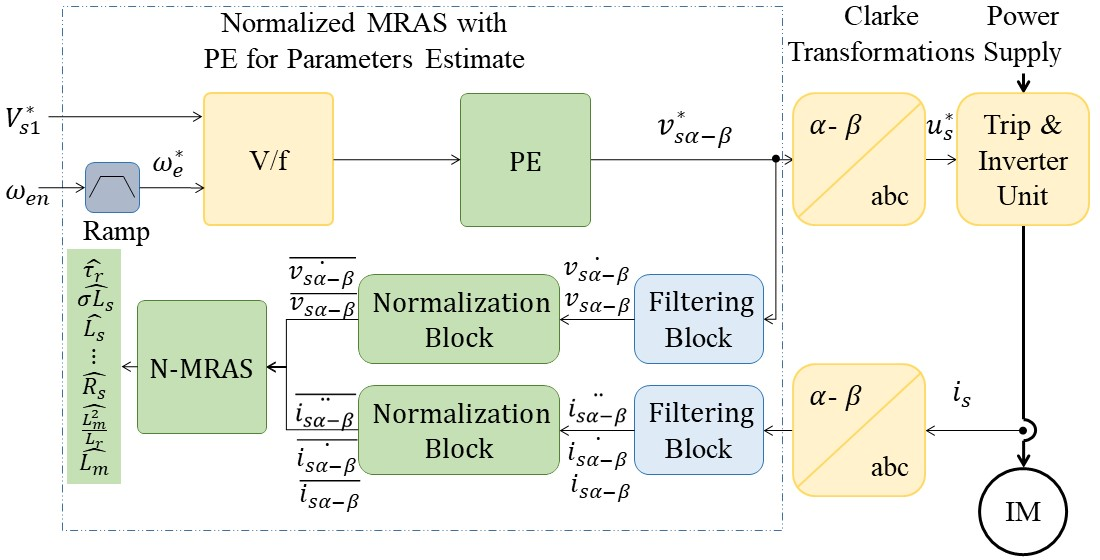
Figure 3 shows the proposed N-MRAS block diagram.
Following there are details of the filtering blocks and supply characteristics.
Remark 6.
The appropriate order of the filter ( or higher) is the one that ensures a lower noise presence in the estimated variable . The design for a real-time software implementation of the analog nth-order butterworth filter for a given cut frequency considers: running the matlab function to obtain the zeros, poles and gain of the filter; later, getting its polynomial representation using to extract its coefficients to ; and finally, obtaining the filter parameters as follows: , , , , …, to have a unitary numerator gain.
Remark 7.
Regarding the PE input signal , it is clear enough that the needed harmonic content has at least frequencies (i.e., the least integer greater than or equal to the number of parameters to estimate ) ([30], Chapter 6). Moreover, herein we propose the following considerations for the signal amplitude:
- 1.
- Make sure that is closer but not beyond the system rated .
- 2.
- Associate a different to a different component
- 3.
- Ensure choosing in such a way that associated component is closer but not beyond the rated component.
The must ideally excite the whole input vector and also the output vector , which depends on the nonlinear system characteristics.
The following section applies these proposals to IM.
3.2. N-MRAS Applied for Sensorless IM Parameter Estimation
Based on this IM dynamical model, the following subsections apply the N-MRAS to IM parameters estimation.
3.2.1. N-MRAS for IM Electrical Parameters Estimate
Here, for the no-load condition . Moreover, after applying to the electrical subsystem a similar procedure to the one used in Section 2, considering a constant operation speed, Laplace transformation, regrouping terms, and using the inverse Laplace transformation, we obtain
Finally, based on the intermediate electrical parameters definitions made explicit in (24), the IM main electrical parameters are obtained as:
These main electrical parameters allow obtaining thee other IM electrical parameters also used by different algorithms as described in the Introduction:
obtained from (33) after assuming [22],
Figure 5 depicts the proposed N-MRAS_e block diagram.
Section 3.2.3 designs the supply characteristics.
The filtering blocks of Figure 5 are the identical filters details in Figure 6 that extract the electrical variables and their derivatives through integral actions. These are two orders higher than the filters decribed in [34], decreasing this way the ripple amplitude of . These are real-time software implementations of analog filters, programmed as part of the algorithm.
The filters design considers a 4th-order () and a cut frequency rad/s. Then the matlab function gives the zeros, poles and gain of the filter. Its polynomial representation, obtained from allows extracting its coefficients to and finally obtaining the filter parameters as follows: , , , , to have a unitary numerator gain.
The following subsection describes the proposed N-MRAS for IM mechanical parameter estimation.
3.2.2. N-MRAS for IM Mechanical Parameter Estimate
Based on the mechanical subsystem (10), the N-MRAS estimator with its intermediate mechanical parameters takes the form:
Then, we use (13) to obtain . Here, the estimator input signals for the no-load condition working at the rated frequency are the angular rotor speed and the electromagnetic torque computed as:
Based on (21) and (22), after assuming , the rotor flux is observed as follows using the previously estimated electrical parameters:
Here, a recursive Kalman filter [36] computes . It considers the covariance matrix of the measurement noise . This last is the average of the covariance of the vector obtained after measuring each phase current for 0.2 s with a turned-off inverter. Moreover the covariance matrix of the process noise , lower than R after considering an accurate model.
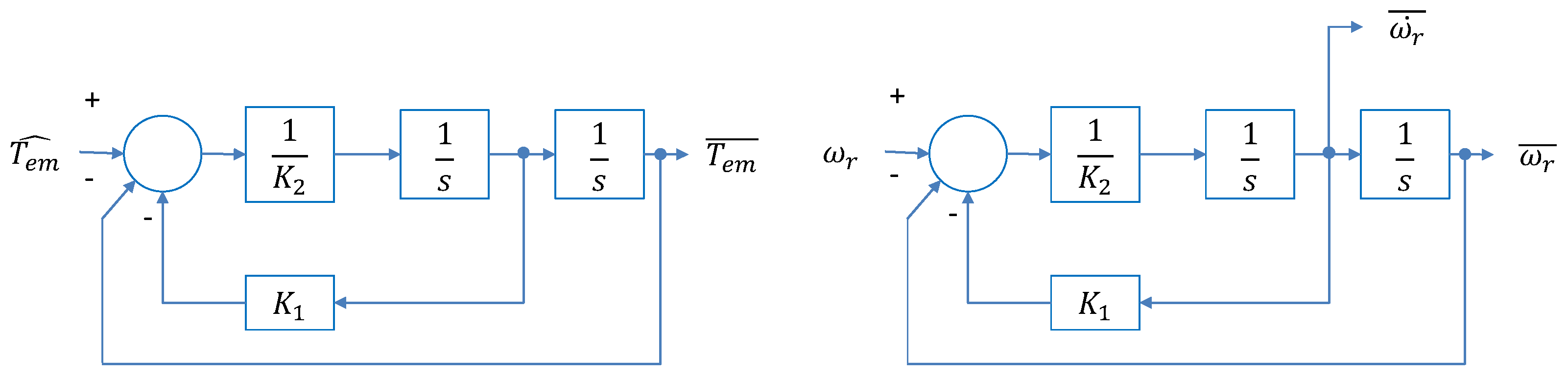
Figure 7 depicts the proposed N-MRAS_e block diagram.
Section 3.2.4 designs the supply characteristics.
Figure 7 uses the filters detailed in Figure 8 to extract the mechanical variables and a derivative through integral actions.
This work uses identical filters for electrical and mechanical variables, with the configuring described in the previous subsection.
The following subsections describe the proposed PE input signals to ensure parametric convergence for the proposed N-MRAS. It uses the nameplate information depicted in Table 1 of the IM existing in our laboratory.
This information allows calculating the rated electrical frequency rad/s, the rated electromagnetic torque Nm, and configuring PE signals as follows.
3.2.3. PE for the Electrical Subsystem
This subsection proposes the PE signal for the electrical subsystem. From (25), we have parameters, hence, our input signal requires over frequencies to be PE [30]. It gives that the required input voltage may have the form
where and are the fundamental voltage and frequency, respectively, with rad/s (50 Hz, please see Table 1). Moreover, and are the amplitudes of the highest and lowest harmonics, respectively.
Given that plant parameters are unknown, it’s impossible to directly establish frequencies to excite the natural modes. Moreover, the inverter nonlinearities make it difficult to modulate low frequencies and voltages [27]. This paper uses harmonic frequencies above the rated frequency of the motor (50 Hz). It also considers the alert of [34] about bad performance estimations with higher frequencies, up to 300 Hz. Herein, 125 Hz ensures the highest stator current consumption under the nominal one. Hence, we choose rad/s (125 Hz), and rad/s (65 Hz).
Regarding the voltage amplitudes, we propose working at the linear modulation limit. Hence, the total voltage amplitudes fulfill the following criteria
Later, we define that excites the voltage derivative and excites the stator current. Moreover, the estimations consider the IM working with no load around the rated angular frequency as a pure inductive load, valid for motors above a certain level of power, around 3.7 kW. For lower power motors, the motor equivalent resistance drop is not negligible. As a result, it yields:
Canceling terms in the second equation, rearranging terms to obtain the voltage amplitudes, and considering the definition from (45), it gives
Here, the lowest harmonic voltage is selected by imposing a ratio with the current produced by the highest harmonic . Furthermore, the latter depends on the ratio , which represents the contribution of the highest harmonic to the temporal variation of the main voltage. Substituting (45), (48), and (49) into (46), and rearranging terms, computes:
This way, ensures that the inverter works in the linear zone limit. The other two ratios are and . The following sections describe the proposed PE input signals for mechanical parametric convergence of the proposed N-MRAS.
3.2.4. PE for the Mechanical Subsystem
This subsection proposes the mechanical subsystem PE input signal. From (38), we have parameters, hence, our input signal requires frequency to be PE [30]. The following input voltage with time-varying electrical frequency ensures the required PE:
Here, after adjusting rad/s (0,5 Hz) for slow mechanical variations, the frequency varies in the interval . For simplicity, we maintain the excitation voltage level with of the rated voltage. The following section described a proposed Algorithm that would allow implementing the proposal and it comparison with the LSE method.
3.3. Proposed Algorithm for Parameters Estimate
Algorithm 1 starts computing initial values of harmonic frequency and voltage amplitudes to assure PE for electrical parameters estimate. Then, it starts with a V/f control strategy with a voltage reduced to the first voltage amplitude. After reaching the nominal speed steady state, it inserts harmonics and the electrical parameters estimation occurs during 180 s. Later, mechanical parameters estimation takes place; and finally, the motor is stopped.
| Algorithm 1 Pseudocode of the Proposed Initial Tuning Parameter Estimate. |
|
Algorithm 1 runs first via simulations in the following section, which depicts and discusses the obtained results before the experimental tests.
4. Simulation Results
Before the experimental testing in a laboratory test bench, simulations evidence the proposal’s effectiveness in a safety environment. For this purpose, Algorithm 1 runs with the N-MRAS_e and N-MRAS_m methods on a modeled experimental setup for 350 s. It uses the test bench Host PC Simulink version 8.9 and Matlab R2017a. It considers a three-phase voltage source inverter feeding an IM of 10 HP with test bench parameters described in Appendix D and a no-load condition. It also uses a pulse width modulation switching frequency of 8 kHz.
The simulation test considers different faulty conditions to verify the N-MRAS effectiveness. It starts with IM configured with its base parameters values from Appendix D. Later, the value increases in ratios in step 1, as in [24], at 150 s. Similarly, the value rises in proportions with step 2 at 250 s.
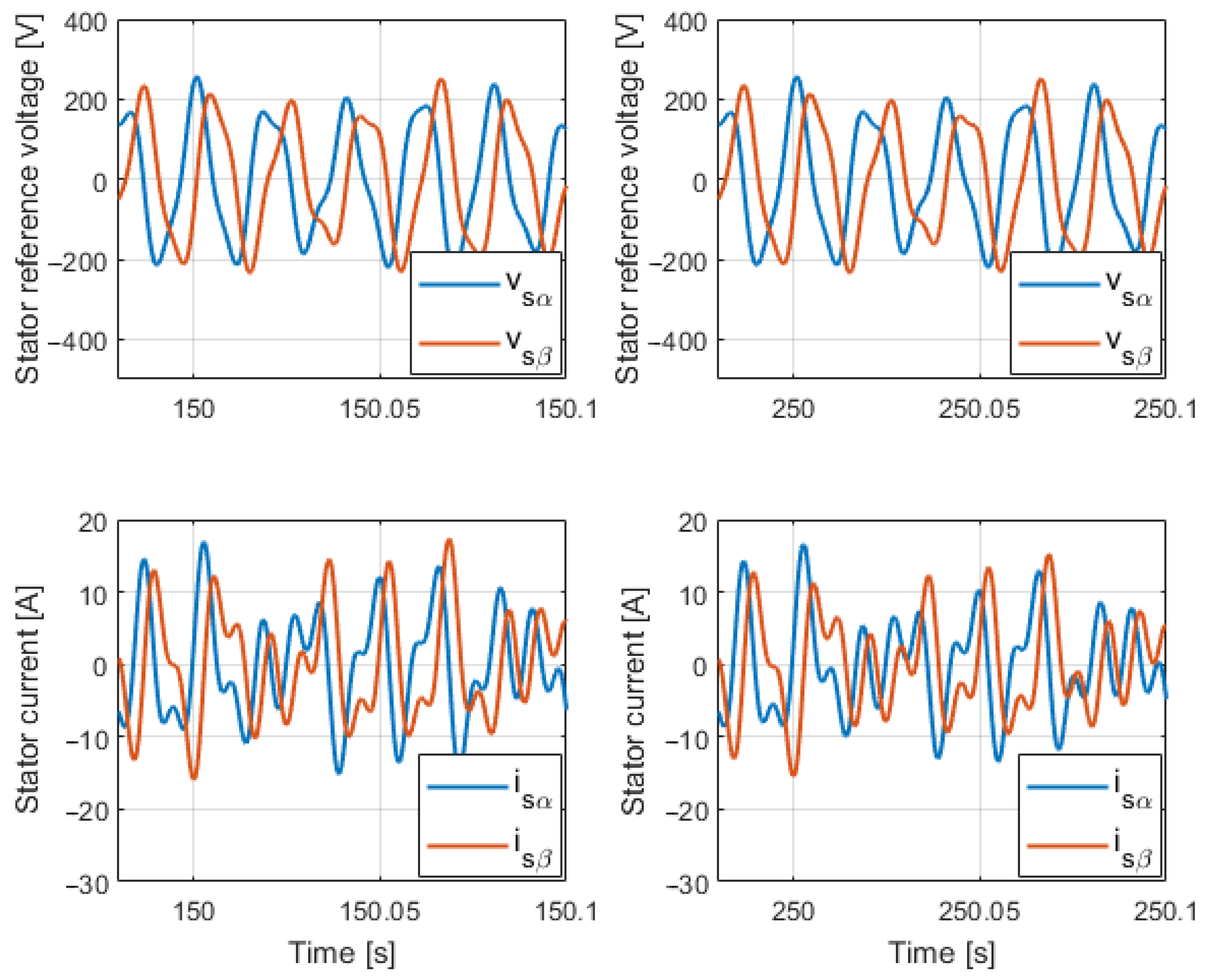
Figure 9 shows the required PE voltage applied and the measured current waveform. These are shown in - coordinates for better appreciation of the excitation level during the parameter estimate. Both signals show a level of excitement. The voltage and current amplitudes are inside the allowed operational range, as designed in Section 3.2.3. The current amplitude slightly decreases at 150 s after the stator resistance increases.
Figure 10 shows the intermediate electrical parameters estimate. All tend to their corresponding base values with different levels of steady-state accuracy. Here, and depict the best results, implying that the applied ensures the required excitement for the stator voltage and its first-time derivative. However, , , and have the less exact values. Hence, a priori, the excitement of the stator current and its first-time derivative seems not to be ideal.
Based on Figure 10 results, the algorithm gives Table 2 results. It uses the following steady-state error expression as a standard practice reported in several IM estimation studies [21,22,23,24].
Table 2 results show that parameters estimate accuracy is lower than 10% in all cases. The estimations are similar before applying the steps that change parameters values than after step 1 and step 2. Thus, the proposed N-MRAS_e method is robust under parameter variations. Moreover, the applied voltage and current amplitudes are inside the allowed operational range verifying a safe operation for the experimental tests.
Next, the mechanical estimate considers that the value increases in ratios in a step way at 250 s. Figure 11 shows the required PE voltage applied and the measured current waveform during the parameter estimate. Moreover, Figure 12 depicts the intermediate mechanical parameters estimate.
Again, both signals show a level of excitement, as displayed in Figure 11. The amplitudes of the voltage and the current are below the rated values, according to the design of Section 3.2.4. The current amplitude slightly increases at 250 s after the motor inertia increases.
Figure 12 shows that the required intermediate mechanical parameter tends to its base value with a high level of steady-state accuracy. It implies that the applied ensured the excitement needed for electromagnetic torque. Please, lets´s keep in mind Remark 3 describing how we only estimate .
Results shown in Table 2 have an inertia accuracy lower than %. The estimation is similar before and after applying the step-change in the parameter value. Thus, the proposed N-MRAS_m method is also robust under parameter variation.
After the obtained simulation results, we conclude that the proposed algorithm tracks the changes in parameter values. Moreover, the applied voltages are PE and will ensure a safe IM operation for the experimental tests described in the following section.
5. Experimental Results
A laboratory test bench was used to experimentally verify the proposal, obtaining comparative results. It is comprised of a real-time simulator controller OPAL-RT 4510 v2, controlling a three-phase voltage source inverter feeding an IM of 10 HP disconnected from the load. It uses a pulse width modulation switching frequency of 8 kHz. Simulink version 8.9 and Matlab R2017a installed on a Host PC allow building the compared strategies, and downloading them to the OPAL-RT using the software RT-LAB v2020.2.2.82. Figure 13 shows the test bench used to validate the proposal.
The following section describes the experimental tests performed to validate the proposed Algorithm including N-MRAS for the 10 HP IM of the existing test bench shown in Figure 13.
5.1. Experimental Tests Performed
This section describes the obtained results for the IM parameter estimation, considering the proposed N-MRAS and the LSE method, applied through the algorithm, versus the standard manual testing.
First, Algorithm 1 runs, obtaining the oscilloscope stator current wave-forms of Figure 14. Figure 14 shows the current curves after starting harmonic insertion for the electrical parameter estimation. Please note that there are current peaks of almost the nominal IM current, but not over it. That is the importance of the proper choice of the harmonic voltage amplitudes. Moreover, the applied PE voltage frequencies ensures a level of excitation of the stator current.
After the electrical parameter estimate, Algorithm 1 starts harmonic insertion for the mechanical parameter estimation. Figure 15 shows the stator current curves. There are no electrical harmonics, and we have a no-load torque condition; thus, the current peak is around . However, please observe the oscillations provoked by the mechanical harmonic insertion after considering the oscillatory frequency signal (51).
The following sections show the obtained comparative experimental results.
5.1.1. Electrical Parameters Estimates Results
The compared methods for estimating the electrical parameters of IM are the following:
IEEE std 112 [26]: Parameters obtained with manual tests of DC injection, locked rotor, and no-load.
N-MRAS_e: Composed of Equations (25)–(28).
SSM_e: Composed of equation (A12).
Figure 16 shows the experimental results obtained with the setup for the IM intermediate electrical parameter estimation. Similar to simulations, all estimated values tend to their corresponding base values with different levels of steady-state accuracy. Here, has the best results, with an applied that ensures the required excitement for the stator voltage first-time derivative. However, , , and have the less exact values. Again, the excitation of the stator current and its first-time derivative seems not to be ideal.
As described in Section 3.2.1, the obtained intermediate parameters illustrated in Figure 16 allow computing of the different electrical parameters defined in the same section. Table 4 summarizes these estimations based on Equations (29) through (37). It is possible to see in Figure 16 that the intermediate estimate through N-MRAS_e converges within approximately 50 s. The zoomed-in part on the right side of Figure 16, highlights that N-MRAS_e produces closer estimates that the ones obtained with LSE_e. Consequently, as shown in Table 4, the magnitude of the errors for the IM electrical parameters estimated with N-MRAS_e are lowest than those achieved with LSE_e. Table 4 shows that parameters estimate accuracy is within other works ranges [21,22,23,24]. A further improvement would be applying a PE voltage signal that compensates for the inverter’s impact described in [27,28].
5.1.2. Mechanical Parameters Estimates Results
The compared methods for estimating the IM mechanical parameters are as follows:
Inertia Testing [37]: Deceleration manual test for inertial identification. There is no data for the parameter.
N-MRAS_m: Integrated by Equations (38), (39), (40) and (41).
SSM_m: Conformed by Equation (A12).
Figure 17 presents the comparative results for the intermediate mechanical parameters estimate. The N-MRAS_m starts estimating the intermediate mechanical parameters for around 30 s, while the LSE_m computes data from the last 5 s ( = 15,000). Figure 17 shows that the required intermediate mechanical parameter tends to its base value with the high level of steady-state accuracy, implying that the applied ensures the excitement needed for electromagnetic torque even with the inverter’s presence.
Both methods, the proposed N-MRAS_m and the existing LSE_m, show similar behavior, although the N-MRAS_m has the highest accuracy of the two.
As discussed in Remark 3, with an unloaded IM, does not characterize the corresponding IM-load viscosity coefficient. Hence, we only estimate . Table 5 shows that N-MRAS_m has the lowest error of compared with the of of LSE_m. Thus, the N-MRAS_m has the highest accuracy for this IM mechanical parameter estimate.
6. Conclusions
This work proposes an N-MRAS for high order nonlinear systems parameter estimation, and simple tuning, normalizing and filtering of the information vector. It injects harmonic signals with a desired frequency and amplitude to ensure persistent excitation and convergence of the adaptive parameters to the system parameters. Moreover, this paper presents some rules to precisely define the amplitude of the injected signal. At the same time, conventional design criteria determine their frequencies. It includes its formal stability proof.
Later, it applies to IM’s electrical and mechanical parameters estimate, which is a challenging application since an inverter feeds the IM and imposes switched voltage wave-forms. Furthermore, IM performance depends on the input voltage and frequency ratio. Considering all these aspects, the authors propose a short tuning march algorithm for motors above 3.7 kW. It works at nominal speed and no-load conditions, allowing for the complete identification of the IM parameters. In essence, it acts as follows:
- -
- It applies a V/f speed control strategy with reduced voltage.
- -
- Administer PE voltage and frequency signals.
- -
- And finally, it runs two N-MRAS, starting with one for the electrical parameters and finalizing with the other for the motor inertia parameters.
Experimental analysis conducted on a test bench with a 10 HP motor validates a proposed algorithm for IM electrical and mechanical parameter estimation. The results were contrasted with standard manual procedures (DC injection, No-load, and blocked rotor test) and the LSE method. It shows satisfactory results with appropriate precision compared to similar work.
The proposed N-MRAS shows to be an alternative to the methods [21,22,23,24], having a more simple tuning. Its results may also provide the IM parameters estimate to algorithms for controlling, like FOC and DTC [16], and those for supervising operating conditions [17,18,19,20].
Future works will explore the application of the proposed method to feed lower power IM. Moreover, further experiments and theoretical developments could improved the obtained accuracy.
Author Contributions
Conceptualization, methodology, writing—original draft preparation, and visualization, A.V.-T. and J.C.T.-T.; investigation, formal analysis, supervision, project administration, data curation, and resources and funding acquisition, J.C.T.-T., A.A.P. and A.M.; validation, software, and writing—review and editing, F.L.-S. All authors have read and agreed to the published version of the manuscript.
Funding
This research was funded by FONDEF Chile, grant ID17I20338; FONDECYT Chile, grant 11221365; and FONDECYT Chile, grant 11190852.
Institutional Review Board Statement
Not applicable.
Informed Consent Statement
Not applicable.
Data Availability Statement
Not applicable.
Conflicts of Interest
The authors declare no conflict of interest.
Abbreviations
The following abbreviations are used in this manuscript:
| IM | Induction motors |
| FOC | Field-oriented control |
| DTC | Direct torque control |
| MRAS | Model reference adaptive system |
| N-MRAS | normalized MRAS |
| DC | Direct Current |
| PE | Persistent Excitation |
| LSE | Lest square Error |
Main Notation
The following main notations are used in this manuscript:
| , , and | Required rotor, actual, and electrical angular speed |
| and | Rated rotor and required angular speed |
| and | Actual and rated angular slip speed |
| Rotor position | |
| stator voltage in - coordinates | |
| stator current in - coordinates | |
| rotor flux in - coordinates | |
| Frequency domain stator voltage in - coordinates | |
| Frequency domain stator current in - coordinates | |
| Frequency domain rotor flux in - coordinates | |
| , and | Electromagnetic, load and rated torque. |
| and | Rated voltage and current per phase (RMS value) |
| DC-link voltage. | |
| Rated electrical frequency in Hz | |
| p | Number of poles |
| and | Stator and rotor resistance |
| and | Stator and rotor leakage inductance |
| , , and | Stator, rotor, and magnetizing inductance |
| Electrical relationship constant | |
| Leakage or coupling coefficient, given by | |
| Stator transient resistance, with | |
| Stator transient time constant. given by | |
| Rotor time constant | |
| D | Mechanical friction factor |
| J | Moment of inertia |
| and | Clarke transformation and its inverse |
Appendix A. Proof of Stability of MRAS for Parameter Identification from Section 2.3.2
Proof.
The error model, composed of the identification error from (14) and the identification adaptive-law (16), has associated the following Lyapunov type energy function and its time derivative (energy variation over time):
The following expression describes the process after substituting the identification adaptive law from (16) into this last expression of the energy variation over time, canceling the terms , and considering the identification error equation (14):
As a result, the energy variation over time (A3) of the Lyapunov type energy function (A1) is less than or equal to zero for any ; thus, the autonomous system is stable, i.e., (the identification and parameters’ errors are bounded). As and are bounded, then is bounded, i.e., .
Moreover, after computing the first-time derivative of the identification error , it equals , where as and are stable, and is bounded, then (the variation over time of the identification error is bounded). Similarly, after computing the first-time derivative of the identification adaptive law , it equals , where as and are stable, and is bounded, then (the variation over time of the first-time derivative of the identification adaptive law is bounded).
Integrating both sides of (A2), we obtain
Here, like we have a bounded energy left-side term, we conclude that the euclidean error norm is bounded, i.e., , then the parameter error euclidean norm is bounded too since , i.e, . Hence, according to Barbalat’s Lemma ([30], Lema 2.12, Corollary 2.9), as (the error tends to zero over time), and as (the parameter error first-time derivative tends to zero over time).
Appendix B. Proof of Stability of Theorem 1
Proof
(Proof of Theorem 1). After subtracting the filtered system model (18) from the identification model given in (20), the estimated output, considering that and , and making some algebraic arrangements, it is obtained as
All parameters are assumed to be unknown and constant, which may have a slow variation. Thus, as we have that its first-time derivative is , due to . Substituting the adaptive law (20) into this last expression, it yields . This last equation joined to the identification error (A4), represents the following autonomous error model:
This error model (A5), has associated the following Lyapunov type energy function and its first-time derivative:
The following expression describes the process after substituting the first-time derivative from (A5) into this last expression, canceling terms and considering the identification error Equation (A5):
The right side of (A7) shows that the first-time derivative of the Lyapunov function (A6) is less than or equal to zero for any ; thus, the autonomous system is stable, i.e., . As and are bounded, then is bounded, i.e., .
Moreover, the first-time derivative of the identification error equals , and as and are stable, and is bounded, then . Similarly, the first-time derivative of the adaptive law equals , and as and are stable, and is bounded, then .
Appendix C. Obtaining Least Squares Method for Parameters Identification
Proof.
We can apply the least squares method to (14), rearranging the error equation, and minimizing the sum of the square errors of measurements [38] we have:
Thus, it takes (A8) and evaluates
which, after considering the vector property where we express . Then, canceling terms, it gives , and yields
Finally, rearranging last equations the parameter estimates follows:
Here, after taking measurements and having a unique set of data, the SSE method computes once as follows:
where the set of the filtered outputs and information matrix are defined as:
□
Appendix D. Manual Testing Results of Parameters Estimate
After following the IEEE std 112 [26] and the Inertia Testing [37], results give the base value electrical and mechanical parameters, respectively, shown in Table A1. Simulations use these parameters for the modeled IM, as well as the experimental results for comparison purposes.

Table A1.
Base Parameters Values Obtained from Manual Testing.
| Parameter | Value |
|---|---|
| [] | |
| [] | |
| [mH] | |
| [mH] | |
| [mH] | |
| [kg m] |
References
- Chapman, S. Electric Machinery Fundamentals; McGraw-Hill Series in Electrical and Computer Engineering; McGraw-Hill: New York, NY, USA, 2012. [Google Scholar]
- Navarro-Navarro, A.; Zamudio-Ramirez, I.; Biot-Monterde, V.; Osornio-Rios, R.A.; Antonino-Daviu, J.A. Current and Stray Flux Combined Analysis for the Automatic Detection of Rotor Faults in Soft-Started Induction Motors. Energies 2022, 15, 2511. [Google Scholar] [CrossRef]
- Vas, P. Electrical Machines and Drives: A Space-Vector Theory Approach; Monographs in Electrical and Electronic Engineering; Clarendon Press: Oxford, UK, 1992. [Google Scholar]
- Vas, P. Sensorless Vector and Direct Torque Control; Monographs in Electrical and Electronic Engineering; Oxford University Press: New York, NY, USA, 1998. [Google Scholar]
- Bose, B. Modern Power Electronics and AC Drives; Eastern Economy Edition; Prentice Hall PTR: Hoboken, NJ, USA, 2002. [Google Scholar]
- Travieso-Torres, J.C.; Vilaragut-Llanes, M.; Costa-Montiel, Á.; Duarte-Mermoud, M.A.; Aguila-Camacho, N.; Contreras-Jara, C.; Álvarez-Gracia, A. New Adaptive High Starting Torque Scalar Control Scheme for Induction Motors Based on Passivity. Energies 2020, 13, 1276. [Google Scholar] [CrossRef] [Green Version]
- Travieso-Torres, J.C.; Contreras-Jara, C.; Diaz, M.; Aguila-Camacho, N.; Duarte-Mermoud, M.A. New Adaptive Starting Scalar Control Scheme for Induction Motor Variable Speed Drives. IEEE Trans. Energy Convers. 2022, 37, 729–736. [Google Scholar] [CrossRef]
- Travieso-Torres, J.C.; Duarte-Mermoud, M.; Díaz, M.; Contreras-Jara, C.; Hernández, F. Closed-Loop Adaptive High-Starting Torque Scalar Control Scheme for induction Motor Variable Speed Drives. Energies 2022, 15, 3489. [Google Scholar] [CrossRef]
- Travieso-Torres, J.C.; Duarte-Mermoud, M.A.; Sepúleveda, D.I. Passivity-based control for stabilization, regulation and tracking purposes of a class of nonlinear systems. Int. J. Adapt. Control. Signal Process. 2007, 21, 582–602. [Google Scholar] [CrossRef]
- Tracking control of cascade systems based on passivity: The non-adaptive and adaptive cases. ISA Trans. 2006, 45, 435–445. [CrossRef] [Green Version]
- Kumar, R.; Das, S.; Syam, P.; Chattopadhyay, A.K. Review on model reference adaptive system for sensorless vector control of induction motor drives. IET Electr. Power Appl. 2015, 9, 496–511. [Google Scholar] [CrossRef]
- Costa, A.; Vilaragut, M.; Travieso-Torres, J.C.; Duarte-Mermoud, M.; Muñoz, J.; Yznaga, I. Matlab based simulation toolbox for the study and design of induction motor FOC speed drives. Comput. Appl. Eng. Educ. 2012, 20, 295–312. [Google Scholar] [CrossRef]
- Duarte-Mermoud, M.; Travieso, J. Control of induction motors: An adaptive passivity MIMO perspective. Int. J. Adapt. Control. Signal Process. 2003, 17, 313–332. [Google Scholar] [CrossRef] [Green Version]
- Two simple and novel SISO controllers for induction motors based on adaptive passivity. ISA Trans. 2008, 47, 60–79. [CrossRef]
- Duarte-Mermoud, M.; Travieso, J.; Pelissier, I.; González, H. Induction Motor Control Based On Adaptive Passivity. Asian J. Control. 2012, 14, 67–84. [Google Scholar] [CrossRef] [Green Version]
- Toliyat, H.; Levi, E.; Raina, M. A review of RFO induction motor parameter estimation techniques. IEEE Trans. Energy Convers. 2003, 18, 271–283. [Google Scholar] [CrossRef]
- Bellini, A.; Filippetti, F.; Tassoni, C.; Capolino, G.A. Advances in Diagnostic Techniques for Induction Machines. IEEE Trans. Ind. Electron. 2008, 55, 4109–4126. [Google Scholar] [CrossRef]
- Da, Y.; Shi, X.; Krishnamurthy, M. Health monitoring, fault diagnosis and failure prognosis techniques for Brushless Permanent Magnet Machines. In Proceedings of the 2011 IEEE Vehicle Power and Propulsion Conference, Chicago, IL, USA, 6–9 September 2011; pp. 1–7. [Google Scholar] [CrossRef]
- Al-Badri, M.; Pillay, P.; Angers, P. A novel technique for in situ efficiency estimation of three-phase IM operating with unbalanced voltages. IEEE Trans. Ind. Appl. 2016, 52, 2843–2855. [Google Scholar] [CrossRef]
- Białoń, T.; Niestrój, R.; Michalak, J.; Pasko, M. Induction Motor PI Observer with Reduced-Order Integrating Unit. Energies 2021, 14, 4906. [Google Scholar] [CrossRef]
- Çetin, O.; Dalcalı, A.; Temurtaş, F. A comparative study on parameters estimation of squirrel cage induction motors using neural networks with unmemorized training. Eng. Sci. Technol. Int. J. 2020, 23, 1126–1133. [Google Scholar] [CrossRef]
- Qi, X. Rotor resistance and excitation inductance estimation of an induction motor using deep-Q-learning algorithm. Eng. Appl. Artif. Intell. 2018, 72, 67–79. [Google Scholar] [CrossRef]
- Masadeh, M.A.; Pillay, P. Induction machine parameters determination and the impact of stator/rotor leakage split ratio on its performance. IEEE Trans. Ind. Electron. 2019, 67, 5291–5301. [Google Scholar] [CrossRef]
- Reddy, S.R.P.; Loganathan, U. Offline recursive identification of electrical parameters of vsi-fed induction motor drives. IEEE Trans. Power Electron. 2020, 35, 10711–10719. [Google Scholar] [CrossRef]
- Zhu, Z.Q.; Liang, D.; Liu, K. Online Parameter Estimation for Permanent Magnet Synchronous Machines: An Overview. IEEE Access 2021, 9, 59059–59084. [Google Scholar] [CrossRef]
- IEEE Std 112-2017 (Revision of IEEE Std 112-2004); IEEE Standard Test Procedure for Polyphase Induction Motors and Generators. IEEE: Piscataway, NJ, USA, 2018. [CrossRef]
- Jeong, S.G.; Park, M.H. The analysis and compensation of dead-time effects in PWM inverters. IEEE Trans. Ind. Electron. 1991, 38, 108–114. [Google Scholar] [CrossRef]
- Choi, J.W.; Sul, S.K. Inverter output voltage synthesis using novel dead time compensation. IEEE Trans. Power Electron. 1996, 11, 221–227. [Google Scholar] [CrossRef]
- Ioannou, P.; Sun, J. Robust Adaptive Control; Dover Books on Electrical Engineering Series; Dover Publications: Mineola, NY, USA, 2012. [Google Scholar]
- Narendra, K.; Annaswamy, A. Stable Adaptive Systems; Dover Books on Electrical Engineering; Dover Publications: Mineola, NY, USA, 2012. [Google Scholar]
- Travieso-Torres, J.; Duarte-Mermoud, M.; Beytia, O. Experimental comparison of passivity-based controllers for the level regulation of a conical tank. In Proceedings of the 2016 IEEE International Conference on Automatica, ICA-ACCA 2016, Curico, Chile, 19–21 October 2016. [Google Scholar]
- Travieso-Torres, J.; Duarte-Mermoud, M.A.; Gutiérrez-Osorio, A.; Beytía, O. Passivity based control of a class of nonlinear systems and its application to the level regulation of a conical tank. Rev. Iberoam. Autom. Inform. Ind. 2018, 15, 167–173. [Google Scholar] [CrossRef] [Green Version]
- Travieso-Torres, J.C.; Duarte-Mermoud, M.A. Normalized Model Reference Adaptive Control Applied to High Starting Torque Scalar Control Scheme for Induction Motors. Energies 2022, 15, 3606. [Google Scholar] [CrossRef]
- Lorenz, R.; Lipo, T.; Novotny, D. Motion control with induction motors. Proc. IEEE 1994, 82, 1215–1240. [Google Scholar] [CrossRef]
- Anderson, B.D.O. Exponential convergence and persistent excitation. In Proceedings of the 1982 21st IEEE Conference on Decision and Control, Orlando, FL, USA, 8–10 December 1982; pp. 12–17. [Google Scholar] [CrossRef]
- Simon, D. Optimal State Estimation: Kalman, H Infinity, and Nonlinear Approaches; Wiley: Hoboken, NJ, USA, 2006. [Google Scholar]
- Lekurwale, R.A.; Tarnekar, S. Determination of Moment of Inertia of Electrical Machines using MATLAB. Int. J. Eng. Res. Technol. 2012, 10. [Google Scholar] [CrossRef]
- Molugaram, K.; Rao, G.S. Chapter 5—Curve Fitting. In Statistical Techniques for Transportation Engineering; Molugaram, K., Rao, G.S., Eds.; Butterworth-Heinemann: Oxford, UK, 2017; pp. 281–292. [Google Scholar] [CrossRef]
Figure 1.
Filtering for extracting the electrical variables and its derivatives through integrals.

Figure 2.
Filtering for extracting the electromagnetic torque and rotor speed with a derivative through integral actions.
Figure 2.
Filtering for extracting the electromagnetic torque and rotor speed with a derivative through integral actions.

Figure 3.
Block diagram of the proposed N-MRAS.

Figure 4.
Identical filters with two or more order number than the observed variable.

Figure 5.
Block diagram of the proposed N-MRAS_e.

Figure 6.
Identical filters of electrical variables.

Figure 7.
Block diagram of the proposed N-MRAS_m.

Figure 8.
Identical filters for the electromagnetic torque and angular rotor speed.

Figure 9.
120 ms of wave-forms with harmonic insertion for electrical parameters estimation.

Figure 10.
N-MRAS_e response in front of Step 1 and Step 2 at 150 s and 250 s, respectively.

Figure 11.
2 s of wave-forms with harmonic insertion for mechanical parameters estimation.

Figure 12.
N-MRAS_m behaviour for a sudden increase of 20% of the motor inertia.

Figure 13.
Picture of the test bench.

Figure 14.
100 ms of oscilloscope currents wave-forms with harmonic insertion for electrical parameters estimation during 180 s testing.
Figure 14.
100 ms of oscilloscope currents wave-forms with harmonic insertion for electrical parameters estimation during 180 s testing.

Figure 15.
10 s of oscilloscope currents wave-forms with harmonic insertion for mechanical parameters estimation lasting 30 s testing.
Figure 15.
10 s of oscilloscope currents wave-forms with harmonic insertion for mechanical parameters estimation lasting 30 s testing.

Figure 16.
Comparative results for the intermediate electrical parameters estimate, where the right-side graphics are a convenient zoom-in of the left-side pictures.
Figure 16.
Comparative results for the intermediate electrical parameters estimate, where the right-side graphics are a convenient zoom-in of the left-side pictures.

Figure 17.
Comparative results for the intermediate mechanical parameters estimate.

Table 1.
Data from the motor nameplate.
| Symbol | Quantity | Values |
|---|---|---|
| rated output power | kW | |
| rated phase voltage | 220 V | |
| rated phase current | A | |
| rated power factor | ||
| rated electrical frequency | 50 Hz | |
| p | poles number | 4 |
| rated rotor angular speed | 152 rad/s |
Table 2.
N-MRAS_e results in front of Step 1 and Step 2 changes.
| Parameter | Base Value | Before Steps | After Step 1 | After Step 2 | |||
|---|---|---|---|---|---|---|---|
| Estimated | Error% | Estimated | Error% | Estimated | Error% | ||
| [s] | 0.2252 | 0.2374 | 5.41 | 0.2364 | 4.99 | 0.1680 | 4.42 |
| [H] | 0.0089 | 0.0090 | 0.63 | 0.0090 | 0.61 | 0.0090 | 0.25 |
| 0.1367 | 0.1418 | 3.81 | 0.1414 | 3.47 | 0.1395 | 2.03 | |
| [] | 0.4804 | 0.5001 | 4.10 | 0.7094 | 5.49 | 0.7108 | 5.70 |
| [H] | 0.1278 | 0.1329 | 3.99 | 0.1324 | 3.67 | 0.1305 | 2.16 |
| [] | 1.0476 | 1.0797 | 3.07 | 1.2696 | 2.40 | 1.4878 | 1.44 |
| [s] | 0.0085 | 0.0083 | −2.36 | 0.0071 | −1.75 | 0.0060 | −1.17 |
| [H] | 0.1330 | 0.1329 | −0.13 | 0.1324 | −0.44 | 0.1305 | −1.89 |
| [-] | 0.9603 | 1 | 4.13 | 1 | 4.13 | 1 | 4.13 |
Table 3.
N-MRAS_e results before and after step 1 and step 2 changes.
| Before Step | After Step | ||||
|---|---|---|---|---|---|
| Parameter | Base Value | Estimated | Error% | Estimated | Error% |
| J [kg m] | 0.039000 | 0.039006 | 0.015 | 0.039007 | 0.018 |
Table 4.
Comparative results for the IM electrical parameters estimate.
| IEEE std112 | MRAS_FG | LQS | |||
|---|---|---|---|---|---|
| Parameter | Value | Estimated | Error% | Estimated | Error% |
| [s] | 0.2252 | 0.2483 | 10.23 | 0.2540 | 12.79 |
| [H] | 0.0089 | 0.0090 | 1.12 | 0.0091 | 2.25 |
| [H] | 0.1367 | 0.1446 | 5.77 | 0.1917 | 40.23 |
| [] | 0.4804 | 0.4493 | −6.47 | 0.4621 | −3.81 |
| [H] | 0.1278 | 0.1356 | 6.10 | 0.1825 | 42.80 |
| [] | 1.0476 | 0.9953 | −4.99 | 1.1809 | 12.72 |
| [s] | 0.0085 | 0.0091 | 7.06 | 0.0077 | −9.41 |
| [H] | 0.1330 | 0.1356 | 1.95 | 0.1825 | 37.22 |
| [-] | 0.9603 | 1 | 4.13 | 1 | 4.13 |
Table 5.
Comparative results for the IM mechanical parameters estimate.
| Base | N-MRAS_m | LES_m | |||
|---|---|---|---|---|---|
| Parameter | Value | Estimated | Error% | Estimated | Error% |
Publisher’s Note: MDPI stays neutral with regard to jurisdictional claims in published maps and institutional affiliations. |
© 2022 by the authors. Licensee MDPI, Basel, Switzerland. This article is an open access article distributed under the terms and conditions of the Creative Commons Attribution (CC BY) license (https://creativecommons.org/licenses/by/4.0/).
Share and Cite
MDPI and ACS Style
Véliz-Tejo, A.; Travieso-Torres, J.C.; Peters, A.A.; Mora, A.; Leiva-Silva, F. Normalized-Model Reference System for Parameter Estimation of Induction Motors. Energies 2022, 15, 4542. https://0-doi-org.brum.beds.ac.uk/10.3390/en15134542
AMA Style
Véliz-Tejo A, Travieso-Torres JC, Peters AA, Mora A, Leiva-Silva F. Normalized-Model Reference System for Parameter Estimation of Induction Motors. Energies. 2022; 15(13):4542. https://0-doi-org.brum.beds.ac.uk/10.3390/en15134542
Chicago/Turabian StyleVéliz-Tejo, Adolfo, Juan Carlos Travieso-Torres, Andrés A. Peters, Andrés Mora, and Felipe Leiva-Silva. 2022. "Normalized-Model Reference System for Parameter Estimation of Induction Motors" Energies 15, no. 13: 4542. https://0-doi-org.brum.beds.ac.uk/10.3390/en15134542
Note that from the first issue of 2016, this journal uses article numbers instead of page numbers. See further details here.