
Flower Greenhouse Energy Management to Offer Local Flexibility Markets


Department of Electronics Engineering, Pontificia Universidad Javeriana, Bogotá 110321, Colombia
*
Author to whom correspondence should be addressed.
†
These authors contributed equally to this work.
Energies 2022, 15(13), 4572; https://0-doi-org.brum.beds.ac.uk/10.3390/en15134572
Submission received: 18 April 2022
/
Revised: 11 May 2022
/
Accepted: 16 May 2022
/
Published: 23 June 2022
(This article belongs to the Special Issue Control and Optimization for Energy Management in Smart Grids and Renewable Energy Systems)
Abstract
:Electricity access is strongly linked to human growth. Despite this, a portion of the world’s population remains without access to energy. In Colombia, rural communities have energy challenges due to the National Interconnected System’s (NIS) lack of quality and stability. It is common to find that energy services in such locations are twice as costly as in cities and are only accessible for a few hours every day due to grid overload. Implementing market mechanisms that enable handling imbalances through the flexible load management of main loads within the grid is vital for improving the rural power grid’s quality. In this research, the energy from the rural grid is primarily employed to power a heating, ventilation, and air-conditioning (HVAC) system that chills flowers for future commerce. This load has significant consumption within the rural grid, so handling HVAC consumption in a suitable form can support the grid to avoid imbalances and improve the end-user access to energy. The primary responsibilities of the flower greenhouse operator are to reduce energy costs, maximize flexibility, and maintain a proper indoor temperature. Accordingly, this research proposes a flexible energy market based on the bi-level mixed-integer linear programming problem (Bi-MILP), involving the Agricultural Demand Response Aggregator (ADRA) and the flower greenhouse. ADRA is responsible for assuring the grid’s stability and quality and developing pricing plans that promote flexibility. A flower greenhouse in Colombia’s Boyacá department is used as an application for this research. This study looked at the HVAC’s flexibility under three different pricing schemes (fixed, time-of-use, and hourly) and graded the flower greenhouse’s flexibility as a reliable system.
1. Introduction
Colombia is the world’s second-largest exporter of flowers. Colombian flowers are produced to exacting standards, ensuring ideal size, color, and longevity. The Colombian Association of Flower Producers (Asocolflores), the National Planning Agency (DANE), and the Environment Ministry estimate that the floriculture sector employs approximately 140,000 people in rural areas. Colombia possesses the world’s widest variety of exotic export-type flowers, and these blooms demand efficient energy systems to maintain Colombia’s high-quality requirements. As a result of its economic significance in terms of GDP per capita, it is essential to research how to improve energy efficiency and flower quality.
1.1. Literature Review
Sensing, image processing, and energy management are all part of agricultural modernization in Colombia. The research of [1,2,3] is a probe of that. The documents [4,5] are oriented to control strategies to reduce total energy costs while maintaining the required operational constraints of a greenhouse. In addition, it evaluates the mutual benefits of clean energy agriculture systems in both the energy and food industries. It does not include DR plans for the grid and end-user preferences. Every organization (for example, homes, apartments, buildings, industries, or greenhouses) must manage energy in loads such as refrigeration, heating, lighting, misting, circulation, irrigation, and ventilation. In greenhouse applications, the principal energy consumption occurs during irrigation prior to and during harvesting, as well as refrigeration, which is required during the post-harvest stage to extend the product’s life and keep desirable characteristics [6].
Agriculture is becoming an increasingly popular subject of study due to the increased use of innovative technologies and alternative energy sources. Access to energy and overuse, global warming, and food waste necessitate investigation. It is feasible to ease some of these difficulties through energy management, as [7] points out. The world’s population’s energy requirements are increasing daily. As a result, the integration of products and services continues to grow, raising concerns about product preservation (cooling/heating) and more efficient energy systems [8]. The papers mentioned above demonstrate the critical nature of designing and implementing energy management and efficiency techniques to improve world energy. Against traditional management, it is essential to research local energy markets to procure local production and consumption.
Numerous studies of on-demand flexibility for residential, commercial, and industrial purposes have been conducted, including [9,10,11,12]. The primary subjects covered are the water–energy nexus and the control applied to energy management. It is stated in [13] that innovative and automated technologies are required to improve plant performance. Additionally, to avoid energy interruptions, the authors of [14,15,16] advocate using renewable energy sources for self-consumption, taking into consideration renewable energy’s unpredictability and intermittent nature. Promoting renewable energy sources is a global effort to alleviate energy shortages and contribute to a more environmentally friendly world. Prosumerism applications are discussed in detail in [17,18,19,20], where the central notion is to establish new local energy marketplaces where users can exchange products and services. The authors have previously presented many options involving technology advancements in agricultural applications and propose prosumerism models for a cleaner grid. However, it is necessary to propose models for energy management that take the grid and user interests into account.
HVAC loads are critical for DR due to their adaptability. Several papers, such [21,22,23,24], propose optimization models with demand response constraints in order to capture network behavior and operational restrictions effectively. In [25,26,27,28], research on HVAC for DR in houses is undertaken. The authors provide a technique for quantifying a building’s adaptation to the user and seasonal preferences and propose to use a battery-equivalent power model for self-consumption. The document [29] finds and analyzes flexibility loads for building applications with DR plans. The authors of [30] perform research on the effect of specific loads on the behavior of rural grids, and [31] contrast rural and urban home consumption in order to design and execute incentives at the national level.
The above proposals study different DR plans and user adaptation to DR programs. Nevertheless, some results aim to propose legislation and energy efficiency improvements in building construction and not for energy management plans. In addition, The optimization models presented above do not consider the load operation model in detail, only the grid constraints. Based on the previous considerations, it is still necessary to research model markets that incorporate both the user and grid interests in a local energy market scheme.
Document [32] presents an energy management system that is consumer-driven. A Stackelberg game optimizes end-user advantages while minimizing power plant expenses. Dynamic pricing plans are discussed in [33]. The paper [34] describes a stochastic optimization framework for microgrids providing flexible services to System Operators (SOs), which includes energy and battery degradation costs during flexible service operations. The paper [35] proposes a two-variable energy management model for energy overall consumption improvement. The authors [36] propose a model that requests self-consumption data from end-users, including their baseline energy use and capacity for energy reduction. Research [37] proposes scheduling day shifts for programmable appliances as an optimization issue for energy bill savings. In [38,39], a comprehensive planning and management system for daytime scheduling and real-time dispatching in uncertain distribution networks is presented. Authors in [40] presents a new approach for assessing the energy exchange across many microgrids in order to sustain local consumption while lowering grid usage expenses.
As a result of the previous, it is critical to emphasize that, while there are currently few studies on agricultural energy management and its contribution to grid balance, current research indicates that precise and accurate techniques are still required due to renewable energy’s intermittency nature. These characteristics significantly impact DR programs since agricultural DR solutions can be created with time scales ranging from 24 h to near real-time, improving grid behavior.
However, additional research is necessary to incorporate the potential for flexibility in various agricultural applications such as dairies, livestock, and flower greenhouses. Additionally, an analysis should be conducted on applications that consider the interests of the various agents participating in energy markets via demand response schemes applied to agriculture, for example, incorporating Demand Response Aggregator (ADRA) in agricultural applications.
1.2. Contribution
The primary goal of this work is to investigate strategies for developing a flexible energy market, with the primary load being the HVAC in a flower greenhouse. A secondary goal is to exploit load flexibility to provide balance services to the rural grid. The Stackelberg game is given a bilevel formulation in this study. The concept comprises a continuous upper-level model and a MIP lower-level model. The ADRA is on the upper level, while the flower greenhouse’s HVAC system is on the lower level. Given the Bi-MILP nature of the proposal, a reformulation technique enables the building of a single-level problem that can be solved using commercial solvers.
Using a flower greenhouse, this study illustrates a theoretical application in an energy management program. The greenhouse is located in Boyacá, a Colombian department, and is powered by a rural grid. The HVAC system maintains the harvest flower’s quality (weeks or months) for a long time. This article makes the following contributions:
- Through a Stackelberg scheme, this study proposes pricing approaches in the local flexibility market to maximize grid balance and minimize flower greenhouse consumption.
- The application includes an MILP HVAC model to optimize the energy consumption in the Stackelberg game and manage the flower greenhouse energy. Due to the MILP nature, this research introduces a reformulation method for obtaining a constrained mathematical problem from the (Bi-MILP) approach.
- This paper applies the proposed approach in a flower greenhouse application to present the flexible capability of HVAC systems in Colombia’s Boyacá department for improving energy consumption and grid balance.
Additionally, given the nature of MILP programs, this research employs the method described in [41] and illustrated in Appendix B for producing an equivalent restricted mathematical problem.
The remainder of this section contains the following: Section 2 outlines the research context. Section 3 presents the Bi-MIP theory’s modeling and reformulation for use in the HVAC industry. Section 4 presents the simulations and findings of the flexible local market. Finally, Section 5 presents the study’s conclusion and future work.
2. Flexible Market Considerations
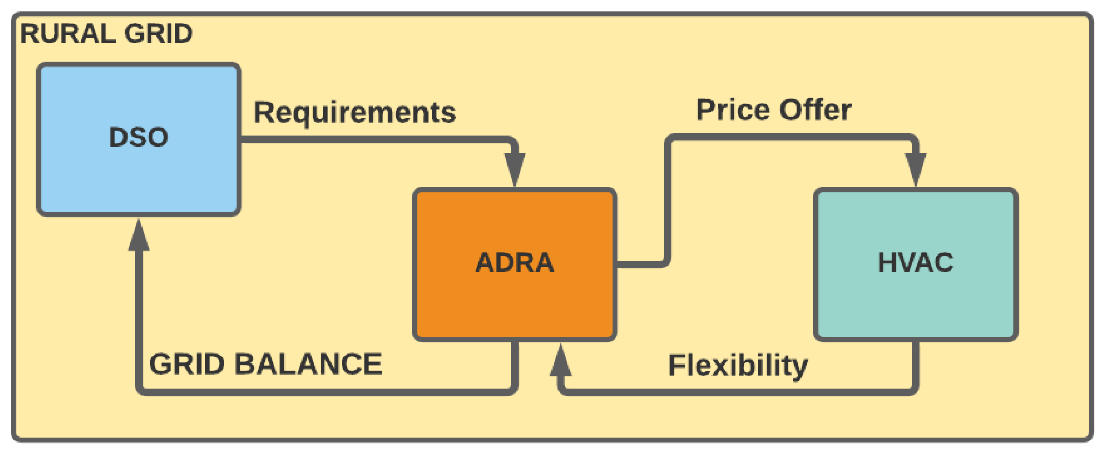
This study aims to improve grid balance (in the interest of the Distributed System Operator (DSO)), control energy, utilize the flexibility of a flower greenhouse (in the customer’s interest), and increase ADRA profit. Figure 1 illustrates the flexible market design.
According to Figure 1, the DSO or retailer is in charge of operating the rural grid and monitoring the threshold levels continuously. When the grid is near or at capacity, the DSO requests that the ADRA increase or decrease end-user use to maintain grid balance. The ADRA analyzes the DSO’s requirements and differential pricing to detect changes in end-user demand. The ADRA transmits price signals that cause end-users to modify the setpoint, preventing imbalances. The HVAC or the client can alter his pattern plan by adjusting the setpoint value. In other words, the DSO instructs the ADRA to alter consumer behavior.
It is necessary to consider the responsibilities of three critical players. The DSO’s primary responsibility is to maintain the grid operational (balance). The ADRA must establish a contract-based pricing structure, and the HVAC system must reduce energy consumption and increase flexibility. The ADRA charges user prices, and the sequence is explained as follows.
- First, the ADRA decides the pricing scheme (ToU, Fixed, or Hourly) that optimizes its objective function depending on the grid requirements. Then, to guarantee grid balance, it creates a time-variant using an hourly time scale.
- Second, the flower greenhouse selects the setpoint value based on the pricing signal, indicating the amount of energy consumed by the HVAC system (on/off sequence) throughout each minute. Consumers are rational agents who want to minimize their costs in this formulation.
The ADRA is a price taker, and the consumer does not know the energy demand for the next day in advance. The HVAC system for the flower greenhouse makes energy consumption (setpoint) decisions based on daily price schemes. The flower greenhouse HVAC system cannot supply energy to the grid or for self-consumption.
Although the flower greenhouse must maintain the flowers for future marketing, it cannot restore grid operation. Additionally, the flower greenhouse HVAC system is considered a client capable of entrusting a portion of their consumption to a load management service in exchange for a fair price. Moreover, it signifies that the buyer is prudent in selecting the most effective alternative available.
Finally, the approach considers the decision-making process on a two-time scale. Upper-level pricing varies hourly depending on the method (ToU, Fixed, or Hourly). The mixed-integer linear problem HVAC model is at the lowest level. The lower-level objective minimizes the number of ON/OFF sequences performed per minute. This suggests that the HVAC decides on a minute-by-minute basis whether to switch on or off the air conditioning to cool the flowers. Unlike a conventional solution, this technique adds HVAC ON/OFF behavior (binary variables) into the Bi-MILP optimization problem. The HVAC model behavior is built based on the proposals described in [42,43].
2.1. Prices
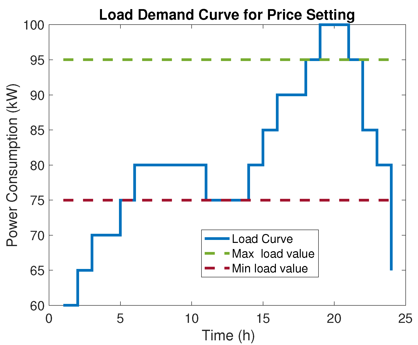
The contract stipulates a maximum and minimum price of and , respectively. These values are established by the Energy, Gas, and Fuel Regulation Commission’s (CREG) standards in accordance with CREG 015-2018 (Resolution No. 015 of 2018 Colombian Energy, Gas, and Fuel Regulation Commission. https://bit.ly/3m5lugD, accessed on (15 April 2022), CREG is the Colombian entity attached to the Ministry of Mines and Energy responsible for regulating electricity and gas services as established in laws 142 and 143 of 1994. The National Government of Colombia created it to regulate public service activities). The pricing computing values are related to the classification of load intervals using a typical load curve , as illustrated in Figure 2, read from commercial borders using measurement equipment.
The conventional method for establishing these load intervals is to calculate the percentage of load carried by the system during a given period concerning the maximum daily load. The computation procedure uses the categorization findings to establish the times of day when the grid is at its peak, average, and minimum load and correlates these numbers to the maximum, mean, and minimum pricing, respectively. Figure 2 illustrates the typical load curve that is employed to calculate these values. This curve is similar to a duck curve, except that i symbolizes the 24 h of the day, and is used to establish the maximum, average, and minimum prices [44,45]. The approach is illustrated in detail in Appendix C.
Figure 2 shows three zones where is above the green line for , between the green and red lines , and below the red line . It is essential to consider that during the hours with a load in the upper (green line), the price is maximum, and between (red line) and (green line), the average price is computed. Furthermore, the minimum price is below (red line). The process to obtain the prices , and solves the following equation system:
where is a factor for the hourly charges of the grid. , , and are vectors (parameters) associated with the hours of the day that have , , and loads, respectively. , , and are the power values associated with the hours of , , and load values, respectively, and is the fixed charge using the grid operator. After solving (1), (2), and (3), the results are the , , and . These values allow the ADRA to design its pricing schemes without violating the limits. As is mentioned above, this research has three different ADRA pricing options that are explained as follows:
- Time of Use: According to our research, this method divides the 24 h of the day into three strips of 8 h. According to the contract criteria, the Bi-MILP model decides the time of occurrence and the , , and of each. To ensure that the pricing plan benefits the grid, the ADRA employs the and values during hours when the flower greenhouse’s consumption must be reduced or increased.
- Fixed: During the 24 h of this program, the ADRA maintains a flat pricing of . The flower greenhouse can choose the setpoint in this scheme based on its requirements.
- Hourly: The Bi-MILP optimization problem solution creates pricing depending on grid requirements in this technique. Only the Stackelberg interaction establishes the values , , or .
2.2. HVAC Behavior Control Modeling
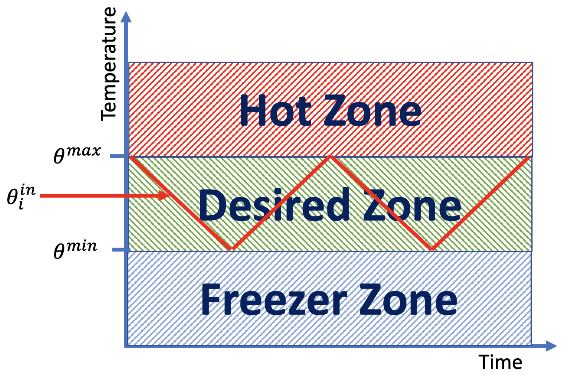
An ON/OFF controller regulates the HVAC system’s primary operation. These controllers incorporate a thermostat to minimize switching when the temperature is near the setpoint. The HVAC’s operating characteristics are illustrated in Figure 3 and correspond to the desired operation of a cold room. All refrigeration systems have three zones: hot, freezer, and desired.
In this research, the aim is to make the indoor temperature of a day stay within desired values . The indoor temperature behavior is depicted in Figure 3; notice that is within the green zone and change between the threshold temperature values and . This change depends on thermostat behavior.
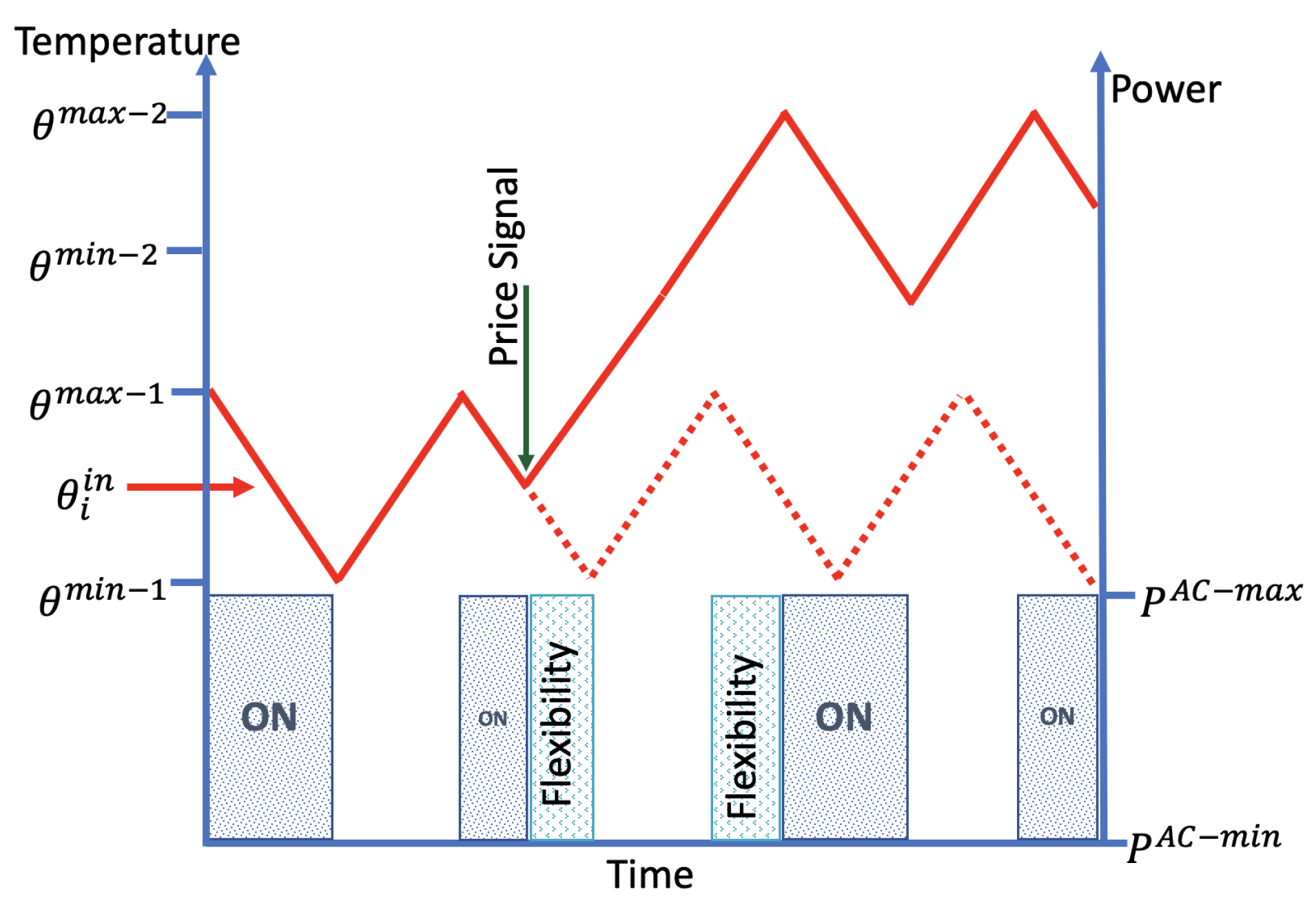
The thermostat is in charge of maintaining within the desired zone. The energy consumption pattern is depicted in Figure 4. The device consumes a maximum power value . During the ON state, reaches the minimum possible operation temperature . Then, the HVAC has to change to the OFF state. In this state, HVAC consumes minimum power values typically, , and allows to reach the maximum temperature value available . This behavior is repeated ensuring .
The lower and upper limits can change depending on the requirements or convenience. This variation of the setpoint makes it possible for HVACs to provide flexible services. The strategy is to reduce power consumption by changing the setpoint operation in response to pricing signals and providing flexible services to support the grid balance. Figure 4 shows the behavior of rational consumers when a signal (higher) price appears. The consumer has a target price to pay, commonly the average price value. If the price of energy exceeds the average value (high price), the setpoint goes from to and, consequently, from to , which means the setpoint changes, e.g., from the range 2–3 C to the range 3–4 C, as is in Figure 4.
Figure 4 shows what flexible service means in this research. The change in the consumption patterns creates the possibility of providing load change as a percentage of flexibility to the grid. This behavior allows establishing a flexible percentage-related setpoint, such as a value for each degree centigrade of indoor temperature change.
3. Flexible DSO-ADRA-HVAC Model and Reformulation
The application presented in this work is modeled as a Bi-MILP optimization problem with upper and lower-level objective functions. The ADRA objective Function (4) is stated to maintain the balance between produced and consumed. The ADRA has to design the consumer price based on contract constraints. is the amount of energy that the ADRA supplies to the consumer. The ADRA acts as a price taker, then depicts the DSO price, and the energy available. The ADRA designs prices on hourly scales, where represents every hour of a day. The consumer decides in a minute scale denoted by j the minutes of one day . The ADRA decides in advance compared with the consumer:
The ADRA must maintain the contract conditions. From above, the constraint (5) makes the ADRA not experience losses by designing a price cheaper than the DSO price . In (6), the ADRA ensures no over cost in the energy service by setting a maximum available price , and (7) is the constraint that guarantees that, at the end of the day or 24 h, the price scheme is equivalent to an average price. This means the end-user is not charged with additional charges rather than the DSO average price. The advantage of signing contracts with the ADRA is to receive payments through the flexibility services. Constraint (8) is the linking constraint of the bi-level problem between the upper and lower level, where represents the consumption of the HVAC system, represents the turning ON/OFF signal, represents the time step , and kW is the HVAC’s nominal power.
In this approach, the ADRA buys energy from DSO, where the price formation is ex-post. Therefore, the ADRA designs prices for the flower greenhouse, and the consumer does not know the energy demand for the next day in advance. Consequently, the flower greenhouse HVAC decides which amount of energy consumption (setpoint) in response to pricing schemes within the daily operation. The current proposal has an optimization problem (ADRA problem (4)) constrained by another optimization problem (HVAC problem (9)). The HVAC flower greenhouse model is stated in constraint (9), which represents the lower-level objective function:
In (9), represents the signal that the HVAC has to minimize. is an ADRA price designed in the upper level. is the nominal power of the HVAC unit equal to kW, and is the time step. The lower optimization problem includes a dynamical behavior of the room as a constraint (10). The indoor temperature is represented by , where are parameters related with the U-values (geometry of the cold room) [42], and represents the load of the cold room due to the flower greenhouse energy consumption by storage.
Constraint (11)–(14) operate to maintain the setpoint within a temperature range (desired zone as in Figure 3). These constraints makes the indoor temperature operate within two different temperature thresholds. As it is shown in Figure 4, the indoor temperature changes from the range – to range – in response to the price signal. It is important to mention that the signal in charge of changing between the two temperature ranges is the binary value . In addition, M and are big values that are used in the model to ensure that the signal makes the indoor temperature stay within the temperature thresholds.
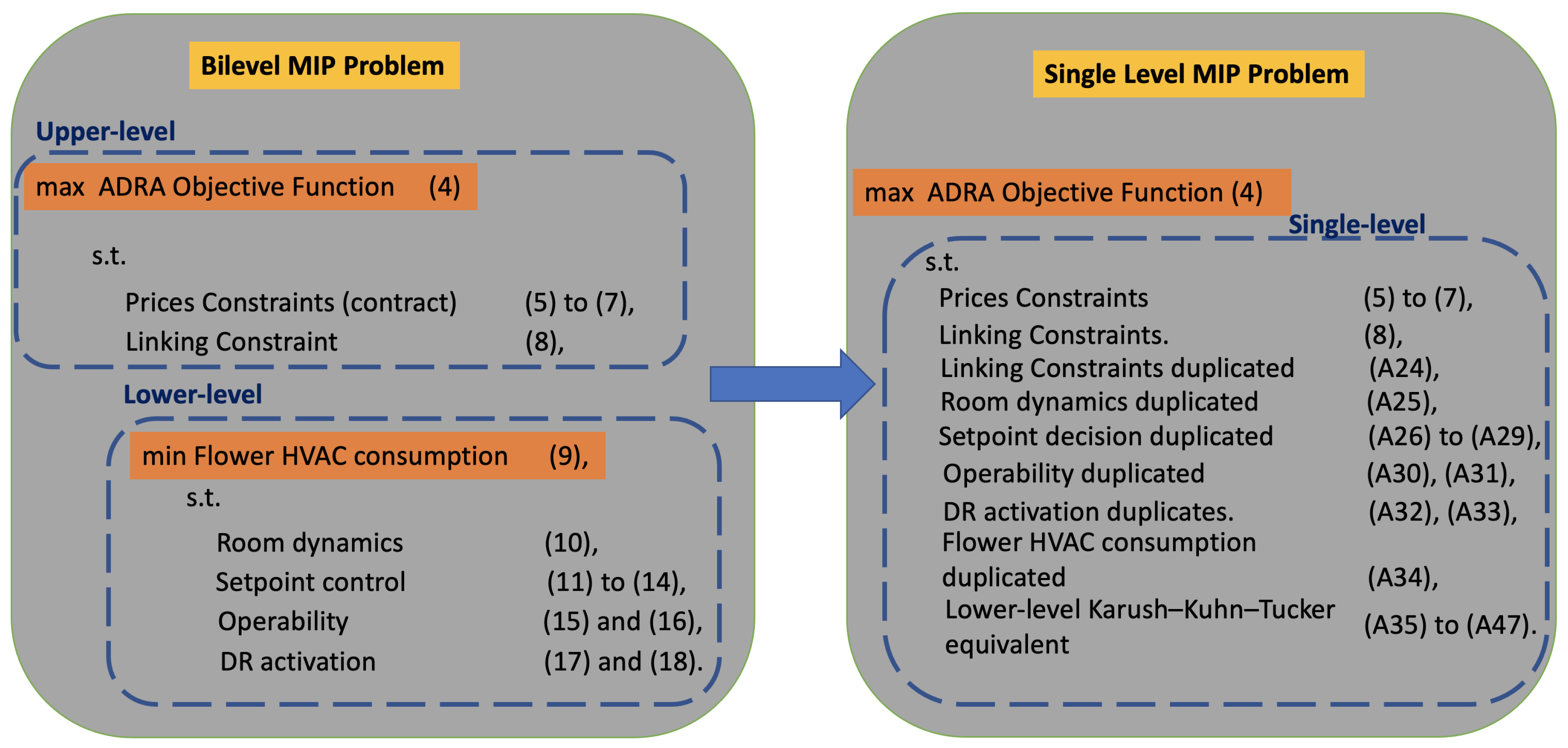
To optimize the ON/OFF sequence , it is necessary to include constraints (15) and (16), where the binary variables and are for avoiding over switching and to ensure consistency of the lower mixed-integer programming model. Finally, it is necessary to ensure the change in load pattern when the price signal appears. For this purpose constraints (17) and (18) are used, where the binary variable is activated when the price exceeds a threshold. The flower greenhouse model is as from (9) to (19). The whole Bi-MILP problem is stated in Equations (4) to (19). For this purpose, the reformulation procedure of [41] is used. All the parameters, variables, functions ans index information are presented in Appendix A. The theoretical formulation is presented in the Appendix B, the Algorithm A1 is presented in Appendix C and the restated current Bi-MILP proposed in this work is developed in Appendix D. The reformulation procedure is performed to obtain the result resumed in Figure 5. The single-level mixed-integer problem can be solved in an easy form with commercial software and does not require a great number of computational resources.
The cornerstone of the reformulation procedure is to duplicate the lower-level problem’s decision variables and constraints. In addition, it is necessary to include additional variables , where for each inequality constraint guarantee the relatively complete response property [41]; expressly, the duplicated variables are in constraints (A24) to (A34).
In this problem, the upper level makes decisions hourly, while the lower level makes decisions each minute. Constraint (A24) shows the linking power constraint with duplicated values (upper zero indices). In addition, these constraints include the lower level variable , which models the ON/OFF state, and the variable represents the consumer price. Constraint (A25) represents the duplicated variable that represents the indoor temperature of the room. Constraints (A26) to (A29) are used to ensure HVAC turns on for indoor temperatures above the maximum temperature. Moreover, the HVAC turns off when the indoor temperature is below a minimum temperature. In these constraints, the variable has the task of informing when the price goes over the average price, and the flower greenhouse changes the setpoint in response to that.
Constraints (A30) and (A31) are for the consistency in the MILP HVAC model and for avoiding over-switching in the HVAC. Finally, constraints (A32) and (A33) are used to activate the DR signal. Constraint (A34) represents the constraint related to the follower objective, and the variables , where represents the number of constraints for ensuring the relatively complete response property of the problem, are also included. The final step of the reformulation procedure is to use the Karush–Kuhn–Tucker (KKT) conditions transformation applied to the lower-level problem (9) to (19), and the KKT equivalent is shown from (A35) to (A47). Finally, the whole single-level optimization problem is shown in Figure 5, where the reformulation results of a single-level MIP problem is stated.
4. Simulations and Results
This section simulates the DSO-ADRA-HVAC approach, which is developed to provide grid flexibility in a local energy market. One of the primary objectives of the research is to establish the degree of flexibility that HVAC can provide to the rural grid to maintain grid balance. The other objective is to assess the three distinct pricing schemes and demonstrate the relative merits and demerits in light of the player interests. Following the reformulation described previously, the Bi-MILP optimization issue is written in GAMS Distribution and solved using the NEOS SERVER tool via the solver ANTIGONE (Algorithms for Continuous-Integer Global Optimization of Nonlinear Equations).
4.1. Flexible Capability
The procedure executed for computing the flexible capability of the HVAC greenhouse is performed by setting conditions and simulating the MILP HVAC model to obtain the results. The Flower HVAC has a constrained indoor temperature operation. The flowers cannot be exposed to temperatures above 6 C for more than 12 h because the maturation process accelerates. The ideal indoor temperature is 2 C and 3 C to adhere to stringent export regulations and ensure exceptional size, color, and durability. This operational condition implies that the HVAC at maximum can change the setpoint value in 3 C going from 2 to 3 C (ideal indoor temperature) to 5 to 6 C (maximum allowed temperature). Taking into account the above consideration, first, a simulation is performed to know the consumption in (kWh) of the cold room when it is set in the range of 2–3 C for 12 h. The HVAC consumes kWh, in the range 2 to 3 C. This consumption is selected as the energy baseload.
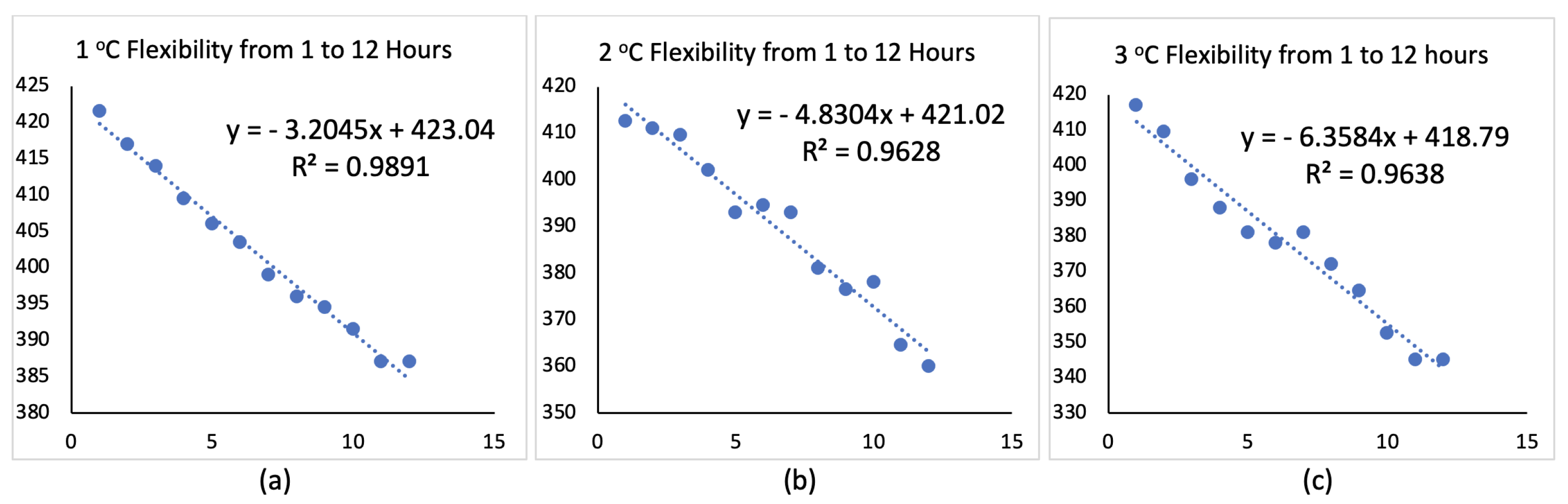
The flexible evaluation results are in Table 1. In this table, four columns represent the number of hours the HVAC provide flexibility services (first column) and the setpoint change in centigrade degrees that the cold room changes (second to fourth columns). Each of the rows of the columns is related to the time that the cold room has to change the flower temperature refrigeration value.
As an objective of relating a quantity of flexible energy for each grade centigrade setpoint change, the data compiled in Table 1 are computed as is shown in Figure 6. For better understanding, the row 5 of Table 1 shows that the end-user has three options for support flexible services for five hours, changing the setpoint to one, two, or a maximum of three degrees centigrades. If the cold room only changes by 1 °C, the consumption is 406 kWh. If it changes by 2 °C , the consumption is 393 kWh, and finally, if it decides to change by 3 C, the consumption is 381 kWh. Depending on the setpoint variation, the end-user can provide , , and up to of his energy consumption in response to grid requirements.
From Figure 6, it is possible to establish the relation between power consumption and the number of hours that change the setpoint to 1 C, 2 C, or 3 C. This analysis is consequential to the grid because when the DSO monitoring system detects a possible emergency status, it requests flexibility from the ADRA, and the ADRA publishes a new price. The flower greenhouse HVAC can decide its setpoint depending on grid requirements in response to this behavior. According to Figure 6, it is possible to establish that the flower greenhouse can support , , or up to flexibility over 12 h.
4.2. Pricing Schemes
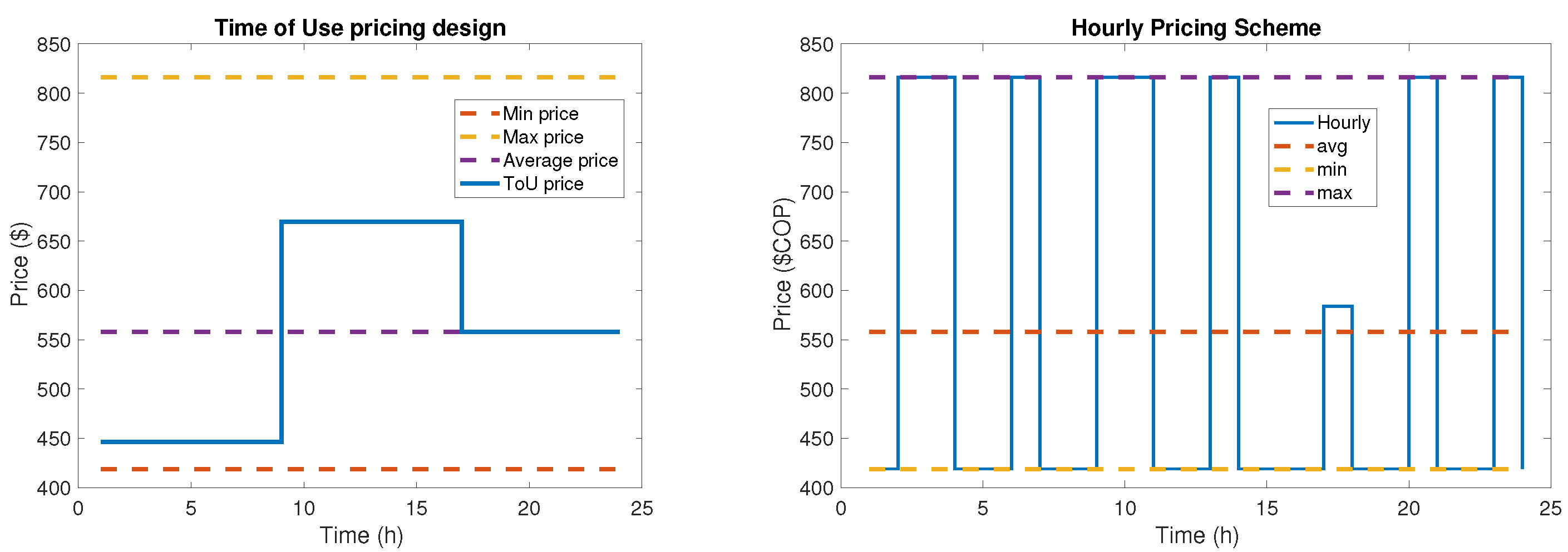
The effect of Time of Use and hourly pricing plans is depicted in Figure 7. In both designs, the tariff for each hour is established by the Stackelberg formulation of the Bi-MIP. It is critical to highlight that the statistics show the pricing threshold limits. The consumer price cannot exceed the maximum price (yellow line), it cannot be less than the minimum price (orange line), and the mean price must be equal to the daily average price (purple line) over 24 h.
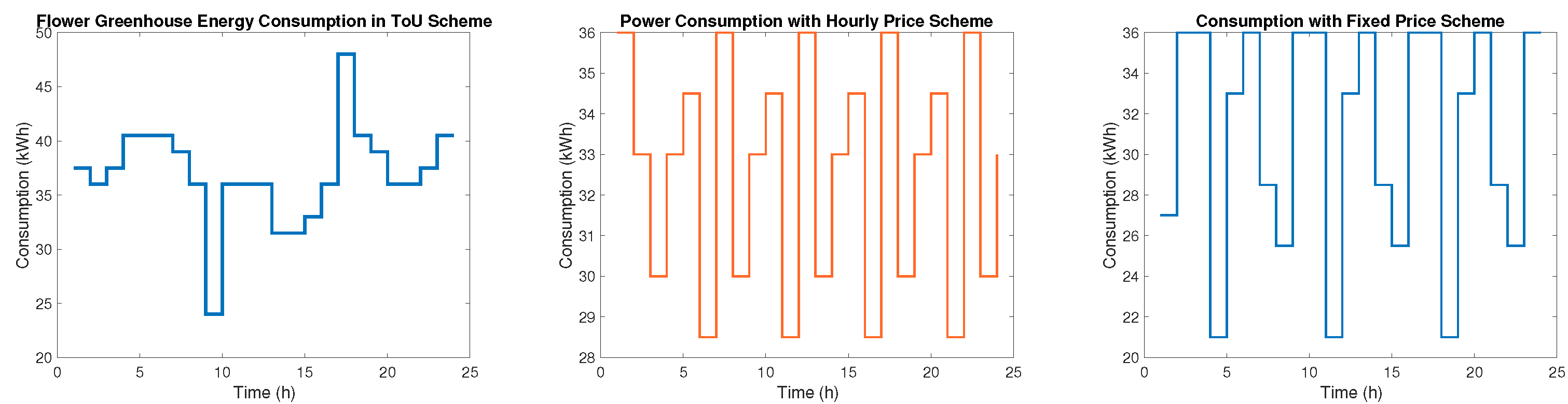
Figure 8 shows the energy consumption pattern of the flower greenhouse HVAC in response to the pricing schemes. From this figure, it is possible to see that energy has an expected behavior in the sense that when the ToU price change from the to , HVAC decreases its energy use to a minimum value in the hour eight of the day. Then, in hour 16 of the day, the ToU changes the price from to a day’s average price . The green flower house over the ToU pricing scheme has an energy level during the 24 h of 747 kWh. The grid does not need the end-user to reduce the pattern when the average price is set. The energy value of the day of this pricing scheme is shown in Table 2. In the hourly pricing plan, the Stackelberg formulation of the Bi-MIP decides the tariff of each one of the hours. Constraints for the pricing design are that the consumer price cannot exceed the max price obtained at the spot price. The consumer price cannot be lower than the minimum price obtained at the spot price, and during the 24 h, the mean price has to be equal to the daily average price.
Finally, since end-users are rational consumers when prices exceed a certain threshold, the setpoint must shift from one range to another with reduced consumption. This operation is performed because the user selects the optimal alternative. The outcomes of the three pricing strategies are shown in Table 2.
The simulations are presented for each price proposal to establish the quantity of energy the end-user consumes each day and month, money savings, and how much flexibility they will provide the grid. The results of the price plan simulations are provided in Table 2. There are seven columns in this table. The pricing structure consists of fixed Time of Use and hourly rates. Additionally, the table illustrates the setpoint shift that the flower greenhouse suffers if it chooses to give flexibility.
The fixed program provides flexibility regarding pricing scheme results if the grid experiences an energy excess and requests an increase in end-user demand. The price is set equal to the daily average price in this pricing scheme, and users are not required to modify the setpoint procedure. In ToU and hourly pricing schemes, both the end-user and the grid can benefit from advanced pricing. The simulation findings indicate that the ToU program can supply the grid with up to 5% of its daily energy usage. This flexibility service provided to the grid saves around 7% on its energy bills. Compared to the ToU program, the hourly plan is the more attractive option because it allows the end-user to save up to 13% on his energy bill and support up to 6% of his energy use to the grid.
5. Conclusions and Future Work
This document proposed a pricing structure for a local energy market that includes an ADRA and a flower greenhouse HVAC system. A Stackelberg game was used to model the local energy market by developing a bilevel mixed-integer linear problem to represent the players’ interests. The problem was reformulated using a decomposition approach to generate a restricted mathematical program with complimentary constraints, which was then solved using the GAMS and Neos Server tools via the solver ANTIGONE (Algorithms for Continuous/Integer Global Optimization of Nonlinear Equations).
The research findings were possible due to the reformulation procedure, which enables the bordering of several classes of mixed-integer problems by creating a duplicated complicated variable set and, depending on the nature of the problem, by including additional continuous functions to ensure a relatively complete response. The CREG normative was employed to calculate the pricing thresholds (, , and ). These values were used to calculate the pricing for the three different plans. The simulations of Time of Use, fixed, and hourly schemes indicate that the flower greenhouse HVAC system can provide up to 20% flexibility. This behavior translates into financial savings for the end customer. If the DSO has a contingency, the end-user might assist by 20% of his usage under specified conditions and for 12 h.
The future study will consider the uncertainty associated with renewable energy adoption. It is necessary to investigate scenarios for photovoltaic generation and stochastic formulations. Furthermore, a new variable will be introduced to reflect flower consumption per kW. This value is calculated using monthly data on energy usage measured in flower stem equivalents per kilowatt.
Author Contributions
Methodology J.S.R., J.V., D.P. and C.A.C.-F.; simulation, J.S.R. and J.V.; validation, J.S.R., J.V., D.P. and C.A.C.-F.; formal analysis, J.S.R., J.V., D.P. and C.A.C.-F.; research, J.S.R., J.V., D.P. and C.A.C.-F.; physical resources, J.S.R.; writing—original draft preparation, J.S.R.; writing—review and editing, J.S.R., J.V., D.P. and C.A.C.-F.; design, J.S.R.; supervision, J.V. and D.P.; project administration, J.S.R., J.V., D.P. and C.A.C.-F.; funding acquisition, J.S.R. and D.P. All authors have read and agreed to the published version of the manuscript.
Funding
This research is funded by Boyacá government grant number 779 of 2017, and Pontificia Universidad Javeriana with project SIAP-00010099.
Institutional Review Board Statement
Not applicable.
Informed Consent Statement
Not applicable.
Data Availability Statement
Not applicable.
Acknowledgments
Boyacá Department of (Colombia) funded this study project, which is developed at the Pontificia Universidad Javeriana-Bogotá. The whole project, of which this study is a part, aims to give farmers in the region with instruments to increase their productivity and economic revenue through crop transformation, thereby improving the quality of farmers’ lives.
Conflicts of Interest
No conflict of interest are declared by the authors.
Abbreviations
The following abbreviations are used in this manuscript:
| DANE | National Planning Departmen |
| ADRA | Agricultural Demand Response Agreggator |
| Bi-MILP | Bilevel Mixed Integer Linear Problem |
| Clombian Peso | |
| ASOCOLFLORES | Colombian Association of Flowers Growers |
| CPP | Critical Peak Price |
| DR | Demand Response |
| DSM | Demand Side Management |
| DSO | Distribution System Operator |
| EMS | Energy Management Systems |
| CREG | Energy, Gas, and Fuel Regulation Commission |
| HVAC | Heating Ventilation and Air Conditioned System |
| LEC’s | Local Energy communities |
| LEM | Local Energy Market |
| MILP | Mixed Integer Linear Programming |
| NIS | National Interconnected System |
| ZNI | Not Interconnected Zone |
| PTR | Peak Time Rebate |
| PIB | Producte Interior Brut |
| RTP | Real-Time Pricing |
| SOs | System Operators |
| ToU | Time of Use |
| TSO | Transmission System Operator |
| Bilevel Optimization Problem | |
| Math Problem Complem. Constraints |
Appendix A. Parameters, Variables, Functions, and Index Information

Table A1.
Parameters, Variables, Functions, and Index Information.
| Definition | PARAMETERS Notation | Units |
|---|---|---|
| Big numbers | , | |
| Building U-values | , , | |
| Factor for hourly charges | ||
| HVAC Nominal Power Consumption | kWh | |
| Maximum Temperature | C | |
| Minimum HVAC Power Consumption | kWh | |
| Minimum Temperature | C | |
| Number of periods in a day | N | |
| Power at hour i | kWh | |
| Time Step | minutes | |
| VARIABLES | ||
| Average Price | ||
| Binary variables | s, a, b, c | |
| Consumer Energy Price | ||
| Demand Response Signal | ||
| DSO Price | ||
| Duplicated Bilevel Optimization Problem | C | |
| Duplicated variables | upper index | |
| Energy consumed by end-user | kWh | |
| Energy available for DSO | kWh | |
| Flower Consumption Load | C | |
| Grid operator charge | COP$ | |
| Indoor temperature | C | |
| KKT multipliers | , | |
| Maximum Hour Load | hour | |
| Maximum HVAC Power Consumption | kWh | |
| Maximum Load Value | kWh | |
| Maximum Price | COP$ | |
| Minimum low Load | hour | |
| Minimum Load Value | kWh | |
| Minimum Price | ||
| FUNCTIONS | ||
| Continuous Decision Variables | x, y | |
| Continuous Function | ||
| Functions | f, g, h, A, b, w, v, P, N, R, K | |
| Identity Matrix | I | |
| Definition | INDEX Notation | Units |
| Time Index | j | minutes |
| Time Index | i | hours |
| Constraint index |
Appendix B. Bi-Level Mixed Integer Linear Problem and Theoretical Reformulation
Since its formulation, this issue has stimulated academics’ interest in exploring and implementing bilevel optimization problems. By definition, bi-level optimization issues are those in which one optimization problem’s constraints constitute another problem. Since 1934, the Stackelberg formulation has been used in the application of market economics [46]. The standard formulation states the problem as two parts, the upper and lower level or the leader and follower [47,48]. The follower’s feasible set is established by the leader’s feasible set. According to their nature, bi-level optimization problems may be categorized into four categories as follows [49]:
- 1
- Upper variables are integers, and lower variables are continuous.
- 2
- Upper and lower variables admit integer and continuous values simultaneously.
- 3
- Upper and lower variables are all integers.
- 4
- Lower variables are integers, and the upper variables are continuous.
In the theory methods for Mixed Integer Problems (MIP), but for the purely linear/nonlinear integers, there are minimal algorithms [50]. The general formulation of the Bi-MIP problem developed in this paper is depicted in Equations (A1) to (A4):
In , x represents the leader’s continuous decision variables, y represents the follower’s continuous decision variables, and z represents the discrete follower decision variables. The upper level in Equations (A1) and (A2) and the lower level in Equations (A3) and (A4) have opposite objectives. Commonly, while one of the levels intends to maximize his interests, the other one intends to minimize them. Due to the nature of the Bi-MILP optimization problems, the computing process is not easy, even for the most straightforward bilevel mixed-integer programming (MIP) problem; it is theoretically NP-hard [41]. This research implements a reformulation procedure to represent the Bi-MILP in a constrained mathematical problem.
The purpose of obtaining an equivalent representation is to find a good approximation to the optimal value using commercial software. A decomposition algorithm based on the column-and-constraint generation method is transforming the Bi-MILP into a constrained mathematical program with complementary constraints. This procedure ensures the problem converges to an -optimal solution value within finite operations [41].
The Bi-MILP common approach is as stated in Equations (A1) to (A4). The cornerstone of the reformulation procedure is to duplicate the lower-level problem’s decision variables and constraints. The duplicating problem process result is stated (A5) to (A9):
In , x represents the continuous decision variables of the leader player, and represent the duplicated continuous and discrete decision variables of the follower player, respectively. The duplicating variables and constraints provide a set that incorporates the original upper x level variables and the lower-level variables. The concept behind this decision-maker is that the upper level will be able to use the couple to obtain a simulation of the decision in the lower level, and with this result, it evaluates the impact of that lower-level response. In mathematical terms, under constraints (A8) and (A9), it is clear that the set is the inducible region or feasible set of the Bi-MILP problem. After obtaining the duplicated problem, it is necessary to expand constraints (A7) and (A8). This procedure implies that for any possible (x, y), the remaining lower level has a finite -optimal value. This assumption is similar to establish that the resource is relatively complete if for every , and every possible realization of random data, the lower level problem is feasible. that is, the property. If there exists a tuple in the lower level that does not meet the relatively complete response property, it means the lower level is infeasible. For solving these, it is necessary to introduce additional variables with big-M penalty coefficients for constraint violations. Specifically the procedure replaces the (A8) and (A9) for (A10) and (A11):
where I represents the identity matrix, and represents the additional continuous functions added to each constraint. Furthermore, it is necessary to take into account the following considerations:
- The bilevel optimization problem includes lower level discrete variables, which implies that when it cannot be reduced to the min value, the reformulation steps are useful to derive the solution.
- The inclusion of variables ensures the problem has the relative complete response. Then, this provides a sufficient condition to ensure the existence of an -optimal solution.
- There exists an optimal solution to the extended formulation that is also feasible and optimal to the original one.
Finally, to obtain an MIP problem, it is possible to compute the Karush–Kuhn–Tucker (KKT) conditions of constraints (A10) and (A11), after the KKT procedure, the new constraints are stated in (A12) to (A16), where represents the KKT multiplier, and ⊥ is employed to represent complementary constraints compactly:
The problem stated in can be easily written in a commercial software and do not require a great quantity of computational resources.
Appendix C. Algorithm to Obtain DSO Prices Based on CREG Normative
This appendix shows the Algorithm A1 applied to the load curve shown in Figure 2 to obtain the three zones, where is above the green line for , between the green and red lines for , and below the red line for . It is essential to consider that during the hours with a load upward of (green line), the price is maximum, and between (red line) and (green line), the average price is computed. Furthermore, the minimum price is below (red line).
| Algorithm A1: Executed for Compute Threshold Pricing Values |
 |
Appendix D. Current Approach Reformulation Result
The cornerstone of the reformulation procedure is to duplicate the lower-level problem’s decision variables and constraints. In addition, it is necessary to include additional variables for each inequality constraint to guarantee the relatively complete response property; expressly, the duplicated variables are in constraints (A24) to (A34):
In this problem, the upper level makes decisions hourly while the lower level makes each minute. Constraint (A24) shows the linking power constraint with duplicated values (upper zero indices). In addition, these constraints include the lower-level variable , which models the ON/OFF state, and the variable represents the consumer price. Constraint (A25) represents the duplicated variable that represents the indoor temperature of the room. Constraints (A26) to (A29) are used to ensure the HVAC turns on for indoor temperatures above the maximum temperature. In addition, HVAC turns off when the indoor temperature goes below a minimum temperature. In these constraints, the variable has the task of informing when the price goes over the average price, and the flower greenhouse changes the setpoint in response to that.
Constraints (A30) and (A31) are for the consistency of the MILP HVAC model and for avoiding over switching in the HVAC. Finally, constraints (A32) and (A33) are used to activate the DR signal. Constraint (A34) represents the constraint related to the follower objective, and the variables , where represents the number of constraints for ensuring the relatively complete response property of the problem, are included:
The final step of the reformulation procedure is to use the Karush–Kuhn–Tucker (KKT) conditions transformation applied to the lower-level problem (9) to (19), and the KKT equivalent is shown from (A35) to (47). Finally, the whole single-level optimization problem is as in Figure 5, where the reformulation result to a single-level MIP problem is stated.
References
- Velásquez, D.; Sánchez, A.; Sarmiento, S.; Toro, M.; Maiza, M.; Sierra, B. A Method for Detecting Coffee Leaf Rust through Wireless Sensor Networks, Remote Sensing, and Deep Learning: Case Study of the Caturra Variety in Colombia. Appl. Sci. 2020, 10, 697. [Google Scholar] [CrossRef] [Green Version]
- Suárez, H.L.A.; Angarita, G.P.G.; Castañeda, L.N.R.; Castro, P.P.C. Illicit Crops, Planning of Substitution with Sustainable Crops Based on Remote Sensing: Application in the Sierra Nevada of Santa Marta, Colombia. In Climate Emergency—Managing, Building, and Delivering the Sustainable Development Goals; Springer: Berlin/Heidelberg, Germany, 2022; pp. 483–494. [Google Scholar]
- Bautista, C.J.; Aldemar Fonseca, Y.; Pardo-Beainy, C. Plum selection system using computer vision. In Proceedings of the 2020 IEEE ANDESCON, Quito, Ecuador, 13–16 October 2020; pp. 1–6. [Google Scholar] [CrossRef]
- Bozchalui, M.C.; Cañizares, C.A.; Bhattacharya, K. Optimal Energy Management of Greenhouses in Smart Grids. IEEE Trans. Smart Grid 2015, 6, 827–835. [Google Scholar] [CrossRef]
- Liu, J.; Chai, Y.; Xiang, Y.; Zhang, X.; Gou, S.; Liu, Y. Clean energy consumption of power systems towards smart agriculture: Roadmap, bottlenecks and technologies. CSEE J. Power Energy Syst. 2018, 4, 273–282. [Google Scholar] [CrossRef]
- Sun, D. Handbook of Frozen Food Processing and Packaging; CRC Press: Boca Raton, FL, USA, 2012. [Google Scholar] [CrossRef]
- Kubo, H.; Murayama, S.; Tanimoto, M.; Okoso, K.; Maeno, S. A possibility of open zero energy plant factory. In Proceedings of the 2016 Electronics Goes Green 2016+(EGG), Berlin, Germany, 6–9 September 2016; pp. 1–8. [Google Scholar]
- Aste, N.; Pero, C.D.; Leonforte, F. Active refrigeration technologies for food preservation in humanitarian context—A review. Sustain. Energy Technol. Assess. 2017, 22, 150–160. [Google Scholar] [CrossRef]
- Golmohamadi, H.; Keypour, R.; Bak-Jensen, B.; Pillai, J.R. Optimization of household energy consumption towards day-ahead retail electricity price in home energy management systems. Sustain. Cities Soc. 2019, 47, 101468. [Google Scholar] [CrossRef]
- Pourghaderi, N.; Fotuhi-Firuzabad, M.; Moeini-Aghtaie, M.; Kabirifar, M. Commercial demand response programs in bidding of a technical virtual power plant. IEEE Trans. Ind. Inform. 2018, 14, 5100–5111. [Google Scholar] [CrossRef]
- Golmohamadi, H.; Keypour, R.; Bak-Jensen, B.; Pillai, J.R.; Khooban, M.H. Robust self-scheduling of operational processes for industrial demand response aggregators. IEEE Trans. Ind. Electron. 2019, 67, 1387–1395. [Google Scholar] [CrossRef] [Green Version]
- Chen, L.; Xu, Q.; Yang, Y.; Song, J. Optimal energy management of smart building for peak shaving considering multi-energy flexibility measures. Energy Build. 2021, 241, 110932. [Google Scholar] [CrossRef]
- Aghajanzadeh, A.; Therkelsen, P. Agricultural demand response for decarbonizing the electricity grid. J. Clean. Prod. 2019, 220, 827–835. [Google Scholar] [CrossRef] [Green Version]
- Endo, A.; Tsurita, I.; Burnett, K.; Orencio, P.M. A review of the current state of research on the water, energy, and food nexus. J. Hydrol. Reg. Stud. 2017, 11, 20–30. [Google Scholar] [CrossRef] [Green Version]
- Bakelli, Y.; Kaabeche, A. Optimal size of photovoltaic pumping system using nature-inspired algorithms. Int. Trans. Electr. Energy Syst. 2019, 29, e12045. [Google Scholar] [CrossRef]
- Chrouta, J.; Chakchouk, W.; Zaafouri, A.; Jemli, M. Modeling and control of an irrigation station process using heterogeneous cuckoo search algorithm and fuzzy logic controller. IEEE Trans. Ind. Appl. 2018, 55, 976–990. [Google Scholar] [CrossRef]
- Santana-Sarmiento, F.; Velázquez-Medina, S. Development of a Territorial Planning Model of Wind and Photovoltaic Energy Plants for Self-Consumption as a Low Carbon Strategy. Complexity 2021, 2021, 6617745. [Google Scholar] [CrossRef]
- Horstink, L.; Wittmayer, J.M.; Ng, K. Pluralising the European energy landscape: Collective renewable energy prosumers and the EU’s clean energy vision. Energy Policy 2021, 153, 112262. [Google Scholar] [CrossRef]
- McPherson, M.; Stoll, B. Demand response for variable renewable energy integration: A proposed approach and its impacts. Energy 2020, 197, 117205. [Google Scholar] [CrossRef]
- Olivella-Rosell, P.; Lloret-Gallego, P.; Munné-Collado, I.; Villafafila-Robles, R.; Sumper, A.; Ottessen, S.Ø; Rajasekharan, J.; Bremdal, B.A. Local Flexibility Market Design for Aggregators Providing Multiple Flexibility Services at Distribution Network Level. Energies 2018, 11, 822. [Google Scholar] [CrossRef] [Green Version]
- Golmohamadi, H. Operational scheduling of responsive prosumer farms for day-ahead peak shaving by agricultural demand response aggregators. Int. J. Energy Res. 2021, 45, 938–960. [Google Scholar] [CrossRef]
- Golmohamadi, H.; Asadi, A. A multi-stage stochastic energy management of responsive irrigation pumps in dynamic electricity markets. Appl. Energy 2020, 265, 114804. [Google Scholar] [CrossRef]
- Golmohamadi, H. Agricultural Demand Response Aggregators in Electricity Markets: Structure, Challenges and Practical Solutions-a Tutorial for Energy Experts. Technol. Econ. Smart Grids Sustain. Energy 2020, 5, 1–17. [Google Scholar] [CrossRef]
- Golmohamadi, H.; Keypour, R. A bi-level robust optimization model to determine retail electricity price in presence of a significant number of invisible solar sites. Sustain. Energy Grids Netw. 2018, 13, 93–111. [Google Scholar] [CrossRef]
- Bessler, S.; Drenjanac, D.; Hasenleithner, E.; Ahmed-Khan, S.; Silva, N. Using flexibility information for energy demand optimization in the low voltage grid. In Proceedings of the 2015 International Conference on Smart Cities and Green ICT Systems (SMARTGREENS), Lisbon, Portugal, 20–22 May 2015; pp. 1–9. [Google Scholar]
- Cui, B.; Joe, J.; Munk, J.; Sun, J.; Kuruganti, T. Load Flexibility Analysis of Residential HVAC and Water Heating and Commercial Refrigeration; Technical Report; Oak Ridge National Lab. (ORNL): Oak Ridge, TN, USA, 2019. [Google Scholar]
- Munankarmi, P.; Jin, X.; Ding, F.; Zhao, C. Quantification of load flexibility in residential buildings using home energy management systems. In Proceedings of the 2020 American Control Conference (ACC), Denver, CO, USA, 1–3 July 2020; pp. 1311–1316. [Google Scholar]
- Du, C.; Li, B.; Yu, W.; Liu, H.; Yao, R. Energy flexibility for heating and cooling based on seasonal occupant thermal adaptation in mixed-mode residential buildings. Energy 2019, 189, 116339. [Google Scholar] [CrossRef]
- Huang, S.; Wu, D. Validation on aggregate flexibility from residential air conditioning systems for building-to-grid integration. Energy Build. 2019, 200, 58–67. [Google Scholar] [CrossRef]
- Wang, B.; Zheng, M.; Lu, Y.; Wu, J.; Zhou, J.; Wu, Z.; Zhao, K. Research on the characteristics of flexible control load of rural distribution network and flexibility evaluation. In Proceedings of the 2021 IEEE 4th Advanced Information Management, Communicates, Electronic and Automation Control Conference (IMCEC), Chongqing, China, 18–20 June 2021; Volume 4, pp. 1125–1130. [Google Scholar] [CrossRef]
- Yoshida, A.; Manomivibool, P.; Tasaki, T.; Unroj, P. Qualitative Study on Electricity Consumption of Urban and Rural Households in Chiang Rai, Thailand, with a Focus on Ownership and Use of Air Conditioners. Sustainability 2020, 12, 5796. [Google Scholar] [CrossRef]
- Tushar, W.; Zhang, J.A.; Smith, D.B.; Poor, H.V.; Thiébaux, S. Prioritizing Consumers in Smart Grid: A Game Theoretic Approach. IEEE Trans. Smart Grid 2014, 5, 1429–1438. [Google Scholar] [CrossRef] [Green Version]
- Mohan, V.; Suresh, M.P.R.; Singh, J.G.; Ongsakul, W.; Kumar, B.K. Online optimal power management considering electric vehicles, load curtailment and grid trade in a microgrid energy market. In Proceedings of the 2015 IEEE Innovative Smart Grid Technologies—Asia (ISGT ASIA), Bangkok, Thailand, 3–6 November 2015; pp. 1–6. [Google Scholar] [CrossRef]
- Garcia-Torres, F.; Bordons, C.; Tobajas, J.; Real-Calvo, R.; Chiquero, I.S.; Grieu, S. Stochastic Optimization of Microgrids with Hybrid Energy Storage Systems for Grid Flexibility Services Considering Energy Forecast Uncertainties. IEEE Trans. Power Syst. 2021, 36, 5537–5547. [Google Scholar] [CrossRef]
- Olivella-Rosell, P.; Rullan, F.; Lloret-Gallego, P.; Prieto-Araujo, E.; Ferrer-San-José, R.; Barja-Martinez, S.; Bjarghov, S.; Lakshmanan, V.; Hentunen, A.; Forsström, J.; et al. Centralised and distributed optimization for aggregated flexibility services provision. IEEE Trans. Smart Grid 2020, 11, 3257–3269. [Google Scholar] [CrossRef] [Green Version]
- Vuelvas, J.; Ruiz, F. Rational consumer decisions in a peak time rebate program. Electr. Power Syst. Res. 2017, 143, 533–543. [Google Scholar] [CrossRef] [Green Version]
- Oprea, S.V.; Bâra, A. Edge and fog computing using IoT for direct load optimization and control with flexibility services for citizen energy communities. Knowl.-Based Syst. 2021, 228, 107293. [Google Scholar] [CrossRef]
- Evangelopoulos, V.A.; Avramidis, I.I.; Georgilakis, P.S. Flexibility services management under uncertainties for power distribution systems: Stochastic scheduling and predictive real-time dispatch. IEEE Access 2020, 8, 38855–38871. [Google Scholar] [CrossRef]
- Laur, A.; Nieto-Martin, J.; Bunn, D.W.; Vicente-Pastor, A. Optimal procurement of flexibility services within electricity distribution networks. Eur. J. Oper. Res. 2020, 285, 34–47. [Google Scholar] [CrossRef]
- Gregoratti, D.; Matamoros, J. Distributed Energy Trading: The Multiple-Microgrid Case. IEEE Trans. Ind. Electron. 2015, 62, 2551–2559. [Google Scholar] [CrossRef] [Green Version]
- Zeng, B.; An, Y. Solving bilevel mixed integer program by reformulations and decomposition. Optim. Online 2014, 1–34. [Google Scholar]
- Antunes, C.H.; Rasouli, V.; Alves, M.J.; Gomes, Á.; Costa, J.J.; Gaspar, A. A discussion of mixed integer linear programming models of thermostatic loads in demand response. In Advances in Energy System Optimization; Birkhä user: Basel, Switzerland, 2020; p. 105. [Google Scholar]
- Soares, I.; Alves, M.J.; Antunes, C.H. Designing time-of-use tariffs in electricity retail markets using a bi-level model–Estimating bounds when the lower level problem cannot be exactly solved. Omega 2020, 93, 102027. [Google Scholar] [CrossRef]
- Garces, A.; Correa, C.A.; Bolaños, R. Optimal operation of distributed energy storage units for minimizing energy losses. In Proceedings of the 2014 IEEE PES Transmission & Distribution Conference and Exposition-Latin America (PES T&D-LA), Medellin, Colombia, 10–13 September 2014; pp. 1–6. [Google Scholar]
- Montaña, S.D.; Correa, C.A. Programación Óptima de Cargas Eléctricas Flexibles a Nivel Residencial en Tiempos de COVID-19. INGE CUC 2021, 1, 17. [Google Scholar] [CrossRef]
- Von Stackelberg, H.; Von, S.H. The Theory of the Market Economy; Oxford University Press: Oxford, UK, 1952. [Google Scholar]
- Bracken, J.; McGill, J.T. Mathematical programs with optimization problems in the constraints. Oper. Res. 1973, 21, 37–44. [Google Scholar] [CrossRef]
- Dempe, S.; Kalashnikov, V.; Pérez-Valdés, G.A.; Kalashnykova, N. Bilevel Programming Problems; Energy Systems Series; Springer: Berlin, Germany, 2015. [Google Scholar]
- Dempe, S.; Kue, F.M. Solving discrete linear bilevel optimization problems using the optimal value reformulation. J. Glob. Optim. 2017, 68, 255–277. [Google Scholar] [CrossRef]
- Gümüş, Z.H.; Floudas, C.A. Global optimization of mixed-integer bilevel programming problems. Comput. Manag. Sci. 2005, 2, 181–212. [Google Scholar] [CrossRef]
Figure 1.
DSO-ADRA-HVAC Flexibility Scheme.

Figure 2.
Typical Load Curve for Price Setting.

Figure 3.
Indoor temperature behavior.

Figure 4.
Load Management—Flexibility Capability.

Figure 5.
Bilevel MIP Problem reformulation into a Single MIP Problem.

Figure 6.
Linear approximation for the flexibility services from 1 to 12 h. In (a) is computed for 1 C change, in (b) for 2 C change, and in (c) for 3 C change.
Figure 6.
Linear approximation for the flexibility services from 1 to 12 h. In (a) is computed for 1 C change, in (b) for 2 C change, and in (c) for 3 C change.

Figure 7.
Pricing Scheme Results.

Figure 8.
Flower Greenhouse Energy Consumption in Response to Pricing Schemes.

Table 1.
HVAC Flower Greenhouse Flexible Consumption Evaluation.
| Hour | (kWh) 3 C to 4 C | (kWh) 4 C to 5 C | (kWh) 5 C to 6 C |
|---|---|---|---|
| 1 | 417 | ||
| 2 | 417 | 411 | |
| 3 | 414 | 396 | |
| 4 | 402 | 388 | |
| 5 | 406 | 393 | 381 |
| 6 | 378 | ||
| 7 | 399 | 393 | 381 |
| 8 | 396 | 381 | 372 |
| 9 | |||
| 10 | 378 | ||
| 11 | 387 | 345 | |
| 12 | 387 | 360 | 345 |
Table 2.
Pricing Schemes Comparison.
| Scheme | Temp. Change (C) | Daily Bill COP | Consumption (kW) | Monthly Bill COP | User Savings | Flexibility |
|---|---|---|---|---|---|---|
| Fixed | 0 | 726,711 | 1302 | 21,801,330 | 0 | 0 |
| ToU | 1 | 709,799 | 1278 | 21,293,970 | 2 | 2 |
| 2 | 691,574 | 1251 | 20,746,410 | 5 | 4 | |
| 3 | 677,481 | 1231 | 20,324,430 | 7 | 5 | |
| Hourly | 1 | 682,061 | 1270 | 20,461,830 | 6 | 2 |
| 2 | 657,842 | 1243 | 19,461,830 | 9 | 5 | |
| 3 | 629,550 | 1221 | 18,886,500 | 13 | 6 |
Publisher’s Note: MDPI stays neutral with regard to jurisdictional claims in published maps and institutional affiliations. |
© 2022 by the authors. Licensee MDPI, Basel, Switzerland. This article is an open access article distributed under the terms and conditions of the Creative Commons Attribution (CC BY) license (https://creativecommons.org/licenses/by/4.0/).
Share and Cite
MDPI and ACS Style
Roncancio, J.S.; Vuelvas, J.; Patino, D.; Correa-Flórez, C.A. Flower Greenhouse Energy Management to Offer Local Flexibility Markets. Energies 2022, 15, 4572. https://0-doi-org.brum.beds.ac.uk/10.3390/en15134572
AMA Style
Roncancio JS, Vuelvas J, Patino D, Correa-Flórez CA. Flower Greenhouse Energy Management to Offer Local Flexibility Markets. Energies. 2022; 15(13):4572. https://0-doi-org.brum.beds.ac.uk/10.3390/en15134572
Chicago/Turabian StyleRoncancio, Juan Sebastian, José Vuelvas, Diego Patino, and Carlos Adrián Correa-Flórez. 2022. "Flower Greenhouse Energy Management to Offer Local Flexibility Markets" Energies 15, no. 13: 4572. https://0-doi-org.brum.beds.ac.uk/10.3390/en15134572
Note that from the first issue of 2016, this journal uses article numbers instead of page numbers. See further details here.