Compressed Air Energy Storage Capacity Configuration and Economic Evaluation Considering the Uncertainty of Wind Energy

Abstract

The random nature of wind energy is an important reason for the low energy utilization rate of wind farms. The use of a compressed air energy storage system (CAES) can help reduce the random characteristics of wind power generation while also increasing the utilization rate of wind energy. However, the unreasonable capacity allocation of the CAES system results in high capital investment and a long payback period. In order to improve the economic benefits of energy storage, this paper studies the capacity configuration of compressed air energy storage systems under the condition of wind energy uncertainty. First, the typical hourly power distribution of wind power generation was obtained using historical data. Factors such as user load demand, time-of-use price of the power grid, system investment cost, power shortage cost, and power sales revenue were considered. Then, a model was built with the charging and discharging power and gas storage capacity of the CAES system as constraints, and the maximum return on investment and the minimum volume of the gas storage tank as targets. NSGA-II and TOPSIS optimal selection methods were used to solve the problem. Finally, the model was used to optimize a power operation case. The results show that in the case of an hourly load power demand of a factory using 3.2 MW, a wind farm would need to keep four wind turbines running every day, and a compressed air energy storage system with a rated power of 1 MW and a rated capacity of 7 MW would ensure the best project benefit. In this mode, 1.24 × 10³ MWh of wind abandoning power could be reduced annually, 2.6 × 10⁴ kg of carbon emissions could be reduced by increasing energy storage within the operation cycle, and the payback period of investment would only be 4.8 years.

1. Introduction

Owing to pollution from fossil fuels, renewable energy resources that are clean, environment friendly and inexhaustible will play a major role in modern energy systems. As a renewable energy resource, wind power technology has been widely used in northwest China, especially Inner Mongolia. According to the 14th Five-Year Plan, to match the national strategy of carbon neutrality, wind power generation should strive to reach a target of at least 800 million kW capacity by 2030 [1]. However, high variability and non-determinism associated with wind power have become bottleneck problems which pose major challenges in designing isolated power systems [2]. Energy storage systems (ESS) have become a method to maintain the balance between energy generation and demand. ESS can store surplus energy in off-peak hours and release it during energy-deficient hours; this can overcome the diurnal and seasonal fluctuations of wind power [3]. Many methods, including pumped hydro storage [4], compressed air energy storage (CAES) [5], battery energy storage [6], hydrogen storage systems [7], and flywheel energy storage [8] have been posed. Nevertheless, each energy storage technology has its drawbacks. Pumped hydro storage requires suitable topography, flywheel energy storage has a high capital cost and high daily self-discharge rate of 50–100% [4], and battery energy storage has a short lifetime [9]. CAES technology has been commercially developed since the late 1970s [10]. Among many energy storage technologies, CAES is a relatively viable option due to its advantages of long storage duration, moderate response time, and good part-load performance [11]. CAES can be used in large-scale facilities as well as distributed and small-scale operations [12,13]. There is a growing research interest in CAES technology. Hao Sun et al. proposed a hybrid wind system by integrating a wind turbine with CAES and designed a prototype test rig for proof of the concept. It proved that the proposed hybrid system is feasible technically [14]. Gayathri V. et al. designed a small capacity CAES system by constructing a 400 L capacity storage tank. The round-trip efficiency was obtained at different mass flow rates by experiment [15]. Adewale O. et al. proposed a near-isothermal-isobaric CAES to improve roundtrip efficiency. R134a as the energy storage working fluid was utilized in the system [16]. However, the high cost of CAES is a major obstacle to its application. To reduce the total cost of the CAES system for a given exergy storage capacity, B.C. árdenas et al. [17] investigated an A-CAES system with an innovative operating scheme. Energy was stored in the form of advanced compression heat to enhance the storage efficiency of the system pressure reservoir.

As relevant departments in China pay more and more attention to the standard formulation of energy storage, relevant policies have been initiated, such as the requirement that the energy storage ratio of the power generation terminal should not be lower than 15% of the power generation scale. However, due to the mutual constraints of the overall energy system economy and energy savings, the construction of energy storage systems such as the CAES system has made slow progress. Therefore, scholars from all walks of life have done a lot of exploration in this field. For example, Chen et al. [18], in order to enhance the stability of China’s power grid and alleviate wind intermittency, we developed a new combined energy storage system based on A-CAES and FESS. For a 49.5 MW wind farm, wind power fluctuation could be effectively balanced, and the power abandonment rate of wind power could be kept at 6.6%. In [19], an innovative combination of CAES, solar heliostat and multi-effect thermal vapor compression seawater desalination unit was established to achieve energy savings and efficiency enhancement; with typical verified cases, a payback period of 2.65 years was obtained. The authors of [20] employed artificial neural networks to train model results and employed four multi-objective optimization procedures based on MOPSO, NSGA-II, PEIESA-II, and SPEA2 algorithms to determine the optimum between system thermodynamic performance and economic viability. Asmae B. et al. [10] proposed a new method for energy storage system operation and optimization. The economics of energy storage in solar and wind power facilities were examined in this research. However, the uncertainty of wind power generation and load demand was not considered. The authors of [21] analyzed the power shortage situation of the two wind farms at different time scales and then evaluated the peak distribution and storage potential of the site. It was found that 60 MW or more energy storage could be increased by configuring a compressed air energy storage system with an appropriate scale.

Based on the above literature, researchers have explored the configuration of CAES systems in different application scenarios from multiple perspectives, but due to their own constraints, the energy storage ratio in each scenario is not universal. Energy storage capacity and power output often don’t match, and often cause economic losses. Therefore, in different application scenarios, how to solve the uncertainty of wind power output and load demand, improve wind power generation with respect to its use, and identify the best CAES storage system matching the scale of the power system become key issues in the success of power projects. Taking Shanxi Province as an example, this paper proposes a new method, and new thinking, to balance the uncertain characteristics of wind power generation and optimize the scale of a CAES system for factories with wind power generation as the main power source. Our aim was to establish energy systems including A-CAES, wind farms, power grid companies and factory users to realize energy interconnection. The wind speed interval method (Bin method), Weibull distribution and weighted average method were used to analyze the probability distribution of wind speed and load demand, and a typical hourly power curve was obtained. Then, the power curve was taken as the input parameter of power dispatching, and an economic evaluation model was constructed from the perspective of power generation enterprises. The objective was to maximize the system investment return and minimize the gas storage size. An improved genetic algorithm was used as the computing engine. Finally, the actual operation data of users in a wind farm and factory in Xiaxian were selected as parameter conditions to evaluate the actual effect of the model, optimize the capacity configuration of the energy storage system in corresponding scenarios, and select the optimal power scheduling scheme.

The main contributions of this study are as follows:

• A coordinated energy dispatching system of a wind farm, a A-CAES system and a power grid company was constructed to reduce the waste and mitigate shortage of power caused by natural factors when supplying power to a factory.
• Based on historical yearly wind and user load demand data, the probability distribution of the power index was analyzed, and the hourly power curve under typical working conditions was established to reduce interference at special time points and make data processing more effective.
• Regarding economic and environmental benefits, an evaluation model with investment return and gas storage tank volume as the targets was established. The optimal capacity configuration of the power supply side energy storage system was calculated by NSGA-II combined with the TOPSIS method to ensure objectivity of the optimization results.

A Web APP for capacity configuration of a compressed air energy storage system was built on the MATLAB platform to visualize the entire simulation running process and provide a computing platform for capacity configuration of the energy storage system and power operation planning under typical working conditions. The structure of this paper is as follows. In the second part, the extraction of wind power and load power curves under typical working conditions are determined. Then, the working principle of the compressed air energy storage system is examined and modeling of a three-stage adiabatic compressed air energy storage system is carried out. The third part describes the optimization model framework, including the control CAES system objective function, constraints, and optimization algorithm. The fourth part focuses on case studies, mainly analyzing the advantages and disadvantages of different energy utilization schemes adopted by typical factory users. Finally, the fifth part provides the conclusion and future research directions.

2. Modeling of Wind Power Coupled CAES System

This section introduces a source, storage, and load energy system design scheme, as shown in Figure 1. The system consists of wind farms, grids, compressed air energy storage systems (CAES) and user load demand centers. CAES power plants can overcome the randomness of wind power and alleviate the contradiction between supply and demand. At the same time, in the case of insufficient power, they can also be supplemented by connecting to the local power grid. The structural features of the CAES system are introduced in Section 2.2.

2.1. Uncertainty Models of Simulated Wind Farm and User Demand

The variability and unpredictability of wind power are the two major challenges facing wind energy resource applications [22]. To deal with the first challenge, a combination of equipment, such as CAES with balanced output power and optimization strategies, is very effective. Because of the second challenge, it is often necessary to adjust the power dispatching strategy according to the actual load demand of users.

2.1.1. Hourly Wind and Weibull Distribution

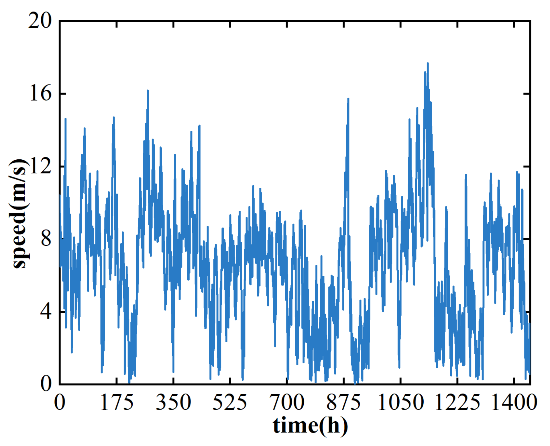
In order to establish an appropriate data processing model, the wind power data of Xia Country Wind Farm in 2019 was collected. Figure 2 shows some of these data. It can be seen from the figure that the wind speed in this region fluctuates considerably. Due to the variability of natural wind power, the power generation of wind farms often varies greatly. Therefore, how to overcome the uncertainty of wind output has become a key problem in model building.

Natural wind fluctuations occur due to seasonal climatic and environmental factors. Instead of using five weighting factors representing days [23] and using Gaussian copulas [24] to fit wind power data to build stochastic models, we used the Weibull probability distribution function [22]. The combination of the Weibull function and the bin interval can effectively overcome the interference of natural factors. It is possible to predict future uncertain wind power by determining the maximum probabilistic power per hour of wind power. The mathematical expression of the Weibull function is as follows:

$$f\left(v\right)=\frac{k}{\lambda }{\left(\frac{v}{\lambda }\right)}^{k-1}{e}^{-{\left(\frac{v}{\lambda }\right)}^k}$$

(1)

where f(v) is the probability density function, k is the shape parameter, and λ is the scale parameter. The specific data processing method is as follows: Take the first hour as an example. First, the data outside the cut-in and cut-out wind speed in the historical wind power data are excluded, and the vacancy values are filled by Newton interpolation method. Second, according to the standard IEC61400-12-1 [25], the effective wind power data between 0 and 1 h are summarized. Then, the wind speed interval [26] method (bin method) is used to divide the interval with the integer multiple of 0.5 m/s [25] as the center, and calculate the wind speed probability density within the interval. Lastly, the parameters of each interval are summarized and analyzed statistically, and the Weibull distribution curve is established. Figure 3 shows the probability diagram of wind speed distribution from 00:00–1:00. When λ = 9.5066 and k = 3.7573, the Weibull function fits the changes of wind speed well and verifies the reliability of Weibull distribution modeling.

The equipment used in the wind farm is a FD70b wind turbine, the parameters of which are shown in

Table 1. FD70b parameter table.

Parameters	Rated Power (MW)	Cut-in Wind Speed (m/s)	Rated Speed (m/s)	Cut-Out Wind Speed (m/s)	Blade Length (m)
Value	1.5	3.5	13	20	34

. In a wind farm, the relationship between the output power of the wind power generation unit and the wind speed is expressed by Equation (2):

$$P_W(t)=\left\{\begin{array}{l}0,v_h(t)<v_{in},v_h(t)>v_{out}\hfill \\ \frac{v_h{(t)}^3-v_{in}^3}{{(v_W^r)}_{}^3-v_{in}^3}{P}_{\mathrm{W}}^r,v_{in}\le v_h(t)<v_{\mathrm{W}}^r\hfill \\ P_W^r,v_{\mathrm{W}}^r\le v_h(t)<v_{out}\hfill \end{array}\right.$$

(2)

where $P_W^r$ is the rated power of the fan, v_h is real-time wind speed, and v_in and v_out are the cut-in and cut-out wind speed, respectively. The relationship between the parameters is shown in Figure 4. As can be seen in the figure, the wind power generation data simulated by Weibull is basically the same as the theoretical output power curve trend of the wind power plant, and can be used as an effective input parameter for economic analysis.

In summary, the main steps of constructing a representative hourly wind power output curve based on the Weibull probability distribution are as follows:

(1)

According to Weibull distribution probability density function, solve the maximum probability wind speed distribution in each interval;

(2)

Calculate the maximum probability output power of the fan in the corresponding interval according to the output characteristics of the fan;

(3)

Use the weighted average method to obtain the expected power per hour. The equation as follows:

$$P_W\left(t\right)=P_{W1}f\left(t,P_{W1}\right)+P_{W2}f\left(t,P_{W2}\right)+\dots +P_{Wi}f\left(t,P_{Wi}\right)+\dots +P_{Wn}f\left(t,P_{Wn}\right)$$

(3)

where P_W(t) is the output power of the fan at t, and f(t, P_Wi) is the probability that the power value is equal to P_Wi at t.

According to the above steps, a typical hourly power curve can be obtained, as shown in Figure 5. The average output power per hour is 0.79 MW.

2.1.2. Hourly User Load Demand

The power demand of the client [27] is uncertain. Therefore, to develop an appropriate power dispatching strategy to meet the users’ demands, the project collected the load demand data of factory users throughout 2019 and analyzed their demand changes. The vacancy values affected by objective factors were filled by an interpolation method. The maximum and minimum load requirements were 3.83 MW and 2.11 MW, respectively. Figure 6 shows the variation of the plant’s load demand from 1–5 August. In view of the rapid variation of user load demand in this factory, we summarized the data of the whole year and calculated the probability distribution of load by an inductive analysis method [28], and then established a typical hourly load demand curve to balance randomness. Figure 7 depicts the probability distribution of load requirements from 00:00 to 1:00.

To construct an hourly load demand power curve based on probability distribution, the procedure was as follows:

(1)

Compute the marginal distribution of hourly load demand by inductive analysis;

(2)

Aggregate load probability distribution data to obtain hourly probability load demand;

(3)

According to step (2), the weighted average method [29] is used to compute, and then the load demand curve is drawn. The mathematical expression is as follows. Where P_L(t) is load demand in time t, P_Li represents load demand value, and f(t, P_Li) is probability when load demand is equal to P_L(t) at time t.

$$P_L\left(t\right)=P_L{}_{1}f\left(t,P_L{}_1\right)+P_L{}_{2}f\left(t,P_L{}_2\right)+\dots +P_L{}_{i}f\left(t,P_L{}_i\right)+\dots +P_{Ln}f\left(t,P_L{}_n\right)$$

(4)

Based on the above steps, a typical hourly load demand curve is shown in Figure 8. It can be seen that the hourly average load demand is 3.241 MW, the load curve trend is smooth, and the peak-to-valley difference is as small as 0.079 MW, which is 2.4% of the peak power. The reason for the above is that the maximum probability load demand per hour in the year obtained after data processing was used to replace the future value to overcome the interference of special days, so the load demand of factory users was relatively stable. At the same time, the extraction of a typical load curve provided theoretical support for the estimation of daily power dispatch.

Due to the uncertainty of actual wind power output and load demand, energy storage planning of power generation enterprises often cannot effectively meet the load demand. Therefore, the uncertainty problem was transformed into a 24-h combined power distribution model based on wind power generation and user load demand, which is more reliable than using a special day to express the uncertainty model and provides a theoretical basis for the early energy storage scale planning of power generation enterprises. The specific parameters are shown in

Table 2. Hourly load demand and wind distribution.

Time (h)	PW (MW)	Weibull		PL (MW)	Time (h)	PW (MW)	Weibull		PL (MW)
		λ	k				λ	k
1	0.98	9.507	3.757	3.214	13	0.52	6.925	3.002	3.224
2	0.96	9.574	4.297	3.223	14	0.50	6.896	2.792	3.230
3	0.92	9.352	4.017	3.236	15	0.55	7.384	2.983	3.252
4	0.87	8.757	4.382	3.259	16	0.57	7.522	2.803	3.235
5	0.78	8.262	3.839	3.237	17	0.64	7.518	2.823	3.223
6	0.83	8.710	3.674	3.263	18	0.71	7.941	3.070	3.250
7	0.84	9.173	3.351	3.240	19	0.82	8.526	3.429	3.259
8	0.88	9.113	3.445	3.257	20	0.90	8.864	3.278	3.247
9	0.85	8.890	3.225	3.215	21	0.98	9.507	3.532	3.279
10	0.73	8.464	3.282	3.204	22	1.04	10.015	3.938	3.244
11	0.57	7.521	2.814	3.228	23	1.05	10.326	4.120	3.283
12	0.52	6.972	3.019	3.251	24	0.99	9.830	3.950	3.235

, forming the theoretical basis for implementing the optimal scheduling policy in Section 3.

2.2. Model of Compressed Air Energy Storage System

The CAES system consists of a compressor unit, motor-generator set, expansion unit and gas storage tank. A diagram is shown in Figure 9. Its essence is a typical three-stage adiabatic compressed air energy storage system coupled to a wind farm. In charging mode, the compressor works with low valley electric energy and surplus electric energy of the wind farm as power source and converts excess wind power into compressed air to accomplish energy storage. In the discharge mode, the high-pressure air stored in the air tank is discharged through a throttle valve to stabilize the output pressure and is coupled with the compression heat to act on the expander to drive the generator.

We established a CAES system model based on the assumptions that air leakage is not considered in each link of gas circulation, and phase change and chemical reaction of fluid in the process of flow and heat exchange are ignored.

2.2.1. Compression Stage Model

The mathematical expression of compression power (charging power) [30] according to the thermodynamic model is:

$$P_{\mathrm{CAES},\mathrm{ch}}(t)={\displaystyle \sum _{i=1}^{N_{\mathrm{com}}}\frac{\gamma R_{\mathrm{g}}}{\gamma -1}}{q}_{\mathrm{com}}(t)\left(T_{\mathrm{com},\mathrm{out},i}-T_{\mathrm{com},\mathrm{in},i}\right)$$

(5)

where η_ch and P_CAES,ch(t) is the charging power and efficiency of the CAES system at t, N_com is the number of compressor stages, γ and R_g are the polytropic index and the gas constant, respectively, q_com is mass flow, T_com,out,i and T_com,in,i are the inlet and outlet temperature, respectively, and π_com,i is the rated compression ratio of class i.

The outlet temperature of the i stage compressor is:

$$T_{\mathrm{com} , \mathrm{out} ,i}=T_{\mathrm{com},\mathrm{in} ,i}\left[1+\left({\pi }_{\mathrm{com} ,i}^{\frac{\gamma -1}{\gamma }}-1\right)/{\eta }_{\mathrm{ch} }\right]$$

(6)

2.2.2. Expansion Stage Model

The mathematical expression of expansion power (discharge power) [30] is:

$$P_{\mathrm{CAES},\mathrm{dis}}(t)={\displaystyle \sum _{i=1}^{N_{\exp }}\frac{\gamma R_{\mathrm{g}}}{\gamma -1}}{q}_{\exp }(t)\left(T_{\exp ,\mathrm{in},i}-T_{\exp , \mathrm{out},i}\right)$$

(7)

where η_dis and P_CAES,dis(t) are the discharge efficiency and discharge power of the CAES system, respectively, N_exp is the number of expander stages, q_exp(t) is mass flow, T_exp,out,i and T_exp,in,i are the inlet and outlet temperature, and π_exp,i is the rated compression ratio of class i.

The outlet temperature of the i stage expander is:

$$T_{\exp ,\mathrm{out},i}=T_{\exp ,\mathrm{in},i}\left[1-\left(1-{\pi }_{\exp ,i}^{\frac{\gamma -1}{\gamma }}\right){\eta }_{\mathrm{dis} }\right]$$

(8)

2.2.3. High-Pressure Gas Storage Stage Model

The gas storage tank adopts an isothermal model. At present, research on the gas storage tank model in the CAES system is generally based on thermodynamics by calculating the difference in air pressure after the compression and expansion process. Its expression [30,31] is as follows:

$$p_{st}(t)=p_{st}(t-1)+\left[q_{com}(t)-q_{\exp }(t)\right]\frac{R_g{T}_{st}\Delta t}{V_{st}}$$

(9)

where p_st is the pressure state of the gas storage tank at t, Δt is the time interval, T_st is the gas temperature of the gas tank, and V_st is the volume of the gas tank. In this study, SOC is used to represent the storage state of the gas storage capacity in the gas storage tank of the CAES system.

$$SOC\left(t\right)=\frac{p_{st}(t)-p_{st,\min }}{p_{st,\max -}{p}_{st,\min }}$$

(10)

Considering that the main function of CAES system is power conversion and storage, the relationship between the gas storage state of the gas storage tank and the charge and discharge of the power system was established, which can more intuitively evaluate and analyze the relationship between the two. The expression [3] is as follows:

$$SOC\left(t\right)=SOC\left(t-1\right)+\raisebox{1ex}{$\left[P_{\mathrm{CAES},\mathrm{ch}}\left(t\right){\eta }_{\mathrm{ch} }-P_{\mathrm{CAES},\mathrm{dis}}\left(t\right)/{\eta }_{\mathrm{dis} }\right]\cdot \Delta t$}\!\left/ \!\raisebox{-1ex}{$C_{CAES}^{rated}$}\right.$$

(11)

where $C_{CAES}^{rated}$ is the rated capacity of the CAES system, and p_st,max and p_st,min are the maximum and minimum gas storage pressure of the gas storage tank, respectively. It is assumed that the energy conversion efficiency of the motor and the generator is 1, so the total efficiency of the compressor and expander can be approximated as its isentropic efficiency.

2.2.4. Thermodynamic Model of Heat-Exchange Subsystem

The air enters the heat exchanger through the compressor to complete the heat exchange process. The thermodynamic model [31,32,33] is as follows:

$$\frac{c_{he,}{}_1{q}_{he,1}\left(T_{he,1,in}-T_{he,1,out}\right)}{{(c_{he}{q}_{he})}_{\min }\left(T_{he,1,in}-T_{he,1,out}\right)}=\frac{c_{he,}{}_2{q}_{he,2}\left(T_{he,2,in}-T_{he,2,out}\right)}{{(c_{he}{q}_{he})}_{\min }\left(T_{he,2,in}-T_{he,2,out}\right)}=\epsilon$$

(12)

where subscript 1 represents the hot fluid in the heat exchanger, 2 represents the cold fluid in the heat exchanger, c_he is the specific heat capacity of each fluid, q_he is the mass flow rate of each fluid, T_he,in and T_he,out are the inflow and outflow temperature of the fluids, respectively, and (c_heq_he)_min represents the minimum of the heat value between the hot and cold fluids.

Assuming that the specific heat capacities of the cold and hot fluids are the same, the outlet air temperature of the ith stage heat exchanger can be obtained according to the definition of the performance parameter, which is also the inlet air temperature of the (i + 1)th stage compressor. The expression is as follows:

$$T_{\mathrm{com},\mathrm{in} ,i+1}=\left\{\begin{array}{ll}(1-\epsilon )T_{\mathrm{com},\mathrm{out} ,i}+\epsilon T_{hm}& i>0\\ T_0& i=0\end{array}\right.$$

(13)

Since the gas storage tank adopts an isothermal model, its temperature is constant. Therefore, during the expansion and energy release phase, the intake air temperature of the first-stage heat exchanger can be approximately regarded as equal to the temperature Ts of the air storage tank. Therefore, the intake air temperature of the ith stage expander is as follows:

$$T_{\exp ,\mathrm{in},i}=\left\{\begin{array}{l}(1-\epsilon )T_{\exp ,\mathrm{in} ,i-1}+\epsilon T_{ES,\max }\\ (1-\epsilon )T_{st}+\epsilon T_{ES,\max }\end{array}\right.\begin{array}{c}i>1\\ i=1\end{array}$$

(14)

2.2.5. Model of Thermal Energy Storage Unit

The heat generated after the compression process passes through the heat exchanger, is absorbed by the heat-carrying medium, and then stored in the heat storage. The heat stored in the heat storage is released during the expansion process, which effectively improves the expansion efficiency. For the multi-stage heat exchange process, the thermal power generated Q_com by the compression process, the thermal power consumed Q_exp by the expansion process, and the heat stored in the heat storage is expressed (E_TES) as follows [31,32,33]:

$$Q_{com}(t)={\displaystyle \sum _{i=1}^{N_{com}}{c}_p{q}_{\mathrm{com}}(t)\left(T_{com,out,i}-T_{{{}_{com,in,i}}_{+1}}\right)}\epsilon$$

(15)

$$Q_{\exp }(t)=\epsilon c_p{q}_{\exp }(t)(T_{\exp ,in,1}^{}-T_{st})+{\displaystyle \sum _{i=2}^{N_{\exp }}{c}_p{q}_{\exp }(t)\left(T_{\exp ,in,i}^{}-T_{\exp ,out,i-1}\right)\epsilon }$$

(16)

$$E_{TES}(t)=E_{TES}(t-1)+[Q_{com}(t)-Q_{\exp }(t)]\Delta t$$

(17)

where c_p is the specific heat of air. From the law of conservation of energy, the heat exchange efficiency of heat exchangers is generally expressed by heat exchanger efficiency parameter ε.

The temperature of the fluid in the heat storage is mutually restricted by the compression process and the expansion process. It can be seen from the law of conservation of energy that during a working cycle, the maximum temperature T_ES,max of the fluid in the heat storage generally occurs before the start of the expansion process, which is expressed as follows:

$$T_{ES,\max }=\frac{{\displaystyle \sum Q_{com}}}{N{c}_{hm}{q}_{hm}}+T_{hm}$$

(18)

where c_hm and q_hm are the specific heat and mass of the heating medium, and T_hm is the inlet temperature of the heat-carrying medium when it enters the heat exchanger, which is approximately equal to the ambient temperature T₀.

3. Determination of the System Optimization Model

Wind power grid-connected transmission is one of the more economical and effective methods to configure the energy storage system for optimal scheduling. Nonetheless, the current energy storage industry lacks relevant standards to designate the advantages and disadvantages of the energy storage configuration ratio, which often results in an imbalance of the energy ratio. Consequently, based on the distribution curves of wind power and user load demand, we build an optimization model of energy storage scale allocation and explored an energy scheduling scheme with a clear energy storage allocation ratio. The logical framework is described below.

3.1. Objective Functions

The capacity configuration of the energy storage system is directly related to its economy, so the optimal configuration of the wind power coupled CAES system can be solved as a multi-objective optimization problem. The optimization goal is divided into upper and lower levels. The upper optimization goal is to maximize the return on investment (ROI). The decision variables are the rated power ($P_{CAES}^{rated}$) and the rated capacity ($C_{CAES}^{rated}$) of the system. The lower optimization goal is to minimize the volume of the gas storage tank (V_st), and the decision variable is the operation strategy of the energy storage system. The solution of the upper optimization goal depends on the lower optimization operation strategy, and a reasonable power dispatching strategy is determined according to the charge-discharge power curve. The optimization process of the lower model is constrained by the decision variables of the upper model, and the optimization of the storage scale is inseparable from the adjustment of the volume of the gas storage tank. The charge-discharge power curves of compressed air energy storage systems are different under different capacity energy storage scales. The two-level optimization mathematical model is as follows:

$$\left\{\begin{array}{l}\max f_1=ROI\hfill \\ \min f_2=V_{st}\hfill \end{array}\right.$$

(19)

3.1.1. High-Level Optimization Goals

The rate of return on investment is defined as the ratio of average annual income to investment cost, and its mathematical expression is as follows:

$$ROI=\frac{I}{A}\times 100\%$$

(20)

I is the annual revenue of the entire system during the finite life of the entire energy system, and A is the annual amortized cost. I includes CAES system charging and discharging operation benefit I₁, wind power grid connection benefit I₂, and carbon emission reduction benefit I₃. A includes wind power equipment and CAES system initial investment cost A_CC, operation and maintenance cost A_OM, and insufficient power purchase cost A_g [31,34]. The following is an analysis of each indicator.

Considering system charging and discharging operation benefits I₁, for factory users with wind energy as the main power source, the system charge and discharge revenue primarily refers to the revenue generated by the energy storage system when excess wind energy is collected and reused. This includes the benefits of the energy storage system to release energy when the user’s new energy supply is in short supply, and energy storage system output revenue at peak grid prices. The specific mathematical formula is expressed as follows:

$$I_1=N_{\mathrm{days}}{\displaystyle \sum _{t=1}^T{e}_{g,f}^t}{P}_{\mathrm{CAES},\mathrm{dis}}(t)\Delta t,P_L(t)>P_W(t)$$

(21)

where $e_{g,f}^t$ is the grid time-of-use electricity price and on-grid electricity price at time t, the time interval is 1 h, and N_days is the number of days the system runs in a year.

Considering wind power grid connection benefits I₂, the green power grid-connected is generally subsidized by the government. According to the wind power online subsidy policy of the province of Shanxi, the income from online power supply of stroke power in can be calculated as follows:

$$I_2=N_{\mathrm{days}}{\displaystyle \sum _{t=1}^T{P}_{\mathrm{yh}}\left(t\right)e_{\mathrm{g},s}^t\Delta t}$$

(22)

where P_yh(t) is the power required by the wind farm to meet the load on the user side at t and $e_{g,s}^t$ is the on-grid electricity price at time t.

Considering carbon emission reduction benefits I_, coal-fired power generation has always occupied a large proportion of China’s electricity market.

Table 3. Pollutant emission rates and charging standards of the coal-fired industry [34,35].

Pollutants	SO2	NOx	CO2	CO
Emission rate (kg/ton)	1.25	8	1730.97	0.26
Charges standard ($/kg)	0.89	1.2	0.0034	0.15

shows pollution emission standards for the coal-fired power generation industry. Although the development of new energy has improved the overall energy structure, due to various objective conditions thermal power generation is still needed to support the peak regulation of new energy power. Unfortunately, the burning of fossil fuels for thermal power generation causes serious ecological and environmental problems [32]. Therefore, the Chinese government has issued various policies to encourage emission reduction and promote the deployment of energy storage systems on the generation side of renewable energy to reduce coal-fired power generation and carbon dioxide emissions. More importantly, the use of energy storage systems can result in benefits brought by carbon emission reduction. On the one hand, using an energy storage system to store energy instead of coal-fired power generation for peak regulation can reduce the cost of carbon emissions. On the other hand, with the gradual improvement of the carbon trading market, the surplus carbon index can be sold for profit.

In this study, the CAES system was used to achieve peak regulation in the process of renewable energy grid connection. The system of linkage between CAES and renewable energy power generation can achieve near zero emissions and can reap the benefits of reducing thermal power generation. The coal consumption of thermal power is about 350 g/(kWh) [34], so the following mathematical expression can be established [36]:

$$Q_{reduce}=350N_{day}{E}_{out}{p}_{er}$$

(23)

$$I_3=Q_{reduce}{f}_c$$

(24)

where Q_reduce is the annual carbon emission reduction, kg, f_c and p_er are the emission standard and pollutant emission rate, respectively, and E_out is the total power generation of a typical daily source and storage system.

The initial investment cost [3,36] A_CC includes fan equipment expenditure and CAES system storage cost.

$$A_{CC}=P_{CAES}^{rated}\cdot I{C}_P+C_{CAES}^{rated}\cdot I{C}_C+I{C}_W{P}_{WT}^{}$$

(25)

$$I{C}_P=In{v}_p\cdot \frac{\left[i_r{\left(1+i_r\right)}^{L_f}\right]}{\left[{\left(1+i_r\right)}^{{}^{L_f}}-1\right]}$$

(26)

$$I{C}_C=In{v}_c\cdot \frac{\left[i_r{\left(1+i_r\right)}^{L_f}\right]}{\left[{\left(1+i_r\right)}^{{}^{L_f}}-1\right]}$$

(27)

where IC_C and IC_P, respectively, represent the cost coefficients related to the CAES system $C_{CAES}^{rated}$ and $P_{CAES}^{rated}$, Inv_C and Inv_p are one-time installation costs per MWh and MW, i_r is the annual investment interest rate, L_f is the life of the energy storage system (in years), IC_W is the cost of wind turbine equipment per unit capacity, and P_WT is the installed capacity of wind turbine equipment.

Operation and maintenance costs [3,36] A_OM include the daily maintenance costs of wind turbine equipment and CAES energy storage equipment.

$$A_{OM}=O{M}_C·C_{CAES}^{rated}+O{M}_W·P_{WT}^{}$$

(28)

where OM_C is the annual operating and maintenance cost of the CAES system, and OM_W is the annual operating cost of wind turbine equipment.

Considering the insufficient power purchase cost A_g, when the source and storage systems cannot meet the load demand of users, it is necessary to purchase electricity from the local power grid.

$$A_g=N_{\mathrm{days}}{\displaystyle \sum _{t=1}^T{P}_g(t)c_{g,f}^t\Delta t}$$

(29)

where P_g(t) is the electric power provided by the local grid when the system power is insufficient.

3.1.2. Lower-Level Optimization Goals

The selection of a gas storage tank is closely related to the storage scale of flowing gas in the CAES system and the change of rated capacity constrains the lower limit of gas storage tank volume. At the same time, it should be noted that the physical volume of the gas storage tank should be minimized due to geographical conditions, which limits the upper limit of the gas storage tank volume. Therefore, the optimization target of gas storage tank volume needs comprehensive analysis. According to the literature [37,38], the available energy of the flowing compressed air E_st can be expressed as:

$$E_{st}=p_{st}{V}_{st}\left[\ln \frac{p_{st}}{p_0}+\frac{\gamma }{\gamma -1}\left(\frac{\theta -{\theta }_0}{{\theta }_0}-\ln \frac{\theta }{{\theta }_0}\right)\right]$$

(30)

where p₀ is the standard atmospheric pressure, 0.1 MPa; θ is the compressed air temperature, and θ₀ is the atmospheric temperature.

If the air temperature is not considered, the above formula can be written as an expression related to the volume of the gas tank V_st:

$$V_{st}=\raisebox{1ex}{$E_{st}$}\!\left/ \!\raisebox{-1ex}{$(p_{st}\ln \frac{p_{st}}{p_0})$}\right.$$

(31)

In the power cycle system, the above formula can also be expressed as:

$$V_{st}=\raisebox{1ex}{$3600\cdot C_{CAES}^{rated}$}\!\left/ \!\raisebox{-1ex}{$(p_{st}\ln \frac{p_{st}}{p_0})$}\right.$$

(32)

3.2. System Constraints

According to the system model in Section 2, its optimization process should include the constraints [3,22] described below.

The system power balance constraint is an important factor when optimizing the capacity allocation strategy. Considering the need to coordinate the relationship between wind power plants, CAES systems, load demand centers, and power grids to achieve proper energy conversion and transmission, the power transmission of gas storage tanks is used to describe the balance of power. This is limited by the efficiency of the compression and expansion units. The efficiency should be considered when transmitting power between the gas storage tank and other units. The mathematical expression [30] is as follows:

$$\frac{d{C}_{CAES}}{dt}=\left[P_W\left(t\right)+P_g(t)-P_L\left(t\right)-P_{du}\left(t\right)\right]f$$

(33)

where:

$$f=\left\{\begin{array}{cc}{\eta }_{ch}& P_W\left(t\right)\ge P_L\left(t\right)\\ \raisebox{1ex}{$1$}\!\left/ \!\raisebox{-1ex}{${\eta }_{dis}$}\right.& P_W\left(t\right)<P_L\left(t\right)\end{array}\right.$$

(34)

where P_du(t) is the wind power discarded when the CAES system is fully charged, and C_CAES is the energy transferred in the gas tank. If the energy loss in the bidirectional converter is negligible, the power balance between local load and generation can be written as

$$P_W=\left\{\begin{array}{ll}{P}_L+P_{du}+P_{\mathrm{CAES},\mathrm{ch}}\hfill & P_W\ge P_L\hfill \\ P_L-P_g-P_{\mathrm{CAES},\mathrm{dis}}\hfill & P_W<P_L\hfill \end{array}\right.$$

(35)

Considering the charging and discharging power limit of the CAES system, the system completes the charging and discharging of the energy storage system through compression and expansion processes. The input and output of each unit are limited to the range of the rated power of the system. The mathematical expression is as follows:

$$0\le P_{\mathrm{CAES},\mathrm{ch}}\left(t\right)\le u_{\mathrm{ch}}\left(t\right)\cdot P_{CAES}^{rated}$$

(36)

$$0\le P_{\mathrm{CAES},\mathrm{dis}}\left(t\right)\le u_{\mathrm{dis}}\left(t\right)\cdot P_{CAES}^{rated}$$

(37)

The coupling constraint of CAES charging and discharging state variables is used to ensure that the CAES system does not work in the compression and expansion phases at the same time. The mathematical expression is as follows:

$$u_{\mathrm{ch}}\left(t\right)+u_{\mathrm{dis}}\left(t\right)\le 1$$

(38)

The gas storage device of the CAES system is restricted. Under normal operating conditions, the gas storage capacity in the gas storage tank is always positive and less than the rated capacity limit of the CAES system. It can be described by SOC (energy storage state of the gas storage tank):

$${\eta }_1\le SOC\left(t\right)\le {\eta }_2$$

(39)

where u_ch(t) is the charge state variable of CAES (1 means charging, otherwise, it is 0), u_dis(t) is the discharge state variable of CAES (it is 1 when discharging, otherwise, it is 0), and η₁ and η₂ are the lower limits and upper limit of the gas tank capacity.

Thermal energy storage unit constraint is given by

$$0\le E_{TES}\le E_{TES}{}_{,\max }$$

(40)

where E_TES,max is the upper limit of the heat storage in the heat storage.

3.3. Solving Algorithm

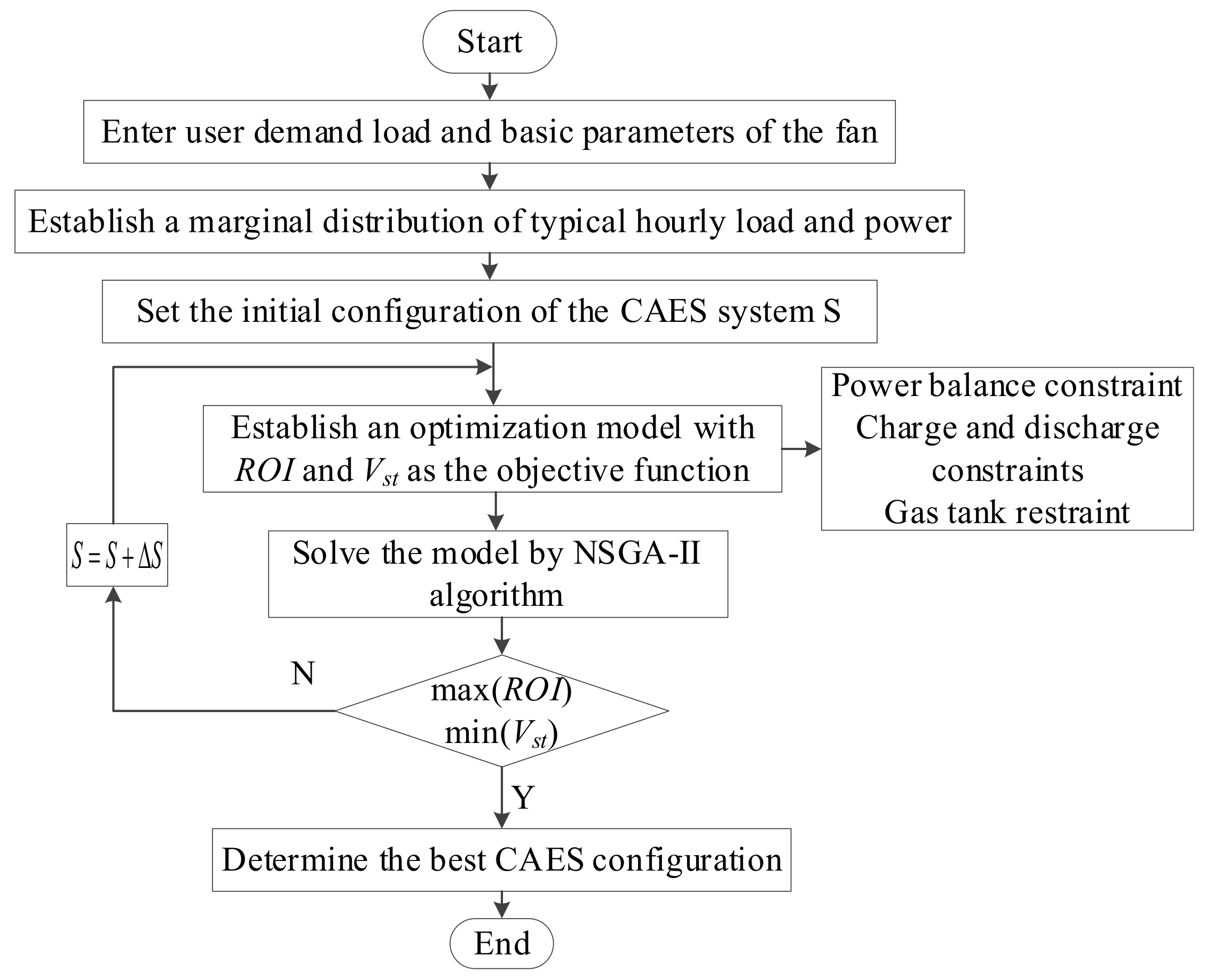
The CAES capacity optimization configuration model proposed in this section can be equivalent to a multi-objective optimization problem, which is solved by the NSGA-II algorithm [39] and can be effectively applied to various nonlinear and discrete practical problems. The algorithm flow chart is shown in Figure 10. The program uses MATLAB r2018b for coding, uses the NSGA-II algorithm as the optimization engine, and executes on a 2.5 GHz Intel Core i5-7300 HQ CPU and 8 GB RAM laptop.

The optimization variables are rated capacity and rated power, and the range is set according to the specific case. After the upper and lower limits of variables are calculated, a genetic algorithm can be used to search for optimization in this range with a certain step size. The optimization objective is the maximum return on investment and the minimum volume of the gas storage tank. The constraint conditions include power balance constraint, maximum gas and heat storage limit, and coupling limit of charge and discharge state. The solving principle of the algorithm is as follows. First, the operating mode of the wind turbine is optimized for different load scenarios. Subsequently, the capacity and power limit range of energy storage system are selected according to the power matching degree of wind power generator and user. Lastly, the optimal power and capacity configuration of the energy storage system is determined according to the optimization objectives and constraints. Some parameters of the algorithm were set as follows: population size 200, optimal individual coefficient 0.3, fitness deviation 1 × 10⁻¹⁰. Other initial conditions were set uniformly, as in Section 4.1.

4. Case Study

4.1. Simulation Parameter Settings

This study used typical hourly load and typical hourly wind as input parameters. Compared with the direct use of historical data averages, the experimental scheme produced data closer to the true value. At the same time, our approach was mainly from the perspective of the overall economic benefits of enterprise users and aimed to provide planning guidance for their project establishment. Therefore, the CAES system simulation scheme was adjusted for generality and universality, and the compression process and expansion process were equivalent to charging and discharging. The state was simulated, and it was assumed that the efficiency of the charging and discharging process was equivalent. The difference in the operating performance of the compression and expansion stages were not considered in detail, and is the focus of follow-up research. Based on the set conditions, the specific operating parameters of the compressed air energy storage system are shown in

Table 4. Economic and technical parameters of wind power coupled CAES system [3,30,43].

Kinds	Parameters	Value
Wind farm	Construction cost ICW ($/kW)	830
	Operating cost OMW ($/kWh-year)	0.0122
CAES	Installation cost Invp ($/kW)	700
	Installation cost InvC ($/kWh)	5
	Operating cost OMC ($/MWh-year)	200
	Life Lf (year)	20

and

Table 5. CAES structure technical parameters [30,33].

Kinds	Parameters	Value
General conditions	Ambient temperature (K)	298
	Ambient pressure (Pa)	1.013 × 105
	Gas constant (J/(kg∙K))	287.1
	Specific heat of air (J/(kg∙K))	1004
	Polytropic index	1.4
Compression section	Stage number	3
	Rated pressure ratio	3.7
	Efficiency	0.83
Expansion section	Stage number	3
	Rated pressure ratio	3.3
	Efficiency	0.85
Storage module	Ambient temperature	298
	Initial temperature	311
	pst,max/pst,min of storage chamber (MPa)	6.0/4.0
Others	Maximum heat storage capacity (MJ)	2 × 105
	Heat-exchange efficiency of heat exchanger	0.82
	Heat exchange medium specific heat	Water (4200)

. The other initial conditions included an investment interest rate of 8%, an average of 200 days of work per year within the useful life, 50% of the initial reserve status of the gas storage tank, and a limited capacity status range of 10% to 90%. $C_{CAES}^{rated}$ and $P_{CAES}^{rated}$ of the CAES system were set to discrete values within the range of (0, 12 MWh) and (0, 12 MW), with steps of 0.5 MWh and 0.5 MW for optimization [3] to configure the CAES system optimal storage scale. The grid electricity price [40] was taken from Shanxi province’s time-of-use dual pricing as shown in Figure 11. At present, many commercial CAES systems work under constant volume rings, that is, the storage pressure of the gas storage device has a constant volume and fluctuates within a certain range affected by the physical environment and working conditions. For example, the gas storage pressure of Huntorf in Germany is in the range of 4.3~7.0 MPa [41,42]. Considering the actual wind power output and user load demand, it was assumed that the gas storage pressure of the gas storage device fluctuated in the range of 4.0~6.0 MPa, and the pressure ratio of the compressor (expansion) was the same at each stage.

4.2. Multi-Scenario Analysis

4.2.1. Simulation Scene Settings

Considering that the average output power of FD70b wind turbines installed in the wind farm is only 791 kW per hour, and the factory load demand reached 3241 kW per hour, it is necessary to ensure that the wind farm maintains an appropriate number of wind turbines in normal operation to ensure power system balance. The number of fans configured can be solved by the following mathematical expression:

$$n_w=Roundup\left(\frac{P_{{}_L}^{ave}}{{\displaystyle \sum _{t=1}^{24}\left[P_W\left(t\right)\right]}/24}\right)$$

(41)

where n_w is the number of fans, Roundup is the round-up function, and $P_L^{ave}$ is the average hourly demand power of users.

For the above reasons, it is feasible to analyze the impact of wind turbine scale on system operation economy from time to time and determine a reasonable wind turbine scheduling strategy. Therefore, a variety of scenarios were set up to compare and select the scale of wind turbines suitable for wind farms. The scenario settings are shown in

Table 6. Scene setting.

Scenes	1	2	3	4
Wind Turbine	3	4	5	6
Actual power (MW)	2.373	3.164	3.955	4.746
Theoretical capacity (MWh)	4.5	6	7.5	9

.

4.2.2. Comparative Analysis under Multi-Scenario Operation

When the scale of the wind turbine on the power generation side changes, the operation of the wind power coupled CAES system changes accordingly. In scenario 1, the typical daily generation power of 56.98 MW is far from meeting the factory users’ daily average load power demand of 77.79 MW, and a daily load power shortage of 20.81 MW occurs. Figure 12 shows the improvement effect of the energy storage system on the power deficit of the client load. As can be seen from Figure 12, although the power deficit rate slows down by 6.17% under the action of the CAES system, the power deficit is still as high as 16.01 MW, which causes high power purchase costs, so this scheme is not feasible.

Table 7. Comparison of wind energy utilization on typical days.

Scenes		2	3	4
Power generation (MW)		75.97	94.96	113.95
Abandoned power (MW)	No CAES	7.97	20.67	36.77
	CAES	0.57	17.15	30.22
Abandonment rate (%)	No CAES	10.49	21.77	32.77
	CAES	0.75	18.06	26.52
Promote		9.74	3.71	5.75

shows wind energy utilization in scenarios 2 to 4. In scenario 2, the curtailment power of the wind farm with four wind turbines is 7.97 MW, and the load shortage power is 8.04 MW. The configuration of the CAES system can effectively reduce the curtailment power and improve the power shortage situation. The load shortage rate was changed from 10.34% to 3.10% and reduced by 7.24. At the same time, theoretically, the abandonment rate of wind farms can reach 0%. Under scenarios 3 and 4, it can be seen from Figure 12 that as the scale of wind turbines expands, the lack of power at the load decreases significantly, and the power shortage rate shows a downward trend. It should be noted that the number and scale of wind turbines increase, resulting in a high power abandonment rate. Although energy storage by CAES systems makes the energy utilization rate of wind farms increase to some extent, the power abandonment rate is still more than 15%, so this scheme has no prospect. In summary, for factory users with a total daily load power of 77.79 MW, it is feasible to adopt the scenario 2 configuration, which can reduce the curtailment rate by 9.74% and the power shortage rate by 7.24%. The next section considers the impact of Prated CAES and Crated CAES as optimization variables on system economy and power dispatch strategy under scenario 2 configurations.

4.3. Simulation Results

4.3.1. Analysis of Simulation Results

Under the constraints of the above initial parameters and constraints, combined with the power distribution data on the power generation side and the user side, the NSGA-II algorithm was used as the search engine to optimize the rated power and rated capacity of the system. Figure 13 is the optimal Pareto solution frontier of the model. As shown in Figure 13, it can be seen that when the energy storage configuration is within the range of the optimal solution set, the return on investment is maintained at more than 20.5%, but the volume scale of the gas storage tank is very different so a different capacity configuration plan for each energy storage system exists There are huge differences, and it is impossible to directly obtain the best energy storage planning plan for the wind turbine scale of scenario 2. Therefore, we introduced the TOPSIS [44] optimization method to select the optimal solution. The sample data were selected in the Pareto solution set as shown in

Table 8. Equipment configuration and evaluation indicators of each program.

Program	Optimal Sizing		ROI (%)	Vst (m3)	Edu (MWh)	Mre (kg)
	$P_{CAES}^{rated}$ (MW)	$C_{CAES}^{rated}$ (MWh)
Scaling			3	3	7	5
1	1	8	0.21851	1172.35	1243.96	2767.55
2	1	7	0.21724	1025.81	1243.96	2561.57
3	1	6	0.21597	879.26	1243.96	2355.58
4	1	5	0.21465	732.72	1240.69	2142.60
5	1	4.5	0.21337	659.45	1192.49	1936.62
6	1	3.5	0.21081	512.90	1050.77	1524.65
7	0.5	8	0.21978	1172.35	941.04	2623.36
8	0.5	7	0.218	1025.81	941.04	2425.58
9	0.5	6.5	0.21725	952.53	941.04	2322.58
10	0.5	5.5	0.21597	805.99	941.04	2116.60
11	0.5	4.5	0.21469	659.45	941.04	1910.61
12	0.5	4	0.21357	586.17	905.01	1730.63
13	0.5	3	0.21099	439.63	808.63	1318.66
14	0.5	2.5	0.20971	366.36	760.44	1112.68

. The evaluation indicators include the rate of return on investment (ROI), the volume of the gas storage tank (V_st), the amount of wind power consumed (E_du), and the reduction of carbon emissions (M_re), among which the newly introduced indicators mainly constrain the entire program from two aspects: environmental benefits and energy-saving benefits. The specific solving process includes the following steps. First, the original data matrix is normalized, and the weight coefficients of each index are evaluated. Then, the cosine method is used to find the ideal optimal solution and the ideal worst solution in the sample data, and calculate the degree of approximation of all samples to the ideal optimal solution ($D_i^{+}$), and the degree of approximation to the ideal worst solution (D_i). Finally, the closeness degree (C_i) between each evaluation scheme and the optimal scheme is calculated, the advantages and disadvantages of each scheme are evaluated based on this, and the optimal scheme is selected.

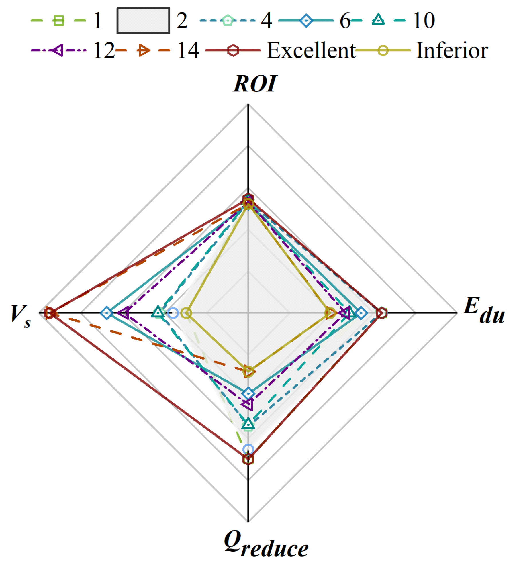
From the original sample data, the effect of CAES absorbing wind abandoning power tends to be gentle, which is the result of joint constraints of rated power and rated capacity of the energy storage system and wind power abandoning volume of wind farm. Carbon emission reduction has a great correlation with the volume of gas storage tanks and the power of energy storage system, and increases with increasing power and volume. For schemes 1 to 6 in Table 8, the rated power is 1 MW. Affected by the change of the upper limit of the power constraint, the overall carbon emission reduction is more than 100 kg higher than for schemes with a rated power of 0.5 MW under the same gas storage capacity. At the same time, when the rated power is 1 MW, the maximum amount of wind abandoning power that can be absorbed by CAES system is 1243.96 MWh. When the rated power is 0.5 MW, the maximum amount of wind abandoning power can be absorbed as 941.04 MWh. After normalized processing of sample data, we obtained a radar chart of four technical and economic indicators as shown in Figure 14, which vividly reflects the advantages and disadvantages of each sampling scheme under the multi-technical indicator evaluation system. Limited by the scope of the map, only part of the scheme is shown, such as scheme 1, scheme 2, the ideal best scheme and the ideal worst scheme. As shown in Figure 14, after the optimization of the NSGA-II algorithm, the ROI of each energy storage configuration scheme reached the optimal range. However, the V_st index is inversely related to E_du and M_re index, in that the scheme closer to the optimal range of V_st index is farther from the optimal range of E_du and M_re index. Therefore, how to use a reasonable evaluation method to measure the relationship between evaluation indicators is important.

The main purpose of this study was to use the energy storage system to realize peak cutting and valley filling of the new energy system, and to improve the utilization rate of random renewable energy. In the optimization of the NSGA-II algorithm, the two indexes of return on investment and volume of gas storage tank were analyzed. Therefore, on the premise that economic benefits can be effectively guaranteed, the consumption of wind power and carbon emission reduction should occupy a higher proportion in the evaluation system. Based on the above considerations, the APH analytic hierarchy process was used to re-determine the weight during TOPSIS optimization. The weights are shown in Table 8.

The TOPSIS optimization results are shown in

Table 9. TOPSIS evaluation results.

Program	${\mathit{D}}_{\mathit{i}}^{+}$	${\mathit{D}}_{\mathit{i}}^{-}$	Ci	Sort
1	0.1309	0.1297	0.4976	5
2	0.1189	0.1222	0.5067	1
3	0.1138	0.1137	0.4996	4
4	0.1118	0.1065	0.4880	7
5	0.0987	0.1007	0.5052	2
6	0.0982	0.0948	0.4911	6
7	0.1413	0.0959	0.4042	9
8	0.1347	0.0851	0.3873	12
9	0.1311	0.0802	0.3795	13
10	0.1227	0.0730	0.3731	14
11	0.1120	0.0735	0.3963	11
12	0.1113	0.0744	0.4007	10
13	0.1192	0.1003	0.4569	8
14	0.1297	0.1309	0.5024	3

. A change of C_i in the table is observed. The energy effective utilization rate of CAES system is limited due to the restriction of power upper limit, so the overall closeness of Program 7–13 is small. Due to the minimum gas storage scale of the CAES system and low investment cost, the degree of proximity of Program 14 was significantly improved. It can be seen that with the increase of the capacity and power of the energy storage system, the overall trend of the energy storage configuration scheme becomes closer and closer to the ideal and optimal scheme; however, the change in environmental benefits should also be reasonably evaluated. The change of proximity between each scheme and the optimal scheme further verifies the rationality of the aim of this paper. Therefore, the following conclusions can be drawn: Under various constraints, the energy storage scale configuration of scheme 2 is optimal; Only when the gas storage tank volume is controlled within a reasonable range can the entire energy storage configuration be optimized, rather than the situation in which the closer the gas storage scale is to the upper and lower limits, the better the optimization effect.

Figure 15 shows three different indicators for verifying and evaluating the feasibility of Scheme 2, namely the test results of the cumulative cash flow, investment payback period, and average annual net present value. As shown in the figure, if the energy storage configuration scheme is implemented, the system investment payback period is about 5 years, further verifying the economic value of the program.

4.3.2. System Most Scheduling Analysis

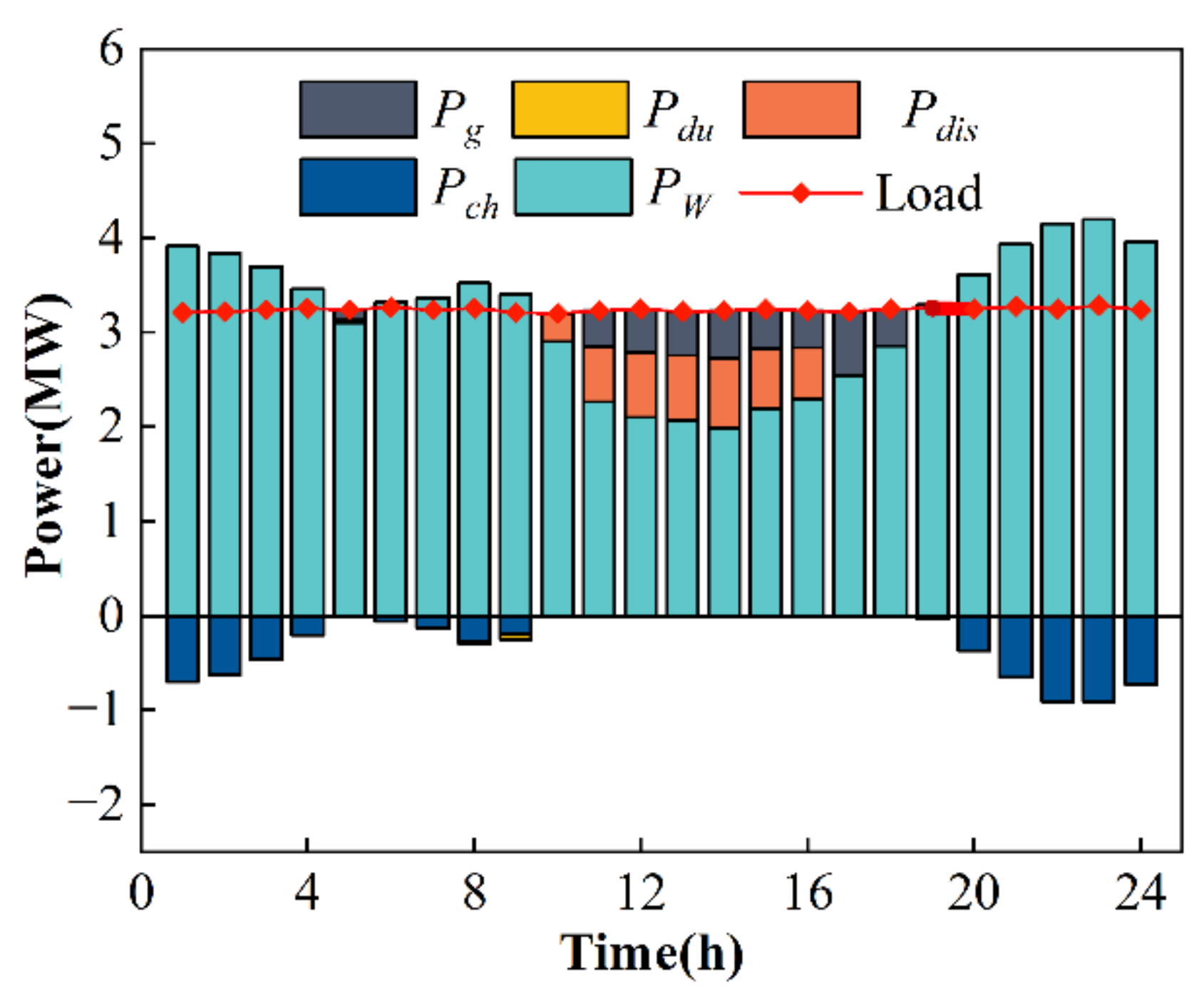
Under scheme 2, the energy storage configuration of the rated power is 1 MW and the rated capacity is 7 MWh, which can reduce carbon emissions by 2561.57 kg and consume 1243.96 MWh of curtailed wind power each year. The power dispatch situation is shown in Figure 16, where the charging power is positive and the discharge power is negative. In the entire energy system, the CAES system achieves the function of eliminating peaks and filling valleys. The specific performance is as follows. On the one hand, the conversion and storage of abandoned wind energy is controlled within the time scale. On the other hand, the power distribution of the energy storage system is adjusted under the grid time-of-use tariff policy; that is, the energy is stored when the electricity price is low. Electricity is sold when electricity prices are high to achieve peak divestiture. As showed in the figure, from 0:00 to 4:00, and 20:00 to 24:00, the wind is relatively high at night, and the CAES system is required to adjust energy storage to reduce the wind power curtailment rate. At the same time, considering that the grid electricity price is in the low stage during this period, the storage of excess wind is more economical, so the CAES system is mainly charging. The wind output from 9:00 to 19:00 cannot fully meet the load demand. Due to the influence of the electricity price of the power grid, this part of the load demand is mainly met by the discharge of the CAES system and supplemented by the power grid purchase. After11 h, the price of power grid sales fell, and the proportion of power grid purchases increased accordingly. It should be noted that after 5 h, the electricity price of the grid was at a trough, so the power dispatching of this part was mainly the power grid. As mentioned above, under the influence of time-of-use electricity prices, the CAES system can freely carry out storage of excess wind power and the transfer of load demand. When the optimization model evaluates its loss of profit, it increases the release of energy storage or increases purchase from the grid.

Under this optimization model, the energy changes in the gas storage tank after the wind power coupled CAES system runs for 24 h, as shown in Figure 17. The charging stage is divided into two stages: 0~5 h and 19~24 h. At 0~9 h, the power drops step by step from 0.70 MW to 0 MW and then rises to 0.18 MW. Although the power fluctuates in this stage due to the discharge condition, the gas storage in the gas storage tank shows an overall upward trend. The gas storage capacity of the gas storage tank finally reaches the maximum value of 80.6% within the operation cycle from 50%, with a total charge of about 2.62 MWh. In the discharge stage, the system discharges within 9~18 h, the discharge power varies in the range of 0~1 MW, and the gas storage capacity decreases step by step from the peak to 10%. After 24 h of wind power-coupled CAES system operation, the gas storage capacity of the gas storage tank is still 52.69%, which is within the limited range of storage scale of the gas storage device, ensuring the periodic and reusable function of the energy storage system and verifying the reliability of the optimization model.

Compared with the traditional CAES system, the adiabatic compressed air energy storage system effectively uses the heat generated in the compression process in the expansion process, which improves the efficiency of the whole energy storage and energy release process.

Table 10. TOPSIS evaluation results.

Flow	Switch	Temperature (K)
		HE1	HE2	HE3	HE4	HE5	HE6
Air	Inlet	461	506	519	311	259	265
	Outlet	327	335	337	405	397	397
Thermal fluid	Inlet	298	298	298	412	412	412
	Outlet	389	414	421	348	322	319

shows the temperature changes of the fluid in the heat exchanger at all levels when the first expansion is reached after the compression process. In the HE1~HE3 stages of heat exchange, heat carrying fluid plays a role in heat storage, and the inlet temperature is stable at 298 K. In the HE4~HE6 stages of heat exchange, heat carrying fluid has a heat release effect, and the inlet temperature is maintained at 412 K under the influence of the heat storage device. At the same time, it can be seen from the data in the table that under the energy storage capacity configuration scheme 2, the compressed air energy storage system can effectively meet the thermal load requirements of the whole energy storage and energy release link. Figure 18 shows the heat fluctuation in the heat reservoir during the day. In the compression process, the compression heat is stored in the heat reservoir. In the expansion process, the heat reservoir releases heat to improve the expansion efficiency. It is worth noting that at 14.5~16 h, the heat storage of the heat reservoir is exhausted, and the heat release process stops. At the end of the day, the heat storage of the heat reservoir reaches the maximum value of 1.1 × 10⁴ MJ, which meets the limit of the heat storage upper limit of the heat reservoir and reserves energy for the operation of the energy storage system the next day.

In summary, for the scale of wind turbines under scenario 2, the CAES system energy storage configuration of scenario 2 is the best. The optimization results of power balance are shown in Figure 19. During the 0–4 h and 6–9 h and 19–24 h periods, surplus wind appears after user load demand is met, so the CAES system is used for storage to reduce energy waste. Starting from 10 h, the wind weakens, and the wind power generation, compressed air energy storage, and power grid work together to supply power to the user. After 17 h, due to the impact of gas storage tank exhaustion, the power grid is mainly used to make up for the client’s load demand. Because the excess wind power in the wind power plant happens to be within the scheduling scope of the energy storage system, the CAES system can theoretically achieve 100% energy recovery and utilization under this energy storage configuration. It can be seen that under the action of a wind power-coupled CAES system, the whole power cycle system can effectively balance the random characteristics of the generating side and the user side and improve the utilization rate of new energy, which is of great research significance.

4.4. Visualization of CAES Capacity Configuration

In order to realize the visualization of the capacity configuration process of a compressed air energy storage system, this section describes a web-based simulation process. including a web-based software platform, data processing of renewable energy and load demand power under typical working conditions, capacity configuration planning of the energy storage system, and interconnection of processes such as multi-energy efficiency evaluation index scheme evaluation. The purpose is to consider the establishment of energy storage projects for new energy power generation companies, to accelerate the development of the green energy field.

4.4.1. Interface Function Design

(1)

Programming language

The web interface was developed using Html5 hypertext editing language, CSS, JavaScript and MATLAB APP designer. The server mainly adopts the MATLAB Web App Server platform.

(2)

Interface structure

The whole software is a multi-layer structure. The basic layout is as follows:

The first interface includes the two functions of registration and login; both have their own pages and judge whether a user can enter the platform through the user database.

Function selection interface: Jump to enter after successful login, including wind, photovoltaic, load data processing direction and traditional, adiabatic, isothermal and other compressed air energy storage system capacity configuration directions, as shown in Figure 20.

Operational level. This level is a numerical calculation interface. Both the data processing direction and the capacity configuration direction include the following modules. Input: including importing excel data, txt data and input boundary conditions. Output: generating images, tables, and exporting the corresponding data to display the calculation results.

(3)

Preset function

Data processing, including outlier elimination and extraction of typical operating conditions.

Capacity configuration. First, import parameters such as the power output of the power plant, the real-time electricity price of the power grid company, and the load demand of factory users. Then, determine the boundary conditions and select an appropriate algorithm. Finally, solve the capacity configuration and power dispatching strategy of the energy storage system in the corresponding scenario.

4.4.2. Example Demonstration

The energy storage capacity planning interface is shown in Figure 21. The entire interface is roughly divided into the boundary condition setting area, input parameter setting area, optimization result display area, and operation function selection area. Its functions are described below.

Boundary condition setting area. Adjust the number of power units in operation and the specification range of the energy storage system to simulate different application scenarios.

Input parameter setting area. Input parameters include renewable energy output power, load demand and local electricity price, which are obtained through the data processing module. At the same time, the above data can be imported into the platform by clicking the button. The right side of the button displays whether the operation is completed. After the confirmation button is pressed, the process is completed.

Optimization result display area. After the boundary conditions and input parameters are determined, click the Run button, and the optimization result display area displays the results of this operation employing numerical values and images.

Running function selection area. Three buttons are used for run, stop and return. The upper right corner includes the indicator light and the running status display box. The green light on the prompt box indicates that the system is working, and the red light indicates an error.

The above only shows part of the interface. Part of its code is shown in Appendix A.

5. Conclusions

To improve the volatility of wind power generation and the uncertainty of user demand, an adiabatic compressed air energy storage system is introduced to improve energy utilization. However, changes in the gas storage scale of energy storage systems often bring huge investment costs to power generation companies. Therefore, to reduce the burden on enterprise users and improve the economic value of the energy storage system, we provide a new method for energy storage planning. At the same time, an optimization model to maximize the return on investment and minimize the volume of the gas storage tank is established. The solving process is as follows. NSGA-II is used to solve the Pareto solution set of optimal storage scale of CAES system. Then, the optimal energy storage configuration scheme under current conditions is solved by the TOPSIS joint APH optimization method. Finally, the power dispatching strategy is determined to realize the production, distribution, storage and conversion between electric energy and wind energy. At the same time, the established model can be used to simulate and verify the operation of different wind power generation scales. The following conclusions were obtained.

(1)

In each operation cycle, the number of wind turbines in operation affects the economic benefits of the entire system. If the number is too small, the power output is insufficient, increasing the power shortage rate of the system. When the number is too large, although the power shortage rate of the system begins to decrease, the investment cost and discard wind power increases. Based on comprehensive analysis, the user of this plant chooses four fans to operate in conjunction with the CAES system, and the economic benefits are the best.

(2)

An A-CAES system with a rated power of 1 MW and a rated capacity of 7 MWh can meet the power demand of factory users with a typical hourly load power of 3.241 MW. The economic benefits are as follows include return on investment of 21.72%, the net present value is 1683 k$, the payback period is 4.8 years, and the scale of the gas storage device is only 1026 m3. The environmental benefits include effective consumption of 1244 MWh of abandoned wind power every year and reduced carbon emissions by 2562 kg.

(3)

The compressed air energy storage system capacity configuration program was established using MATLAB, and its interface includes a login registration page, a function selection page, a data processing page, and an energy storage capacity planning page. After a simulation case data test, it was found that the program ran reliably, and the visualization effect of the simulation process was obvious.

This study proposes a new method of optimal configuration of the CAES system scale to improve the uncertainty of wind and load demand and provides a new idea for the rationalization of power dispatch.

References

- Metal News. Wind Energy Beijing Declaration to develop 3 billion wind power, leading green development and implementing the "30·60" target. In Proceedings of the 2020 Beijing International Wind Energy Conference, Beijing, China, 14–16 October 2020; pp. 34–35. [Google Scholar]
- Roy, A.; Kedare, S.B.; Bandyopadhyay, S. Optimum sizing of wind-battery systems incorporating resource uncertainty. Appl. Energy 2010, 87, 2712–2727. [Google Scholar] [CrossRef]
- Xia, S.; Chan, K.W.; Luo, X.; Bu, S.; Ding, Z.; Zhou, B. Optimal sizing of energy storage system and its cost-benefit analysis for power grid planning with intermittent wind generation. Renew. Energy 2018, 122, 472–486. [Google Scholar] [CrossRef]
- Rehman, S.; Al-Hadhrami, L.M.; Alam, M.M. Pumped hydro energy storage system: A technological review. Renew. Sustain. Energy Rev. 2015, 44, 586–598. [Google Scholar] [CrossRef]
- Barbour, E.; Pottie, D.L. Adiabatic compressed air energy storage technology. Joule 2021, 5, 1914–1920. [Google Scholar] [CrossRef]
- Keck, F.; Lenzen, M.; Vassallo, A.; Li, M. The impact of battery energy storage for renewable energy power grids in Australia. Energy 2019, 173, 647–657. [Google Scholar] [CrossRef]
- Andersson, J.; Grönkvist, S. Large-scale storage of hydrogen. Int. J. Hydrogen Energy 2019, 44, 11901–11919. [Google Scholar] [CrossRef]
- Kale, V.; Secanell, M. A comparative study between optimal metal and composite rotors for flywheel energy storage systems. Energy Rep. 2018, 4, 576–585. [Google Scholar] [CrossRef]
- Berrada, A.; Loudiyi, K. Operation, sizing, and economic evaluation of storage for solar and wind power plants. Renew. Sustain. Energy Rev. 2016, 59, 1117–1129. [Google Scholar] [CrossRef]
- Barbour, E.; Mignard, D.; Ding, Y.; Li, Y. Adiabatic Compressed Air Energy Storage with packed bed thermal energy storage. Appl. Energy 2015, 155, 804–815. [Google Scholar] [CrossRef] [Green Version]
- Díaz-González, F.; Sumper, A.; Gomis-Be Llmunt, O.; Villafáfila-Robles, R. A review of energy storage technologies for wind power applications. Renew. Sustain. Energy Rev. 2012, 16, 2154–2171. [Google Scholar] [CrossRef]
- Jannelli, E.; Minutillo, M.; Lavadera, A.L.; Falcucci, G. A small-scale CAES (compressed air energy storage) system for stand-alone renewable energy power plant for a radio base station: A sizing-design methodology. Energy 2014, 78, 313–322. [Google Scholar] [CrossRef]
- Razmi, A.R.; Afshar, H.H.; Pourahmadiyan, A.; Torabi, M. Investigation of a combined heat and power (CHP) system based on biomass and compressed air energy storage (CAES). Sustain. Energy Technol. Assess. 2021, 46, 101253. [Google Scholar] [CrossRef]
- Sun, H.; Luo, X.; Wang, J. Feasibility study of a hybrid wind turbine system–Integration with compressed air energy storage. Appl. Energy 2015, 137, 617–628. [Google Scholar] [CrossRef] [Green Version]
- Venkataramani, G.; Ramakrishnan, E.; Sharma, M.R.; Bhaskaran, A.H.; Dash, P.K.; Ramalingam, V.; Wang, J. Experimental investigation on small capacity compressed air energy storage towards efficient utilization of renewable sources. J. Energy Storage 2018, 20, 364–370. [Google Scholar] [CrossRef]
- Odukomaiya, A.; Kokou, E.; Hussein, Z.; Abu-Heiba, A.G.; Graham, S.D.; Momen, A.M. Near-isothermal-isobaric compressed gas energy storage. J. Energy Storage 2017, 12, 276–287. [Google Scholar] [CrossRef]
- Cárdenas, B.; Pimm, A.J.; Kantharaj, B.; Simpson, M.C.; Garvey, J.A.; Garvey, S.D. Lowering the cost of large-scale energy storage: High temperature adiabatic compressed air energy storage. Propuls. Power Res. 2017, 6, 126–133. [Google Scholar] [CrossRef]
- Alirahmi, S.M.; Mousavi, S.B.; Razmi, A.R.; Ahmadi, P. A comprehensive techno-economic analysis and multi-criteria optimization of a compressed air energy storage (CAES) hybridized with solar and desalination units. Energy Convers. Manag. 2021, 236, 114053. [Google Scholar] [CrossRef]
- Zhang, Y.; Xu, Y.; Guo, H.; Zhang, X.; Guo, C.; Chen, H. A hybrid energy storage system with optimized operating strategy for mitigating wind power fluctuations. Renew. Energy 2018, 125, 121–132. [Google Scholar] [CrossRef]
- Alirahmi, S.M.; Razmi, A.R.; Arabkoohsar, A. Comprehensive assessment and multi-objective optimization of a green concept based on a combination of hydrogen and compressed air energy storage (CAES) systems. Renew. Sustain. Energy Rev. 2021, 142, 110850. [Google Scholar] [CrossRef]
- Razmi, A.R.; Soltani, M.; Ardehali, A.; Gharali, K.; Dusseault, M.; Nathwani, J. Design, thermodynamic, and wind assessments of a compressed air energy storage (CAES) integrated with two adjacent wind farms: A case study at Abhar and Kahak sites, Iran. Energy 2021, 221, 119902. [Google Scholar] [CrossRef]
- Jani, V.; Abdi, H. Optimal allocation of energy storage systems considering wind power uncertainty. J. Energy Storage 2018, 20, 244–253. [Google Scholar] [CrossRef]
- Dvorkin, Y.; Ricardo, F.; Wang, Y.; Xu, B.; Kirschen, D.; Pandzic, H.; Watson, J.P.; Silva-Monroy, C.A. Co-planning of Investments in Transmission and Merchant Energy Storage. IEEE Trans. Power Syst. 2017, 33, 245–256. [Google Scholar] [CrossRef]
- Bina, V.T.; Ahmadi, D. Stochastic modeling for scheduling the charging demand of EV in distribution systems using copulas. Int. J. Electr. Power Energy Syst. 2015, 71, 15–25. [Google Scholar] [CrossRef]
- IEC 61400-12-1-2017; Wind Turbines Generator Systems-Part 12-1: Power Performance Measurements of Electricity Producing Wind Turbines. International Electrotechnical Commission: Geneva, Switzerland, 2017. Available online: https://webstore.iec.ch/publication/26603 (accessed on 15 February 2022).
- Wang, X.; Wang, Z. Wind turbine wind speed-power data cleaning based on improved bin algorithm. J. Intell. Sci. Technol. 2020, 2, 62–71. [Google Scholar] [CrossRef]
- Xiang, L.; Jie, G. Using the Clustering Algorithm Forecast in the Power Grid Typical Daily Load Curve. Power Energy 2013, 34, 47–50. [Google Scholar] [CrossRef]
- Zhang, B.; Zhuang, C.; Jun, H.U.; Chen, S.; Zhang, M.; Wang, K.; Zeng, R. Ensemble Clustering Algorithm Combined with Dimension Reduction Techniques for Power Load Profiles. Proc. CSEE 2015, 35, 3741–3749. [Google Scholar] [CrossRef]
- Xiaoqing, X.; Wei, T.; Jian, M. Typical load curve extraction method for energy storage capacity configuration. Acta Sol. Energy 2018, 39, 2234–2242. [Google Scholar]
- Wang, H.; Zhang, C.; Li, K.; Ma, X. Game theory-based multi-agent capacity optimization for integrated energy systems with compressed air energy storage. Energy 2021, 221, 119777. [Google Scholar] [CrossRef]
- Ma, X.; Zhang, C.; Li, K.; Li, F.; Wang, H.; Chen, J. Optimal dispatching strategy of regional micro energy system with compressed air energy storage. Energy 2020, 212, 118557. [Google Scholar] [CrossRef]
- Tong, Z.; Cheng, Z.; Tong, S. A review on the development of compressed air energy storage in China: Technical and economic challenges to commercialization. Renew. Sustain. Energy Rev. 2021, 135, 110178. [Google Scholar] [CrossRef]
- Wu, C.; Chen, Z.; Zhang, J.; Zhang, X.; He, Z. Wind power system cost/power supply reliability evaluation considering advanced adiabatic compressed air energy storage. Electr. Power Autom. Equip. 2020, 40, 62–75. [Google Scholar] [CrossRef]
- Chen, J.; Liu, W.; Jiang, D.; Zhang, J.; Ren, S.; Li, L.; Li, X.; Shi, X. Preliminary investigation on the feasibility of a clean CAES system coupled with wind and solar energy in China. Energy 2017, 127, 462–478. [Google Scholar] [CrossRef]
- Wei, X.H.; Zhou, H. Evaluating the Environmental Value Schedule of Pollutants Mitigated in China Thermal Power Industry. Res. Environ. Sci. 2003, 16, 53–56. [Google Scholar] [CrossRef]
- Xiaoqing, X. Research on Energy Storage System Capacity Optimization Configuration and Life Cycle Economic Evaluation Method; China Agricultural University: Beijing, China, 2018. [Google Scholar]
- Yan, S.; Maolin, C. Working characteristics of two kinds of air-driven boosters. Energy Convers. Manag. 2011, 52, 3399–3407. [Google Scholar] [CrossRef]
- Cai, M.; Kawashima, K.; Kagawa, T. Power Assessment of Flowing Compressed Air. J. Fluids Eng. 2006, 128, 402–405. [Google Scholar] [CrossRef]
- Wang, X.; Cheng, Y.; Huang, M.; Ma, H. Multi-objective optimization of a gas turbine-based CCHP combined with solar and compressed air energy storage system. Energy Convers. Manag. 2018, 164, 93–101. [Google Scholar] [CrossRef]
- Polaris Sells Power Grid. 2021 National New Electricity Price Panorama. 2020. Available online: https://www.163.com/dy/article/FUKQMO9005509P99.html (accessed on 24 December 2020).
- Yang, Q.; Liu, G.; Zhao, Y.; Li, L. Study on the working characteristics of compressed air energy storage system. Fluid Mach. 2013, 41, 14–24. [Google Scholar] [CrossRef]
- Li, L.; Liang, W.; Lian, H.; Yang, J.; Dusseault, M.B. Compressed air energy storage: Characteristics, basic principles, and geological considerations. Adv. Geo Energy Res. 2018, 2, 135–147. [Google Scholar] [CrossRef] [Green Version]
- Nourai, A. Installation of the First Distributed Energy Storage System (DESS) at American Electric Power (AEP); Sandia National Laboratories (SNL): Albuquerque, NM, USA; Livermore, CA, USA, 2007. [Google Scholar] [CrossRef] [Green Version]
- You, T.; Fan, Z. A TOPSIS method for interval number multiple attribute decision making. J. Northeast. Univ. 2005, 26, 798–800. [Google Scholar] [CrossRef]
Figure 1.
Structure diagram of wind power coupled CAES system.
Figure 2.
Real-time wind speed of wind farm.
Figure 3.
Wind speed distribution probability map (00:00–1:00).
Figure 4.
Wind turbine output characteristics.
Figure 5.
Typical hour fan output power curve.
Figure 6.
Plant load demand power curve from 1–5 August.
Figure 7.
Load demand power probability distribution (00:00–1:00).
Figure 8.
Typical hourly load demand curve.
Figure 9.
Working diagram of wind power coupled CAES system.
Figure 10.
Flow chart for determining the best CAES storage scale.
Figure 11.
Time-of-use electricity price.
Figure 12.
Daily load lack power change.
Figure 13.
Pareto optimal frontier.
Figure 14.
Radar chart of partial project evaluation results.
Figure 15.
Cumulative cash flow, ROI, NPV of the wind power coupled CAES system.
Figure 16.
Wind power coupled CAES system daily power dispatch.
Figure 17.
SOC change curve during charging and discharging.
Figure 18.
TES heat storage curve.
Figure 19.
Power balance optimization results.
Figure 20.
Schematic diagram of function selection.
Figure 21.
Schematic diagram of the capacity planning interface of adiabatic CAES system.