Article

Multi-Objective Dynamic Economic Emission Dispatch with Electric Vehicle–Wind Power Interaction Based on a Self-Adaptive Multiple-Learning Harmony-Search Algorithm

1
School of Electronic and Information Engineering, Zhongyuan University of Technology, Zhengzhou 450007, China
2
Guangzhou Institute of Technology, Xidian University, Xi’an 710071, China
3
Guangdong Power Grid Co., Ltd., Guangzhou 510000, China
*
Authors to whom correspondence should be addressed.
Submission received: 30 May 2022 / Revised: 30 June 2022 / Accepted: 4 July 2022 / Published: 6 July 2022

Abstract

:
Dynamic economic emission dispatch (DEED) in combination with renewable energy has recently attracted much attention. However, when wind power is considered in DEED, due to its generation uncertainty, some additional costs will be introduced and the stability of the dispatch system will be affected. To address this problem, in this paper, the energy-storage characteristic of electric vehicles (EVs) is utilized to smooth the uncertainty of wind power and reduce its impact on the system. As a result, an interaction model between wind power and EV (IWEv) is proposed to effectively reduce the impact of wind power uncertainty. Further, a DEED model based on the IWEv system ( DEED IWEv ) is proposed. For solving the complex model, a self-adaptive multiple-learning multi-objective harmony-search algorithm is proposed. Both elite-learning and experience-learning operators are introduced into the algorithm to enhance its learning ability. Meanwhile, a self-adaptive parameter adjustment mechanism is proposed to adaptively select the two operators to improve search efficiency. Experimental results demonstrate the effectiveness of the proposed model and the superiority of the proposed method in solving the DEED IWEv model.

1. Introduction

With the rapid development of society and the economy, the demand for electric energy is also rising rapidly. Meanwhile, the electric power industry is strictly controlled by the government for energy-saving and emission reduction. In this context, it is crucial to optimize the operation of the power system by scheduling the generator outputs according to the predicted load demands over a certain period to reduce, simultaneously, fuel costs and pollution emissions. Therefore, dynamic economic emission dispatch (DEED) has attracted much attention due to its practical nature and because it is more in line with the actual short-term load demands.
A typical DEED problem is a multi-objective optimization problem that generally aims to minimize the fuel costs and the pollution emissions simultaneously. Moreover, several practical constraints should be considered at the same time when optimizing the two objectives, such as power balance constraints, ramp rate limits, output power constraints, spinning reserve constraints, etc. The DEED model is not only suitable for dynamically dispatching the generator outputs of the system according to the different load demands at a certain interval [1], but also accords with the dynamic properties of EV charging and discharging behaviors and the uncertainty of wind power. Therefore, the research of combining DEED and renewable energy has recently gained much interest.
As a renewable energy, wind power was introduced into the grid to reduce the generation of traditional thermal power units, thus reducing the consumption of fossil fuels and pollution emissions [2,3,4]. As for the existing literature on power dispatch with wind power generation, Liu et al. in [5] developed a load allocation model to consider the impact of wind power on emission control. Zhang et al. in [6] proposed a probability distribution model with a “generic distribution” to predict the wind power errors in economic dispatch problems. Hu et al. in [7] considered dynamic economic emission dispatch (DEED) with wind power under energy market reforms. Aghaei et al. in [8] proposed a scenario-based stochastic programming framework to model the stochastic nature of load demand. In [9], Jangir et al. proposed to solve the economic-emission constraint problem in wind power integrated systems using the grey wolf optimizer algorithm. Due to its uncertainty, when wind power generation exceeds the needs of the dispatching system, it will cause waste. When wind power generation is insufficient to meet the needs of the dispatching system, an additional spinning reserve from the system is required and some cost will be incurred. It is also worthwhile studying how to eliminate the additional costs caused by the uncertainty of wind power generation. Chen et al. [10] proposed a constrained multi-objective population extreme value optimization algorithm considering the uncertainty of wind power generation. Hagh et al. in [11] used the exchange market algorithm to solve the EED problem with wind farms. In [12], Jin et al. considered the factors that available wind power is both overestimated and underestimated, and proposed an EED model for to address this.
Moreover, with the rapid development of EVs, an increasing number of them are integrated into our life [13], and the vast number of EVs also impose a burden on the power grid. Still, a certain number of EVs can also be used as energy storage elements to reserve the power [14,15,16,17]. Researchers have added EVs to the grid in a V2G manner [18,19,20,21], but have not realized the dynamic management of EV charging and discharging, and have not truly integrated EVs to the DEED model. To address the uncertainty of wind power and take advantage of electric vehicles as energy storage elements, several studies were conducted combining EVs with wind power [22]. In [23], Qu et al. considered EVs and wind power generation in dynamic power dispatch using the MOEA/D algorithm. Zhang et al. in [24] combined EVs and wind power to develop a multi-objective hydrothermal wind power with the EV dispatch (MOHTWES) model. Zou et al. in [25] proposed a multi-objective virus colony search algorithm for optimizing dynamic economic and emission scheduling of EVs and wind power. The above studies combine EVs and wind power.
It follows from the above that current research analyzes the additional cost caused by wind power uncertainty, but does not provide a satisfactory solution to reduce such cost. Further, in these studies, the EVs and wind power are hybridized in a simple way and there is no actual interaction between them. Therefore, in this paper, we propose a model based on the interaction between wind power generation and EVs: when the generated wind power cannot meet the dispatch demand, the EV will discharge to compensate, and when the generated wind power exceeds the dispatch demand, the EV will be charged to absorb the excessive power. Further, a new DEED model based on the interaction between EVs, and wind power is proposed to reduce the additional cost of wind power. The proposed DEED IWEv model integrates two objective functions of cost and emission, and combines some equality and inequality constraints, such as the power balance constraint, owner travel constraint, spinning reserve constraint, and so on.
In recent years, swarm intelligence optimization algorithms were widely used to solve the practical optimization problem in many fields [26,27] because of their good global search and convergence performance and strong robustness. Meanwhile, such algorithms were also applied to solve the DEED problem. For example, Yan et al. in [1] developed a novel multi-objective pigeon-inspired optimization with double disturbance to solve the basic DEED problem. Basu et al. in [28] employed the particle swarm optimization algorithm to optimize the DEED. Jangir et al. in [9] used the grey wolf optimizer algorithm to solve the economic emission dispatch problem with the integration of wind power.
The proposed DEED IWEv model is a high-dimensional, strongly coupled, nonlinear, non-convex, and constrained multi-objective problem. To solve this complex problem, a new self-adaptive multiple-learning multi-objective harmony-search algorithm, termed SAMLHS is proposed. Two new learning operators, namely, elite-learning and experience-learning operators are introduced into the HS algorithm to enhance its global and local search abilities, respectively. In addition, a self-adaptive parameter-adjustment mechanism is proposed to adaptively select the two operators to improve the search efficiency of the population. In the experiments, we compare the proposed SAMLHS algorithm with six state-of-the-art algorithms and validate the proposed DEED IWEv model in different scenarios, while considering different confidence levels, different scales of EVs, and different wind powers. The results show that the proposed model and algorithm are reasonable and effective. The major contributions of this paper are as follows: (i) a new DEED model considering the interaction between EVs and wind power is proposed; (ii) a new self-adaptive multiple-learning multi-objective harmony-search algorithm is proposed to optimize the DEED IWEv problem; and (iii) numerous experiments are conducted to validate the correctness and effectiveness of the model and the algorithm. It can be concluded that the model and algorithm proposed in this paper provide a good framework and method for addressing the uncertainty of wind power generation.
The rest of the paper is organized as follows. Section 2 studies the modeling of DEED with the IWEv system. Section 3 describes in detail the proposed SAMLHS algorithm and its implementation in solving the model. The experiment settings, results, and discussion are presented in Section 4. The conclusions are given in Section 5.

2. Modeling of D E E D I W E v

This section describes the model in detail, and the parameters involved are described in Table 1.

2.1. Wind Power Modeling

The wind power output is determined by the stochastic wind speed [29,30,31], which is modeled using the widely used two-parameter Weibull distribution function. For each interval, the Cumulative distribution function (CDF) and Probability density function (PDF) of the wind speed is expressed as in the following two equations, respectively.
F ( v t ) = 1 e x p [ ( v t / c t ) k t ] , v t 0
f ( v t ) = ( k t / c t ) ( v t / c t ) k t 1 e x p [ ( v t / c t ) k t ] , v t 0
k t and c t are calculated by μ t and σ t ; the detailed calculation can be found in [32].
The active power of wind turbine P w . t and wind speed v t are related by:
P w . t = { 0 ,     v t < v i n   o r   v t v o u t   P r a t e v t v i n v r a t e v i n ,     v i n v t < v r a t e   P r a t e ,     v r a t e v t < v o u t  
The PDF of P w . t in the t th interval is derived by combining (2) and (3)
f ( P w . t ) = { k t ( v r a t e v i n ) p r a t e c t [ ( 1 + v r a t e v i n ) v i n c t ] k t 1 e x p { [ ( 1 + v r a t e v i n v i n p r a t e P w . t ) v i n c t ] k t } , 0 < P w . t < P r a t e 1 e x p [ ( v i n c t ) k t ] + e x p [ ( v o u t c t ) k t ] ,   P w . t = 0   e x p [ ( v r a t e c t ) k t ] e x p [ ( v o u t c t ) k t ] ,     P w . t = P r a t e  
Therefore, the CDF of wind power is also be defined by the discrete probability in (−∞, +∞), and can be derived by Equations (1) and (4), expressed as follows,
F ( P w . t ) =   Pr ( P w . t < P w . t ) =   { 0 ,     P w . t < 0 1 e x p { [ ( 1 + v r a t e v i n v i n p r a t e P w . t ) v i n c t ] k t } + e x p [ ( v o u t c t ) k t ] , 0 P w . t < P r a t e 1 ,   P w . t   P r a t e  

2.2. EV Dispatch Model

In this model, private vehicles and commuter vehicles are the main research objectives. Because most EVs are used for commuting, their travel time is mainly in the morning and evening, and they are immobile most of the time. When they are immobile, they can participate in grid dispatching by means of V2G. Note that it is not necessary to control the charging/discharging of each EV individually. The hierarchical dispatch model [23] is employed for the EVs, dividing EVs in the same area into several aggregates; these aggregates are controlled by the corresponding aggregation mechanism for charging and discharging. The charging and discharging states of the EVs are represented by a sign function at each dispatching interval:
{ P c h . t = s i g n ( x ) i = 1 N e P e . i ,   x < 0 P D c h . t   =   s i g n ( x ) i = 1 N e P e . i ,   x > 0 P c h . t   a n d   P D c h . t = 0 ,   x = 0
The description of EV charging and discharging states is shown in Table 2.

2.3. Interaction between Wind Power and EVs

Because wind power generation is uncertain, it is not always consistent with the demand of the dispatching system [23,32]. Therefore, an interaction model between wind power and EVs is proposed to reduce the impact of the uncertainty and is specified as follows.
When the available wind power produces too much, exceeding the demand of the dispatching system, wind power curtailment occurs. At this time, the EVs can absorb the surplus power by charging; however, the wind power may still exceed the amount that can be dispatched, i.e., P w . j . t > P c h . t + P w d i s . j . t . At this time, the abandoned wind power can be computed by
P w . c u r = t = 1 T j = 1 N w E c e   ( P w . j . t P c h . t P w d i s . j . t )
On the contrary, when the available wind power is insufficient, it cannot meet the demand of the dispatching system. In this case, the EVs are required to discharge to compensate for the gap. Nevertheless, the demand of the dispatching system may still not be met. The generated wind power is fully used at this time, and thus there is no curtailment required for the wind power, i.e., P w d i s . j . t > P D c h . t + P w . j . t . In this case, additional power is invoked from the reserve of the system, denoted as P w . n c u r , and can be calculated by
P w . n c u r = t = 1 T j = 1 N w E n c e   ( P w d i s . j . t P D c h . t P w . j . t )  
P w . j . t is a random variable in the range [ 0   P r a t e ] , and its change probability is determined by the PDF defined in Equation (4). E c e (∙) and E n c e (∙) are the expected values of the wind power curtailment and no curtailment occurring in the I W E v system, respectively. Detailed calculations for P w . c u r and P w . n c u r can be found in [32].

2.4. Objective Functions

System costs and pollutant emissions are both objective functions of the proposed DEED model with the interaction between wind power and EVs. Specifically, the total system cost is the sum of the fuel cost of the thermal power units, the direct cost of the wind power, and the interaction cost of the I W E v model, expressed as follows,
F C = F P + F W + F i n t
Fuel cost function: The fuel cost function considering the valve-point effect can be defined as the sum of the quadratic function and the sine function [33]:
F P = t = 1 T i = 1 N [ α i + β i P i . t + γ i P i . t 2 + | ζ i s i n { φ i ( P i m i n P i . t ) } | ]
F W is the direct wind power cost that can be expressed in terms of the dispatch wind power,
F W = t = 1 T i = 1 N w D j . t P w d i s . j . t
Interaction cost of the IWEv model: Based on the analysis in Section 2.3, the interaction cost can be divided into two parts corresponding to the two interaction scenarios considered in the model, respectively. Specifically, when the available wind power over-exceeds the system demand, and even the excessive power cannot be consumed by the EVs, a curtailment cost will be incurred. On the contrary, when the wind power cannot meet the system demand and the discharging of the EVs still cannot fill the gap, some extra spinning reserve is required and the corresponding cost is generated [34]. Here, both costs are collectively referred to as the interaction cost, which can be expressed as follows:
F i n t = t = 1 T j = 1 N w C c w j . t × P w . c u r + t = 1 T j = 1 N w C r w j . t × P w . n c u r  
Emissions are mainly caused by the process of thermal power generation, including C O x , S O x , and so on. The relationship between the emission and the active power of the units can be expressed as follows:
F M = t = 1 T i = 1 N [ ( a i + b i P i . t + c i P i . t 2 + d i exp ( e   i   P i . t )   ) ]

2.5. System Constraints

The following equality and inequality constraints are considered in the proposed DEED IWEv model.
System power balance constraints: In each interval, the sum of the total active power of thermal power units, EV charging or discharging power, and the wind power should satisfy the load demands and the system loss. P i . t and P w d i s . j . t should also meet the boundary limits.
t = 1 N P i . t + j = 1 N w P w d i s . j . t + P D c h . t = P D . t + P L . t + P c h . t
P i m i n P i . t P i m a x
0 P w d i s . j . t P r a t e
Note that P L . t is calculated using the B-coefficient method [35].
P L . t = t = 1 T i = 1 N P i . t B i j P j . t + i = 1 N P i . t B i 0 + B 00
Travel constraint of the EVs owners: The primary purpose of EVs is to meet the travel needs of their owners.
t = 1 T E c o n . t = t = 1 T C P c h . t t t = 1 T 1 D P D c h . t t
E c o n . t can be calculated as,
E c o n . t = E L
EVsremaining power constraint: The remaining power E t of the EVs at time t is defined as,
E t = E t 1 + C P c h . t t 1 D P D c h . t t E c o n . t  
Charging and discharging power constraints: The charging and discharging power of the EVs in each interval should meet the following limits:
{ | P c h . t | P R c h P D c h . t P R D c h
Ramp rate limits: The ramp rates of the thermal power units should satisfy the following inequality constraints:
{ P i . t P i . t 1 U R t t P i . t 1 P i . t D R t t
Spinning reserve constraints: To cope with the impact caused by EV charging/discharging and wind power uncertainties, the up and down spinning reserves must be considered in the model, modeled using the form of the chance-constraint expressed as:
Pr { i = 1 N min ( P i . t m a x P i . t , U R t 6 ) + ϑ u ( P D c h . t + P c h . t ) ω u P w . t S R . t u   0 } η 1
Pr { i = 1 N min ( P i . t P i . t m i n , D R t 6 ) + ϑ d ( P D c h . t + P c h . t ) ω d ( P r a t e P w . t ) 0 } η 2
Equations (23) and (24) can be transformed into a deterministic form by Equation (5) and then solved, expressed as Equations (25) and (26),
1 ω u   [ i = 1 N ( P i . t m a x P i . t ) + ϑ u ( P D c h . t + P c h . t ) S R . t u ] + v i n p r a t e v r a t e v i n   c t p r a t e v r a t e v i n | ln [ 1 η 1 + e x p ( ( v o u t c t ) k t ) ] | 1 / k t  
P r a t e 1 ω d   [ i = 1 N ( P i . t m a x P i . t ) + ϑ d ( P D c h . t + P c h . t ) ] + v i n p r a t e v r a t e v i n c t p r a t e v r a t e v i n | ln [ η 2 + e x p ( ( v o u t c t ) k t ) ] | 1 / k t
η 1 and η 2 represent the tolerance of the spinning reserve when the available wind power is insufficient for the dispatching demand. S R . t u is usually taken as 5–10% of load demand.

3. Self-Adaptive Multi-Learning Harmony-Search Algorithm and Its Implementation in the D E E D I W E v

In this section, the basic HSA and the proposed SAMLHS are introduced in detail. The procedure of SAMLHS and its implementation in solving the model are then given.

3.1. The Basic HSA

The HSA is a population-based intelligent optimization algorithm proposed by Geem and Kim [36] that imitates the process of musicians looking for harmony. When composing harmonies, musicians usually try to memorize the various possible combinations of tones in their memory stores. This process of finding the perfect harmony is similar to the process of finding the optimal solution to a practical problem. As a popular global optimization algorithm, the HSA has been utilized in the fields of function optimization, mechanical structure design, data classification system optimization, and so on [37]. The steps of the basic HSA are described as follows:
Step 1: Initialize the algorithm parameters and harmony memory (HM). Assign the predefined values to the following parameters: HM size (HMS), HM consideration rate (HMCR), pitch adjusting rate (PAR), bandwidth (bw), and the maximum number of function evaluations (Max_FEs). The initial population stored in HM can be generated by:
x i ,   j = L B j + r a n d · ( U B j L B j )   j = 1 ,   2 ,   , d
where r a n d [ 0 ,   1 ] , U B j and L B j are, respectively, the upper and lower bounds of the j th dimension of the decision variables. d is the variable dimension.
Step 2: Improvise new solutions. A new harmony solution x n e w = ( x n e w ,   1 ,   x n e w ,   2 , , x n e w ,   n ) is created. The detailed improvision procedure is described in Algorithm 1.
Algorithm 1. The procedure of improvisation in HSA.
1. for j = 1   t o   d
2.       if r a n d < H M C R
3.         x n e w ,   j   { x 1 , j ,   x 2 , j , ,   x H M S , j j     }   / /   m e m o r y     c o n s i d e r a t i o n
4.             if r a n d < P A R
5.                    x n e w ,   j = x n e w ,   j + b w   / /   p i t c h   a d j u s t m e n t
6.             end if
7.         else
8.                 x n e w ,   j = L B j + r a n d · ( U B j L B j )   / /   r a n d o m i z a t i o n
9.       end if
10.end for
Step 3: Update the harmony memory. The HM will be updated if the fitness value of the newly generated harmony vector is better than that of the worst one in the HM.
Step 4: Repeat Steps 2–3 until Max_FEs is reached.

3.2. The Proposed SAMLHS Algorithm

The basic HSA only uses two simple parameters to control the generation of new individuals throughout the whole evolutionary process. It lacks control over the evolutionary process and cannot guide the evolution of individuals according to the different search needs at different evolutionary stages. Therefore, search efficiency and convergence speed cannot be ensured. In addition, in the basic HSA, the individuals only learn from the HM, while the search experience of the global optimal solution and other individuals is not extracted and learned sufficiently. It is, therefore, easy to fall into the local optimum, and the solution quality cannot be ensured. Further, the DEED problem to be solved is a high-dimensional, nonlinear, strongly coupled, and constrained multi-objective problem, which may be a great challenge to the basic HSA. Therefore, this paper proposes a novel self-adaptive multiple-learning harmony-search algorithm to solve the complex DEED IWEv .

3.2.1. Self-Adaptive Parameter Adjustment

As shown in Algorithm 1, in the basic HSA, the two updating methods (shown in Lines 3 and 8, respectively) are selected with a fixed probability HMCR in the iteration process. Once the population has been trapped into a local optimum, it is hard for the algorithm to jump out of the local region when the HMCR is large. Conversely, when the HMCR is small, it is hard for the population to converge. Even though the HMCR is set to a median, its search efficiency and convergence speed may be not satisfactory. Thus, it can be concluded that the basic HSA is sensitive to the value of HMCR and thus the parameters should be elaborately controlled to ensure the performance of the algorithm.
A self-adaptive parameter adjustment mechanism is, therefore, proposed to adaptively control the two parameters HMCR and PAR according to the current number of function evaluations (FEs), which can be expressed as follows:
H M C R = H M C R m i n + ( H M C R m a x H M C R m i n ) × e ( 2 × F E s M a x _ F E s )
P A R = P A R m i n + ( P A R m a x P A R m i n ) × e ( 2 × M a x F E s F E s M a x _ F E s )
where H M C R m i n and H M C R m a x are, respectively, the minimum and maximum of HMCR and P A R m i n and P A R m a x are, respectively, the minimum and maximum of PAR. It can be seen that the value of HMCR reduces gradually with the increase in the number of FEs. On the contrary, the value of PAR increases as the consumed FEs increase. As a result, at different evolutionary stages, different learning methods can be preferentially selected, and thus different search abilities can be preferentially assigned to the population.

3.2.2. Multiple Learning

In this work, a multiple-learning strategy is introduced into the basic HSA to enhance learning ability and improve search efficiency. More specifically, an elite-learning operator is introduced to implement the memory consideration operation, expressed as:
X n e w , i = X i + r a n d × ( X b e s t X i ) + r a n d × ( X r 1 X r 2 )
where X i is the i th solution of the current population. X r 1 and X r 2 are two solutions randomly selected from the population, where r 1 r 2 i . X b e s t is randomly selected from the current nondominated solution. Moreover, an experience-learning operator is utilized to execute the randomization operation, which can be shown as:
X n e w , i = X r 1 + r a n d × ( X r 2 X r 3 )
where X r 1 ,   X r 2 , and X r 3 are three individuals randomly selected from the population, where r 1 r 2 r 3 i .
With the self-adaptive control to HMCR shown in Equation (28), the two learning operators can be selected adaptively at different evolutionary stages. Specifically, the evolutionary process of the SAMLHS can be divided into three stages, namely, the early stage, middle stage, and later stage. In the early stage, HMCR has a large value, and the elite-learning operator has a high probability of being chosen. Thus, as shown in Equation (30), the elite solution is used to guide the population to move to the optimal region rapidly, and the convergence ability can be enhanced. Meanwhile, a differential vector is also added to increase the exploration ability and avoid premature convergence. In the later stage, the HMCR is small, and the experience-learning operator is more likely to be selected. At this time, the population may have converged. The experience of other solutions is introduced, as shown in Equation (31), to maintain the diversity and enhance the local exploitation ability. In the middle stage, the two learning operators are selected with almost the same probability.
In addition, to prevent premature convergence and to further improve the quality of the solutions, a disturbance based on Levy flight is introduced to conduct the pitch adjustment in the HSA, which can be defined as follows:
X n e w , i = X n e w , i + L e v y ( ψ )
The L e v y ( ψ ) can be calculated as follows:
L e v y ( ψ ) = L 100 · u | v | 1 ω · ψ  
where L is the typical length scale ( L = 1 ); ω is a constant between 1 and 2; u , v and ψ are drawn from normal distributions, respectively;
u ~ N ( 0 , σ v 2 ) ,   v ~ N ( 0 , σ v 2 ) ,   ψ ~ N ( 0 , 1 )
where
σ u = [ Γ ( 1 + β ) · sin ( π β 2 ) Γ ( 1 + β 2 ) · β · 2 β 1 2 ] 1 β   ,   σ v = 1 ,
where Γ is the gamma function.
Controlled by the adaptive PAR, the disturbance operator mainly works in the later evolutionary stage. The employed Levy flight can occasionally generate a large step size, which is beneficial for global exploration and can help the individual escape from the local region. In addition, due to its randomicity, it is helpful for further improving the solution quality.

3.3. Implementation of SAMLHS in Solving the D E E D I W E v

The implementation of the proposed SAMLHS for solving the DEED IWEv model is shown in Algorithm 2. The decision variables include the output power of thermal generator units and the V2G power. It should be noted that the fast nondominated sorting and crowding distance proposed in [38] are used to conduct the environmental selection (shown in Lines 19 and 20). Moreover, a dynamic heuristic constraint-handling method based on penalty function is employed in our method. Moreover, the best compromise solution is extracted based on a fuzzy-based decision-making method. Details of the constraints-handling and decision-making methods used can be found in our previous work [32].
Algorithm 2. The implementation of SAMLHS in solving the D E E D I W E v .
1       Initialize population size ( N P ), maximum number of function evaluations ( M a x _ F E s ), and other parameters. Set F E s = 0 ;
2         Generate the initial population randomly;
3         Evaluate the fitness value of each individual by (10) and (14), and then set F E s = F E s + N P ;
4          Sort POP based on fast nondominated sorting and crowding distance sorting;
5         while ( F E s M a x _ F E s ) do
6                                                                            Update HMCR and PAR according to (28) and (29);
7                             for i = 1   t o   N P
8                                                         if r a n d < H M C R
9                                                                       Update X n e w , i by (30);
10                                                             if r a n d < P A R
11                                                                              X n e w , i = X n e w , i + L e v y ( ψ ) ;
12                                                   end if
13                                            else
14                                                          Update X n e w , i by (31);
15                                           end if
16                                     Evaluate X n e w , i and Store X n e w , i into POP;
17                                     F E s = F E s + 1 ;
18                                end for
19          Sort POP based on fast nondominated sorting and crowding distance sorting;
20         Reserve Only the best NP individuals into POP;
21         end while;
22         Return POP;

4. Numerical Experiments

4.1. Problem Description and Parameter Settings

In this section, we describe the testing of all the algorithms on five typical multi-objective benchmark problems, which are ZDT1-ZDT4 and ZDT6 with double objectives proposed by Zitzler et al. in [39]. The performance of the algorithms was evaluated by the inverted generational distance (IGD). The selected test problems and the definition of IGD are detailed in [40]. The parameter settings of all the employed algorithms are given in Table 3. The population size NP was 100 and the maximum function evaluation was 30,000 for all the test problems. All the algorithms were independently run 30 times for each problem. The Wilcoxon test at a significance level of 5% was used to find the statistically significant difference between different algorithms.

4.2. Performance Comparison

The mean and standard deviation values of IGD over 30 runs are presented in Table 4, where “+”, “−” and “=” indicate that SAMLHS performed significantly better or worse than or equivalently to the corresponding algorithm, respectively. The sum up results given in the last line show that the proposed SAMLHS performs better than most of the compared algorithms. More specifically, SAMLHS performs significantly better than SaMODE_LS on ZDT1, ZDT2, and ZDT3 problems, and equivalently on ZDT4 and ZDT6 problems, which indicates that SAMLHS has a better performance than SaMODE_LS on the problems employed. Moreover, SAMLHS outperforms MODE, NSGA-II, and MOPSO on most of the problems. Compared with MOEA/D, SAMLHS performs better on two problems and worse on the other three problems. This may be because the MOEA/D is a decomposition-based algorithm and has a natural advantage in optimizing MOPs. Compared with SPEA2, SAMLHS shows a better performance on ZDT3 and an equivalent performance on both ZDT4 and ZDT6. For the remaining two problems, SPEA2 shows better performance.

5. Experimental Results of Solving the D E E D I W E v Model

In this paper, a 10-unit system is involved in the D E E D I W E v model. The load demand and parameters of the used 10-unit system were obtained from the references [23,46]. All experiments were conducted in MATLAB R2021a on a PC with Core I7-10700 CPU, and 32G RAM. The type of the EV used in the model was the Toyota RAV4. The parameters μ and σ of wind speed are from [32]. Other parameter settings of the system and EV are shown in Table 5.

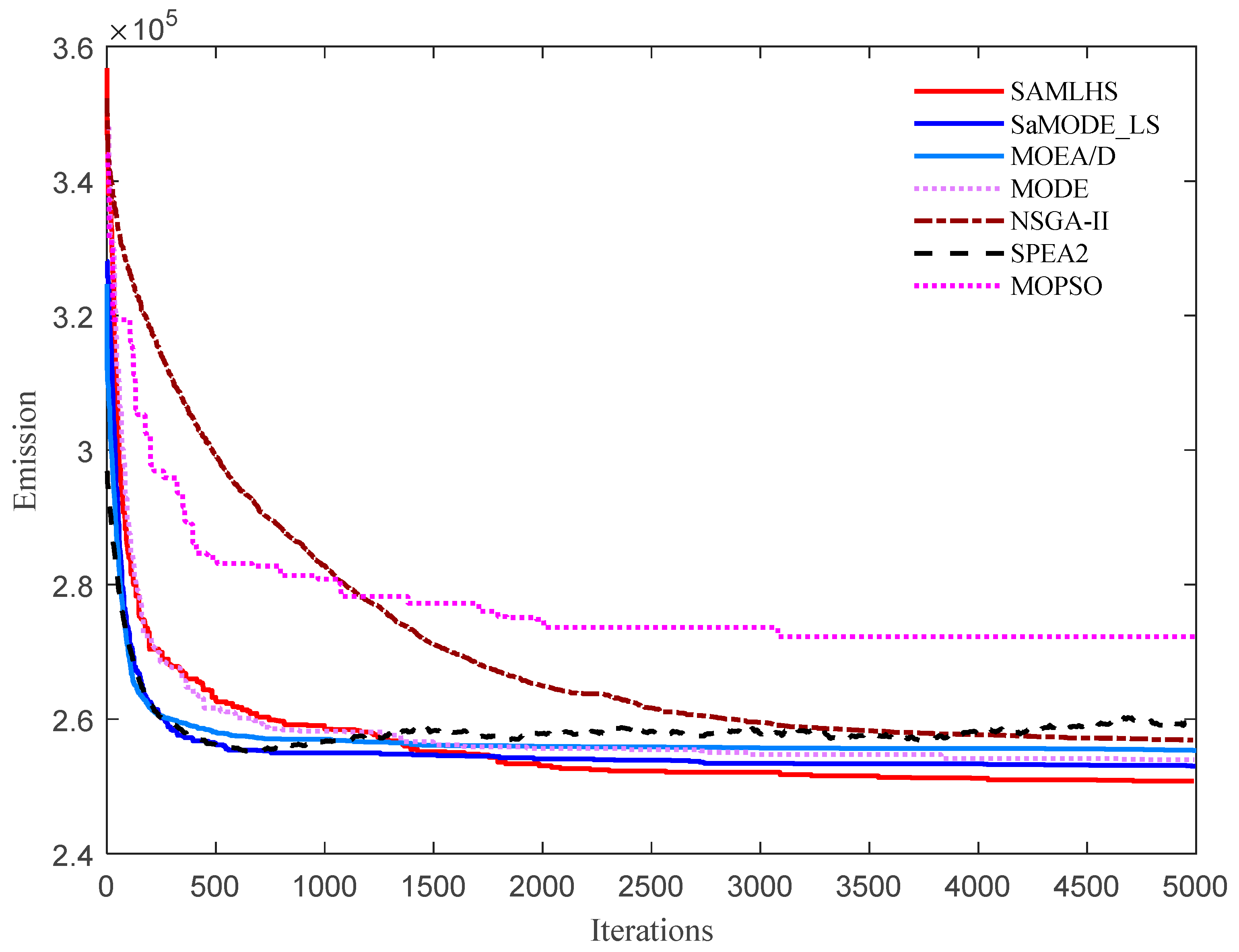
5.1. Verifying the Effectiveness of the Proposed SAMLHS Algorithm
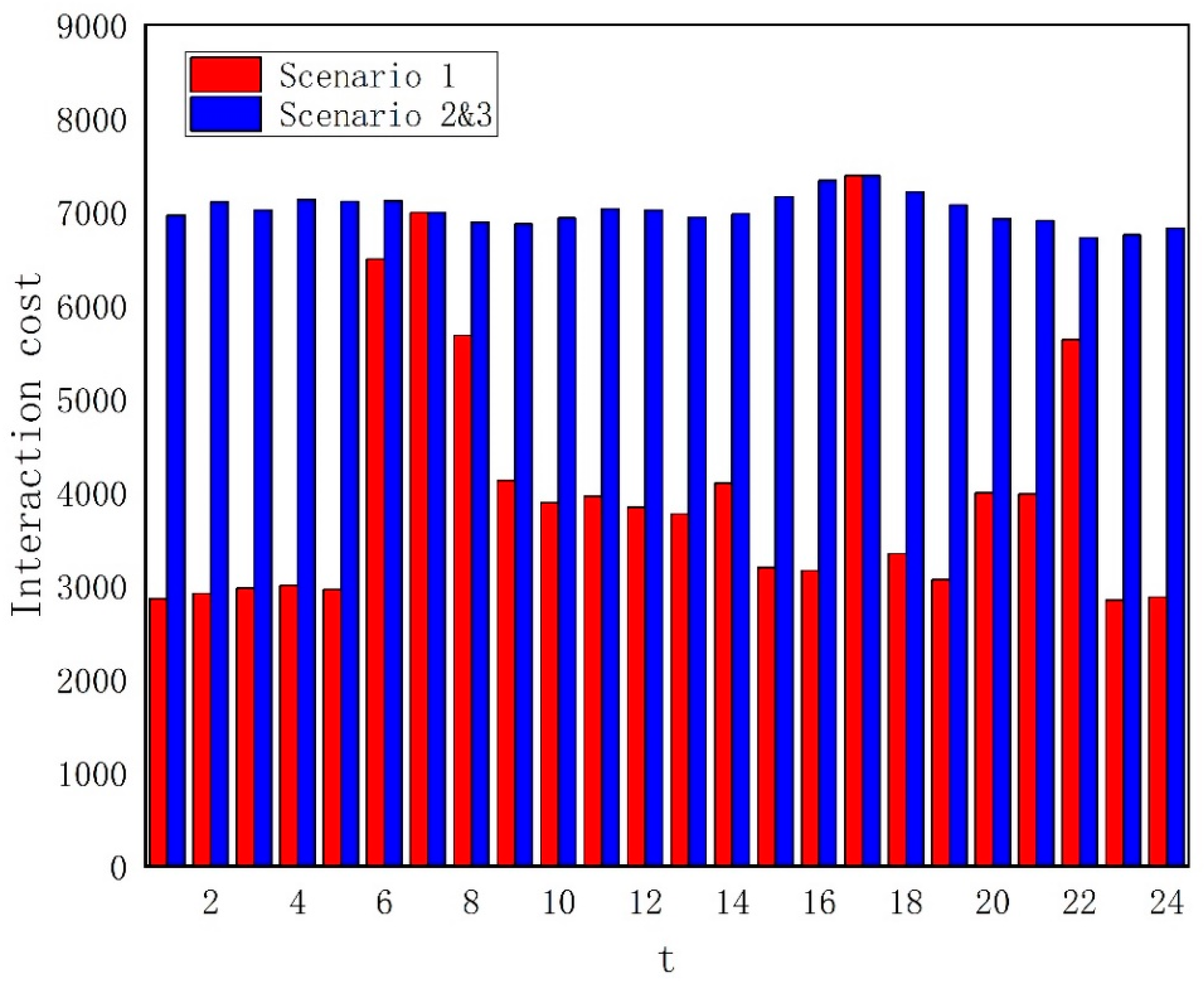
In this subsection, 50,000 EVs and 100 wind turbines were selected in the DEED IWEv model. To verify the performance of the proposed SAMLHS algorithm, it was compared to the six state-of-the-art algorithms. All algorithms used the same constraint-handling method, introduced in Section 3.3. Each algorithm was run 30 times independently.
The obtained Pareto Frontiers (PFs) of all the algorithms are shown in Figure 1. Note that PF refers to a set of Pareto optimal solutions obtained by one algorithm in the objective space. The proposed SAMLHS yields a PF with good distribution and convergence. It locates at the bottom of all the PFs and has the widest spread, indicating its superiority compared with other algorithms. Moreover, the basic HSA gets an unsatisfactory PF that may have fallen into the local region. It also demonstrates the effectiveness of our proposed self-adaptive multiple-learning strategies.
The extreme solutions, including the best cost and best emission solutions, and the compromise solutions, obtained by all the algorithms are shown in Table 6. We can see that both the best cost and the best emission are obtained by the proposed SAMLHS algorithm as 2.4294 × 10 6 $ and 2.5076 × 10 5 lb , respectively. This means that the proposed algorithm can provide the best choice for the decision-maker in terms of both cost and emission. As for the best compromise solution, the best cost and best emission are obtained by SAMLHS and SaMODE_LS, respectively; compared with the SAMLHS algorithm, SaMODE_LS increases by 0.974% in terms of Fc, although F M decreases by 0.701%. On balance, our proposed SAMLHS algorithm shows better performance in reducing the total cost and emissions of the system.
The convergence process of cost and emissions for the seven algorithms are plotted in Figure 2 and Figure 3, respectively. It can be seen that in terms of cost, the proposed SAMLHS shows a significant advantage in the convergence performance compared with other algorithms. In terms of emissions, the SaMODE_LS shows a faster convergence speed than the SAMLHS; however, the solution for the final convergence of the SAMLHS is better than that of SaMODE_LS. By comprehensive comparison, the proposed SAMLHS algorithm shows a better convergence performance than the other algorithms. The reason for this may be that the elite-learning strategy speeds up the convergence of the SAMLHS.
Detailed information for the compromise solution obtained by the SAMLHS is shown in Table 7. It can be seen that the charging of EVs is mainly concentrated from 23:00 to 6:00, which are the low load intervals of the day. During the load peak periods, from 08:00 to 14:00 and from 20:00 to 22:00, EVs discharge. This indicates that the dynamic management for EV charging and discharging is realized in the D E E D I W E v model. The power balance constraints can be checked for each interval in Figure 4.

5.2. Verifying the Proposed D E E D I W E v Model

To further validate the proposed DEED IWEv model, the following three scenarios were proposed to make a comparison. In Scenario 1, our proposed DEED IWEv model was employed, where EVs interact with wind power and both participate in the whole system. Scenario 2 was that EVs and wind power are involved in the entire system independently—the charging and discharging behavior of EVs no longer interact with wind power. The charging of EVs is provided by thermal power generators. Scenario 3 was that only wind power is involved in the whole system and EVs are no longer involved.
Table 8 shows the extreme solutions obtained for the three scenarios, including best cost and best emission. First, comparing Scenario 2 and Scenario 3, we find that both the best cost and best emission of Scenario 2 are lower than those in Scenario 3. This shows that a certain number of EVs involved in the system can reduce the total costs and emissions. Next, comparing Scenario 1 and Scenario 2, we find that the F C and F M of Scenario 1 are reduced by 5.467% and 0.740%, respectively, compared with those of Scenario 2; this indicates that the interaction between EVs and wind power can reduce the cost and emission of the system.
Table 9 shows the best compromise solutions obtained for the three scenarios. Comparing Scenario 2 and Scenario 3, the same conclusion can be drawn as in Table 7. Compared with Scenario 1, Scenario 2 shows a decrease of 0.448% in F M but an increase of 5.667% and 3.160% in F C and F P , respectively. Figure 5 shows the cost of interaction between EVs and wind power at different periods. As analyzed in Section 2.3, although EVs and wind power do not interact in Scenario 2 and Scenario 3, the curtailment and reserve costs for wind power are considered the same as the interaction cost. It can be seen that the interaction cost for Scenario 1 is always the smallest at different dispatch intervals.

5.3. Different Confidence Levels

In this subsection, the impact of different confidence levels on the DEED IWEv model is investigated. Note that the values of η   1 and η   2 are the same. Table 10 shows the extreme solutions obtained at different confidence levels. We found that the results deteriorate when the confidence level increases from 0.8 to 0.85, and improve when the level increases from 0.85 to 0.95. The worst results are obtained at a confidence level of 0.85, and the best results are at a confidence level of 0.95.
Table 11 shows the best compromise solutions obtained at different confidence levels. The best cost and emission values, 2.4620 × 10 6   $ and 2.6105 × 10 5   lb , were obtained at a confidence level of 0.9, but the minimum fuel cost was taken at a confidence level of 0.95. This suggests that the system may consume less fossil fuel when the confidence level increases. By comprehensive comparison, the best choice of confidence level is 0.95. Figure 6 shows the cost of the interaction between EVs and wind power at different confidence levels. It can be seen that the interaction costs obtained at different confidence levels show little difference.

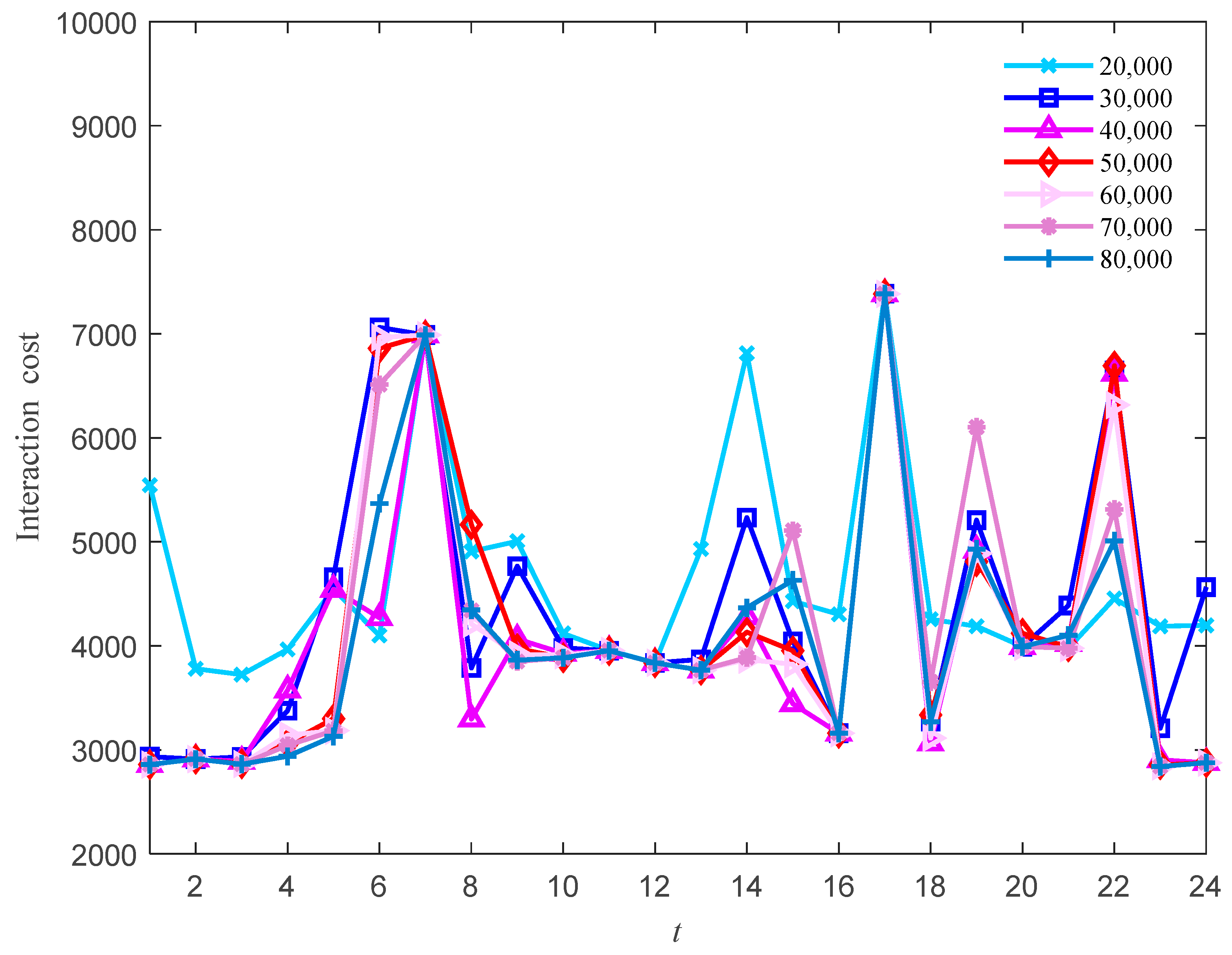
5.4. Different Scales of EVs and Wind Power

In this subsection, the impact of different scales of EVs and wind power on the DEED IWEv model is investigated.
Different scales of EVs: Table 12 shows the extreme solutions obtained with different scales of EVs. In the process of increasing the number of EVs, the best cost tends to increase and then decrease, taking the best value of 2.4294 × 10 6 $ at 50,000 vehicles; the best emission shows the same trend, taking the best value of 2.5040 × 10 5 lb at 60,000 vehicles.
Table 13 shows the best compromise solution obtained with different scales of EVs. At 50,000 EVs, the total cost and emission are taken to a minimum of 2.4632 × 10 6   $ and 2.6122 × 10 5   lb , which is a significant reduction compared with the other cases. In summary, the number of EVs involved in the system indeed affects the system performance. When the number of EVs is too small, it cannot bring much benefit to the system, and when the number of EVs is too large, it will be a burden on the system. Therefore, setting 50,000 electric vehicles is the best choice in our proposed DEED IWEv model. Figure 7 shows the cost of the interaction between EVs and wind power with different numbers of EVs.
Different wind power: Table 14 shows the extreme solutions obtained with different wind powers. The best cost 2.4294 × 10 6   $ is obtained when the P r a t e is 200 MW. With the increase in wind power, the optimal emission is reduced. This indicates that as wind power increases, the power generated by conventional thermal units can be reduced, but the cost of wind power generation also increases, resulting in a consistent increase in the total cost.
Table 15 shows the best compromise solutions obtained with different wind powers. The best cost is also reached when the Prate is 200 MW, the same as in Table 13. The best emission and fuel costs are 1.8129 × 10 5 lb and 2.0575 × 10 6 $ , respectively, when the Prate is 800 MW, while the cost of wind power generation reaches a maximum of 348,080. Therefore, when cost is the major consideration of the system, setting the wind power to 200 seems more suitable. Figure 8 shows the cost of the interaction between EVs and wind power. We can see that the interaction cost increases with the increase in wind power.

6. Conclusions

In this paper, a model based on the interaction between EVs and wind power ( IWEv ) is proposed, and further, a multi-objective DEED IWEv model is proposed based on the considerations of total cost and emission. Moreover, a novel multi-objective self-adaptive multiple-learning harmony-search algorithm is proposed to solve the DEED IWEv problem. In order to verify the effectiveness of the proposed algorithm and model, a 10-unit test system combining EVs and wind power is utilized. Results show that the proposed algorithm always shows a better performance compared with other advanced algorithms in terms of both total cost and emission. The proposed DEED IWEv model was validated by setting three different scenarios, and the results show that the proposed IWEv model performs better in terms of reducing cost and emission. In addition, the proposed model was tested under different confidence levels, numbers of EVs, and scales of wind power, and finally, the most suitable parameter configuration for the system is recommended. In our future work, other renewable energy sources will be considered for integration to the dispatching system.

Author Contributions

Conceptualization, L.Y., Z.Z., and B.Q. (Boyang Qu); methodology, L.Y., B.Q. (Boyang Qu), and Z.Z.; software, L.Y. and Z.Z.; validation, L.Y. and Z.Z.; formal analysis, B.Q. (Boyang Qu) and X.C.; data curation, X.K.; writing—original draft preparation, L.Y., X.C., and Z.Z.; writing—review and editing, B.Q. (Boyang Qu), X.C., and B.Q. (Baihao Qiao); supervision, J.H.; project administration, L.Y. and B.Q. (Boyang Qu). All authors have read and agreed to the published version of the manuscript.

Funding

This work was supported by the National Natural Science Foundation of China (Grant Nos. 62103456, 61976237), the Science and Technology Innovation Team of Colleges and Universities in Henan Province (Grant No. 22IRTSTHN015), the “Central Plains Thousand Talents Plan”-Top Talents in Central Plains (Grant No. ZYQR201810162), the Natural Science Foundation of Henan Province (Grant Nos. 212300410321, 202300410511), the Research Award Fund for Outstanding Young Teachers in Henan Provincial Institutions of Higher Education (Grant Nos. 2021GGJS111, 2020GGJS141), and the Fundamental Research Funds of Zhongyuan University of Technology (Grant No. K2020YY009).

Conflicts of Interest

The authors declare no conflict of interest.

References

  1. Yan, L.; Qu, B.; Zhu, Y.; Qiao, B.; Suganthan, P.N. Dynamic economic emission dispatch based on multi-objective pigeon-inspired optimization with double disturbance. Sci. China Inf. Sci. 2019, 62, 70210–70211. [Google Scholar] [CrossRef] [Green Version]
  2. Zhang, Y.; Liu, K.; Liao, X.; Qin, L.; An, X. Stochastic dynamic economic emission dispatch with unit commitment problem considering wind power integration. Int. Trans. Electr. Energy 2018, 28, e2472. [Google Scholar] [CrossRef]
  3. Chen, J.J.; Qi, B.X.; Peng, K.; Li, Y.; Zhao, Y.L. Conditional value-at-credibility for random fuzzy wind power in demand response integrated multi-period economic emission dispatch. Appl. Energy 2020, 261, 114337. [Google Scholar] [CrossRef]
  4. Liu, Z.; Li, L.; Liu, Y.; Liu, J.; Li, H.; Shen, Q. Dynamic economic emission dispatch considering renewable energy generation: A novel multi-objective optimization approach. Energy 2021, 235, 121407. [Google Scholar] [CrossRef]
  5. Liu, X.; Xu, W. Minimum Emission Dispatch Constrained by Stochastic Wind Power Availability and Cost. IEEE Trans. Power Syst. 2010, 25, 1705–1713. [Google Scholar]
  6. Zhang, Z.; Sun, Y.; Gao, D.W.; Lin, J.; Cheng, L. A Versatile Probability Distribution Model for Wind Power Forecast Errors and Its Application in Economic Dispatch. IEEE Trans. Power Syst. 2013, 28, 3114–3125. [Google Scholar] [CrossRef]
  7. Hu, F.; Hughes, K.J.; Ingham, D.B.; Ma, L.; Pourkashanian, M. Dynamic economic and emission dispatch model considering wind power under Energy Market Reform: A case study. Int. J. Electr. Power 2019, 110, 184–196. [Google Scholar] [CrossRef] [Green Version]
  8. Aghaei, J.; Niknam, T.; Azizipanah-Abarghooee, R.; Arroyo, J.M. Scenario-based dynamic economic emission dispatch considering load and wind power uncertainties. Int. J. Electr. Power 2013, 47, 351–367. [Google Scholar] [CrossRef]
  9. Jangir, P.; Jangir, N. A new Non-Dominated Sorting Grey Wolf Optimizer (NS-GWO) algorithm: Development and application to solve engineering designs and economic constrained emission dispatch problem with integration of wind power. Eng. Appl. Artif. Intel. 2018, 72, 449–467. [Google Scholar] [CrossRef]
  10. Chen, M.; Zeng, G.; Lu, K. Constrained multi-objective population extremal optimization based economic-emission dispatch incorporating renewable energy resources. Renew Energy 2019, 143, 277–294. [Google Scholar] [CrossRef]
  11. Hagh, M.T.; Kalajahi, S.M.S.; Ghorbani, N. Solution to economic emission dispatch problem including wind farms using Exchange Market Algorithm Method. Appl. Soft Comput. 2020, 88, 106044. [Google Scholar] [CrossRef]
  12. Jin, J.; Zhou, D.; Zhou, P.; Miao, Z. Environmental/economic power dispatch with wind power. Renew Energy 2014, 71, 234–242. [Google Scholar] [CrossRef]
  13. Zakariazadeh, A.; Jadid, S.; Siano, P. Multi-objective scheduling of electric vehicles in smart distribution system. Energ. Convers Manag. 2014, 79, 43–53. [Google Scholar] [CrossRef]
  14. Clement-Nyns, K.; Haesen, E.; Driesen, J. The Impact of Charging Plug-In Hybrid Electric Vehicles on a Residential Distribution Grid. IEEE Trans. Power Syst. 2010, 25, 371–380. [Google Scholar] [CrossRef] [Green Version]
  15. Wu, T.; Yang, Q.; Bao, Z.; Yan, W. Coordinated Energy Dispatching in Microgrid With Wind Power Generation and Plug-in Electric Vehicles. IEEE Trans. Smart Grid. 2013, 4, 1453–1463. [Google Scholar] [CrossRef]
  16. Gholami, A.; Ansari, J.; Jamei, M.; Kazemi, A. Environmental/economic dispatch incorporating renewable energy sources and plug-in vehicles. IET Gener. Transm. Distrib. 2014, 8, 2183–2198. [Google Scholar] [CrossRef]
  17. Zhao, Y.; Noori, M.; Tatari, O. Vehicle to Grid regulation services of electric delivery trucks: Economic and environmental benefit analysis. Appl. Energy 2016, 170, 161–175. [Google Scholar] [CrossRef]
  18. De Los Rios, A.; Goentzel, J.; Nordstrom, K.E.; Siegert, C.W. Economic Analysis of Vehicle-to-Grid (V2G)-Enabled Fleets Participating in the Regulation Service Market. In Proceedings of the 2012 IEEE PES Innovative Smart Grid Technologies (ISGT), Washington, DC, USA, 16–20 January 2012; pp. 1–8. [Google Scholar]
  19. Han, S.; Han, S. Economic Feasibility of V2G Frequency Regulation in Consideration of Battery Wear. Energies 2013, 6, 748–765. [Google Scholar] [CrossRef] [Green Version]
  20. Andersson, S.L.; Elofsson, A.K.; Galus, M.D.; Göransson, L.; Karlsson, S.; Johnsson, F.; Andersson, G. Plug-in hybrid electric vehicles as regulating power providers: Case studies of Sweden and Germany. Energy Policy 2010, 38, 2751–2762. [Google Scholar] [CrossRef]
  21. Qiao, B.; Liu, J. Dynamic Economic Dispatch with Electric Vehicles Considering Battery Wear Cost Using a Particle Swarm Optimization Algorithm. In Proceedings of the 2021 International Conference on Power System Technology (POWERCON), Haikou, China, 8–9 December 2021; pp. 807–813. [Google Scholar]
  22. Qiao, B.; Liu, J. Using Multi-Objective Particle Swarm Optimization to Solve Dynamic Economic Emission Dispatch Considering Wind Power and Electric Vehicles; Springer: Singapore, 2020; pp. 65–76. [Google Scholar]
  23. Qu, B.; Qiao, B.; Zhu, Y.; Liang, J.; Wang, L. Dynamic Power Dispatch Considering Electric Vehicles and Wind Power Using Decomposition Based Multi-Objective Evolutionary Algorithm. Energies 2017, 10, 1991. [Google Scholar] [CrossRef] [Green Version]
  24. Zhang, Y.; Le, J.; Liao, X.; Zheng, F.; Liu, K.; An, X. Multi-objective hydro-thermal-wind coordination scheduling integrated with large-scale electric vehicles using IMOPSO. Renew Energy 2018, 128, 91–107. [Google Scholar] [CrossRef]
  25. Zou, Y.; Zhao, J.; Ding, D.; Miao, F.; Sobhani, B. Solving dynamic economic and emission dispatch in power system integrated electric vehicle and wind turbine using multi-objective virus colony search algorithm. Sustain. Cities Soc. 2021, 67, 102722. [Google Scholar] [CrossRef]
  26. Lodewijks, G.; Cao, Y.; Zhao, N.; Zhang, H. Reducing CO2 emissions of an airport baggage handling transport system using a particle swarm optimization algorithm. IEEE Access 2021, 9, 121894–121905. [Google Scholar] [CrossRef]
  27. Shaukat, N.; Ahmad, A.; Mohsin, B.; Khan, R.; Khan, S.U.; Khan, S.U. Multiobjective Core Reloading Pattern Optimization of PARR-1 Using Modified Genetic Algorithm Coupled with Monte Carlo Methods. Sci. Technol. Nucl. Install. 2021, 2021, 1–13. [Google Scholar] [CrossRef]
  28. Basu, M. Particle Swarm Optimization Based Goal-Attainment Method for Dynamic Economic Emission Dispatch. Electr. Power Compon. Syst. 2006, 34, 1015–1025. [Google Scholar] [CrossRef]
  29. Neshat, M.; Nezhad, M.M.; Abbasnejad, E.; Mirjalili, S.; Groppi, D.; Heydari, A.; Tjernberg, L.B.; Astiaso Garcia, D.; Alexander, B.; Shi, Q.; et al. Wind turbine power output prediction using a new hybrid neuro-evolutionary method. Energy 2021, 229, 120617. [Google Scholar] [CrossRef]
  30. Bilal, B.; Adjallah, K.H.; Sava, A.; Yetilmezsoy, K.; Kıyan, E. Wind power conversion system model identification using adaptive neuro-fuzzy inference systems: A case study. Energy 2022, 239, 122089. [Google Scholar] [CrossRef]
  31. Duca, V.E.L.A.; Fonseca, T.C.O.; Cyrino Oliveira, F.L. Joint modelling wind speed and power via Bayesian Dynamical models. Energy 2022, 247, 123431. [Google Scholar] [CrossRef]
  32. Qiao, B.; Liu, J. Multi-objective dynamic economic emission dispatch based on electric vehicles and wind power integrated system using differential evolution algorithm. Renew Energy 2020, 154, 316–336. [Google Scholar] [CrossRef]
  33. Qiao, B.; Liu, J.; Hao, X. A multi-objective differential evolution algorithm and a constraint handling mechanism based on variables proportion for dynamic economic emission dispatch problems. Appl. Soft Comput. 2021, 108, 107419. [Google Scholar] [CrossRef]
  34. Li, Y.; Ni, Z.; Zhao, T.; Yu, M.; Liu, Y.; Wu, L.; Zhao, Y. Coordinated Scheduling for Improving Uncertain Wind Power Adsorption in Electric Vehicles—Wind Integrated Power Systems by Multiobjective Optimization Approach. IEEE Trans. Ind. Appl. 2020, 56, 2238–2250. [Google Scholar] [CrossRef]
  35. Khoa, T.H.; Vasant, P.M.; Singh, M.S.B.; Dieu, V.N. Swarm based mean-variance mapping optimization for convex and non-convex economic dispatch problems. Memet. Comput. 2017, 9, 91–108. [Google Scholar] [CrossRef]
  36. Ingram, G.; Zhang, T. Overview of Applications and Developments in the Harmony Search Algorithm; Springer: Berlin/Heidelberg, Germany, 2009; pp. 15–37. [Google Scholar]
  37. Society, F.C.S. Simulation; Simulation Councils, Inc.: San Diego, CA, USA, 1963. [Google Scholar]
  38. Deb, K.; Pratap, A.; Agarwal, S.; Meyarivan, T. A fast and elitist multiobjective genetic algorithm: NSGA-II. IEEE Trans. Evolut. Comput. 2002, 6, 182–197. [Google Scholar] [CrossRef] [Green Version]
  39. Zitzler, E.; Deb, K.; Thiele, L. Comparison of multiobjective evolutionary algorithms: Empirical results. Evol. Comput. 2000, 8, 173–195. [Google Scholar] [CrossRef] [Green Version]
  40. Yu, K.; Wang, X.; Wang, Z. Self-adaptive multi-objective teaching-learning-based optimization and its application in ethylene cracking furnace operation optimization. Chemometr. Intell. Lab. 2015, 146, 198–210. [Google Scholar] [CrossRef]
  41. Qu, B.Y.; Li, G.S.; Guo, Q.Q.; Yan, L.; Chai, X.Z.; Guo, Z.Q. A Niching Multi-objective Harmony Search Algorithm for Multimodal Multi-objective Problems. In Proceedings of the 2019 IEEE Congress on Evolutionary Computation (CEC), Wellington, New Zealand, 10–13 June 2019; pp. 1267–1274. [Google Scholar]
  42. Price, K.; Storn, R.M.; Lampinen, J.A. Differential Evolution—A Practical Approach to Global Optimization; Springer: Berlin, Germany, 2005. [Google Scholar]
  43. Eiben, A.E.; Hinterding, R.; Michalewicz, Z. Parameter control in evolutionary algorithms. IEEE T Evolut. Comput. 1999, 3, 124–141. [Google Scholar] [CrossRef] [Green Version]
  44. Zhang, Q.; Li, H. MOEA/D: A Multiobjective Evolutionary Algorithm Based on Decomposition. IEEE Trans. Evolut. Comput. 2007, 11, 712–731. [Google Scholar] [CrossRef]
  45. Huang, V.L.; Suganthan, P.N.; Liang, J.J. Comprehensive learning particle swarm optimizer for solving multiobjective optimization problems. Int. J. Intell. Syst. 2006, 21, 209–226. [Google Scholar] [CrossRef]
  46. Basu, M. Fuel constrained economic emission dispatch using nondominated sorting genetic algorithm-II. Energy 2014, 78, 649–664. [Google Scholar] [CrossRef]
  47. Abido, M.A. Multiobjective evolutionary algorithms for electric power dispatch problem. IEEE Trans. Evolut. Comput. 2006, 10, 315–329. [Google Scholar] [CrossRef]
Figure 1. The PFs obtained by different algorithms.
Energies 15 04942 g001
Figure 2. The convergence of cost for different algorithms.
Energies 15 04942 g002
Figure 3. The convergence of emission for different algorithms.
Energies 15 04942 g003
Figure 4. Constraints checking for the best compromise solution.
Energies 15 04942 g004
Figure 5. Interaction cost between EVs and wind power for different scenarios.
Energies 15 04942 g005
Figure 6. Interaction cost obtained at different confidence levels.
Energies 15 04942 g006
Figure 7. Interaction cost obtained with different scales of EVs.
Energies 15 04942 g007
Figure 8. Interaction cost obtained with different wind powers.
Energies 15 04942 g008
Table 1. System parameters and their descriptions.
ParametersDescription
v t wind speed at time t
k t , c t shape and scale parameters
μ t , σ t mean value and the standard deviation of wind speed
P r a t e rated power of the wind turbines
v r a t e , v i n ,   v o u t rated wind speed, the cut-in wind speed and cut-out wind speed
P e . i , N e rated power of the i th EV, number of EVs
P w . c u r , P w . n c u r wind power curtailment and no curtailment of I W E v system
P w a . j . t actual wind power from the j th wind turbine at time t
P w d i s . j . t dispatch power of the j th wind turbine at time t
T , N dispatching period, the number of units
α i , β i , γ i , ζ i , φ   i cost coefficients of the i th unit
P i . t the active power of the i th unit at time t
D j . t direct cost coefficient of the j th wind turbine
N w number of wind turbines
C c w j . t , C r w j . t cost coefficient for wind power curtailment and reserve
F i n t cost of interaction between wind power and EVs.
a i , b i , c i , d i ,   e i emission coefficients of the i th unit
P D . t , P L . t load demand of the system at time t , system loss at time t
B i j , B i 0 ,   B 00 coefficients of the B-coefficient method
E c o n . t amount of power consumed during the driving of EV
E , L power consumption per unit time of EVs driving, driving distance.
C   and   D , t charging and discharging efficiency, dispatch interval.
P R c h ,     P R D c h charging and discharging rate power
U R t and D R t Increase and decrease the rate of the thermal power unit at time t
ω u and ω d spinning reserve coefficients of the wind power
ϑ u and ϑ d reserve coefficients of EVs
η 1 and η 2 two pre-specified confidence levels
S R . t u spinning reserve demand at time t
NPpopulation size
iterationthe number of iterations
FEsfunction evaluations
r penalty coefficient
ε threshold value
K maximum adjustment
P R c h , P R D c h rate power charging and discharging
SOCremaining capacity of electric vehicle batteries
Table 2. The description of EV charging and discharging states.
StateDescription
charging x < 0 , sign ( x ) = −1 and P c h . t < 0, the dispatch system needs to provide power for the EVs.
discharging x > 0 , sign ( x ) = 1 and P D c h . t > 0, the EVs can feedback power to the dispatch system.
No charging/discharging x = 0 , EVs do not participate in the power system dispatch.
Table 3. Algorithm parameters.
AlgorithmDescription
SAMLHS [41] H M C R m a x and H M C R m i n were set to 0.95 and 0.06, P A R m a x and P A R m i n were set to 0.95 and 0.35.
SaMODE_LS [32]Ls was set to 0.1, F m i n and F m a x were set to 0.3 and 0.9,   C R m i n and C R m a x were set to 0.1 and 0.9, and the DE/rand/1 operation was employed.
MODE [42,43] F and C R were set to 0.5 and 0.5, and the DE/rand/1 operation was employed.
MOEA/D [44] F and C R were set to 0.6 and 0.9, respectively. Both the distribution indexes and neighborhood size were set to 20. The mutation rate was set to 1/d.
MOPSO [45]the personal and global learning coefficients were set to 2.05. The inertia weight coefficient was set to 0.729.
NSGA-II [46]the crossover and mutation probabilities were set to 0.9 and 0.2. The distribution indices for crossover and mutation operators were η c   = 20 and η m   = 20, respectively.
SPEA2 [47]the crossover and mutation probabilities were set to 0.7 and 0.3, respectively, and the archive size was set to 100.
Table 4. Comparison of the IGD measure between SAMLHS and other MOEAs, mean (Std).
ProblemsSAMLHSSaMODE_LSMOEA/DMODENSGA-IISPEA2MOPSO
ZDT1 4.799 × 10 3
( 5.54 × 10 8 )
6.108 × 10 3
( 9.59 × 10 8 )+
5.265 × 10 3
( 1.86 × 10 7 )+
1.442 × 10 2
( 3.79 × 10 6 )+
4.732 × 10 3
( 1.53 × 10 4 )=
3.962 × 10 3
  ( 5.83 × 10 5 )−
1.819 × 10 2
  ( 3.572 × 10 5 )+
ZDT2 4.713 × 10 3
( 5.24 × 10 8 )
5.734 × 10 3
( 4.84 × 10 8 )+
4.409 × 10 3
  ( 3.90 × 10 8 )−
2.021 × 10 2
( 1.16 × 10 5 )+
4.894 × 10 3
  ( 1.72 × 10 4 )+
3.942 × 10 3
  ( 5.44 × 10 5 )−
6.968 × 10 1
  ( 9.07 × 10 3 )+
ZDT3 5.109 × 10 3
( 5.24 × 10 8 )
5.818 × 10 3
( 5.44 × 10 8 )+
1.022 × 10 2
  ( 1.10 × 10 8 )+
2.136 × 10 2
( 1.42 × 10 5 )+
6.415 × 10 3
  ( 5.33 × 10 3 )+
6.164 × 10 3
  ( 5.52 × 10 3 )+
5.498 × 10 2
  ( 5.36 × 10 4 )+
ZDT4 4.661 × 10 3
( 7.84 × 10 8 )
4.743 × 10 3
( 7.20 × 10 8 )=
3.865 × 10 3
  ( 1.86 × 10 10 )−
4.513 × 10 3
( 5.173 × 10 8 )−
5.938 × 10 3
  ( 1.27 × 10 3 )+
5.194 × 10 3
  ( 1.50 × 10 3 )=
2.998 × 10 1
  ( 1.62 × 10 1 )+
ZDT6 3.259 × 10 3
( 1.71 × 10 7 )
3.300 × 10 3
( 2.81 × 10 7 )=
2.059 × 10 3
  ( 8.37 × 10 11 )−
3.398 × 10 3
( 3.42 × 10 7 )=
3.736 × 10 3
  ( 1.35 × 10 4 )+
3.145 × 10 3
  ( 4.84 × 10 5 )=
3.392 × 10 3
  ( 2.38 × 10 7 )=
Sum-up +\=\−3\2\02\0\33\1\14\1\01\2\24\1\0
Table 5. System and EV parameter settings.
ParametersValueParametersValue
NP100Battery capacity21.6 kWh
iteration5000 E 0.139 kWh/km
FEs500,000 L 43 km
D j . t 50Travel time 07 : 00 08 : 00   and   17 : 00 18 : 00 ,   other   time   participate   in   the   I W E v system
C c w j . t ,   C r w j . t 75
η 1 ,   η 2 0.95Initial SOC100%
T24 hMinimum SOC20% of the battery capacity
C ,   D 0.85 P R c h ,   P R D c h 20% of the battery capacity
ϑ u ,   ϑ d 0.3 K 10
r 100 ε 10 6
Table 6. The solutions for different algorithms ( F C ( × 10 6 $ ) ) and ( F M ( × 10 5 lb ) ).
AlgorithmsSAMLHSSaMODE_LSMODEMOEA/D
F C F M F C F M F C F M F C F M
Best cost2.42942.82322.44952.74812.44002.80922.54922.7102
Best emission2.55232.50762.54522.52982.54832.53972.63472.5535
Best compromise2.46322.61222.48722.59392.47062.62992.57872.6048
AlgorithmsNSGA-IISPEA2MOPSO
F C F M F C F M F C F M
Best cost2.52722.60502.55282.63502.54612.7863
Best emission2.53542.56862.56612.59552.59882.7486
Best compromise2.53192.57432.55772.61552.57472.7793
Table 7. The best compromise solution obtained by SAMLHS.
t P 1 P 2 P 3 P 4 P 5 P 6 P 7 P 8 P 9 P 10 V 2 G P w d P L P D
1152.00137.07113.99136.89174.91143.3099.93103.5658.6033.16−162.9094.2848.801036
2155.49138.16121.96117.50208.19158.73120.25119.0278.4547.56−199.6095.9251.641110
3156.99140.79143.91143.51212.62150.45126.50118.1679.1051.55−105.58101.2461.241258
4173.87170.04179.96191.12225.68159.53129.05118.8079.3553.86−109.59101.0966.751406
5175.63198.57208.89191.49236.87158.49129.16118.6979.3053.80−101.2598.5968.231480
6169.01198.66250.58202.35243.00159.95130.00120.0079.9954.92−7.8594.8967.501628
7176.62201.13255.06261.45242.82159.68130.00119.7879.8154.850.0089.6768.871702
8189.59250.27250.70243.97242.70159.65129.87119.5479.2954.7437.8078.6660.781776
9240.10285.23270.18281.41242.60159.56129.53119.5779.7054.6951.0471.5561.161924
10253.66291.01313.35298.32242.93159.78129.59119.7979.7654.8672.8356.0149.892022
11263.62299.20311.10300.00243.00160.00130.00120.0080.0055.00138.0341.3935.342106
12250.77289.02329.82299.23242.82159.64129.48119.7379.5354.50162.7459.4749.752127
13259.70296.08330.73299.60242.57159.68129.68119.6879.6254.6892.2468.2760.532072
14236.42270.45274.26291.28242.73159.67129.71119.7079.6354.6848.7577.9561.231924
15256.29278.79259.94278.40242.81159.78129.23119.5279.9254.78−100.8876.3758.951776
16183.88221.07246.82258.48242.59159.77129.55119.4479.8254.76−171.4473.0643.801554
17156.59158.51172.34212.10202.48154.91127.73116.7377.7354.930.0080.8634.911480
18175.44237.40244.04250.07242.48159.71129.67119.5279.5754.47−90.0456.6530.981628
19240.62288.58258.79276.21242.80159.96129.58119.9679.6554.55−86.0134.4023.091776
20216.42283.88281.15299.31242.52159.81129.40119.9679.5354.4497.0536.2927.761972
21231.34257.17280.87277.88242.33159.47129.61119.7379.5754.6580.9040.7330.251924
22167.04196.41217.49231.88236.83159.53129.80119.6979.9854.7513.7858.6937.881628
23155.70145.74166.33198.91227.53158.15128.45118.2078.2649.74−126.3773.0441.681332
24161.55151.87132.79171.62201.94145.86126.27114.7177.5053.91−190.6581.3444.701184
Table 8. The extreme solutions of different scenarios.
ScenariosExtreme Solutions
F C   ( $ ) F M   ( l b )
1Best cost 2.4294 × 10 6 2.8232 × 10 5
Best emission 2.5523 × 10 6   2.5076 × 10 5
2Best cost 2.5699 × 10 6 2.7535 × 10 5
Best emission 2.6762 × 10 6 2.5263 × 10 5
3Best cost 2.5853 × 10 6 2.7668 × 10 5
Best emission 2.6731 × 10 6 2.5618 × 10 5
Table 9. The best compromise solutions for different scenarios.
ScenariosBest Compromise Solutions
F C   ( $ ) F M   ( l b ) F W   ( $ ) F i n t   ( $ ) F P   ( $ )
1 2.4632 × 10 6 2.6122 × 10 5 87,019100,718.432 2.2755 × 10 6
2 2.6028 × 10 6 2.6005 × 10 5 87,019168,338.7 2.3474 × 10 6
3 2.6172 × 10 6 2.6355 × 10 5 87,019168,338.7 2.3618 × 10 6
Table 10. The extreme solutions obtained at different confidence levels.
η   1 ,   η   2 Extreme Solutions
F C   ( $ ) F M   ( l b )
0.8Best cost 2.4328 × 10 6 2.7925 × 10 5
Best emission 2.5342 × 10 6 2.5190 × 10 5
0.85Best cost 2.4351 × 10 6 2.7953 × 10 5
Best emission 2.5388 × 10 6 2.5306 × 10 5
0.9Best cost 2.4300 × 10 6 2.7832 × 10 5
Best emission 2.5332 × 10 6 2.5123 × 10 5
0.95Best cost 2.4294 × 10 6 2.8232 × 10 5
Best emission 2.5523 × 10 6 2.5076 × 10 5
Table 11. The best compromise solutions obtained at different confidence levels.
η   1 ,   η   2 Best Compromise Solutions
F C   ( $ ) F M   ( lb ) F W   ( $ ) F i n t   ( $ ) F P   ( $ )
0.8 2.4722 × 10 6 2.5909 × 10 5 87019103,983.54 2.2812 × 10 6
0.85 2.4634 × 10 6 2.6219 × 10 5 87019100,438.48 2.2759 × 10 6
0.9 2.4620 × 10 6 2.6105 × 10 5 8701998,723.295 2.2763 × 10 6
0.95 2.4632 × 10 6 2.6122 × 10 5 87019100,718.43 2.2755 × 10 6
Table 12. The extreme solutions obtained with different scales of EVs.
EVsExtreme Solutions
F C   ( $ ) F M   ( l b )
20,000Best cost 2.5563 × 10 6 2.6746 × 10 5
Best emission 2.6169 × 10 6 2.5614 × 10 5
30,000Best cost 2.5212 × 10 6 2.7496 × 10 5
Best emission 2.6185 × 10 6 2.5459 × 10 5
40,000Best cost 2.5132 × 10 6 2.7668 × 10 5
Best emission 2.6149 × 10 6 2.5390 × 10 5
50,000Best cost 2.4294 × 10 6 2.8232 × 10 5
Best emission 2.5523 × 10 6 2.5076 × 10 5
60,000Best cost 2.5049 × 10 6 2.8540 × 10 5
Best emission 2.6412 × 10 6 2.5040 × 10 5
70,000Best cost 2.5252 × 10 6 2.6943 × 10 5
Best emission 2.6284 × 10 6 2.5061 × 10 5
80,000Best cost 2.5260 × 10 6 2.6923 × 10 5
Best emission 2.6375 × 10 6 2.5125 × 10 5
Table 13. The best compromise solutions obtained with different scales of EVs.
EVsBest Compromise Solutions
F C ( $ ) F M ( l b ) F W ( $ ) F i n t ( $ ) F P ( $ )
20,000 2.5817 × 10 6 2.6001 × 10 5 87,019111,574.49 2.3831 × 10 6
30,000 2.5685 × 10 6 2.5927 × 10 5 87,019106,148.157 2.3753 × 10 6
40,000 2.5416 × 10 6 2.6314 × 10 5 87,01997,532.175 2.3570 × 10 6
50,000 2.4632 × 10 6 2.6122 × 10 5 87,019100,718.432 2.2755 × 10 6
60,000 2.5438 × 10 6 2.6165 × 10 5 87,01998,733.36 2.3580 × 10 6
70,000 2.5697 × 10 6 2.5684 × 10 5 87,019100,274.5 2.3824 × 10 6
80,000 2.5666 × 10 6 2.5774 × 10 5 87,01997,256.729 2.3823 × 10 6
Table 14. The extreme solutions obtained with different wind power.
P r a t e ( M W ) Extreme Solutions
F C   ( $ ) F M   ( l b )
100Best cost 2.4802 × 10 6 2.9052 × 10 5
Best emission 2.5784 × 10 6 2.6832 × 10 5
200Best cost 2.4294 × 10 6 2.8232 × 10 5
Best emission 2.5523 × 10 6 2.5076 × 10 5
300Best cost 2.5516 × 10 6 2.6388 × 10 5
Best emission 2.6603 × 10 6 2.3838 × 10 5
400Best cost 2.5999 × 10 6 2.5364 × 10 5
Best emission 2.7383 × 10 6 2.2351 × 10 5
500Best cost 2.6630 × 10 6 2.4201 × 10 5
Best emission 2.7676 × 10 6 2.1114 × 10 5
600Best cost 2.7260 × 10 6 2.3269 × 10 5
Best emission 2.8346 × 10 6 1.9728 × 10 5
700Best cost 2.8011 × 10 6 2.1340 × 10 5
Best emission 2.9107 × 10 6 1.8597 × 10 5
800Best cost 2.8346 × 10 6 1.9728 × 10 5
Best emission 2.8346 × 10 6 1.9728 × 10 5
Table 15. The best compromise solutions obtained with different wind powers.
P r a t e     Best Compromise Solutions
F C   ( $ ) F M   ( l b ) F W   ( $ ) F i n t   ( $ ) F P   ( $ )
100 2.5184 × 10 6 2.7573 × 10 5 43,51048,898.751 2.4260 × 10 6
200 2.4632 × 10 6 2.6122 × 10 5 87,019100,718.432 2.2755 × 10 6
300 2.5870 × 10 6 2.4761 × 10 5 130,530158,878.096 2.2976 × 10 6
400 2.6429 × 10 6 2.3333 × 10 5 174,040222,744.63 2.2461 × 10 6
500 2.6950 × 10 6 2.2264 × 10 5 217,550296,158.08 2.1813 × 10 6
600 2.7581 × 10 6 2.0960 × 10 5 261,060378,812.1 2.1182 × 10 6
700 2.8414 × 10 6 1.9513 × 10 5 304,570456,864.1 2.0800 × 10 6
800 2.9259 × 10 6 1.8129 × 10 5 348,080547,279.6 2.0575 × 10 6
Publisher’s Note: MDPI stays neutral with regard to jurisdictional claims in published maps and institutional affiliations.

