
Modeling Results for the Real Horizontal Heavy-Oil-Production Well of Mechanical Solids

1
Gubkin Russian State University of Oil and Gas (National Research University), Leninskiy Prospect, 65, 119991 Moscow, Russia
2
Oil and Gas Faculty, Saint Petersburg Mining University, 199106 St. Petersburg, Russia
*
Author to whom correspondence should be addressed.
Energies 2022, 15(14), 5182; https://0-doi-org.brum.beds.ac.uk/10.3390/en15145182
Submission received: 14 June 2022
/
Revised: 2 July 2022
/
Accepted: 11 July 2022
/
Published: 17 July 2022
(This article belongs to the Special Issue Advances in Techniques of Construction, Development and Operation of Oil and Gas Wells)
Abstract
:Recently, more and more new oil fields entering commercial production are complicated by the content of high-viscosity products, which are located at relatively shallow depths. For the rational development of such fields, a network of horizontal wells is used. A special feature of these objects is a weakly cemented reservoir, which leads to significant sand occurrence during well operation. At the same time, the removal of mechanical impurities cannot be avoided even when using complex measures, including the use of various filters. There are quite a few methods describing the behavior of mechanical impurities in gas–liquid flows. The purpose of the work was to analyze the removal of mechanical impurity particles from horizontal wells with high-viscosity oil. A model of a typical well in the OLGA software was created, and data on the types of particle removal were obtained. As a result of calculations, the quality of removal for different diameters of mechanical impurities was determined, and the dependence of the critical diameter on the well flow rate was constructed.
1. Introduction
One of the potentials of the increased oil and gas production in the Russian Federation and the Western Siberian Province, in particular, is exploration and development of deposits composed of poorly cemented reservoirs, associated with the Upper Aptian-Cenomanian deposits. The Upper Aptian-Cenomanian reservoirs are concentrated under regionally consistent clay cover of Turonian age, and are associated with thick strata of alternating sandy–silty and siltstone–shaly rocks. The type of the deposit is massive, with underlying bottom water, while the reservoir type is predominantly pore, the lithological and reservoir properties of which are sufficiently studied [1,2,3]. Sandstone of Cenomanian deposits is represented by loose, poorly cemented rocks, therefore during drilling and testing, they are characterized by their destruction, wall collapse, formation of cavities, and sand mobilization into the wellbore [4,5,6].
Studies conducted in Russia and abroad demonstrate that during well development, testing, and operation, the solid particles drilled out of the bed are recovered due to destruction of natural cementing material therein. A non-cemented bed is considered to be a formation not containing a sufficient amount of natural cementing material in order to retain the composing rock of minerals in mutual contact during oil or gas inflow to the well [7,8].
Uncemented beds are found in almost all the main oil producing regions of the world. Problems of the formation of sand plugs in such fields often occur during construction of offshore wells and wells with pay beds represented by young formations. In this respect, most famous both on land and at sea are the Northern coast of the Gulf of Mexico; the Los Angeles Basin, California (Wilmington field); as well as areas of bituminous sands in Canada, Indonesia, Nigeria, Venezuela, and Trinidad and Tobago. Significant difficulties with sand are also observed at the Maracaibo Lake, the Norwegian shelf and other areas of the North Sea; the PRC shelf; the western coasts of Africa; and the central part of Russia. Similar deposits in Western Siberia were first opened at the Russkoye oil field at the end of 1960s and in the early 1970s [9,10].
At a number of new facilities in similar Russian deposits in Western Siberia, production is complicated by high viscosity of produced hydrocarbons. Therefore, the main part of the well stock is horizontal wells, where multi-stage hydraulic fracturing is carried out at the stage of completion. Taken together, these factors lead to the fact that mechanical impurities cannot be avoided even with utilization of integrated measures, such as strengthening of the near-wellbore formation zone with binding compositions with various types of completion, as well as application of sand screens [11,12].
Rock particles recovered from the formation block the bottomhole, accumulating in the horizontal section of the wellbore. This causes well shutdown and liner cleaning operations, resulting in significant downtime and losses in production [13,14].
The main method for limiting sand production is establishing optimum technological parameters of the well. This regime, on the one hand, must ensure a high oil production rate, and on the other hand, minimize accumulation of particles at the bottom hole to reduce the frequency of well interventions, which will have positive impact on field development indicators.
The purpose of this work was to analyze the withdrawal of mechanical impurities from horizontal wells producing high-viscosity oil. This will allow prediction of the process of accumulation of mechanical particles in the wellbore of the producer well, depending on the mode parameters. The study was carried out for the active oil field in the Yamal-Nenets Autonomous Region, which is at a stage of intensive development (conditionally named the «Training» field).
The goal was achieved through:
- Selection of an adequate analytical model for calculations.
- Creation of a model well of the «Training» field in the OLGA software.
- Calculations of the removal of particles at various well flow rates.
- Systematization of research results.
Much experimental work has been done on the hydraulic movement of fluids containing mechanical impurities, including by N.S. Blatch [15], which was later continued by R. Durand and E. Condolios [16,17], D.M. Newitt et al. [18], G.A. Hughmark [19], D.G. Thomas [20], Y. Yang et al. [21], and others. However, in most works, water was used as the carrier liquid. Determination of the influence of fluid viscosity on the nature of the transport of sand particles in horizontal pipes can be observed in the works of C.A. Shook et al. [22], G.A. Wani [23], R.G. Gillies et al. [24], and E. Zorgani et al. [25]. These studies were carried out on various media: ethylene glycol, kerosene, mineral oils, etc.
Worldwide, there are more than 60 models [26] describing the behavior of particles in the flow. The high number of works is attributable to the fact that the task of solids transfer and deposition is extremely complex and multifaceted. To correctly describe sand behavior, the following data should be taken into account: fluid velocity, tubing diameter (or borehole), gas velocity, fluid viscosity, geometry of particles and their concentration in the flow, particle density, and angle of casing (or borehole) inclination [27]. Unfortunately, in many models, one or another parameter is neglected, which limits their application area.
For example, Oroskar and Turian proposed a model in 1980 [28] that was originally intended for a single-phase flow. The model was extended in 2011 by Hill [29] for the possibility of gas phase metering. The strength of the technique is its taking into account of the concentration of particles and flow turbulence. However, a large number of parameters make the model difficult to use. According to Oroskar and Turian [21], the critical velocity (Expression 1) is the minimum velocity required for continuous non-settlement of moving particles.
where —critical velocity, m/s; —reduced liquid velocity, m/s; —particle diameter, m; D—pipe diameter, m; —density of particle, kg/m3; —liquid density, kg/m3; Re—Reynolds number; C—concentration of particles, %; —density difference between particles and liquid; —kinetic viscosity, cP; and —proportion of flow turbulence.
Salama developed a model in 1998 to determine the critical velocity in a single-phase flow, and later extended his methodology to a multi-phase flow [30]. The model of a single-phase flow was obtained by simplifying the model by Oroskar and Turian (1980). The critical velocity in [30] was calculated using the iterative method until the left part of Formula (2) was equal to the right. Disadvantages of this model include the impossibility of recording the impact of the particles’ concentration on their deposition. According to Salama [30], the critical velocity is defined as the minimum velocity required to maintain the particle in a weighted state.
Danielson created a model [31] in 2007 to forecast particle deposition in a single-phase flow and then extended it to multi-phase flow. The model is simple, but does not consider the impact of particles concentration on the critical velocity. According to Danielson [24], the critical velocity (Formula (3)) is the velocity required to prevent the formation of a “lying” layer.
This job was performed using the Schlumberger simulator OLGA [32]. Developers of this software created their own model based on multi-year studies by describing the behavior of particles in pipelines and wells under different fluid flow regimes.
In [33], the issue of proppant recovery after hydraulic fracturing with a changing well productivity factor (both its increase and decrease) was considered. The calculations were performed using the OLGA unsteady flow simulator. As a result of the study, it was found that the main part of the sand removed from the reservoir settled in the toe of the well. This was due to the accumulation of fluid flow when moving from the toe to the heel of the horizontal wellbore.
The study in [34] was also performed using the OLGA software. It addressed the issues of sand accumulation in horizontal wells with different horizontal section profiles, which included 90-degree horizontal, toe-up, toe-down, and sump and hump trajectories. The 90-degree horizontal and sump and hump trajectories have been proven to be superior to toe-up and toe-down trajectories in terms of preventing sand accumulation. The authors also carried out a sensitivity analysis of the influence of various parameters of the gas–liquid flow and the particles themselves on sand settling. For example, with an increase in water cut, sand production improved, which was associated with the formation of emulsions of a higher viscosity than the viscosity of non-watered oil. With an increase in particle diameter, sand production deteriorated. The graphs clearly showed the degradation of the recovery quality as the particle diameter increased.
The work of R. Dabirian and team [35] showed the results of a comprehensive study of sand movement in a two-phase flow. The authors identified six modes of sand behavior during movement: fully dispersed solid flow, dilute solids at wall, concentrated solids at wall, moving dunes, stationary dunes, and stationary bed. The study was carried out for a wide range of particle diameters and their concentrations in the flow, as well as for different velocities of the gas–liquid mixture. This work was carried out on a specially built stand at the University of Tulsi. Air was used as the gas phase, a viscous medium was modeled by adding polyanionic cellulose to water, and glass beads played the role of mechanical impurities. Experimental results showed that large particles (large diameter) had higher critical settling rates compared to small particles (small diameter).
2. Materials and Methods
OLGA software [32] allows simulating the flow with solid impurities on any part of the well in time. The model solves the equations of particle mass conservation in two fields: particles weighed in liquid layers, and particles in the “pillow”. The “pillow” layer consists of two sub-layers: a static part (called the fixed “pillow”) and a mobile part (called the mobile “pillow” or load on “pillow”). The entrainment and settling rate of particles determines the size of the layer, while the porosity of the layer (available as user input) determines the amount of liquid trapped in the layer. It is assumed that the fluid does not flow through the fixed layer.
The particles are assumed to be dispersed in three phases (gas layer, oil layer, and water). The particle velocity is defined by drift velocity or slip, defined as the particle velocity relative to the carrier phase velocity. Only gravity-induced slip is taken into account, and therefore particles flowing horizontally will move at the speed of the carrier phase if settling is not taken into account. The vertical slip between particles and phase, Vsl, is calculated depending on the Reynolds number.
For laminar flow (Re < 3), empirical correlation for Vsl is as follows [32]:
where ds—diameter of particles (m), ρs—density of solid particles (kg/m3), ρf—phase density (oil, water, gas) (kg/m3), µf—phase viscosity (oil, water, gas) (kg/m3), and Vsl—slip rate between particles and phase (m/s).
The Reynolds number for particles is based on Vsl and the diameter of particles:
For the transition flow (3 < Re < 300), empirical correlation for Vsl is equal to:
For the fully developed turbulent flow (Re > 300), empirical correlation for Vsl is equal to:
The axial slip is set to Vsl multiplied by the cosine angle (θ) of the pipe with a gravity vector:
The rate of deposition shall be determined as follows:
where S—length of the layer–suspension interface in the cross section, A—pipe area, and —concentration of suspended particles on the “pillow” surface.
The loss rate is defined as:
where Cb is the concentration of particles in the “pillow”.
The authors of [36] compared the data obtained using the OLGA software and other known methods: Oroskar and Turian (1980), Salama (2000), and Danielson (2007). The calculated values were compared with the experimental ones by constructing cross-plots. According to the analysis of the results, it may be concluded that the OLGA software performed well on a single-phase flow, but tended to underestimate the ability of a two-phase mixture to carry particles in a suspended state (the critical velocity defined by the OLGA software is below the real critical velocity). It should be noted that none of the studied methods could show satisfactory results on a two-phase flow (for all methods, individual points had an error of about 40%).
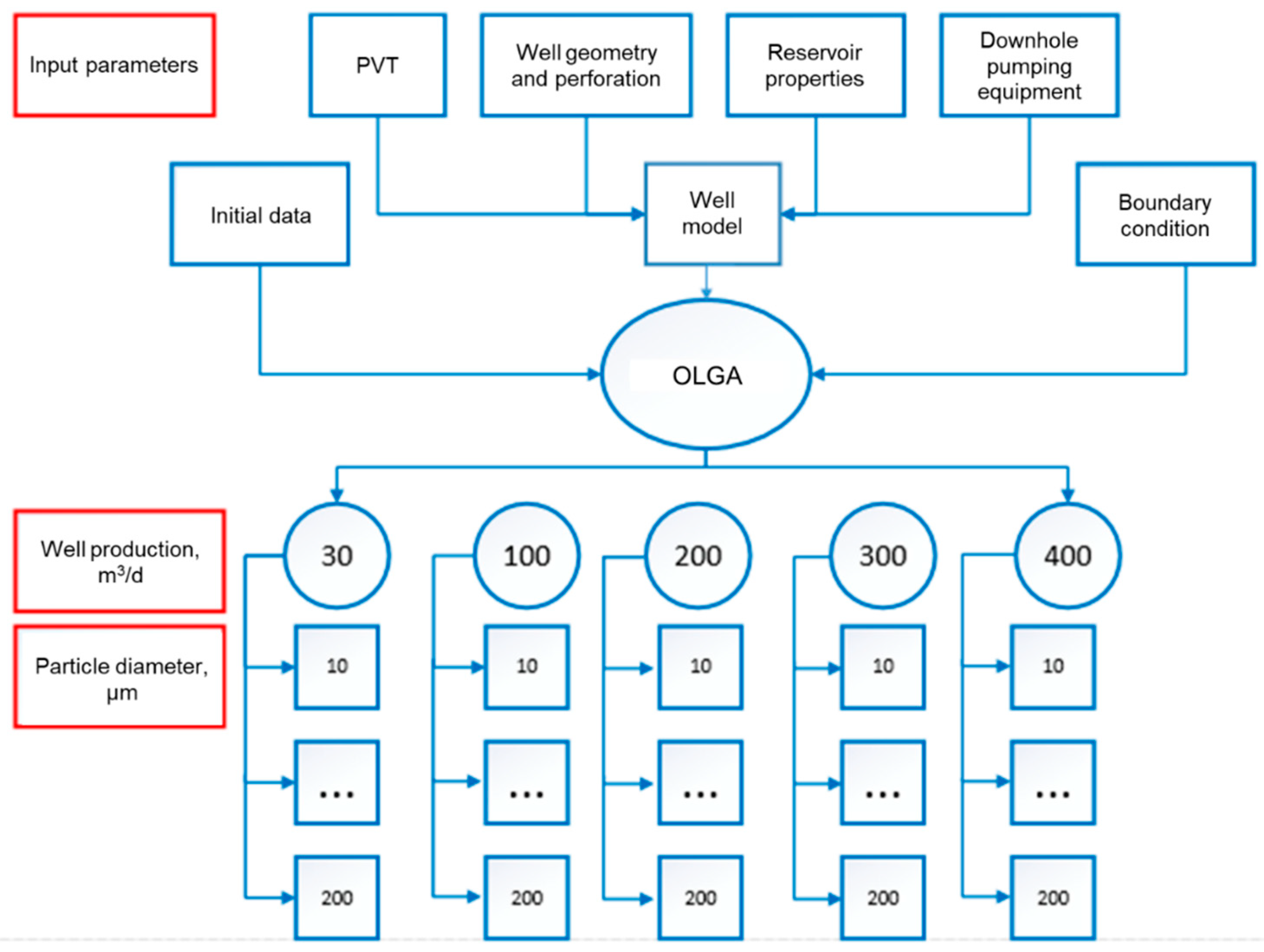
The research algorithm comprised the following (Figure 1). After the well model was created, the initial and cutoff temperatures and pressure conditions were set based on the input data. The calculations were made for 5 different production rates of the well: 30, 100, 200, 300, and 400 m3/d. Data on well operation with particles of a certain diameter (10 to 200 μm) were obtained for each production rate. In the OLGA software, there is no possibility to simulate a flow made of particles of different diameters. Therefore, each case was data on the behavior of particles of a selected diameter in a certain well flow rate. The time of simulation of each case (well flow rate and particle diameter) was 48 h per calculation time.
For calculation of the behavior of solid particles in the OLGA software, it was necessary to create an oil model based on composition. Oil for the «Training» field was modeled using Multiflash software [37]. The error in determining the dynamic viscosity did not exceed 10%, while for the bubble point pressure, it did not exceed 5%. S deviations could be considered satisfactory.
The main parameters of the product and reservoir of this field are presented in Table 1.
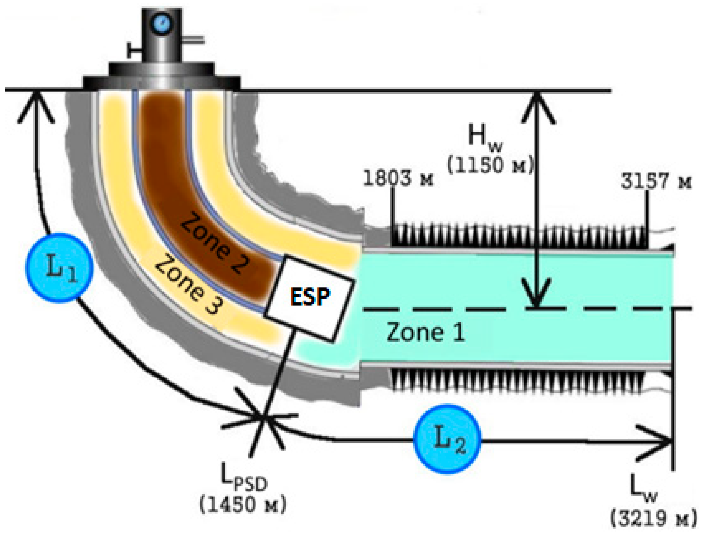
Figure 2 presents a scheme of the typical well on the «Training» field. To simplify the understanding of the processes of movement and accumulation of particles, the well was conventionally divided into 3 areas: horizontal borehole to the pump inlet, production tubing, and annulus. Particles of mechanical impurities appeared in zone 1 and were lifted out of the well via zone 2. In addition, the fraction of particles (sometimes significant) accumulated in zone 3; however, this phenomenon was not considered within the current work.
All calculations presented in this work were performed for a concentration of particles at the bottom of 250 mg/L (vol.: 0.011%)—average concentration of impurities in the flow during the operation of the studied field under steady state; density of particles was taken as 2300 kg/m3; and the watercut was 30%. It was assumed that particles moved to the bottom evenly over the entire perforation interval.
3. Results
Based on the obtained character of particle recovery, it was found that sand production could be of three types: stationary, quasi-steady, and burst, depending on well productivity and its structural features.
Stationary recovery is a recovery of particles in which their concentration in the flow does not depend on time. At the same time, it is not necessary that all particles that hit the bottom be removed. Some of them will settle and accumulate in the wellbore.
Quasi-steady recovery is recovery in which the concentration of particles in the flow is irregular and located at some value, changing randomly for low values. This is because sand may be transported both in a suspended state [38] and by “dragging” along the wellbore. Dabirian called this movement “mobile” dunes. If part of the sand passes from the suspended state into a “mobile” dune, then the concentration of particles in the fluid flow decreases; if a reverse phenomenon is observed (movement of sand from the dune into the fluid flow), the concentration of particles in the flow is increasing [39].
Burst recovery, in turn, differs from the second case, although there are some similarities. Similar to cyclic withdrawal, it is characterized by a non-constant concentration of particles in the flow in time. However, this is not due to passage of particles from one flow into another, but to accumulation at the bottom. Particles accumulate in the wellbore (predominantly at the entry point of the well trajectory into the formation) within a certain time, until they are strongly involved in the flow. There is an open question regarding the cause of the particles’ movement: narrowing of the penetration section, formation of local vortex, and instability of accumulation (local accumulation represents a cone made of sand, and the upper part of this figure is unstable and may collapse). In our opinion, several factors present an influence here simultaneously, but the degree of influence of one or another is currently a debatable issue.
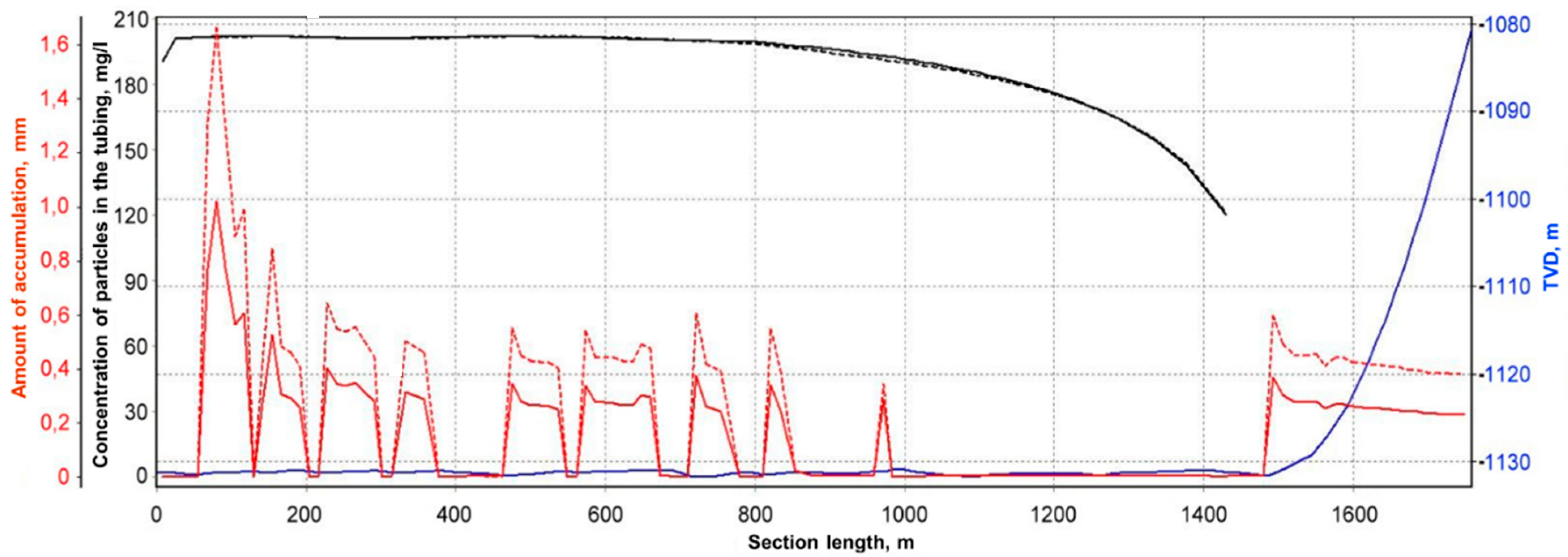
Figure 3 provides an example of stationary recovery. The specifics of this phenomenon are a constant concentration of particles inside the tubing in time and a continuous growth of the “pillow” (stationary layer) at the bottom hole. The chart must be read from left to right; it combines black lines for the tubing (schematically shown in Figure 3—L1), red lines for the section from the toe to the pump inlet (in Figure 3—L2), and a blue line for the bottom-hole profile (in Figure 3—3157–1803 m).
In Figure 3, the solid lines correspond to the moment at 12 h. As seen in the graph, a layer of particles was accumulated at the bottom of the hole equal to 0.3 mm, and the concentration of mechanical impurities in the flow in tubing was 190 mg/L. We concluded that 60 mg per each liter of sand was accumulated at the bottom hole. After 24 h, the fixed layer of particles at the bottom was 0.5 mm from the beginning of the calculation, while the concentration of particles in the tubing did not change and remained 190 mg/L. Figure 2 shows that more particles accumulated in the “toe” of the well than the “heel”. It should also be noted that accumulations were primarily localized in the “lowlands”—in those places where there were depressions in the well profile.
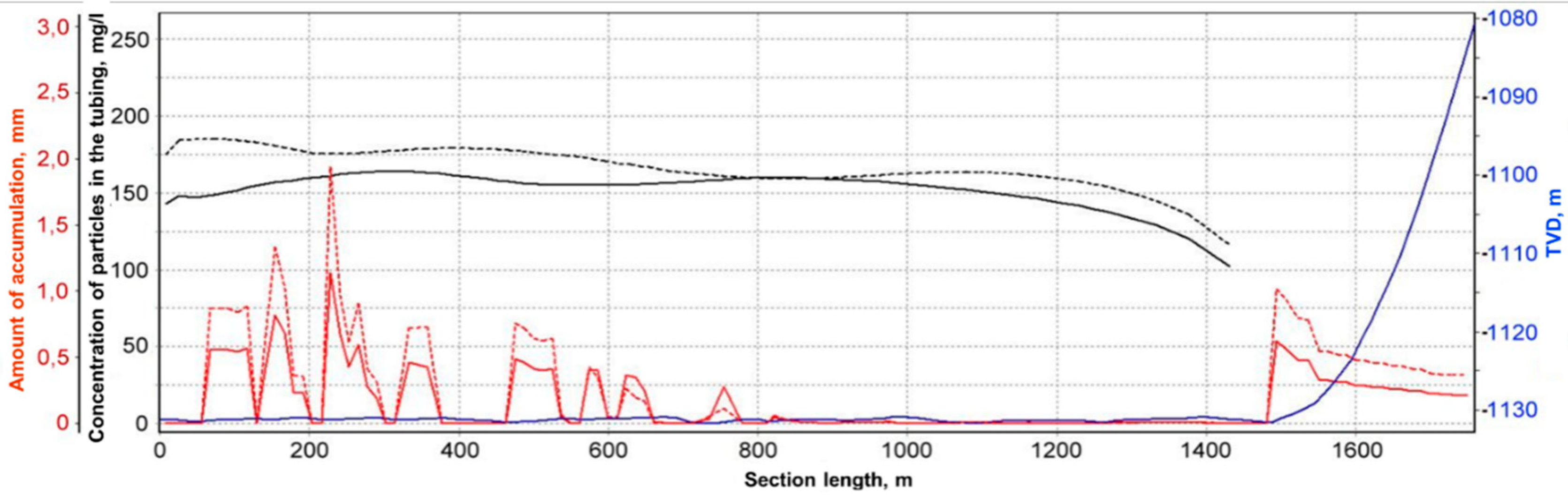
Figure 4 shows graphs featuring quasi-steady recovery. Its distinctive features are a random slight change in the particle concentration in the flow in time and uniform growth of the “pillow” at the bottom hole. The graph clearly shows that the concentration lines of particles in tubing (solid and dashed black lines) did not bend on each other, but lay close to 160 mg/L. Some sand was moving in the form of “mobile” dunes. This was because the flow rate was not enough to bring the particles into suspension, but it was enough to set them in motion along the wellbore.
The last type of withdrawal was a burst (Figure 5). It was caused by a large volume of particles accumulating at the place of well path entry into the formation, and then at a certain point in time, the majority of particles or cumulative volume were involved in the flow, leading to multiple growths in concentration. In the presented example, the number of particles in the flow increased by 7 times (dashed black line vs. solid black line). A low concentration of particles prior to the burst (black solid line) was associated with the fact that almost all sand accumulated in the well without falling into the tubing during formation of the sand dunes (red lines in the well “heel”). It can be seen that the main volume of particles before the burst was contained in the well “heel” (smooth red line), and these particles were involved in the flow during the burst (dashed red line).
One of the main objectives of the study was to determine the quality of particle recovery by fractions within the production rates of wells on the «Training» field. Quality of recovery means the ratio of particles that reached the wellhead to the total number of particles that arrived at the bottom.
Figure 6 shows recovery of particles of various diameters when the flow rate of the well was 200 m3/d. It became clear that with increased particle diameter, the type of withdrawal changed. Then the graph could be divided into three typical zones: zone 1—a zone of stationary and quasi-stationary recovery (at this rate, non-stationary recovery began with a particle diameter of 45 μm); zone 2—burst zone (where the quality of recovery was not possible to register); and zone 3—no recovery of particles.
Analogically to Figure 6, curves for other production rates were generated (Figure 7) that were within the production rates of operating company of the «Training» field. For example, if the well production rate was 100 m3/d and the diameter of particles was 30 μm, only 60% of particles from the total volume would be produced at the wellhead; for a production rate of 200 m3/d, the quality of recovery for particles of this diameter would be just below 80%. For each graph, the coefficient of determination had a value not lower than 0.98. The dashed lines indicate the critical diameters for the corresponding flow rate. The critical particle diameter was the diameter at which particles can no longer be carried from the bottom of the well to the wellhead. For example, at a production rate of 100 m3/d, particles with a diameter of 70 μm would not be recovered from the well, since a critical diameter for this production rate was 60 μm.
Practical application of the graphs in Figure 8 could be found when establishing the optimal mode of well operation, but was complicated by solids recovery. If this graph was compared with that of the volume of particles removed from the near-wellbore zone by fractions at different drawdowns, then it became clear what accumulation rate was expected in different well operation modes. Then, based on the production gain (when the bottom-hole pressure dropped), as well as the production losses due to well shut-in for sand cleanout expenses for implementation, the optimal operating conditions could be determined. This mode ensured the maximum possible production while taking into account cleanout of solids from the bottom hole (in fact, the optimal number of flushings per calendar period was determined).m3
The dependence between the well production rate and critical particle diameter is shown in Figure 8. This graph allows the presentation of the sizes of particles that could be withdrawn at the corresponding flow rate. As can be seen in Figure 8, there was a need for two different functions for approximation of the points. This was due to the fact that prior to a flow rate of 235 m3/day, the flow in the well was laminar, while afterward, it was transitional: in the laminar mode, the settling rate depended on the particle diameter through a quadratic dependence; and in the transitional mode, through a linear one.
This graph is important when choosing the separation fineness of down-hole filters. For example, there is no need to retain particles with a high recovery quality, but particles with a larger diameter should be reliably isolated from the bottom hole. The graph allows applying individual approaches to each well (depending on the production rate) to optimize production (reductions in hydraulic losses on the filter, as well as expenses for filter purchases).
As a result, it was also possible to answer the question regarding what fineness of separation to choose for the separator of an electrically driven vane pump installation. For example, if the production rate of the well is 50 m3/day, and the fineness of separation of the installed equipment is 100 μm, this does not make sense, since the critical diameter is 45 μm. Particles with a diameter of more than 100 μm cannot physically mobilize from the bottom hole.
Note: graphs 7 and 8 are only valid for a private case («Training» field), but can be used with some approximation in other fields with high-viscosity oil.
The results of previous studies correlated well with the data presented in the current article. The graphs [33] clearly showed that sand was actively accumulating in the lowlands of the wellbore trajectory. This was the result of the fact that moving dunes (moving cushion layer) could not overcome the rise and became stationary (fixed cushion layer). We can observe this phenomenon in Figure 3, Figure 4 and Figure 5. The main difference between our work and [33] is that we obtained a more active accumulation of particles in the place of a sharp change in the wellbore trajectory; whereas in [33], this phenomenon was observed only on the 38th day and was not so pronounced.
It was shown in [34] that with an increase in the particle diameter, sand removal deteriorated, which, in turn, was confirmed by us (Figure 7). The graphs clearly showed the degradation of the removal quality as the particle diameter increased. The difference from our work is that the authors of [34] conducted their study at higher well flow rates (about 1950 m3/day). In the vast majority of cases, impurities were in suspension, and there were no moving dunes (the moving part of the cushion). Nevertheless, ref. [34] clearly showed a significant accumulation of particles in the heel of the well, which was almost absent in [33].
The results of the work of R. Dabirian and team [35] are interesting from the point of view of comparing their obtained results with ours. In our work, we obtained similar results (Figure 7). It was also established in [35] that the modes could be combined: for example, dilute solids at wall, concentrated solids at wall, moving dunes, stationary dunes, and stationary bed. The point of contact between the study in [35] and ours was the fact that it was difficult to achieve the fully dispersed solid flow mode in practice in its pure form (Figure 7), since a small proportion of particles will always be located in the stationary part of the pillow (as was the case in our study). It should be noted that a distinctive feature of fully dispersed solid flow is that not a single particle comes into contact with the well wall. However, R. Dabirian and team still achieved a fully dispersed solid flow mode in [38]. The result was obtained in the laboratory setup described above at a low particle concentration and a high gas–liquid flow rate.
4. Conclusions
Within the framework of this study, a typical well model was created in the OLGA software, which made it possible to study and analyze the behavior of particles of mechanical impurities in horizontal wells with high-viscosity oil.
As a result of the calculations, it was found that depending on the value of parameters affecting the recovery process (production rate, diameter of particles), particle recovery can be stationary (Figure 2), quasi-steady (Figure 3), or burst (Figure 4).This phenomenon should be proved through laboratory experiments or during monitoring of the operation of real wells. If burst recovery really takes place in practice, then it is difficult to overestimate its danger to down-hole equipment.
The curves of quality of recovery (Figure 6) allowed for efficient selection of the optimum well operating mode (compared to the recovery data for formation particles), which will ensure minimization of the cost of production of a large quantity of oil, while taking into account the frequency of well interventions (well flushing).
Plotting of the critical particle diameter versus the flow rate (Figure 8) will allow optimal selection of down-hole filters and separator of mechanical impurities for electrically driven vane pumps.
This work is the first step in integrated studies of solid particle behavior in horizontal wells using the modern software OLGA and Multiflash. The value of these simulators in a professional environment and the quality of the analytical equations presented in them may indicate a high reliability of the results obtained.
Author Contributions
Conceptualization, A.D. and V.S.; methodology, A.P.; software, V.S.; formal analysis, E.S.; data curation, E.S.; writing—original draft preparation, V.S. and A.D.; writing—review and editing, A.P.; visualization, V.S.; supervision, A.D.; project administration, E.S. All authors have read and agreed to the published version of the manuscript.
Funding
This research received no external funding.
Conflicts of Interest
The authors declare no conflict of interest.
References
- Khakimova, S.; Nefedov, Y.; Nizamutdinova, I.; Shangaraeva, G.; Munasypov, R. Updating of the geological structure of the neocomian deposits within the novoportovskoye field during prospecting surveys. In Proceedings of the Saint Petersburg 2020-Geosciences: Converting Knowledge into Resources Conference Proceedings, Saint Petersburg, Russia, 16–19 November 2020; Volume 2020, pp. 1–5. [Google Scholar]
- Yassin, M.R.; Alinejad, A.; Asl, T.S.; Dehghanpour, H. Unconventional well shut-in and reopening: Multiphase gas-oil interactions and their consequences on well performance. J. Pet. Sci. Eng. 2022, 215, 110613. [Google Scholar] [CrossRef]
- Yurakv, V.; Dushina, V.; Mochaloval, A. Vs sustainable development: Scenarios for the future. J. Min. Inst. 2020, 242, 242. [Google Scholar] [CrossRef]
- Brilliant, L.S.; Dulkarnaev, M.R.; Danko, M.Y.; Lisheva, A.O.; Nabiev, D.K.; Khutornaya, A.I.; Malkov, I.N. Oil production management based on neural network optimization of well operation at the pilot project site of the Vatyeganskoe field (Territorial Production Enterprise Povkhneftegaz). Georesursy 2022, 24, 3–15. [Google Scholar] [CrossRef]
- Martyushev, D.A. Modeling and prediction of asphaltene-resin-paraffinic substances deposits in oil production wells. Georesursy 2020, 22, 86–92. [Google Scholar] [CrossRef]
- Lutome, M.S.; Lin, C.; Chunmei, D.; Zhang, X.; Bishanga, J.M. 3D geocellular modeling for reservoir characterization of lacustrine turbidite reservoirs: Submember 3 of the third member of the Eocene Shahejie Formation, Dongying depression, Eastern China. Pet. Res. 2022, 7, 47–61. [Google Scholar] [CrossRef]
- Tananykhin, D.; Korolev, M.; Stecyuk, I.; Grigorev, M. An investigation into current sand control methodologies taking into account geomechanical, field and laboratory data analysis. Resources 2021, 10, 125. [Google Scholar] [CrossRef]
- Galkin, V.I.; Martyushev, D.A.; Ponomareva, I.N.; Chernykh, I.A. Developing features of the nearbottomhole zones in productive formations at fields with high gas saturation of formation oil. J. Min. Inst. 2021, 249, 386–392. [Google Scholar] [CrossRef]
- Burenina, I.V.; Avdeeva, L.A.; Solovjeva, I.A.; Khalikova, M.A.; Gerasimova, M.V. Improving Methodological Approach to Measures Planning for Hydraulic Fracturing in Oil Fields. J. Min. Inst. 2019, 237, 343. [Google Scholar] [CrossRef]
- Mardashov, D.V.; Bondarenko, A.V.; Raupov, I.R. Technique for calculating technological parameters of non-Newtonian liquids injection into oil well during workover. J. Min. Inst. 2022. [Google Scholar] [CrossRef]
- Beloglazov, I.; Morenov, V.; Leusheva, E.; Gudmestad, O.T. Modeling of heavy-oil flow with regard to their rheological properties. Energies 2021, 14, 359. [Google Scholar] [CrossRef]
- Mayet, A.M.; Alizadeh, S.M.; Nurgalieva, K.S.; Hanus, R.; Nazemi, E.; Narozhnyy, I.M. Extraction of time-domain characteristics and selection of effective features using correlation analysis to increase the accuracy of petroleum fluid monitoring systems. Energies 2022, 15, 1986. [Google Scholar] [CrossRef]
- Penkov, G.M.; Karmansky, D.A.; Petrakov, D.G. Simulation of a fluid influx in complex reservoirs of western siberia. In Topical Issues of Rational use of Natural Resources-Proceedings of the International Forum-Contest of Young Researchers, Saint Petersburg, Russia, 13–17 May 2019; CRC Press: Boca Raton, FL, USA, 2019; pp. 119–124. [Google Scholar]
- Chen, X.; Paprouschi, A.; Elveny, M.; Podoprigora, D.; Korobov, G. A laboratory approach to enhance oil recovery factor in a low permeable reservoir by active carbonated water injection. Energy Rep. 2021, 7, 3149–3155. [Google Scholar] [CrossRef]
- Blatch, N.S. Discussion of «Works for the Purification of the Water Supply Washington DC»; Hazen, A.; Hardy, E.D., Translators; American Society of Civil Engineers: Reston, VA, USA, 1906; Volume 57, pp. 400–409. [Google Scholar]
- Durand, R.; Condolios, E. The Hydraulic Transportation of Coal and Solid Material in Pipes. In Proceedings of the Colloquium on Hydraulic Transport of Coal, National Coal Board, London, UK, 5 November 1952. [Google Scholar]
- Durand, R. Basic relationships of the transportation of solids in pipes experimental research. In Proceedings of the Minnesota Int. Hydraul. Convent, Minneapolis, MN, USA, 1–4 September 1953; pp. 89–103. [Google Scholar]
- Newitt, D.M.; Richardson, J.F.; Abbott, M.; Turtle, R.B. Hydraulic conveying of solids in horizontal pipes. Trans. Inst. Chem. Eng. 1955, 33, 93–113. [Google Scholar]
- Hughmark, G.A. Aqueous transport of settling slurries. Ind. Eng. Chem. 1961, 53, 389–390. [Google Scholar] [CrossRef]
- Thomas, D.G. Transport characteristics of suspensions part. Minimum transport velocity of flocculated suspensions in horizontal pipes. AIChE J. 1961, 7, 423–430. [Google Scholar] [CrossRef]
- Yang, Y.; Peng, H. Wen « Sand Transport and Deposition Behaviour in Subsea Pipelines for Flow Assurance». Energies 2019, 12, 4070. [Google Scholar] [CrossRef] [Green Version]
- Shook, C.A.; Schriek, W.; Smith, L.G. Husband «Experimental Studies of the Transport of Sands in Liquids of Varying Properties in 2- and 4-inch Pipelines»; Report E73-20; Saskatchewan Research Council: Saskatoon, SK, Canada, 1973. [Google Scholar]
- Wani, G.A. «Critical velocity in multisize particle transport through pipes». In Encyclopedia of Fluid Mechanics; Gulf Publishing Company: Houston, TX, USA, 1986; Volume 5, pp. 181–184. [Google Scholar]
- Gillies, R.G.; McKibben, M.J.; Shook, C.A. Pipeline flow of gas, liquid and sand mixtures at low velocities. J. Can. Pet. Tech. 1997, 36, 106. [Google Scholar] [CrossRef]
- Zorgania, E.; Al-Awadi, H.; Yan, W.; Al-lababid, S.; Yeung, H.; Fairhurst, C.P. Viscosity effects on sand flow regimes and transport velocity in horizontal pipelines. Exp. Therm. Fluid Sci. 2018, 92, 89–96. [Google Scholar] [CrossRef] [Green Version]
- Slepyan, F.B.; Cremaski, S.; Starika, S.; Subramani, H.J.; Cuba, G.E.; Gao, H. Confidence in critical velocity predictions for solid transport. In Proceedings of the Annual SPE Technical Conference and Exhibition, Amsterdam, The Netherlands, 27–29 October 2014. [Google Scholar] [CrossRef]
- Dabirian, R.; Mohammadiharkeshi, M.; Mohan, R.; Shoham, O. The critical rate of sand deposition in the evaluation of intermittent flow models. In Proceedings of the SPE Annual Technical Conference and Exhibition, Calgary, AB, Canada, 30 September–2 October 2019. [Google Scholar] [CrossRef]
- Oroskar, A.R.; Turian, R.M. The Critical Velocity in Pipeline Flow of Slurries. AIChE J. 1980, 26, 550–558. [Google Scholar] [CrossRef]
- Hill, A.L. Determining the Critical Flow Rates for Low Concentration Sand Transport in Two-Phase Pipe Flow by Experimentation and Modeling. Master’s Thesis, The University of Tulsa, Tulsa, OK, USA, 2011. [Google Scholar]
- Salama, M.M. Sand Production Management. J. Energy Resour. Technol. 2000, 122, 29–33. [Google Scholar] [CrossRef]
- Danielson, T.J. «Sand Transport Modeling in Multiphase Pipelines». In Proceedings of the 2007 Offshore Technology Conference, Houston, TX, USA, 30 April–3 May 2007. [Google Scholar]
- Schlumberger, The OLGA 2020User Manual, Version 2020.
- Liu, Y.; Jones, R.M.; Lu, H.; Putri, K.; Atmaca, S.; Gonzalez, N.J.R. A Multi-Factor Approach to Optimize Horizontal Shale Wells Flowback and Production Operation. In Proceedings of the SPE/AAPG/SEG Unconventional Resources Technology Conference, Houston, TX, USA, 26–28 July 2021. [Google Scholar]
- Ahmed, M. Transient Simulation Study of Well Trajectory Effect on Sand Transport in Multiphase Flow. In Proceedings of the SPE Annual Technical Conference and Exhibition, Virtual, 21–22 October 2020. [Google Scholar]
- Dabirian, R.; Mohan, R.; Shoham, O.; Kouba, G. Critical sand deposition velocity for gas-liquid stratified flow in horizontal pipes. J. Nat. Gas Sci. Eng. 2016, 33, 527–537. [Google Scholar] [CrossRef]
- Musi, A.; Larrey, D.; Monsma, J.; Paran, M.A.; Dekrin, M.K. «Selection, implementation and validation of a sand transportation model within a commercial multiphase dynamic simulator for effective sand management». In Proceedings of the 19th BHR International Conference on Multiphase Production Technology, Cannes, France, 5–7 June 2019. [Google Scholar]
- MultiflashTM, Infochem/KBC Process Technology Ltd. User Guide for Multiflash for Windows, Version 7.1; Kbc Advanced Technology Pte Ltd.: Singapore, 2020.
- Dabirian, R.; Mohan, R.S.; Shoham, O.; Kouba, G. Sand Transport in Stratified Flow in a Horizontal Pipeline. Paper presented at the SPE Annual Technical Conference and Exhibition, Houston, TX, USA, September 2015; pp. 2–4. [Google Scholar] [CrossRef]
- Shishulin, V.A. Development of Recommendations for Optimizing the Operation of Horizontal Wells in Conditions of Increased Removal of Mechanical Impurities. Master’s Thesis, Gubkin Russian State University of Oil and Gas (NRU), Moscow, Russia, 2021. [Google Scholar]
Figure 1.
Research algorithm.

Figure 2.
Schematic of the standard well on «Training» field.

Figure 3.
Stationary recovery of particles with diameter of 0.03 mm at rate of 200 m3/d: well geometry from toe to pump inlet (blue line), particle concentration in the flow in tubing (black lines), and accumulation of “pillow” from particles (red lines) at different moments in time: solid lines—12 h; dashed lines—24 h.

Figure 4.
Quasi-steady recovery of particles with diameter of 0.045 mm at rate of 200 m3/d: well geometry from toe to pump inlet (blue line), particle concentration in the flow in tubing (black lines), and accumulation of “pillow” from particles (red lines) at different moments in time: solid lines—7 h; dashed lines—14 h.

Figure 5.
Burst recovery of particles with diameter of 0.060 mm at rate of 200 m3/d: well geometry from toe to pump inlet (blue line), particle concentration in the flow in tubing (black lines), and accumulation of “pillow” from particles (red lines) at different moments in time: solid lines—9 h; dashed lines—10 h.

Figure 6.
Quality of recovery of solid particles by fractions at 200 m3/d.

Figure 7.
Quality of solids particles recovery by fractions at various well flow rates.

Figure 8.
Quality of solid particles recovery by fractions at various well flow rates.


Table 1.
Geological and physical summary of «Training» field.
| Parameter | Value | Parameter | Value |
|---|---|---|---|
| Reservoir | PK1 | Productivity index | 20–40 m3/day·MPa |
| Depth of occurrence | 1100–1150 m | Oil density in standard conditions | 917 kg/m3 |
| Reservoir temperature | 34 °C | Oil viscosity in situ | 67 mPa·s |
| Saturation pressure | 10.6 MPa | Oil viscosity in standard conditions | 860 mPa·s |
| Formation pressure | 10.6 MPa | Gas content | 32 m3/m3 |
Publisher’s Note: MDPI stays neutral with regard to jurisdictional claims in published maps and institutional affiliations. |
© 2022 by the authors. Licensee MDPI, Basel, Switzerland. This article is an open access article distributed under the terms and conditions of the Creative Commons Attribution (CC BY) license (https://creativecommons.org/licenses/by/4.0/).
Share and Cite
MDPI and ACS Style
Dengaev, A.; Shishulin, V.; Safiullina, E.; Palyanitsina, A. Modeling Results for the Real Horizontal Heavy-Oil-Production Well of Mechanical Solids. Energies 2022, 15, 5182. https://0-doi-org.brum.beds.ac.uk/10.3390/en15145182
AMA Style
Dengaev A, Shishulin V, Safiullina E, Palyanitsina A. Modeling Results for the Real Horizontal Heavy-Oil-Production Well of Mechanical Solids. Energies. 2022; 15(14):5182. https://0-doi-org.brum.beds.ac.uk/10.3390/en15145182
Chicago/Turabian StyleDengaev, Aleksey, Vladimir Shishulin, Elena Safiullina, and Aleksandra Palyanitsina. 2022. "Modeling Results for the Real Horizontal Heavy-Oil-Production Well of Mechanical Solids" Energies 15, no. 14: 5182. https://0-doi-org.brum.beds.ac.uk/10.3390/en15145182
Note that from the first issue of 2016, this journal uses article numbers instead of page numbers. See further details here.