Optimization of the Delivery Time within the Distribution Network, Taking into Account Fuel Consumption and the Level of Carbon Dioxide Emissions into the Atmosphere

Abstract

The evolution of changes in shopping in the modern society necessitates suppliers to seek new solutions consisting of increasing the efficiency of transport processes. When it comes to controlling the flow of goods in modern distribution networks, planning and timely deliveries are of particular importance. The first factor creating a competitive advantage involves the tendency to shorten order delivery times, especially for products with a short shelf life. Shorter delivery times, in turn, extend the period of effective residence of the product “available on the shelf”, increasing the likelihood of its sale. The second component in line with the Sustainable Development Strategy consists of aspects related to the protection of the natural environment, in particular those related to car transport. In this case, the fuel consumption and the level of emitted toxic substances (including carbon dioxide) are analyzed and assessed. Bearing in mind the above, this article presents the problem of optimizing the delivery time within the assumed distribution network and its solution, enabling the company to develop and optimal plan for the transport of products with a short shelf life. The paper proposes a model that takes into account minimization of the delivery time, while estimating the values of fuel consumption and CO₂ emissions for the variants considered. The means of transport were medium-duty trucks. Three variants of the assumptions were considered, and algorithms implemented in MS Excel and MATLAB software were used to perform the optimization. Using the MATLAB environment, a more favorable value of the objective function was obtained for the variant without additional constraints. On the other hand, the algorithm implemented in MS Excel more effectively searched the set of acceptable solutions with a larger number of constraining conditions.

1. Introduction

The issue of optimizing road transport considers a rich set of methods adapted to transport systems and has been widely described in scientific publications. The classic transport task is defined as the linear programming problem [1,2,3,4,5], which is the subject of a number of publications on new methods [6,7], algorithms [8], or on optimization techniques [9] of the existing decision node. Freight transport is often a decision problem in transport systems [10] affecting both the key performance indicators [11,12,13,14,15] and the level of customer service [16,17,18,19,20].

The set of trends shaping the current TSL (transport shipping logistics) industry includes [21] new business models (development of e-commerce, volatile customer purchasing habits, and a wide range of mobile payments), counselling and maintaining a high level of customer service (brand image building, the importance of social media, and linking the local brand with the global one), supply chains are drowning in data, businesses are going digital on a budget, precision of planning and timely deliveries (predictive models and push-e), and the tendency for supply chains to lengthen due to their global reach with a simultaneous tendency to shorten delivery times.

The significant pace of life, technological progress, and economic development increase customer requirements. According to a study [21], as many as 36% of buyers expect delivery the day after placing an order, 35% of customers would like to receive the goods up to two days after the transaction, while 11% of buyers would like to receive the goods on the same day. Therefore, the tendency to shorten delivery times is becoming an important element of competitiveness in the current flexible supply chains. The aforementioned tendency can be realized in many ways, i.e., by choosing the right means of transport, choosing the fastest and/or the shortest transport route [22,23], increasing the average speed of transport [24], efficient use of the vehicle’s loading area, eliminating empty runs [25,26], or effective prediction of flows within the distribution network [27,28,29]. The abovementioned possibilities essentially come down to optimization of the operating costs [30] of both private and public means of transport [31].

The literature, as part of research in the area of deliveries, presents various mathematical models concerning decision problems [23,28,32], as well as algorithms used to optimize transport processes [22,33,34,35]. For example, in [24,30], mathematical models simulating the functioning of delivery logistics systems were developed, enabling the determination of minimum logistics costs, assuming optimal delivery schedule arrangements (delivery sizes in subsequent periods of the project implementation). In contrast, in [36], the authors discussed the problem of shipping empty containers to meet the “on time delivery” requirements and moving other containers to terminals, warehouses, and cleaning stations. As a result of the research, a model for the optimization of this process was developed to improve the decision support process in conditions of uncertainty (lack of data) in order to more effectively manage the flow of empty containers within a predetermined planning horizon. The model includes practical aspects relating to the ECR distribution network (efficient consumer response), namely it meets the supply and demand requirements and deals with distribution costs, i.e., one of the main objectives of the ECR network. The aim of the research [22] was to optimize the transport of light petroleum products within gas stations located in urban agglomerations. In turn, in [37], the authors proposed a new criterion for the presented total costs, allowing for taking into account the direct costs of transport and losses related to the increase in delivery time. The presented mathematical model used to assess the reliability of transport has shown that the option of multimodal rail and sea transport of deliveries carried out in containers is the most rational, ensuring minimal transport costs with an acceptable order fulfilment time. On the other hand, the work of [38] presents a solution to the problem of routing multi-chamber vehicles for the needs of urban logistics. In order to minimize operating costs, the authors proposed an improved algorithm for searching large districts with routing [23,38,39]. The issues of the works of [40,41], in which the framework for supporting the decision-making process as part of improving the planning of current activities, have been developed. In addition, the issue of route optimization and the methodology for the rationalization of air transport were presented. On the other hand, Ref. [42] made the optimization of the transport service on demand. The problem was modelled as Dial-a-Ride, in which the set of user cost and inconvenience targets was optimized to accommodate naturally occurring constraints such as time windows and capacity.

In other publications, the authors, trying to improve the examined process or system, focused their attention on minimizing the selected cost components [43,44]; increasing the efficiency of the use of the vehicle fleet [45,46,47]; improvement of routing [48,49,50] in the area of city logistics; improved planning [51], design [52], and optimization of transport routes [53]; reduction of the emission of harmful substances to the natural environment [54,55,56]; minimizing delivery times [57] for “perishable” products [58]; and the possibility of using hydrogen in public transport systems [59].

In the above set of publications, attention was paid to the optimization of delivery time, fuel consumption, and carbon dioxide (CO₂) emissions, which are the subject of this study. The methodology proposed in this study was verified on the basis of the existing distribution network. If there are additional assumptions regarding the limited capacity of vehicles in a given decision problem, the presented algorithm should refer to the procedure based on the procedure developed for the problem of transport with limited route capacity. In the literature, the above procedure was used for small networks (i.e., 2 × 3—2 suppliers and 3 recipients, 3 × 4—3 suppliers and 4 recipients), while to solve a more complex decision problem, it is recommended to use IT software [60,61,62]. In the absence of IT (information technology) tools, an alternative is the solver add-on in the MS Excel spreadsheet. Its newer versions have much greater possibilities regarding the complexity (number of conditions and variables) of the decision problem, the type of functions used, and the time needed to solve it.

The structure of this article is presented below. Section 1 presents a literature review on the use of mathematical programming for the optimization of processes and systems. Section 2 describes the assumptions, the methodology of the procedure, and the construction of the mathematical model together with the algorithm of the procedure enabling the determination of the shortest transport time within the supply network. Section 3 describes how to apply the mathematical model on a numerical example related to the actual distribution network located in Poland. In Section 4, shows the analysis carried out on the total fuel consumption and CO₂ emissions to the atmosphere. Section 5 summarizes the results obtained and indicates the directions for further research.

2. Mathematical Model

In the publication, a model representing a closed transport task taking into account the time criterion was described with the following relations (1)–(6) [7,62,63,64,65]. The objective function, understood as the minimization of the maximum value of the product transport time on all available routes, was expressed by relation (1):

$$f\left(x_{n_i,m_j}\right)=\underset{x_{n_i,m_j}\ge 0}{\max }\left\{t_{ij}\right\}\to min,$$

(1)

where the value of the time taken to transport the product from delivery n_i to the consignee m_j is given by Formula (2):

$$t_{ij}=t_{ij}^p·\min \left\{x_{n_i,m_j},1\right\}+t_j^r·x_{n_i,m_j},$$

(2)

with limiting conditions relating to the supply (3) and demand (4), respectively:

$${{\displaystyle \sum }}_{j=1}^m{x}_{n_i,m_j}=a_i \left(i=1,\dots ,n\right),$$

(3)

$${{\displaystyle \sum }}_{i=1}^n{x}_{n_i,m_j}=b_j \left(j=1,\dots ,m\right),$$

(4)

and the non-negativity condition for decision variables (5):

$$x_{ij}\ge 0,$$

(5)

where

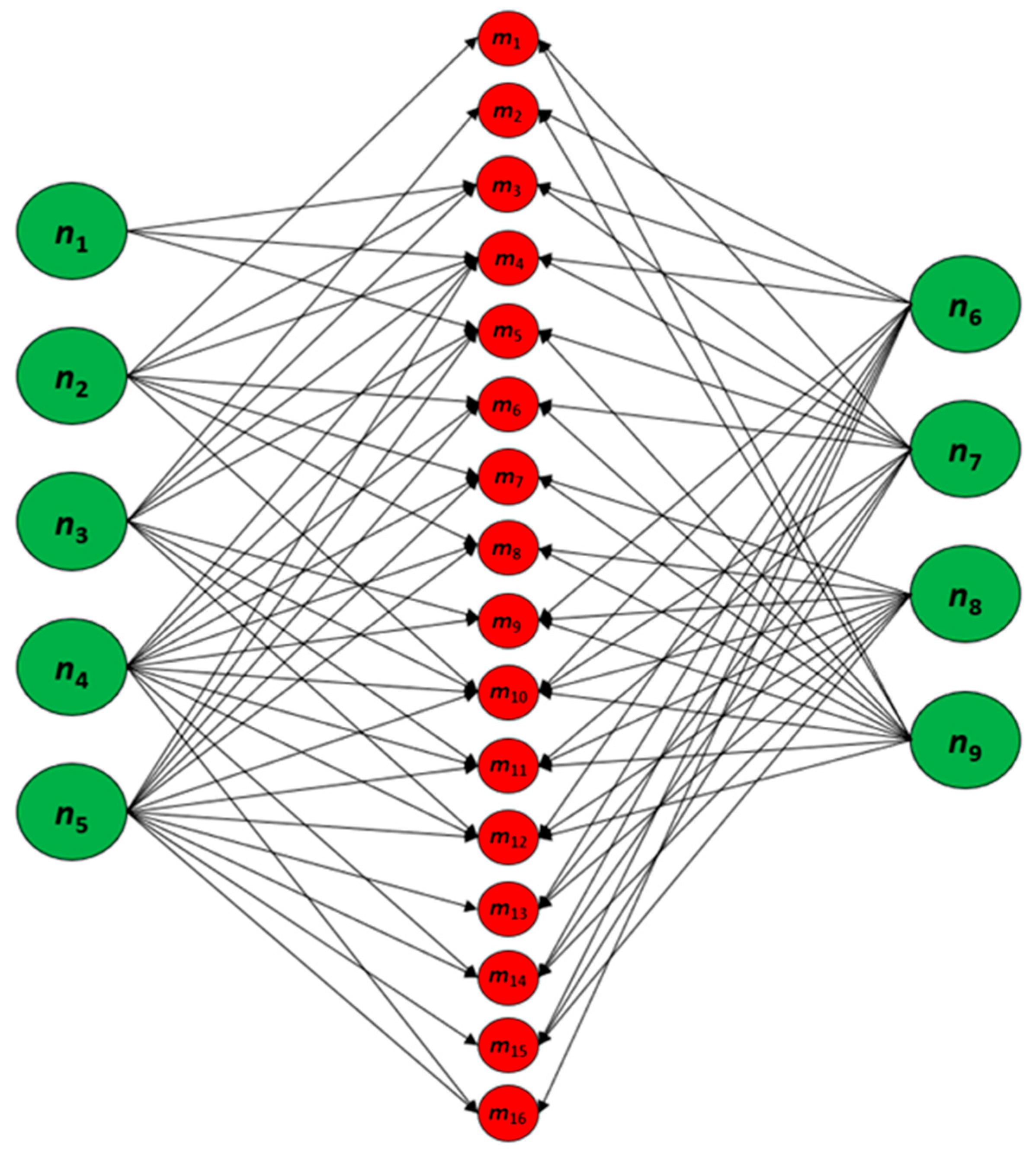
• $x_{n_i,m_j}$—number of load units of products with a short shelf-life delivered from the i-th supplier to the j-th recipient,
• t_ij—product transport time on the route from the i-th supplier to the j-th recipient,
• n—number of suppliers,
• m—number of recipients,
• a_i—supply of the i-th supplier,
• $b_j$—demand of the j-th recipient.

A closed transport task implies a balance between supply and demand, which is described by Formula (6):

$${{\displaystyle \sum }}_{i=1}^n{a}_i={{\displaystyle \sum }}_{j=1}^m{b}_j.$$

(6)

The above equations/inequalities (1)–(6) refer to the case of balancing the value of supply and demand (6). In a situation where the total demand and supply do not balance, relationship (6) takes the form of inequality. In this part of the publication, the calculations were carried out with the use of two software tools, i.e.,

• MS Excel spreadsheet,
• MATLAB software.

The procedure based on the use of the MS Excel capabilities is presented as the first one. The procedure algorithm based on iteration index k, which allows for building a model described by dependencies (1) ÷ (6), is presented in the following five steps:

• Determine the acceptable base solution using the method of the minimum matrix element [54] on the basis of the table with travel times.
• Determine the maximum delivery time (T^k) for the designated acceptable base solution on the basis of Formula (7):

$$T^k=\underset{x_{n_i,m_j}>0}{\max }\left\{t_{ij}\right\}$$

(7)

where $T^k$ is the maximum delivery time in the k-th iteration.

3.

Present the cost table (c_ij) for the k-th solution, using Formula (8):

$$c_{ij}=\left\{\begin{array}{c}0\\ 1\end{array} if \begin{array}{c}{t}_{ij}<T^k\\ t_{ij}=T^k\end{array}\right\}$$

(8)

4.

Determine from the $c_{ij}$ cost table whether the solution is optimal. In case the ${\Delta }_{ij}$ (9) optimality criteria are non-negative for all base routes, further calculations should be completed. Otherwise, go to step 5.

$${\Delta }_{ij}^k=c_{ij}^k-{\alpha }_i^k-{\beta }_j^k$$

(9)

where ${\alpha }_i^k$, ${\beta }_j^k$ are the dual variables (so-called potentials) in the k-th iteration.

5.

Determine a new acceptable base solution following the most negative optimality criterion, and then proceed to step 2.

The algorithm is graphically illustrated in Figure 1.

An alternative to MS Excel is the MATLAB programming environment, whose programming language is a high-level language with syntax modelled on the C language. In MATLAB, the surrogateopt function is used in the case of complex and time-consuming decision problems, and the solution requires finite boundaries for all variables, thus allowing nonlinear constraint inequalities as well as accepting integer constraints for selected variables [66].

The surrogateopt function is a global solver for time-consuming objective functions, which attempts to solve problems of the following form:

$$\underset{x_{n_i,m_j}}{\min }\left(\begin{array}{cc}f\left(x_{n_i,m_j}\right):& \{\begin{array}{c}l{b}_{ij}\le x_{n_i,m_j}\le u{b}_{ij}\\ c\left(x_{n_i,m_j}\right)\le 0\\ x_{n_i,m_j} \mathrm{integer}\end{array}\end{array}\right)$$

(10)

where $l{b}_{ij}$ and $u{b}_{ij}$ describe the lower and upper bound, respectively, of the decision value $x_{n_i,m_j}$, $c\left(x_{n_i,m_j}\right)$ means nonlinear constraints.

The solver searches for the global minimum of a real-valued objective function in multiple dimensions, subject to bounds, optional integer constraints, and optional nonlinear inequality constraints [67].

Surrogateopt is best suited to objective functions that take a long time to evaluate. The objective function can be non-smooth. The solver requires finite bounds on all of the variables. The solver can optionally maintain a checkpoint file to enable recovery from crashes or partial execution, or optimization continuation after meeting a stopping condition [66].

The procedure algorithm that allows for solving Equation (7) is described as follow:

• Create a set of trial points by sampling MinSurrogatePoints random points within the bounds, and evaluate the objective function at the trial points.
• Create a surrogate model of the objective function by interpolating a radial basis function through all of the random trial points.
• Create a merit function that gives some weight to the surrogate and to the distance from the trial points. Locate a small value of the merit function by randomly sampling the merit function in a region around the incumbent point (best point found since the last surrogate reset). Use this point, called the adaptive point, as a new trial point.
• Evaluate the objective at the adaptive point, and update the surrogate based on this point and its value. Count a “success” if the objective function value is sufficiently lower than the previous best (lowest) value observed, and count a “failure” otherwise.
• Update the dispersion of the sample distribution upwards if three successes occur before max(nvar,5) failures, where nvar is the number of dimensions. Update the dispersion downwards if max(nvar,5) failures occur before three successes.
• Continue from step 3 until all trial points are within MinSampleDistance of the evaluated points. At that time, reset the surrogate by discarding all adaptive points from the surrogate, reset the scale, and go back to step 1 to create MinSurrogatePoints new random trial points for evaluation.

3. Optimizing the Delivery Time within the Distribution Network—A Numerical Example and Results

The company specializes in the transport of products only within road transport. Cruises are carried out by identical means of transport that take place between the nodes of the network. The number of these points is fixed and strictly defined, and there is only service between them.

This article considers the distribution network including nodes located in the territory of the Republic of Poland. It consists of nine wholesalers (i.e., suppliers n₁, n₂, …, n₉) and 16 retail stores (i.e., recipients m₁, m₂, …, m₁₆) located geographically in voivodeship capital cities in Poland (Figure 2). The graph symbolizing the structure of the network reflecting all possible variants of transport is shown in Figure 3.

Table 1. Completion potential of suppliers.

a1	a2	a3	a4	a5	a6	a7	a8	a9
15	20	23	16	21	17	19	22	18

summarizes the individual picking potential of suppliers, while

Table 2. Demand of recipients.

b1	b2	b3	b4	b5	b6	b7	b8	b9	b10	b11	b12	b13	b14	b15	b16
12	9	7	15	9	10	12	10	18	9	6	12	6	6	8	9

shows the customers’ needs.

This article uses integer programming aimed at determining the optimal time of transporting products within the transport network consisting of a set of suppliers and recipients geographically located in Poland. The transport was carried out with the use of motor vehicles with a maximum permissible weight (MPW) of up to 3.5 tons. The technical data of the means of transport are summarized in

Table 3. Technical data of the transport means [68].

Vehicle	Mercedes-Benz
Model of vehicle	Vito W639 Furgon
Year of production	2009
Displacement	2148.0 cm3
Engine type	Diesel
Fuel consumption (average consumption)	8.6 l/100 km
Exhaust emissions (CO2 emissions)	229.0 g/km
Max. total vehicle weight (fully laden)	2770.0 kg

.

The total delivery time consists of the transport time from the warehouse to the given collection point and the handling time (including loading and unloading).

Table 4. Distance between suppliers and recipients (km).

	n1	n2	n3	n4	n5	n6	n7	n8	n9
m1	120	240	420	360	420	660	360	840	780
m2	360	120	60	180	360	420	600	660	600
m3	300	420	480	300	300	540	120	720	540
m4	360	300	300	180	120	420	180	540	540
m5	360	180	180	60	180	360	300	540	480
m6	480	480	480	300	120	480	60	600	360
m7	540	300	120	180	360	300	600	480	540
m8	840	540	360	360	480	180	660	300	480
m9	660	480	300	240	240	120	420	240	300
m10	540	420	360	180	120	240	300	360	360
m11	720	600	480	360	240	240	420	240	120
m12	840	660	480	420	420	120	540	60	240
m13	600	660	600	360	180	420	180	540	300
m14	660	660	540	360	240	420	240	420	180
m15	780	720	600	420	300	360	360	360	120
m16	900	780	600	480	480	300	480	180	120

summarizes the distances between the nodes of the supply network. Based on the average speed of transport on individual roads, taking into account the distance, in

Table 5. Travel time $t_{ij}^p$ (h).

	n1	n2	n3	n4	n5	n6	n7	n8	n9
m1	2	4	7	6	7	11	6	14	13
m2	6	2	1	3	6	7	10	11	10
m3	5	7	8	5	5	9	2	12	9
m4	6	5	5	3	2	7	3	9	9
m5	6	3	3	1	3	6	5	9	8
m6	8	8	8	5	2	8	1	10	6
m7	9	5	2	3	6	5	10	8	9
m8	14	9	6	6	8	3	11	5	8
m9	11	8	5	4	4	2	7	4	5
m10	9	7	6	3	2	4	5	6	6
m11	12	10	8	6	4	4	7	4	2
m12	14	11	8	7	7	2	9	1	4
m13	10	11	10	6	3	7	3	9	5
m14	11	11	9	6	4	7	4	7	3
m15	13	12	10	7	5	6	6	6	2
m16	15	13	10	8	8	5	8	3	2

, the travel times were calculated and the unit unloading times were calculated (

Table 6. The unit unloading time $t_j^r$ (h).

m1	m2	m3	m4	m5	m6	m7	m8	m9	m10	m11	m12	m13	m14	m15	m16
$\frac{1}{3}$	$\frac{1}{3}$	$\frac{1}{6}$	$\frac{1}{2}$	$\frac{1}{3}$	$\frac{1}{3}$	$\frac{1}{3}$	$\frac{1}{3}$	$\frac{2}{3}$	$\frac{1}{3}$	$\frac{1}{6}$	$\frac{1}{2}$	$\frac{1}{6}$	$\frac{1}{6}$	$\frac{1}{3}$	$\frac{1}{3}$

) at individual collection points. The differences in unloading times result from the heterogenous, in terms of the parameters of the unloading equipment, available at individual collection points.

The numerical example presented in this publication is a more complicated issue than the traditional transport problem with the time criterion, as it includes a network of 9 suppliers and 16 recipients. For this reason, the description of the optimization task only partially resembles the general mathematical model. In the case under consideration, the objective function assumes a complex and atypical form. Its fragment describes the following relationship (11):

$$\begin{array}{c}\max \{\left(2·\min \left\{x_{n_1,m_1},1\right\}+\frac{1}{3}{x}_{n_1,m_1}\right), \left(6·\min \left\{x_{n_1,m_2},1\right\}+\frac{1}{3}{x}_{n_1,m_2}\right),(5·\min \left\{x_{n_1,m_3},1\right\}\hfill \\ \hfill +\frac{1}{6}{x}_{n_1,m_3}), \left(6·\min \left\{x_{n_1,m_4},1\right\}+\frac{1}{2}{x}_{n_1,m_4}\right), (6·\min \left\{x_{n_1,m_5},1\right\}\hfill \\ \hfill +\frac{1}{3}{x}_{n_1,m_5}),\left(8·\min \left\{x_{n_1,m_6},1\right\}+\frac{1}{3}{x}_{n_1,m_6}\right),\dots ,(2·\min \left\{x_{n_9,m_{15}},1\right\}\hfill \\ \hfill +\frac{1}{3}{x}_{n_9,m_{15}}), \left(2·\min \left\{x_{n_9,m_{16}},1\right\}+\frac{1}{3}{x}_{n_9,m_{16}}\right) \}\to \min \hfill \end{array}$$

(11)

In addition, the model takes into account the limiting conditions (12) resulting from the demand of individual recipients:

$$\begin{array}{r}{x}_{n_1,m_1}+x_{n_2,m_1}+x_{n_3,m_1}+x_{n_4,m_1}+x_{n_5,m_1}+x_{n_6,m_1}+x_{n_7,m_1}+x_{n_8,m_1}+x_{n_9,m_1}=12\\ x_{n_1,m_2}+x_{n_2,m_2}+x_{n_3,m_2}+x_{n_4,m_2}+x_{n_5,m_2}+x_{n_6,m_2}+x_{n_7,m_2}+x_{n_8,m_2}+x_{n_9,m_2}=9\\ x_{n_1,m_3}+x_{n_2,m_3}+x_{n_3,m_3}+x_{n_4,m_3}+x_{n_5,m_3}+x_{n_6,m_3}+x_{n_7,m_3}+x_{n_8,m_3}+x_{n_9,m_3}=7\\ x_{n_1,m_4}+x_{n_2,m_4}+x_{n_3,m_4}+x_{n_4,m_4}+x_{n_5,m_4}+x_{n_6,m_4}+x_{n_7,m_4}+x_{n_8,m_4}+x_{n_9,m_4}=15\\ x_{n_1,m_5}+x_{n_2,m_5}+x_{n_3,m_5}+x_{n_4,m_5}+x_{n_5,m_5}+x_{n_6,m_5}+x_{n_7,m_5}+x_{n_8,m_5}+x_{n_9,m_5}=9\\ x_{n_1,m_6}+x_{n_2,m_6}+x_{n_3,m_6}+x_{n_4,m_6}+x_{n_5,m_6}+x_{n_6,m_6}+x_{n_7,m_6}+x_{n_8,m_6}+x_{n_9,m_6}=10\\ x_{n_1,m_7}+x_{n_2,m_7}+x_{n_3,m_7}+x_{n_4,m_7}+x_{n_5,m_7}+x_{n_6,m_7}+x_{n_7,m_7}+x_{n_8,m_7}+x_{n_9,m_7}=12\\ x_{n_1,m_8}+x_{n_2,m_8}+x_{n_3,m_8}+x_{n_4,m_8}+x_{n_5,m_8}+x_{n_6,m_8}+x_{n_7,m_8}+x_{n_8,m_8}+x_{n_9,m_8}=10\\ x_{n_1,m_9}+x_{n_2,m_9}+x_{n_3,m_9}+x_{n_4,m_9}+x_{n_5,m_9}+x_{n_6,m_9}+x_{n_7,m_9}+x_{n_8,m_9}+x_{n_9,m_9}=18\\ x_{n_1,m_{10}}+x_{n_2,m_{10}}+x_{n_3,m_{10}}+x_{n_4,m_{10}}+x_{n_5,m_{10}}+x_{n_6,m_{10}}+x_{n_7,m_{10}}+x_{n_8,m_{10}}+x_{n_9,m_{10}}=9\\ x_{n_1,m_{11}}+x_{n_2,m_{11}}+x_{n_3,m_{11}}+x_{n_4,m_{11}}+x_{n_5,m_{11}}+x_{n_6,m_{11}}+x_{n_7,m_{11}}+x_{n_8,m_{11}}+x_{n_9,m_{11}}=6\\ x_{n_1,m_{12}}+x_{n_2,m_{12}}+x_{n_3,m_{12}}+x_{n_4,m_{12}}+x_{n_5,m_{12}}+x_{n_6,m_{12}}+x_{n_7,m_{12}}+x_{n_8,m_{12}}+x_{n_9,m_{12}}=12\\ x_{n_1,m_{13}}+x_{n_2,m_{13}}+x_{n_3,m_{13}}+x_{n_4,m_{13}}+x_{n_5,m_{13}}+x_{n_6,m_{13}}+x_{n_7,m_{13}}+x_{n_8,m_{13}}+x_{n_9,m_{13}}=6\\ x_{n_1,m_{14}}+x_{n_2,m_{14}}+x_{n_3,m_{14}}+x_{n_4,m_{14}}+x_{n_5,m_{14}}+x_{n_6,m_{14}}+x_{n_7,m_{14}}+x_{n_8,m_{14}}+x_{n_9,m_{14}}=6\\ x_{n_1,m_{15}}+x_{n_2,m_{15}}+x_{n_3,m_{15}}+x_{n_4,m_{15}}+x_{n_5,m_{15}}+x_{n_6,m_{15}}+x_{n_7,m_{15}}+x_{n_8,m_{15}}+x_{n_9,m_{15}}=8\\ x_{n_1,m_{16}}+x_{n_2,m_{16}}+x_{n_3,m_{16}}+x_{n_4,m_{16}}+x_{n_5,m_{16}}+x_{n_6,m_{16}}+x_{n_7,m_{16}}+x_{n_8,m_{16}}+x_{n_9,m_{16}}=9\end{array}$$

(12)

and assumptions (13) regarding the supply of a network of suppliers (wholesalers):

$$\begin{array}{c}{x}_{n_1,m_1}+x_{n_1,m_2}+x_{n_1,m_3}+x_{n_1,m_4}+x_{n_1,m_5}+x_{n_1,m_6}+x_{n_1,m_7}+x_{n_1,m_8}+x_{n_1,m_9}+x_{n_1,m_{10}}\hfill \\ \hfill +x_{n_1,m_{11}}+x_{n_1,m_{12}}+x_{n_1,m_{13}}+x_{n_1,m_{14}}+x_{n_1,m_{15}}+x_{n_1,m_{16}}\le 15\hfill \\ x_{n_2,m_1}+x_{n_2,m_2}+x_{n_2,m_3}+x_{n_2,m_4}+x_{n_2,m_5}+x_{n_2,m_6}+x_{n_2,m_7}+x_{n_2,m_8}+x_{n_2,m_9}+x_{n_2,m_{10}}\hfill \\ \hfill +x_{n_2,m_{11}}+x_{n_2,m_{12}}+x_{n_2,m_{13}}+x_{n_2,m_{14}}+x_{n_2,m_{15}}+x_{n_2,m_{16}}\le 20\hfill \\ x_{n_3,m_1}+x_{n_3,m_2}+x_{n_3,m_3}+x_{n_3,m_4}+x_{n_3,m_5}+x_{n_3,m_6}+x_{n_3,m_7}+x_{n_3,m_8}+x_{n_3,m_9}+x_{n_3,m_{10}}\hfill \\ \hfill +x_{n_3,m_{11}}+x_{n_3,m_{12}}+x_{n_3,m_{13}}+x_{n_3,m_{14}}+x_{n_3,m_{15}}+x_{n_3,m_{16}}\le 23\hfill \\ x_{n_4,m_1}+x_{n_4,m_2}+x_{n_4,m_3}+x_{n_4,m_4}+x_{n_4,m_5}+x_{n_4,m_6}+x_{n_4,m_7}+x_{n_4,m_8}+x_{n_4,m_9}+x_{n_4,m_{10}}\hfill \\ \hfill +x_{n_4,m_{11}}+x_{n_4,m_{12}}+x_{n_4,m_{13}}+x_{n_4,m_{14}}+x_{n_4,m_{15}}+x_{n_4,m_{16}}\le 16\hfill \\ x_{n_4,m_1}+x_{n_4,m_2}+x_{n_4,m_3}+x_{n_4,m_4}+x_{n_4,m_5}+x_{n_4,m_6}+x_{n_4,m_7}+x_{n_4,m_8}+x_{n_4,m_9}+x_{n_4,m_{10}}\hfill \\ \hfill +x_{n_4,m_{11}}+x_{n_4,m_{12}}+x_{n_4,m_{13}}+x_{n_4,m_{14}}+x_{n_4,m_{15}}+x_{n_4,m_{16}}\le 16\hfill \\ x_{n_5,m_1}+x_{n_5,m_2}+x_{n_5,m_3}+x_{n_5,m_4}+x_{n_5,m_5}+x_{n_5,m_6}+x_{n_5,m_7}+x_{n_5,m_8}+x_{n_5,m_9}+x_{n_5,m_{10}}\hfill \\ \hfill +x_{n_5,m_{11}}+x_{n_5,m_{12}}+x_{n_5,m_{13}}+x_{n_5,m_{14}}+x_{n_5,m_{15}}+x_{n_5,m_{16}}\le 21\hfill \\ x_{n_6,m_1}+x_{n_6,m_2}+x_{n_6,m_3}+x_{n_6,m_4}+x_{n_6,m_5}+x_{n_6,m_6}+x_{n_6,m_7}+x_{n_6,m_8}+x_{n_6,m_9}+x_{n_6,m_{10}}\hfill \\ \hfill +x_{n_6,m_{11}}+x_{n_6,m_{12}}+x_{n_6,m_{13}}+x_{n_6,m_{14}}+x_{n_6,m_{15}}+x_{n_6,m_{16}}\le 17\hfill \\ x_{n_7,m_1}+x_{n_7,m_2}+x_{n_7,m_3}+x_{n_7,m_4}+x_{n_7,m_5}+x_{n_7,m_6}+x_{n_7,m_7}+x_{n_7,m_8}+x_{n_7,m_9}+x_{n_7,m_{10}}\hfill \\ \hfill +x_{n_7,m_{11}}+x_{n_7,m_{12}}+x_{n_7,m_{13}}+x_{n_7,m_{14}}+x_{n_7,m_{15}}+x_{n_7,m_{16}}\le 19\hfill \\ x_{n_8,m_1}+x_{n_8,m_2}+x_{n_8,m_3}+x_{n_8,m_4}+x_{n_8,m_5}+x_{n_8,m_6}+x_{n_8,m_7}+x_{n_8,m_8}+x_{n_8,m_9}+x_{n_8,m_{10}}\hfill \\ \hfill +x_{n_8,m_{11}}+x_{n_8,m_{12}}+x_{n_8,m_{13}}+x_{n_8,m_{14}}+x_{n_8,m_{15}}+x_{n_8,m_{16}}\le 22\hfill \\ x_{n_9,m_1}+x_{n_9,m_2}+x_{n_9,m_3}+x_{n_9,m_4}+x_{n_9,m_5}+x_{n_9,m_6}+x_{n_9,m_7}+x_{n_9,m_8}+x_{n_9,m_9}+x_{n_9,m_{10}}\hfill \\ \hfill +x_{n_9,m_{11}}+x_{n_9,m_{12}}+x_{n_9,m_{13}}+x_{n_9,m_{14}}+x_{n_9,m_{15}}+x_{n_9,m_{16}}\le 18\hfill \end{array}$$

(13)

as well as condition (14), referring to the integer nature of decision variables:

$$x_{n_1,m_1},x_{n_1,m_2},\dots ,x_{n_9,m_{16}}\in N$$

(14)

where

• $x_{n_1,m_1}$—number of sets transported from the sender n₁ to the recipient m₁,
• $⋮$
• $x_{n_9,m_{16}}$—number of sets transported from the sender n₉ to the recipient m₁₆.

The type of route was determined in relations to (15). If the rounded quotient assumes a value close to 1.0, the analyzed route is defined as the base route. On the other hand, the zero value of the quotient indicates a non-basic route, i.e., one on which there will be in fact no transport.

$$\frac{x_{n_i,m_j}}{x_{n_i,m_j}+0.00001}$$

(15)

Using the presented method, in the final stage, only the times related to the base routes should be taken into account for further analyses.

The data summarized in Table 4, Table 5 and Table 6, the limiting conditions relating to demand described in Equation (12), and the supply assumptions presented in Equation (13) formed the basis for the calculations performed in the MS Excel spreadsheet. The longest delivery time of 15 h occurred in the m₁₆-n₁ relation (see Table 5). In the case under consideration, it should be interpreted as the initial baseline solution.

Using the dependence (1)–(6) and the condition from Equation (14), as a result of the performed calculations, the optimal solution was obtained, amounting to 13.3 h. The values of the decision variables (the number of cruises on individual routes) are summarized in

Table 7. Values of decision variables (Variant #1, MS Excel).

	n1	n2	n3	n4	n5	n6	n7	n8	n9
m1	0	6	0	0	0	0	5	0	1
m2	0	0	6	0	0	2	0	0	1
m3	1	1	3	0	0	1	1	0	0
m4	5	1	3	1	2	1	2	0	0
m5	1	0	2	1	1	0	1	0	3
m6	0	3	0	1	1	0	4	0	1
m7	0	4	0	1	2	0	0	2	3
m8	0	1	0	1	2	0	0	3	3
m9	0	0	3	3	0	4	0	5	3
m10	1	0	1	1	1	1	1	2	1
m11	0	0	1	1	1	0	1	1	1
m12	0	0	2	2	1	2	0	4	1
m13	0	0	0	0	1	1	1	2	0
m14	0	0	0	2	1	1	1	1	0
m15	0	0	0	0	2	2	2	2	0
m16	0	0	0	1	6	2	0	0	0

.

The presented decision problem was solved using the MATLAB software (surrogateopt function). In this case, it was necessary to modify and introduce additional restrictions on the decision variables. Conditions (1)–(6) remained unchanged. According to the general relationship (10), Equation (4) has been replaced by two inequalities:

$$\left(b_j-0.5\right)\le {\displaystyle \sum }_{i=1}^n{x}_{n_i,m_j}\le b_j \left(j=1,\dots ,m\right)$$

(16)

The lower bound of $l{b}_{ij}=0$ was adopted, which corresponds to condition (5), and the upper bound $x_{n_i,m_j}\le u{b}_{ij}$, which is mandatory in MATLAB software (Mathworks Inc., Natick, MA, USA) for the surrogateopt function, was added. The optimization was carried out for the same assumptions as those adopted in the solution obtained with the use of the solver add-on.

1.

Variant #1: it was assumed that the decision variables cannot be greater than the corresponding demand and supply. It was written as dependence (17):

$$u{b}_{ij}=min\left(a_i,b_j\right) \left(i=1,\dots ,n\right), \left(j=1,\dots ,m\right)$$

(17)

For Variant #1, the delivery lead time was 12.72 h. The decision variables values are summarized in

Table 8. Values of decision variables (Variant #1, MATLAB).

	n1	n2	n3	n4	n5	n6	n7	n8	n9
m1	12	0	0	0	0	0	0	0	0
m2	0	1	0	0	0	0	0	0	8
m3	0	6	0	0	0	0	0	0	0
m4	0	0	0	1	3	0	11	0	0
m5	0	0	9	0	0	0	0	0	0
m6	0	0	0	10	0	0	0	0	0
m7	0	0	0	0	12	0	0	0	0
m8	0	10	0	0	0	0	0	0	0
m9	0	1	0	0	0	16	0	1	0
m10	0	2	8	0	0	0	0	0	0
m11	0	0	0	5	0	0	1	0	0
m12	0	0	0	0	0	0	0	11	1
m13	0	0	0	0	5	0	0	0	0
m14	0	0	6	0	0	0	0	0	0
m15	0	0	0	0	0	0	0	8	0
m16	0	0	0	0	0	0	0	0	9

.

In the next step, the average value of the decision variables included in Table 8 was calculated, which was $x_{n_i,m_j}$ = 8. In order to narrow down the set of acceptable base solutions, Table 8 searched for a value lower than the mean and at the same time the closest value of the decision variable $x_{n_i,m_j}$ = 6. On the basis of these two values of the decision variable, additional constraints were formulated by considering the two described variants, i.e.,

2.

Variant #2: it was assumed that decision variables cannot be greater than the respective demand and supply and the mean value of the decision variable $x_{n_i,m_j}$ = 8 calculated from the tale, which is written as:

$$u{b}_{ij}=min\left(a_i,b_j,8\right) \left(i=1,\dots ,n\right), \left(j=1,\dots ,m\right)$$

(18)

3.

Variant #3: it was assumed that the decision variables cannot be greater than the respective demand and supply, and the value $x_{n_i,m_j}$ = 6 is lower, but it is closest to the calculated mean, according to (16):

$$u{b}_{ij}=min\left(a_i,b_j,6\right) \left(i=1,\dots ,n\right), \left(j=1,\dots ,m\right)$$

(19)

As a result of the performed calculations, graphs of the function values depending on the number of iterations were obtained, which are presented for Variant #1 (Figure 4), Variant #2 (Figure 5), and Variant #3 (Figure 6).

Comparing the three considered variants obtained with the use of MATLAB software, it should be stated that the shortest delivery time of 12.34 h was obtained for Variant #2. Compared with the initial base solution (MS Excel) of 15 h, the result is 2.7 h less (time reduction by 18%). When analyzing Variant #1 and Variant #3 (MATLAB), it should be stated that the total delivery times are also shorter than the initial base solution (MS Excel) and are 12.72 (Variant #1) and 13.98 (Variant #3) h, respectively. In order to compare the above-obtained solutions, additional calculations were performed using MS Excel for the same constraints. After taking into account the condition relating to the decision variables, analogous to that in MATLAB, i.e., $x_{n_i,m_j}\le 8$, a solution of 9.3 h was obtained (

Table 9. Comparison of the results of the delivery time for the three variants.

	Variant #1	Variant #2	Variant #3
MS Excel (h)	13.3	9.3	9.0
MATLAB (h)	12.72	12.34	13.98

, Variant #2, MS Excel). In the next case, an equivalent constraint was imposed, assuming that the decision variables cannot be greater than the highest value obtained for MATLAB for Variant #3, i.e., $x_{n_i,m_j}\le 6$. After the calculations, the objective function value of 9.0 h was obtained, which is the optimal result (Table 9, Variant #3, MS Excel). The results obtained for both tools mentioned above, with the same assumptions, are summarized in Table 9.

When analyzing the results presented in Table 9, it should be stated that the time calculated using MATLAB was shorter compared to the solution obtained using MS Excel only for Variant #1. When comparing the results obtained for Variant #2 and Variant #3, MS Excel turned out to be a more effective tool. Introducing additional restrictions on the value of the decision variables naturally reduces the space of potential solutions. Both algorithms randomly search the set of acceptable base solutions, from which they adopt the best, consistent with the optimization direction (min/max). As the results obtained in Table 9 show, MATLAB is a more effective tool in the case of searching for a large number of sets of feasible solutions (Variant #1), while the use of MS Excel gives better results in the situation of narrowing the space of feasible solutions (Variant #2 and Variant #3).

4. Analysis of Fuel Consumption and the Level of CO₂ Emissions to the Atmosphere

On 25 September 2015 in New York, all 193 UN member states adopted the 2030 Agenda for Sustainable Development [69], including the Sustainable Development Goals, by the General Assembly. The Agenda defines 17 goals and 169 targets that should be achieved by 2030. They concern five areas, i.e., people, planet, prosperity, peace, and partnership. The goals cover a wide range of challenges such as poverty, hunger, health, education, gender equality, peace, and social justice, as well as climate change and sustainable development. The concept of sustainable development also includes sustainable transport. This means that not only social and economic criteria should be taken into account when planning transport, but also environmental aspects. Considering the above, in this part of the article, an analysis of fuel consumption was carried out and the level of CO₂ emissions into the atmosphere was determined. The input data were the solutions obtained with the use of MS Excel.

Table 10. Transport travel matrix for Variant #1.

	m1	m2	m3	m4	m5	m6	m7	m8	m9	m10	m11	m12	m13	m14	m15	m16
n1	0	0	1	1	1	0	0	0	0	1	0	0	0	0	0	0
n2	1	0	1	1	0	1	1	1	0	0	0	0	0	0	0	0
n3	0	1	1	1	1	0	0	0	1	1	1	1	0	0	0	0
n4	0	0	0	1	1	1	1	1	1	1	1	1	0	1	0	1
n5	0	0	0	1	1	1	1	1	0	1	1	1	1	1	1	1
n6	0	1	1	1	0	0	0	0	1	1	0	1	1	1	1	1
n7	1	0	1	1	1	1	0	0	0	1	1	0	1	1	1	0
n8	0	0	0	0	0	0	1	1	1	1	1	1	1	1	1	0
n9	1	1	0	0	1	1	1	1	1	1	1	1	0	0	0	0

,

Table 11. Transport travel matrix for Variant #2.

	m1	m2	m3	m4	m5	m6	m7	m8	m9	m10	m11	m12	m13	m14	m15	m16
n1	0	1	0	1	0	0	0	0	0	1	0	0	0	0	0	0
n2	1	1	1	0	1	0	1	0	0	1	0	0	0	0	0	0
n3	0	1	0	1	1	1	1	1	1	0	0	1	0	1	0	0
n4	0	0	0	0	1	1	0	1	1	0	0	1	0	0	1	1
n5	1	1	0	1	0	0	0	0	1	0	0	1	1	1	0	1
n6	0	1	0	1	1	0	0	1	0	0	1	1	1	1	1	1
n7	1	0	0	1	0	1	0	0	0	0	1	0	1	0	1	0
n8	0	0	0	0	0	0	1	1	1	1	1	1	0	0	0	0
n9	0	0	0	0	1	1	1	1	1	1	0	0	0	0	0	0

and

Table 12. Transport travel matrix for Variant #3.

	m1	m2	m3	m4	m5	m6	m7	m8	m9	m10	m11	m12	m13	m14	m15	m16
n1	0	1	0	1	1	0	0	0	0	0	0	0	0	0	0	0
n2	1	0	1	0	0	1	1	0	1	1	0	0	0	0	0	0
n3	0	1	0	1	1	1	1	1	1	0	0	1	0	0	0	0
n4	0	1	1	1	0	1	1	0	1	0	0	1	1	0	1	1
n5	1	1	0	1	1	0	0	0	1	1	1	1	0	1	1	1
n6	0	1	0	1	0	0	0	1	0	0	1	1	1	0	1	1
n7	1	0	0	1	0	0	0	0	0	0	1	0	1	1	0	0
n8	0	0	0	0	0	0	1	1	1	1	0	1	0	0	0	1
n9	0	0	0	0	1	1	0	1	1	1	0	0	0	0	0	0

present the matrices of possible transport journeys for the three variants, while

Table 13. Distance travelled for Variant #1 (km).

	m1	m2	m3	m4	m5	m6	m7	m8	m9	m10	m11	m12	m13	m14	m15	m16
n1			300	360	360					540
n2	240		420	300		480	300	540
n3		60	480	300	180				300	360	480	480
n4				180	60	300	180	360	240	180	360	420		360		480
n5				120	180	120	360	480		120	240	420	180	240	300	480
n6		420	540	420					120	240		120	420	420	360	300
n7	360		120	180	300	60				300	420		180	240	360
n8							480	300	240	360	240	60	540	420	360
n9	780	600			480	360	540	480	300	360	120	240

,

Table 14. Distance travelled for Variant #2 (km).

	m1	m2	m3	m4	m5	m6	m7	m8	m9	m10	m11	m12	m13	m14	m15	m16
n1		360		360						540
n2	240	120	420		180		300			420
n3		60		300	180	480	120	360	300			480		540
n4					60	300		360	240			420			420	480
n5	420	360		120					240			420	180	240		480
n6		420		420	360			180			240	120	420	420	360	300
n7	360			180		60					420		180		360
n8							480	300	240	360	240	60
n9					480	360	540	480	300	360

and

Table 15. Distance travelled for Variant #3 (km).

	m1	m2	m3	m4	m5	m6	m7	m8	m9	m10	m11	m12	m13	m14	m15	m16
n1		360		360	360
n2	240		420			480	300		480	420
n3		60		300	180	480	120	360	300			480
n4		180	300	180		300	180		240			420	360		420	480
n5	420	360		120	180				240	120	240	420		240	300	480
n6		420		420				180			240	120	420		360	300
n7	360			180							420		180	240
n8							480	300	240	360		60				180
n9					480	360		480	300	360

summarize the distance travelled corresponding to the individual solutions. The graphical interpretation of the solutions obtained for the three variants obtained with the use of MS Excel is presented in Figure 7, Figure 8 and Figure 9.

Table 16. Number transport means used and distance travelled (MS Excel).

	Variant #1	Variant #2	Variant #3
Number of used transport means	80	61	62
Distance travelled (km)	25,980.0	19,500.0	19,320.0

summarizes data on the number of means of transport involved in transportation and the total distance travelled for each variant.

For the analyzed distribution network, the shortest total distance of 19,320.0 km was obtained for Variant #3. At the same time, it required the involvement of 62 means of road transport.

From an ecological point of view, fuel consumption is an important component of the pro-environmental policy. It affects not only the substances emitted into the atmosphere, but also becomes a direct cost for the entity performing the transport. Taking into account the data of the means of transport (Table 3),

Table 17. Total fuel consumption and CO₂ emissions for each variant.

	Variant #1	Variant #2	Variant #3
Total fuel consumption (l)	2234.28	1677.00	1661.52
CO2 emissions (g)	5,949,420.0	4,465,500.0	4,424,280.0

below summarizes the total fuel consumption and CO₂ emissions within the analyzed distribution network for each variant.

On the basis of Table 17, it can be concluded that the lowest fuel consumption was obtained for Variant #3. The difference in fuel consumption compared to Variant #1 was 572.76 l. Comparing the environmental aspects for both variants, it should be stated that after optimizing the solution, the level of CO₂ emissions to the atmosphere obtained for Variant #3 was lower by 1,525,140.0 g compared with Variant #1.

5. Results, Discussion, and Directions for Further Research

Contemporary distribution networks are constantly evolving in accordance with the requirements defined by consumers. In line with the trends cited in Section 1, delivery time constitutes a component of their competitiveness—the shorter the better. This trend is particularly important for the supply of food products (fast moving consumer goods). One of the goals of this publication was to optimize delivery times within such a network. Section 2 contains the calculation methodology for the three variants with the use of two tools (MS Excel and MATLAB). The main part of this study, constituting the authors’ own contribution, is presented in Section 3 and Section 4. Section 3 presents a distribution network with dimensions of 9 × 16 objects located in the territory of the Republic of Poland (Figure 3). The contemplative potential of the supply nodes, which was made up of 9 suppliers, is specified in Table 1, while the diverse needs of the 16 recipients are summarized in Table 2. The calculations were carried out using two tools, i.e., MS Excel and MATLAB software.

Table 18. Summary table of results.

	Variant #1	Variant #2	Variant #3
Delivery time (h)	13.3	9.3	9.0
Number of used transport means	80	61	62
Distance travelled (km)	25,980.0	19,500.0	19,320.0
Total fuel consumption (l)	2234.28	1677.00	1661.52
CO2 emissions (g)	5,949,420.0	4,465,500.0	4,424,280.0

summarizes the basic characteristics of the three variants of transport implementation in the distribution network analyzed. They include the following process components, i.e., delivery time, number of necessary means of transport, distance travelled, fuel consumption, and CO₂ emissions to the atmosphere.

When analyzing the results obtained in this study, the following should be stated:

(a)

For Variant #1, for which the space of the acceptable base solutions was the highest, the most favorable solution, amounting to 12.72 h, was obtained after using the MATLAB software (Table 9);

(b)

For Variant #2, for which an additional constraint was assumed, narrowing the set of acceptable base solutions of the decision variable (being the arithmetic mean) amounting to 8, a more favorable result was obtained for the MS Excel tool (Table 18), which was 9.3 h;

(c)

For Variant #3, for which another restriction was imposed, i.e., the value of the decision variable (lower than the average but at the same time being the closest to it) of 6 was considered, which further narrowed the set of acceptable solutions. In this case, the optimal result, amounting to 9.0 h, was also obtained for MS Excel (Table 18).

The above calculations can form the basis for the following conclusion: the algorithm, which was implemented in the MATLAB environment, searches groups with a large number of initial base solutions much better (Table 9, Variant #1). The MS Excel spreadsheet, on the other hand, is a more effective tool for groups with limited numbers of initial base solutions. This is indicated by the results obtained in Table 9 (Variant #2 and Variant #3).

Section 4 focuses on the environmental impacts of each option. The solutions obtained with the use of MS Excel were analyzed and assessed, which are more favourable for ecological reasons and at the same time are in line with the goals of sustainable transport set out in the 2030 Agenda for Sustainable Development [64]. This section presents a graphic illustration of the solutions obtained for each of the three considered variants (Figure 7, Figure 8 and Figure 9) in order to determine the total distance travelled for individual solutions. The shortest mileage was obtained for Variant #3, which was 19,320.0 km, but it required the involvement of 62 means of transport (Table 18). Variant #3 turned out to be optimal from the point of view of both the total minimum delivery time and the total distance covered within the analyzed distribution network. However, it is not the best solution when looking at the number of means of transport necessary to carry out the transport. The minimum number of means of transport of 61 was obtained for Variant #2 (Table 18). The total distance travelled for each variant directly affects the total fuel consumption and the level of CO₂ emitted to the atmosphere (Table 18, Variant #3).

To sum up, when solving complex optimization problems, it is necessary to be able to use the available IT software. The use of computer tools reduces the time spent on performing calculations and increases the range of applications of the presented method. In this article, an algorithmization of the analyzed optimization method was performed, which may constitute the basis for the development of a fully automated computational program in further research. The direction of further research will be to develop the problem solved in this publication through the use of specialized software for optimizing the basic characteristics of the transport performed in distribution networks of any size. In order to reduce the time necessary to carry out of the all calculations, source codes will be developed in C++ to solve decision problems with regard to the considered transport issues. The expansion of the distribution network to the size of the matrix 10 × 10, 50 × 50, and 100 × 100, as well as the comparison of the obtained results will complement and develop further research in the field of optimization of delivery times.

References

1. An, J.; Mikhaylov, A.; Jung, S.-U. A Linear Programming approach for robust network revenue management in the airline industry. J. Air Transp. Manag. 2021, 91, 101979. [Google Scholar] [CrossRef]
2. Padma Karthiyayini, G.; Ananthalakshmi, S.; Usha Parameswari, R. An innovative method to solve transportation problem based on a statistical tool. Adv. Math. Sci. J. 2020, 9, 2533–2539. [Google Scholar] [CrossRef]
3. Hussein, H.A.; Shiker, M.A.K. A Modification to Vogel’s Approximation Method to Solve Transportation Problems. J. Phys. Conf. Ser. 2020, 1591, 12029. [Google Scholar] [CrossRef]
4. Park, C.H.; Lim, H. A parametric approach to integer linear fractional programming: Newton’s and Hybrid-Newton methods for an optimal road maintenance problem. Eur. J. Oper. Res. 2021, 289, 1030–1039. [Google Scholar] [CrossRef]
5. Angelelli, E.; Morandi, V.; Savelsbergh, M.; Speranza, M.G. System optimal routing of traffic flows with user constraints using linear programming. Eur. J. Oper. Res. 2021, 293, 863–879. [Google Scholar] [CrossRef]
6. Pargar, F.; Ganji, A.P.; Bajgan, H.R. A novel approach for obtaining initial basic solution of transportation problem. Int. J. Ind. Syst. Eng. 2012, 12, 84–99. [Google Scholar] [CrossRef]
7. Karagul, K.; Sahin, Y. A novel approximation method to obtain initial basic feasible solution of transportation problem. J. King Saud Univ.—Eng. Sci. 2020, 32, 211–218. [Google Scholar] [CrossRef]
8. Mnif, M.; Bouamama, S. A new multi-objective firework algorithm to solve the multimodal planning network problem. Int. J. Appl. Metaheuristic Comput. 2020, 11, 91–113. [Google Scholar] [CrossRef]
9. Theeraviriya, C.; Pitakaso, R.; Sethanan, K.; Kaewman, S.; Kosacka-Olejnik, M. A new optimization technique for the location and routing management in agricultural logistics. J. Open Innov. Technol. Mark. Complex. 2020, 6, 11. [Google Scholar] [CrossRef] [Green Version]
10. Paś, J.; Klimczak, T.; Rosiński, A.; Stawowy, M. The analysis of the operational process of a complex fire alarm system used in transport facilities. Build. Simul. 2022, 15, 615–629. [Google Scholar] [CrossRef]
11. Sharafutdinova, N.; Palyakin, R.; Shafigullina, A. Development of Employee Performance Indicators in the Online Environment. Lect. Notes Civ. Eng. 2022, 190, 257–268. [Google Scholar] [CrossRef]
12. Tikhonov, A.I.; Sazonov, A.A.; Chursin, A.A. The Analysis of Foreign Planning, Development, and Quality Systems for the Production of Helicopter Technology in the World Market. Lect. Notes Netw. Syst. 2020, 115, 663–674. [Google Scholar] [CrossRef]
13. Yusupbekov, N.; Abdurasulov, F.; Adilov, F.; Ivanyan, A. Improving the Efficiency of Industrial Enterprise Management Based on the Forge Software-analytical Platform. Lect. Notes Netw. Syst. 2022, 283, 1107–1113. [Google Scholar] [CrossRef]
14. Zarzycka, E.; Krasodomska, J. Environmental key performance indicators: The role of regulations and stakeholder influence. Environ. Syst. Decis. 2021, 41, 651–666. [Google Scholar] [CrossRef] [PubMed]
15. Stawowy, M.; Rosiński, A.; Siergiejczyk, M.; Perlicki, K. Quality and reliability-exploitation modeling of power supply systems. Energies 2021, 14, 2727. [Google Scholar] [CrossRef]
16. Rassam, A.R.; Tammim, K.; Abualrejal, H.M.E.; Mohammed, F.; Al-kumaim, N.H.; Fazea, Y. The Impact of Sales Promotion on Consumer of GSM in Yemen: MTN-Yemen. Lect. Notes Netw. Syst. 2022, 299, 638–645. [Google Scholar] [CrossRef]
17. Singhvi, V.; Srivastava, P. Evaluation of consumer reviews for adidas sports brands using data mining tools and twitter APIs. Int. J. Serv. Sci. Manag. Eng. Technol. 2021, 12, 89–104. [Google Scholar] [CrossRef]
18. Wang, X.; Kuo, Y.-H.; Shen, H.; Zhang, L. Target-oriented robust location–transportation problem with service-level measure. Transp. Res. Part B Methodol. 2021, 153, 1–20. [Google Scholar] [CrossRef]
19. de Araújo Batista, D.; de Melo, F.J.C.; de Albuquerque, A.P.G.; de Medeiros, D.D. Quality assessment for improving healthcare service management. Soft Comput. 2021, 25, 13213–13227. [Google Scholar] [CrossRef]
20. López-López, I.; Palazón, M.; Sánchez-Martínez, J.A. Why should you respond to customer complaints on a personal level? The silent observer’s perspective. J. Res. Interact. Mark. 2021, 15, 661–684. [Google Scholar] [CrossRef]
21. 2021 Logistics Trends: Top 7 Things Moving Supply Chains. Available online: https://resources.coyote.com/source/logistics-trends (accessed on 31 May 2022).
22. Al Theeb, N.; Smadi, H.J.; Al-Hawari, T.H.; Aljarrah, M.H. Optimization of vehicle routing with inventory allocation problems in Cold Supply Chain Logistics. Comput. Ind. Eng. 2020, 142, 106341. [Google Scholar] [CrossRef]
23. Aydoğdu, B.; Özyörük, B. Mathematical model and heuristic approach for solving dynamic vehicle routing problem with simultaneous pickup and delivery: Random iterative local search variable neighborhood descent search. J. Fac. Eng. Archit. Gazi Univ. 2020, 35, 563–580. [Google Scholar] [CrossRef] [Green Version]
24. Mandal, J.; Goswami, A.; Wang, J.; Tiwari, M.K. Optimization of vehicle speed for batches to minimize supply chain cost under uncertain demand. Inf. Sci. 2020, 515, 26–43. [Google Scholar] [CrossRef]
25. Ziółkowski, J.; Lȩgas, A. Minimisation of empty runs in transport. J. Konbin 2018, 48, 465–491. [Google Scholar] [CrossRef] [Green Version]
26. Ziółkowski, J.; Lȩgas, A. Problem of Modelling Road Transport. J. Konbin 2019, 49, 159–193. [Google Scholar] [CrossRef] [Green Version]
27. Ziółkowski, J.; Zieja, M.; Oszczypała, M. Forecasting of the traffic flow distribution in the transport network. ResearchGate 2019, 2019, 1476–1480. [Google Scholar]
28. Hosseini, B.; Tan, B. Modeling and analysis of a cooperative service network. Comput. Ind. Eng. 2021, 161, 107620. [Google Scholar] [CrossRef]
29. Azadiabad, S.; Khendek, F.; Toeroe, M. Availability and service disruption of network services: From high-level requirements to low-level configuration constraints. Comput. Stand. Interfaces 2022, 80, 103565. [Google Scholar] [CrossRef]
30. Zieja, M.; Ziółkowski, J.; Oszczypała, M. Comparative analysis of available options for satisfying transport needs including costs. ResearchGate 2019, 2019, 1433–1438. [Google Scholar]
31. Andrzejczak, K.; Selech, J. Quantile analysis of the operating costs of the public transport fleet. Transp. Probl. 2017, 12, 103–111. [Google Scholar] [CrossRef] [Green Version]
32. Ghayour-Baghbani, F.; Asadpour, M.; Faili, H. MLPR: Efficient influence maximization in linear threshold propagation model using linear programming. Soc. Netw. Anal. Min. 2021, 11, 1–10. [Google Scholar] [CrossRef]
33. Wu, P.; Chu, F.; Che, A.; Zhao, Y. Dual-Objective Optimization for Lane Reservation with Residual Capacity and Budget Constraints. IEEE Trans. Syst. Man Cybern. Syst. 2020, 50, 2187–2197. [Google Scholar] [CrossRef]
34. Harbaoui Dridi, I.; Ben Alaïa, E.; Borne, P.; Bouchriha, H. Optimisation of the multi-depots pick-up and delivery problems with time windows and multi-vehicles using PSO algorithm. Int. J. Prod. Res. 2020, 58, 4201–4214. [Google Scholar] [CrossRef]
35. Hassane, E.; Ahmed, E.A. Optimization of Correspondence Times in Bus Network Zones, Modeling and Resolution by the Multi-agent Approach. J. Oper. Res. Soc. China 2020, 8, 415–436. [Google Scholar] [CrossRef]
36. Hosseini, A.; Sahlin, T. An optimization model for management of empty containers in distribution network of a logistics company under uncertainty. J. Ind. Eng. Int. 2019, 15, 585–602. [Google Scholar] [CrossRef]
37. Sai, V.; Kurganov, V.; Gryaznov, M.; Dorofeev, A. Reliability of Multimodal Export Transportation of Metallurgical Products. Adv. Intell. Syst. Comput. 2020, 1116, 1023–1034. [Google Scholar] [CrossRef]
38. Eshtehadi, R.; Demir, E.; Huang, Y. Solving the vehicle routing problem with multi-compartment vehicles for city logistics. Comput. Oper. Res. 2020, 115, 104859. [Google Scholar] [CrossRef]
39. Darwish, S.M.; Abdel-Samee, B.E. Game Theory Based Solver for Dynamic Vehicle Routing Problem. Adv. Intell. Syst. Comput. 2020, 921, 133–142. [Google Scholar] [CrossRef]
40. Liu, G.; Li, L.; Chen, J.; Ma, F. Inventory sharing strategy and optimization for reusable transport items. Int. J. Prod. Econ. 2020, 228, 107742. [Google Scholar] [CrossRef]
41. Lee, H.J.; Shim, J.K. Multi-objective optimization of a dual mass flywheel with centrifugal pendulum vibration absorbers in a single-shaft parallel hybrid electric vehicle powertrain for torsional vibration reduction. Mech. Syst. Signal Process. 2022, 163, 108152. [Google Scholar] [CrossRef]
42. Viana, R.J.S.; Martins, F.V.C.; Santos, A.G.; Wanner, E.F. Optimization of a demand responsive transport service using multi-objective evolutionary algorithms. In Proceedings of the GECCO ′19: Genetic and Evolutionary Computation Conference, Prague, Czech Republic, 13–17 July 2019; pp. 2064–2067. [Google Scholar]
43. Feng, Y.; Dong, Z. Integrated design and control optimization of fuel cell hybrid mining truck with minimized lifecycle cost. Appl. Energy 2020, 270, 115164. [Google Scholar] [CrossRef]
44. Wróblewski, P.; Drożdż, W.; Lewicki, W.; Dowejko, J. Total cost of ownership and its potential consequences for the development of the hydrogen fuel cell powered vehicle market in poland. Energies 2021, 14, 2131. [Google Scholar] [CrossRef]
45. Guimarães, L.R.; Athayde Prata, B.D.; De Sousa, J.P. Models and algorithms for network design in urban freight distribution systems. ScienceDirect 2020, 47, 291–298. [Google Scholar] [CrossRef]
46. Nucamendi-Guillén, S.; Gómez Padilla, A.; Olivares-Benitez, E.; Moreno-Vega, J.M. The multi-depot open location routing problem with a heterogeneous fixed fleet. Expert Syst. Appl. 2021, 165, 113846. [Google Scholar] [CrossRef]
47. Schaefer, M.; Cap, M.; Mrkos, J.; Vokrinek, J. Routing a Fleet of Automated Vehicles in a Capacitated Transportation Network. In Proceedings of the IEEE/RSJ International Conference on Intelligent Robots and Systems (IROS), Macau, China, 3–8 November 2019; pp. 8223–8229. [Google Scholar]
48. Yaghoubi, A.; Akrami, F. Proposing a new model for location—Routing problem of perishable raw material suppliers with using meta-heuristic algorithms. Heliyon 2019, 5, e03020. [Google Scholar] [CrossRef] [PubMed] [Green Version]
49. Qin, W.; Shi, Z.; Li, W.; Li, K.; Zhang, T.; Wang, R. Multiobjective routing optimization of mobile charging vehicles for UAV power supply guarantees. Comput. Ind. Eng. 2021, 162, 107714. [Google Scholar] [CrossRef]
50. Pourazarm, S.; Cassandras, C.G.; Wang, T. Optimal routing and charging of energy-limited vehicles in traffic networks. Int. J. Robust Nonlinear Control 2016, 26, 1325–1350. [Google Scholar] [CrossRef]
51. Liu, Z.; Song, Z. Strategic planning of dedicated autonomous vehicle lanes and autonomous vehicle/toll lanes in transportation networks. Transp. Res. Part C Emerg. Technol. 2019, 106, 381–403. [Google Scholar] [CrossRef]
52. Cavone, G.; Dotoli, M.; Epicoco, N.; Morelli, D.; Seatzu, C. Design of Modern Supply Chain Networks Using Fuzzy Bargaining Game and Data Envelopment Analysis. IEEE Trans. Autom. Sci. Eng. 2020, 17, 1221–1236. [Google Scholar] [CrossRef]
53. Ahmed, L.; Mumford, C.; Heyken-Soares, P.; Mao, Y. Optimising bus routes with fixed terminal nodes: Comparing Hyper-heuristics with NSGAII on Realistic Transportation Networks. In Proceedings of the GECCO ′19: Genetic and Evolutionary Computation Conference, Prague, Czech Republic, 13–17 July 2019; pp. 1102–1110. [Google Scholar]
54. Szkutnik-Rogoż, J.; Ziółkowski, J.; Małachowski, J.; Oszczypała, M. Mathematical programming and solution approaches for transportation optimisation in supply network. Energies 2021, 14, 7010. [Google Scholar] [CrossRef]
55. Wróblewski, P.; Lewicki, W. A method of analyzing the residual values of low-emission vehicles based on a selected expert method taking into account stochastic operational parameters. Energies 2021, 14, 6859. [Google Scholar] [CrossRef]
56. Kirci, P. A Novel Model for Vehicle Routing Problem with Minimizing CO2 Emissions. In Proceedings of the 3rd International Conference on Advanced Information and Communications Technologies (AICT), Lviv, Ukraine, 2–6 July 2019; pp. 241–243. [Google Scholar]
57. Wang, C.; Ma, C.; Xu, X. Multi-objective optimization of real-time customized bus routes based on two-stage method. Phys. Stat. Mech. Its Appl. 2020, 537, 122774. [Google Scholar] [CrossRef]
58. Malachowski, J.; Ziółkowski, J.; Lęgas, A.; Oszczypała, M.; Szkutnik-Rogoż, J. Application of the Bloch-Schmigalla Method to Optimize the Organization of the Process of Repairing Unmanned Ground Vehicles. Adv. Sci. Technol.—Res. J. 2020, 14, 39–48. [Google Scholar] [CrossRef]
59. Pyza, D.; Gołda, P.; Sendek-Matysiak, E. Use of hydrogen in public transport systems. J. Clean. Prod. 2022, 335, 130247. [Google Scholar] [CrossRef]
60. Ziółkowski, J.; Oszczypała, M.; Małachowski, J.; Szkutnik-Rogoż, J. Use of artificial neural networks to predict fuel consumption on the basis of technical parameters of vehicles. Energies 2021, 14, 2639. [Google Scholar] [CrossRef]
61. Azucena, J.; Alkhaleel, B.; Liao, H.; Nachtmann, H. Hybrid simulation to support interdependence modeling of a multimodal transportation network. Simul. Model. Pract. Theory 2021, 107, 102237. [Google Scholar] [CrossRef]
62. Juman, Z.A.M.S.; Hoque, M.A. An efficient heuristic to obtain a better initial feasible solution to the transportation problem. Appl. Soft Comput. J. 2015, 34, 813–826. [Google Scholar] [CrossRef]
63. Gao, C.; Yan, C.; Zhang, Z.; Hu, Y.; Mahadevan, S.; Deng, Y. An amoeboid algorithm for solving linear transportation problem. Phys. Stat. Mech. Its Appl. 2014, 398, 179–186. [Google Scholar] [CrossRef]
64. Amaliah, B.; Fatichah, C.; Suryani, E. A new heuristic method of finding the initial basic feasible solution to solve the transportation problem. J. King Saud Univ.—Comput. Inf. Sci. 2022, 34, 2298–2307. [Google Scholar] [CrossRef]
65. Wu, P.; Xu, L.; Che, A.; Chu, F. A bi-objective decision model and method for the integrated optimization of bus line planning and lane reservation. J. Comb. Optim. 2020, 43, 1298–1327. [Google Scholar] [CrossRef]
66. Available online: https://www.mathworks.com/help/gads/surrogateopt.html (accessed on 10 February 2022).
67. Gutmann, H.-M. A Radial Basis Function Method for Global Optimization. J. Glob. Optim. 2001, 19, 201–227. [Google Scholar] [CrossRef]
68. Available online: https://www.autocentrum.pl/dane-techniczne/mercedes/vito/w639/furgon/silnik-diesla-115-cdi-150km-2003-2010/ (accessed on 13 April 2022).
69. United Nations. Sustainable Development Goals. 17 Goals to Transform Our World. 2015. Available online: https://www.un.org/sustainabledevelopment/development-agenda/ (accessed on 20 May 2022).
Figure 1. Procedure algorithm using MS Excel.
Energies 15 05198 g001
Figure 2. Locations of suppliers and recipients.
Energies 15 05198 g002
Figure 3. Network structure of the transportation problem.
Energies 15 05198 g003
Figure 4. Solution of the task (Variant #1).
Energies 15 05198 g004
Figure 5. Solution of the task (Variant #2).
Energies 15 05198 g005
Figure 6. Solution of the task (Variant #3).
Energies 15 05198 g006
Figure 7. Graphical interpretation of the solution for Variant #1.
Energies 15 05198 g007
Figure 8. Graphical interpretation of the solution for Variant #2.
Energies 15 05198 g008
Figure 9. Graphical interpretation of the solution for Variant #3.
Energies 15 05198 g009