A Review of Proxy Modeling Highlighting Applications for Reservoir Engineering

Abstract

Numerical models can be used for many purposes in oil and gas engineering, such as production optimization and forecasting, uncertainty analysis, history matching, and risk assessment. However, subsurface problems are complex and non-linear, and making reliable decisions in reservoir management requires substantial computational effort. Proxy models have gained much attention in recent years. They are advanced non-linear interpolation tables that can approximate complex models and alleviate computational effort. Proxy models are constructed by running high-fidelity models to gather the necessary data to create the proxy model. Once constructed, they can be a great choice for different tasks such as uncertainty analysis, optimization, forecasting, etc. The application of proxy modeling in oil and gas has had an increasing trend in recent years, and there is no consensus rule on the correct choice of proxy model. As a result, it is crucial to better understand the advantages and disadvantages of various proxy models. The existing work in the literature does not comprehensively cover all proxy model types, and there is a considerable requirement for fulfilling the existing gaps in summarizing the classification techniques with their applications. We propose a novel categorization method covering all proxy model types. This review paper provides a more comprehensive guideline on comparing and developing a proxy model compared to the existing literature. Furthermore, we point out the advantages of smart proxy models (SPM) compared to traditional proxy models (TPM) and suggest how we may further improve SPM accuracy where the literature is limited. This review paper first introduces proxy models and shows how they are classified in the literature. Then, it explains that the current classifications cannot cover all types of proxy models and proposes a novel categorization based on various development strategies. This new categorization includes four groups multi-fidelity models (MFM), reduced-order models (ROM), TPM, and SPM. MFMs are constructed based on simplifying physics assumptions (e.g., coarser discretization), and ROMs are based on dimensional reduction (i.e., neglecting irrelevant parameters). Developing these two models requires an in-depth knowledge of the problem. In contrast, TPMs and novel SPMs require less effort. In other words, they do not solve the complex underlying mathematical equations of the problem; instead, they decouple the mathematical equations into a numeric dataset and train statistical/AI-driven models on the dataset. Nevertheless, SPMs implement feature engineering techniques (i.e., generating new parameters) for its development and can capture the complexities within the reservoir, such as the constraints and characteristics of the grids. The newly introduced parameters can help find the hidden patterns within the parameters, which eventually increase the accuracy of SPMs compared to the TPMs. This review highlights the superiority of SPM over traditional statistical/AI-based proxy models. Finally, the application of various proxy models in the oil and gas industry, especially in subsurface modeling with a set of real examples, is presented. The introduced guideline in this review aids the researchers in obtaining valuable information on the current state of PM problems in the oil and gas industry.

1. Introduction

In the late 1990s, with the increase in the computational power of computers, industries increased the use of numerical models to solve complex problems. Numerical modeling is a mathematical representation of physical or chemical behaviors wherein the governing properties in the process are spatially and temporally characterized [1]. It plays a significant role in the development, uncertainty analysis, and optimization of many processes in various areas such as engineering, geology, geophysics, applied mathematics, and physics. Numerical models can reduce time and cost compared to more traditional trial and error methods [2]. Nevertheless, achieving accurate results quickly has always been a challenge, even using numerical models or software implementing them. Numerical models divide the problem into a large number of small cells and solve it based on discrete calculus, considering the initial conditions, boundary conditions, and underlying assumptions [3]. The accuracy of a numerical model depends on the size of the cells used to capture the governing equations of the problem or grid spacing. A fine-grid numerical model is also referred to as a high-fidelity model [4]. There is always a trade-off between the accuracy and speed of numerical models. Performing an analysis with a low number of cells might be quick; however, it sacrifices the quality of the results, or it does not yield convergence. Conversely, a high number of cells increases the computational time, so obtaining the results at the various realizations of the problem is very time-consuming [5]. In recent years, improvements in computational hardware and software, and the emergence of the parallel processing of CPUs have boosted the speed of running numerical models. However, as computers become more powerful, users, in turn, are demanding more, such as applying more parameters or removing simplifying assumptions, in order to increase the quality of the results. Therefore, the availability of computing resources remains a limiting factor, and researchers are looking for ways to reduce the computational load related to the use of numerical models or the software implementing them.

In the oil and gas industry, and especially in reservoir modeling, there are many sources of data, such as drilling, seismic, well tests, production, etc., that are collected very quickly, which may change the understanding of subsurface conditions and uncertainties. In parallel, field development plans need to be updated in shorter periods, and performing real-time analysis can be very beneficial to understanding the evolving conditions in the reservoir. However, having a real-time analysis limits the usage of these expensive numerical models, or the software implementing them. As a result, the application of computationally efficient proxy models (PMs) has been investigated in recent years.

PMs, also called surrogate models, or metamodels, are substitutes or approximations of numerical models, mathematical models, a combination of them (such as models behind a complex software), or even an experimental test. A simple description of proxy models is that they are advanced interpolation tables from which we can quickly interpolate ranges of non-linear data to find an approximate solution. Figure 1 demonstrates the use of these equivalent terms in the literature extracted from the Web of Science Core Collection by searching the exact keywords in the titles of the papers published since 1990 [6]. As shown in this figure, there has been an increasing trend in the use of these models since 2000, and “surrogate modeling” is the most widely applied term in the literature. In this paper, the term “proxy modeling” has been selected and will be used henceforth. Additionally, “high-fidelity model” will be used to describe the model (numerical, mathematical, or a combination) that the PM is trying to approximate.

In proxy modeling, a modest sample of input parameters is chosen, and the high-fidelity model is run within the given space of the parameters to obtain the outputs. Then, the PM fits these data. This PM is only valid for the given set of inputs and corresponding search spaces. The advantage of a PM is that once it is developed, it only requires a few seconds to run. PMs provide the increased speed required for decision making compared to high-fidelity models; however, the accuracy of the models remains a challenge. It should be noted that the advantage of using a PM is its high speed, and that a high-fidelity model still provides the most accurate results over all the spatial and temporal locations.

There are different objectives for using PMs, including sensitivity analysis (SA), uncertainty quantification, risk analysis, and optimization [7]. This review paper highlights the use of proxy modeling in the oil and gas industry, in particular, reservoir modeling and related areas such as history matching, field development planning, and reservoir characterization. Forrester et al. [7] discuss four common applications of PMs: (1) providing accelerated results from expensive high-fidelity models such as a software; (2) calibration mechanisms for predictive models with limited accuracy; (3) dealing with noisy or missing data; and (4) gaining insight into the functional relationships between parameters. It must be remembered that PMs utilize and boost the usage of high-fidelity models by creating an approximation, and achieving the objectives still requires the implementation of the high-fidelity models as the initial and main step in the proxy modeling development process.

This review aims to provide a set of guidelines for PM development by introducing the different classes of PM, the methodology, and their applications in oil and gas. In Section 2, different classes of PMs are reviewed, as well as the proposed classification in this paper; the steps to create a PM are explained in Section 3; and the application of PMs in oil and gas engineering is discussed in Section 4.

In this work, we provide a new classification of PMs, including multi-fidelity models (MFMs), reduced-order models (ROMs), traditional proxy models (TPMs), and smart proxy models (SPMs). The existing classification in the literature could not cover all proxy modes [8,9,10,11,12,13,14,15], and in some studies, different proxy models are even considered as one model [16,17]. To fully comprehend the models, the advantages and disadvantages of each class are discussed. The superiority of fast-to-construct TPMs and SPMs compared to other time-consuming models (MFM and ROM) is demonstrated. Both TPMs and SPMs require less scientific knowledge of the problems because they decouple the mathematical equations of the problem into a numeric dataset. However, SPMs preserve the complexities within the reservoir, such as the faults, boundaries, and characteristics of the grids, compared to TPMs. As a result, SPMs provide higher accuracy by considering more related parameters within the reservoir. In this paper, we discuss more thoroughly the methodology to construct an SPM, describing in detail the different steps, such as sampling and training the underlying model. In the existing SPM literature [18,19,20,21,22,23], only one technique for each step is tested. For example, only one type of underlying model (ANN) or one type of sampling technique (Latin hypercube sampling) is tested. We identify this as a gap in the literature where SPM models can be improved through a more rigorous sensitivity analysis of method selection on the overall SPM accuracy.

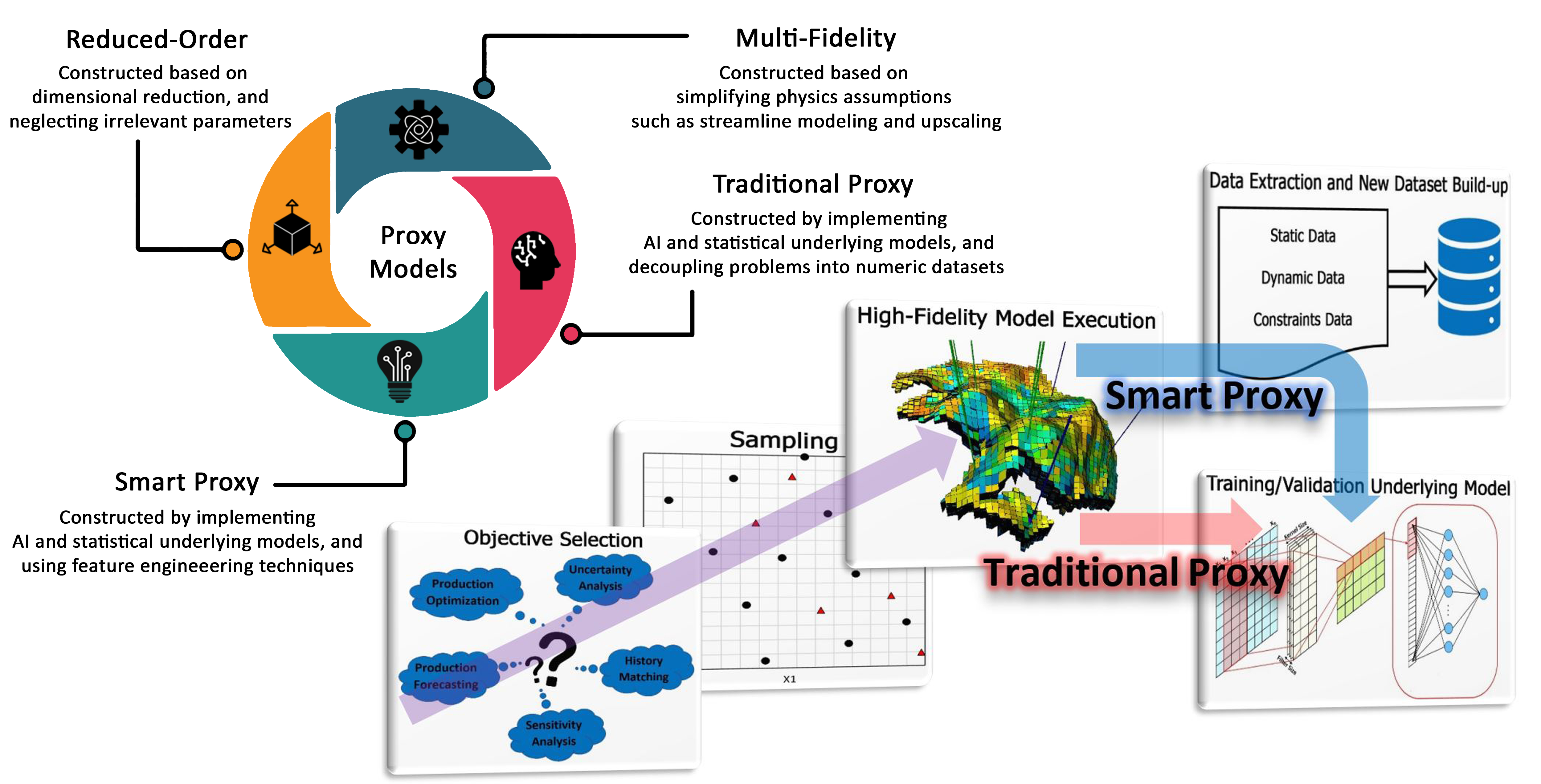
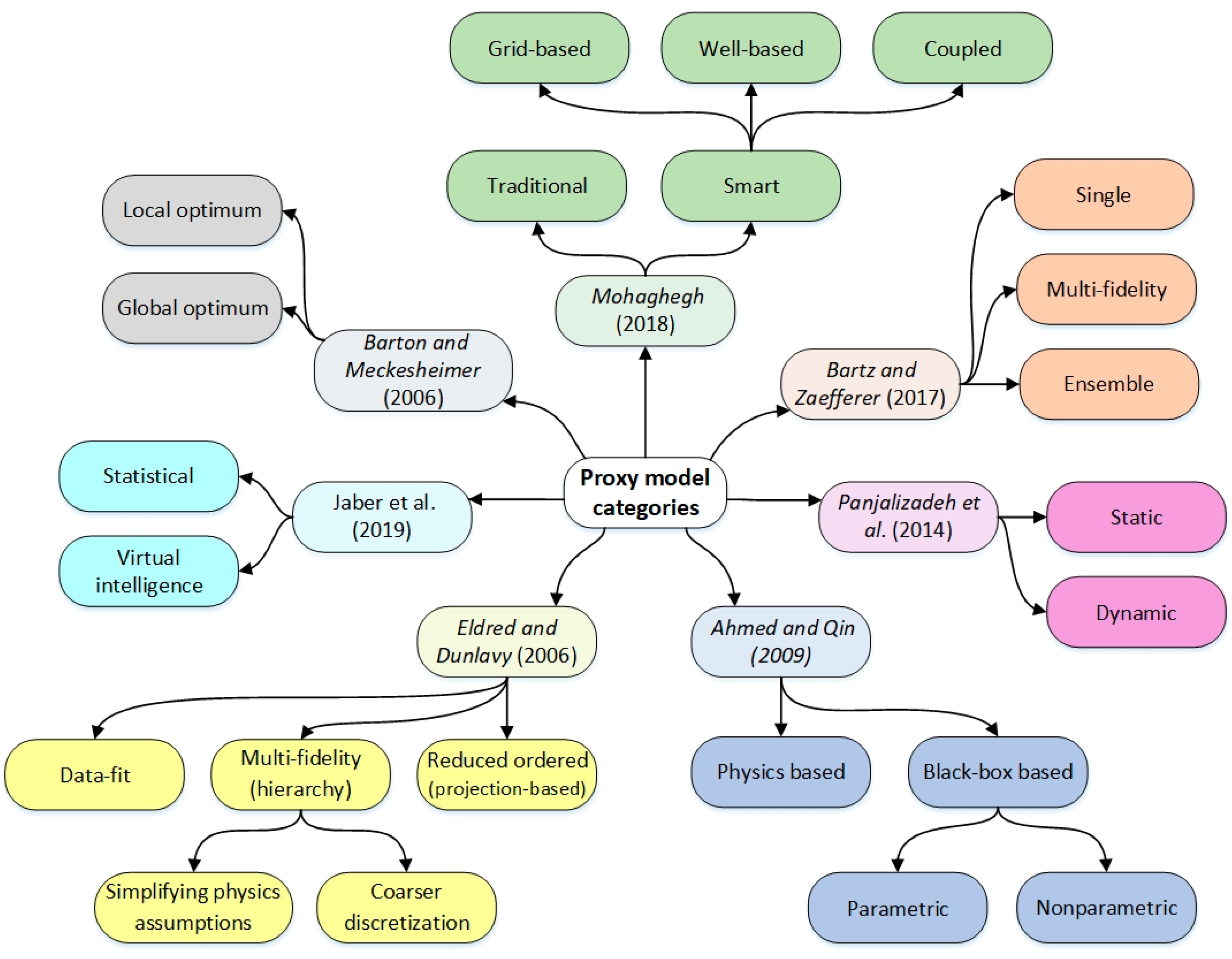
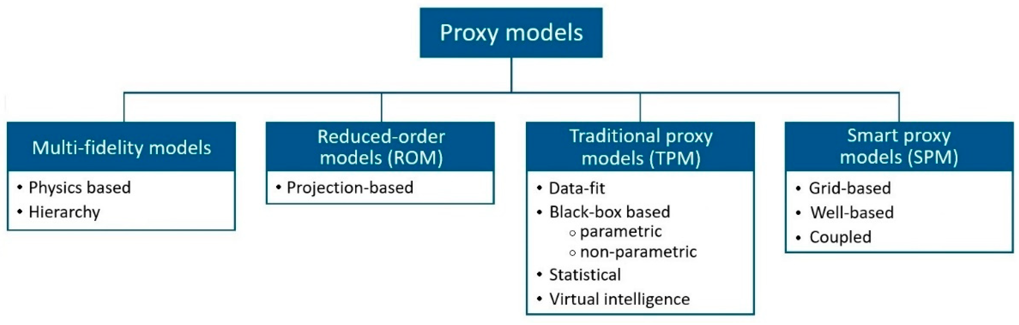
2. Proxy Modeling Classification

PMs can be categorized in various ways, such as by their objective/application, the approximation strategy used, or their time dependency. Figure 2 presents the various ways PMs are classified in the literature.

Ahmed and Qin [8] divided PMs into two groups, black-box-based and physics-based approaches, according to the approximation strategy. In a black-box-based approach, the high-fidelity model cannot be modified, and the PM makes a less expensive approximation of the relationship between inputs and outputs. Conversely, a physics-based approach modifies the governing equations of the problem to make it computationally cheaper, which will be discussed later in this section. Black-box PMs are further divided into parametric and nonparametric, according to the nature of the unknown parameters. In both parametric and nonparametric models, the output parameters are determined using the initial training set; however, parametric models do not implement the training set to make the predictions, whereas nonparametric models do [24]. Polynomial regression (PR) is an example of a parametric model, and kriging (KG), artificial neural networks (ANN), radial basis functions (RBF), multivariate adaptive regression splines (MARS), and support vector regression (SVR) are examples of non-parametric approaches.

Eldred and Dunlavy [9] classified PMs into data-fit, multi-fidelity (also called hierarchy), and reduced-order types (also called projection-based reduced models). Data-fit models, which are primarily used for the evaluation of experimental data, involve the interpolation or regression of the generated results from a few runs of the high-fidelity model. PR, KG, MARS, ANN, and many other methods are examples of data-fit PMs. In data-fit models, the underlying physics does not change, and they are identified as non-physics-based approaches.

A multi-fidelity model, which is a physics-based approach, attempts to solve a low-speed, high-fidelity problem by replacing it with a high-speed, low-fidelity model [24]. Fidelity here is used to describe the level at which a model could reproduce the physics of the desired phenomenon. The process of achieving a lower-fidelity model can be fulfilled through coarser discretization [25], simplifying physics assumptions [26], etc. In an ROM, a high-fidelity model projects down into a low-dimensional system with equivalent characteristics that have fewer degrees of freedom [27]. In other words, an ROM lowers the dimensionality of the primary system by neglecting irrelevant parameters while holding the characteristics and physics over defined space. They are based on the discretization of the underlying partial differential equations of the high-fidelity models. ROMs can be grouped [15] based on the type of system (linear, partially linear or non-linear, parametric or non-parametric, and time-dependent or time-independent). Some popular techniques to solve ROMs are proper orthogonal decompositions (POD) [28], trajectory-piecewise linear (TPWL) [29], and the discrete empirical interpolation method (DEIM) [30], and they are further explained in Section 4.2. In some studies, the terms “multi-fidelity model” and “reduced-order model” have been interchangeably used, and they are considered within one group [16,17]; however, the majority of the literature considers them as separate models.

There are pros and cons to each of the three types of PMs in this classification (data-fit, MFM, and ROM). Data-fit models are easy to use in low-dimensional problems; however, if the number of parameters increases, their application is problematic. Additionally, data-fit models cannot approximate functions other than first- and second-order responses, and the high-fidelity models need to be run many times [31]. To use MFMs, a significant engineering effort is required, and they are usually implemented in an opportunistic manner with the made assumptions. In contrast, the data-fit and reduced-order models are mathematically derived from the high-fidelity model [24]. Although the use of ROMs requires a good understanding of simulation codes for projection, they do not require numerous computational models (that might not always be accessible), in comparison with MFMs [9]. Data-fit models and ROMs can be compared in different aspects. One is that the procedure of generating the PMs using the data-fit models is non-intrusive, and it is only needs to define the system inputs and obtain the outputs by running the high-fidelity model. On the other hand, this procedure is intrusive for ROMs, and system operators should be projected into a reduced subspace [24]. Another feature of ROMs is that they are capable of estimating the errors and bounds between the high-fidelity model and the reduced one [32]. Additionally, ROMs are considered as physics-based models; therefore, they have the advantage of better prediction accuracy compared with the data-fit models, and as they retain the underlying physics, they are even capable of extrapolating away from the initially given space. As a result, they can evolve dynamically in time [9].

Another way to classify PMs is based on time dependency, i.e., static and dynamic modeling [10]. Static PMs are typically built for one or a few discrete time steps and are not valid for processes at other times. In static modeling, only the spatial phenomenon is important. On the contrary, if temporal dependence is added, then the phenomenon is treated as dynamic rather than static, and it is called dynamic or time-dependent proxy modeling. Dynamic models are constructed for the whole desired time interval, not just discrete times [10]. There may be some spatial dependency in the context of static modeling, but no orders in time are effective. In contrast, in temporal or dynamic modeling, past, present, and future concepts exist. In a temporal definition, the sample locations happen in the past, and the predictions extrapolate the future [33]. Some of the popular techniques to deal with spatial problems are described in Section 3.3. To model temporal problems, other techniques, such as a recurrent neural networks, are needed. For details about the models that deal with temporal datasets, please refer to the book written by Lazzeri [34].

Mohaghegh [11] divides PMs into two main categories: traditional and smart. The previously discussed methods (data-fit, MFM, and ROM) fall into the “traditional” proxy model (TPM) category. “Smart” proxy models (SPMs) are trained using machine learning and pattern recognition techniques and require some additional steps in the development process, compared to TPMs. The development steps will be discussed in detail in Section 3. SPMs are capable of reproducing the high-fidelity models without reducing the physics and order of the original system, and they do not decrease the resolution of the model in time or space [35]. SPMs can be developed as grid-based or well-based models depending on the objective of the study [36]. The SPM is referred to as well-based if the objective is to make predictions for parameters at the well locations, such as production rates for oil, gas, and water [37]. In reservoir engineering, production optimization and history matching fall within this class of SPM. If it is desired to build the SPM with outputs at the grid level, it is considered grid-based. Pressure and saturation prediction for different phases are examples of parameters at the grid level, and monitoring their alteration is of paramount importance during injection scenarios where front propagation tracking is needed [38]. Gholami et al. [18] developed another class of SPM; a coupled SPM, which is a combination of well-based and grid-based models and is able to generate the results both in well and grid levels simultaneously. Gholami used a workflow to transfer the parameters between grid-based and well-based models, and she used a cascading procedure to produce the results when the model moves forward in time.

If the objective for generating the proxy model is optimization, it is called surrogate model-based optimization (SBO). Bartz and Zaefferer [12] grouped the SBOs into three types: single, multi-fidelity, and ensemble models. In single SBO, there is only one model to construct the PM in the specified search space. Multi-fidelity and ensemble SBOs use more than one model to approximate the high-fidelity model; however, the multi-fidelity models describe the high-fidelity model in different levels of detail, whereas the ensemble model presents it at the same level of detail. Any of the single, multi-fidelity, or ensemble SBOs can then be coupled with either deterministic or non-deterministic optimization algorithms to optimize the output. Barton and Meckesheimer [13] described SBO in two groups based on the way they search for the optimum. One group updates in an iterative manner and looks for local optimums, and the other finds the global optimum with only one fitting chance. ANN and KG are examples of a global surrogate model, which can be coupled with a non-deterministic (evolutionary) optimization algorithm to find the global optimum. On the other hand, for the local surrogate model, we can name RSM as an example that can be coupled with a deterministic algorithm to find the local optimums [39].

Other classifications for PMs can be seen in the literature; for example, Jaber et al. [14] divide PMs into statistical and virtual intelligence models. The statistical models involve using RSM, and the virtual intelligence models employ machine learning techniques.

We discussed earlier in this section that Mohaghegh considered the PMs in two broad classes of SPMs and TPMs. However, PMs in this work are classified into four classes: MFMs, ROMs, TPMs, and SPMs. Each of these classes has a different development procedure. The development methodology for SPM and TPM will be discussed in Section 3. Figure 3 summarizes the different classes of PMs mentioned under the classification used in this review, and it groups them into four main categories.

3. Methodology

The development of ROMs is based on the projection of the problem into a lower-dimensional case, and MFMs are based on simplifying physics. Detailing the procedure to develop these two proxy types is not the purpose of this work. Instead, it is more focused on the TPMs and SPMs. TPMs in this paper include all classes of PMs that have a development procedure similar to the one shown in Figure 4, such as data-fit, parametric and non-parametric, statistical or virtual intelligence, and static or dynamic. The development strategy of SPM is also presented in Figure 4 based on the strategy introduced by Mohaghegh [11].

A proxy model cannot be built without a high-fidelity model. For example, in the case of reservoir modeling, the high-fidelity model is the numerical simulator. The main steps to construct a TPM include the following: (1) define the objective, inputs, and output parameters for the high-fidelity model with their range, (2) perform the sensitivity analysis if needed, (3) perform the sampling and generation of different design scenarios, (4) run the high-fidelity model to produce the preliminary results, (5) train and validate a new underlying model, and (6) employ a TPM to generate results.

In the first step, which may be considered the most crucial, the reason to construct the TPM is determined. The high-fidelity model (or subsequent TPM) may be used to accomplish many objectives. Optimizing a parameter such as total production rate or watercut in a waterflooding scenario, obtaining the lowest net present value, or history matching are examples of objectives. Then, depending on the objective, the essential parameters with their ranges for the output of the problem must be selected. For example, in the waterflooding case, injection rates, water viscosity, well production rates, etc., can be the effective parameters. A reservoir environment is considered a non-linear and complex problem in which many parameters play a role. Dealing with many parameters in such an environment and running the simulator based on all the parameters is sometimes very costly and time-consuming. In such a case, SA can find the non-influential inputs and reduce the number of them. So, sensitivity analysis is essential in constructing the PM in cases with a high number of inputs, and is performed before the sampling step [40,41], and it can lower the dimensionality of the model [42]. This will be reviewed in Section 3.1. In the sampling step, we design the experiment, we distribute the parameters in their ranges, and the high-fidelity model runs at these designed selections of parameters. Section 3.2 discusses the sampling techniques in more detail. After running the high-fidelity model and recording the desired output, the new machine learning model trains and validates the inputs and outputs. An issue in this step is the significant number of potential modeling techniques, and sometimes it is difficult to determine what technique is suitable for specific applications. A brief description of the different models is presented in Section 3.3. Finally, the built model, which is referred to as the TPM, can predict the output parameter in a much shorter time for the initially selected design parameters. The TPM can then be used for other purposes such as SA, optimization, uncertainty quantification, etc.

The creation of an SPM has a few additional steps compared to the TPM, as shown in Figure 4. The most crucial part of the SPM, like TPMs, is determining the objective for model construction. Then, a set of effective parameters is picked, and sampling is performed within the specified range for the parameters. In the next step, the high-fidelity model is run to generate different realizations of the model. Then, a combination of static and dynamic parameters (including both inputs and outputs) is extracted from the high-fidelity model, and they are used to create a new database [11]. Generating new parameters is called feature engineering, which leads to finding new hidden patterns in the dataset. In TPM construction, we do not involve this step, and the proxy only makes a relationship between the initial design parameters and the output. Hence, SPM provides higher accuracy in approximating the output parameters compared to TPM. Feature engineering also helps SPM to accurately predict the grids’ characteristics. In comparison, TPM suffers in grid-level predictions because a trained model on a limited number of input parameters cannot predict the complex changes in all grids. Neither a TPM nor SPM solves the mathematical equations of a high-fidelity model. They basically decouple the equations, constraints, and complexities of the problem into a numeric dataset. This dataset then can be used to train a(n) AI/statistical model to approximate the desired output. Decoupling the equations makes the TPM and SPM superior to MFM or ROM. It is worth mentioning that the MFM and ROM are the simplified or reduced form of the high-fidelity model, and their construction still needs a great knowledge of the problem. However, TPM and SPM require less scientific knowledge, and they need less time and effort in development.

For a well-based dataset, the rows (observations) in the new dataset are the wells in the reservoir model, and the columns are the extracted parameters from the high-fidelity model at the well level and various time steps. However, for a grid-based dataset, the rows are the individual grids within the high-fidelity model, and the columns are parameters extracted at the grid level and various time steps. For example, Gholami et al. [18] considered various parameters such as porosity, permeability, pressure, saturation for phases, location of the grids, distances to the boundary and closest offset well, production data, bottom-hole pressure (BHP), etc., as the parameters of the grid-based dataset. The authors introduced a tiering system to consider the impact of the surrounding grids as well, and the static and dynamic parameters related to the tiers were imported into the dataset. Such datasets for the generation of the smart proxies would be massive, and reducing both the number of observations and parameters prior to the proxy development would be needed. In the aforementioned work [18], the authors reduced the size of the dataset (from 396,000 to 55,000 observations, and over 1000 parameters to 310 only for one of the realizations out of 13) through grid lumping in the Z-direction and feature selection techniques. The number of parameters in the dataset depends on the number of introduced tiers, offset wells, and the previous timesteps that are going to be cascaded into the new timestep. After forming the dataset, the rest of the steps are similar to those of the TPM.

The main advantage of using an SPM is that it only takes a few seconds to approximate the full reservoir. However, this is only an advantage if the SPM construction time is reasonable. An SPM produces a massive amount of data, which are extracted from different scenarios or realizations of the high-fidelity model. So, picking a small number of sample points is required to avoid generating such a massive dataset and to decrease the construction time [43]. The number of required runs usually depends on the geological properties and operational constraints, and it should cover as much necessary information as possible, depending on the purpose of the study. For instance, in the work carried out by Gholami et al. [18], the total number of realization runs was only 13 for the four design parameters, or in the research by He [19], the number of runs was only three for the two parameters of porosity and permeability in a history-matching process. SPM is a novel approach and expects to provide higher accuracy than TPM. TPM approximates the outputs only based on the initial designing parameters, while SPM creates an approximation by involving many new parameters. The newly introduced parameters usually have positive importance on the outputs [11]. The usage of SPM is more significant in grid-based models where it can predict the outputs at the grid level. A TPM with only a few input parameters lacks the prediction ability for the individual grids in the reservoir. There are only a few SPM examples in the literature, and they almost used the same strategy for development [18,19,20,21,22,23]. We suggest that conducting a sensitivity analysis comparing various techniques for the main steps involved in SPM construction can improve the overall SPM accuracy and development time. For example, only the ANN model for the underlying model construction step, stationary Latin hypercube sampling for the sampling step, or similar tiering systems have been tested for the data extraction step. As a result, it is crucial to know the main techniques for each step. Then, it is important to apply the techniques for future research, and compare them to check how each technique improves the SPM in terms of accuracy and construction time. The next sections provide a comprehensive review of the existing procedure and specific step techniques required in TPM and SPM.

3.1. Sensitivity Analysis (SA)

Sensitivity Analysis (SA) can be used to study how the outputs of a model change due to the variation in the inputs of the specified ranges. The input parameter is called “sensitive” if the variation in its range significantly changes the output. Additionally, a parameter is considered “insensitive” or “robust” if the output does not change a lot [44]. SA establishes the importance of parameters and the inner workings of the models, which can lower the dimensionality of the model [42].

Performing an SA can be significant; for instance, a reservoir model that is representative of a very non-linear environment includes many parameters. As a result, many sample points are required to cover all the search space for the parameters, and running a high-fidelity model for all the designed points is very costly. In such a case, with a large number of parameters for the model, SA is an essential step in generating the TPM, and is performed before the sampling step [40,41]. Consequently, SA can find the non-influential parameters and reduce the number of inputs. SA can sometimes be considered as an objective for constructing a TPM [42,45]. The relationship of inputs with the output in a model could be complex and challenging. In this case, a TPM can be constructed based on all the inputs. This TPM can then be used for SA and run numerous times to find the effect of inputs on the output very quickly.

SA is categorized into local sensitivity analysis (LSA) and global sensitivity analysis (GSA) [46]. In LSA, the inputs are subjected to small perturbations at specific points, and the changes in the output parameter are studied. LSA is also known as the one-at-a-time or univariate method [46,47]. It studies the derivative of output to only one input parameter while keeping the rest of the inputs constant. It cannot investigate the effect of all inputs varying at the same time. LSA is popular for models with a low uncertainty level [48], but it is not suitable for complex reservoir modeling problems. On the other hand, in GSA, the behavior of the output over the entire range of the inputs is studied [46]. Some of the common methods for GSA are based on Monte Carlo (MC) sampling, Sobol, or Morris methods, which are based on probability distributions [49]. MC-based sampling methods allow us to analyze the influence of the parameters, but using them is computationally expensive [50]. The MC-based sampling methods can also be used to find the global optimum of a problem. The Sobol method works based on the variance decomposition theory. It investigates the interaction and contribution of input parameters to the output in a certain number of sample points compared to MC [51]. The Morris method, an extension of LSA, studies multiple points in the parameter range instead of only one [52]. More information on GSA methods can be found in Song et al. [53]. Typically, GSA methods that are based on probability distributions need more runs of the high-fidelity model. As a result, they are computationally more expensive compared to LSA.

3.2. Sampling

Sampling is defined as the process of obtaining data points over the search space of the parameters to be able to construct a PM. The quality and performance of a PM depend strongly on the number of sample points in the specified range of parameters [54]. As discussed earlier, one of the merits of using PMs is to provide a fast and accurate duplicate of the high-fidelity model. Regardless of the underlying model, having a large number of sample points to construct the PMs eventually results in an accurate model; however, the computational cost in the generation of the PMs would be significant. Another effective factor in increasing this cost is the number of implemented parameters in the process of creating the model, which has a direct relationship with the number of sample points as well. High computational cost in the construction of the PMs diminishes their applicability compared with the high-fidelity model. This is known as the curse of dimensionality [8,55]. This cost is usually incurred prior to the implementation of the PM in running the high-fidelity model at sample points and steps in designing the model. The objective in sampling is to acquire the maximum information using the minimum possible number of sample points or the minimum number of high-fidelity model runs. Therefore, the selection of a proper sampling strategy to construct a trustworthy PM is of immense importance. Consequently, once the PM is constructed, hundreds or thousands of runs can be completed in a fraction of a second, which is essential in production optimization and field development planning in the oil and gas field.

Sampling strategies are grouped into the two broad classes of stationary (also known as one-shot, static, priori, domain-based, or model-free strategies) and sequential (also known as model-based, adaptative, or posteriori) sampling. The workflow of both techniques is demonstrated in Figure 5.

In stationary sampling, the sample points are distributed throughout the whole design space based on a pattern [57]. In stationary sampling, after the selection of the design points, the high-fidelity model is evaluated at each of the specified input sets, and the corresponding output is obtained. Consequently, the PM is constructed, and it can be applied for further decisions. The advantages of stationary sampling are ease of deployment and uniform coverage of the domain. However, if the performance of the PM was not approved at any stage, the whole procedure should be performed from the beginning with new and more numerous sample points, which increases the cost of computation. The situation becomes even worse when the problem is highly non-linear and many parameters are involved in the process of constructing the PM, which together increases the number of sample points and makes the modeling inefficient and unreasonable [58]. The stationary sampling methods focus on a uniform fill-up of the domain with sample points, and they usually have a fixed pattern in all of the cases under study. Some famous techniques in this category are factorial designs (full and factorial designs), optimal designs, Latin hypercube sampling (LHS), orthogonal array sampling (OAS), and random sampling such as MC.

In the simplest case of full factorial design, which only considers two levels for each parameter, 2^K sample points are generated, where k is the number of parameters. The sample points are maximized in the distance using the full factorial design; however, the number of sample points increases rapidly when the number of parameters increases [59]. The fractional factorial design, a sub-class of the full factorial design, does not consider some sample points in the full factorial design without losing information, making it viable for higher dimensions [60]. Different designs, such as the Plackett–Burman design (PBD), central composite design (CCD), Box–Behnken design (BBD), and Taguchi, fall into the category of fractional factorial designs [61]. In optimal designs, the parameters are determined without bias and with minimum variance; hence, they require a lower number of sample points [62].

LHS, as a stratified sampling technique, divides each parameter into N bins or equal intervals. Then, each bin for each of the parameters fills with only one sample point. In LHS, there is control over the number of sample points, which is a big advantage in the construction of a PM, where we are looking to limit the number of high-fidelity runs [63]. However, not all Latin hypercube designs uniformly distribute the sample points in the domain, and it is necessary to optimize the space-filling procedure. Viana et al. reviewed some of the techniques to optimize the LHS to better fill up the domain under study [64].

OAS is a generalization of LHS, and it uniformly distributes the sample points in the dimensional projection of the parameter dimensional domain [56,65]. In OAS, four parameters—sample point size, domain dimension, the number of bins per dimension, and the strength—need to be defined. For example, OAS (9, 2, 3, 2) includes nine sample points, two domain dimensions, three bins per dimension, and a strength of two. LHS is considered as an OAS with a strength of one. To understand the construction procedure, and for details about OAS, refer to the work carried out by Hedayat et al. [65]. The selection of the four parameters of OAS is sometimes challenging. Additionally, different selections for bins and the placement of samples in the bins might exist for each problem, limiting OAS usage [58]. In MC, the independent samples are randomly generated, and this process is repeated many times to achieve the desired quantity.

In sequential sampling, the sample size starts with an initial and limited number of points, and new data points are added to the existing ones. The model then stops once it reaches a preferred performance and accuracy [66]. Hence, using this approach, the total time to develop a PM is significantly reduced, as less deployment of the high-fidelity model is needed than when using the stationary sampling technique [67]. There are two main objectives in sequential sampling, known as exploration and exploitation. Exploration means evenly filling up the search space and avoiding redundant new samples. The intention of the exploration part of sequential sampling is the same as stationary sampling, and it tries to find new pivotal regions such as discontinuities and the global optimum. In exploration, the new samples are chosen only based on the initial samples, not the responses of the high-fidelity model [56]. The methods with exploration objectives are usually referred to as exploration-based sequential sampling. Markov chain Monte Carlo (MCMC), low-discrepancy sequence methods (such as Sobol and Halton), nested LHS, and quasi LHS are examples of this subcategory.

MCMC is based on a sequence of random sampling from a probability distribution. In MCMC, the sample points are generated systematically in such a way that the new sample point is probabilistically dependent on the prior sample point [68]. In the low-discrepancy sequences, the term “low-discrepancy” implies that the sample points are, more or less, equally spread within the domain of parameters. A low-discrepancy sequence is a sequence with the property that all the new points are as far as possible from the existing points. In Sobol and Halton sequences [69,70], the sample points are randomly produced within the parameters’ domain without overlapping the existing points in a progressive manner. However, Sobol outperforms Halton as the number of dimensions increases [71]. We can use nested and quasi-LHS to sequentially generate the sample points for LHS. Nested LHS includes various designs requiring one as the subset of another one [72]. The evaluation performs on the smallest subset, and if the results are not desirable, the superset could be evaluated. This process can continue to the next supersets. Here, each subset is known as a layer, which is an LHS with a level of accuracy [73]. In quasi-LHS, the new sample points are added to keep the distance from the existing design points [74].

Exploitation-based sampling techniques look for regions that have already been recognized as key domains and add the new sample points at each iteration focused on these regions. In exploitation, unlike exploration, the new samples are added only based on the information provided by the high-fidelity model. The LOLA-Voronoi sampling method [56] falls into this subcategory. This method works based on the local gradient approximation to find the non-linearity of the problem under study, and it picks more sample points near the non-linear region to increase the chance to find the local optimum.

3.3. Popular Models for PM Construction

PMs, as discussed in Section 2, can fall into different categories. This section discusses the most prominent underlying models that can be used in the construction of TPMs or SPMs.

3.3.1. Polynomial Regression (PR)

PR is the most straightforward technique to construct a PM. It fits a non-linear relationship at any order between the inputs (x_i) and the output (y). PR is also known for the response surface method. It is usually applicable for lower-dimensional problems and is not suitable for high-dimensional and highly non-linear systems. PR can be given by the general form of Equation (1).

$$\begin{array}{ll}\hat{\mathrm{y}}\left({\mathrm{x}}_1, {\mathrm{x}}_1, \dots , {\mathrm{x}}_{\mathrm{m}}\right)& +{\displaystyle {\displaystyle \sum }_{{\mathrm{s}}_1=1}^{\mathrm{m}}}{\mathsf{\beta }}_{{\mathrm{s}}_1}({\mathrm{x}}_{{\mathrm{s}}_1})+{\displaystyle {\displaystyle \sum }_{{\mathrm{s}}_1=1}^{\mathrm{m}}{\displaystyle \sum }_{{\mathrm{s}}_2={\mathrm{s}}_1}^{\mathrm{m}}}{\mathsf{\beta }}_{{\mathrm{s}}_1{\mathrm{s}}_2}({\mathrm{x}}_{{\mathrm{s}}_1}{\mathrm{x}}_{{\mathrm{s}}_2})+\dots \\ & +{\displaystyle {\displaystyle \sum }_{{\mathrm{s}}_1=1}^{\mathrm{m}}{\displaystyle \sum }_{{\mathrm{s}}_2={\mathrm{s}}_1}^{\mathrm{m}}}\dots {\displaystyle {\displaystyle \sum }_{{\mathrm{s}}_{\mathrm{p}}={\mathrm{s}}_{\mathrm{p}-1}}^{\mathrm{m}}}{\mathsf{\beta }}_{{\mathrm{s}}_1{\mathrm{s}}_2\dots {\mathrm{s}}_{\mathrm{p}}}({\mathrm{x}}_{{\mathrm{s}}_1}{\mathrm{x}}_{{\mathrm{s}}_2}\dots )\end{array}$$

(1)

where ŷ is the approximated output, m is the number of dimensions or parameters, β is the polynomial coefficient, and p is the polynomial order. To construct a high-order polynomial, a large number of training points are needed. Furthermore, high-order PR models cause instability and sometimes yield a false optimum [75].

3.3.2. Kriging (KG)

KG or Gaussian process regression is a technique to interpolate the output based on the Gaussian process by considering the prior covariances [76]. In 1989, Sacks et al. [77] used the KG to construct a PM for the first time in engineering. There is always a residual error ε between a PM response (ŷ) and the high-fidelity model response (y).

$$\mathrm{y}\left(\mathrm{x}\right)=\hat{\mathrm{y}}\left(\mathrm{x}\right)+\mathsf{\epsilon }$$

(2)

The basic assumption behind most PMs is that this residual error between the responses of models is independent. However, in KG models, this error is dependent on another term [78]. KG involves using a polynomial function f(x) and a random function (i.e., stochastic process) Z(x).

$$\mathrm{y}\left(\mathrm{x}\right)=\mathrm{f}\left(\mathrm{x}\right)+\mathrm{Z}\left(\mathrm{x}\right)$$

(3)

The polynomial term determines the global trend of the data, and the stochastic term accounts for the deviation of the output from the polynomial term. The stochastic term Z(x) is assumed to have zero mean and variance of σ². In many problems, the polynomial term f(x) can be replaced by a constant without losing performance, and this is known as Ordinary KG [79].

A KG proxy model is suitable for low-order non-linear and large-scale problems, and it can work for a wide range of sample sizes and designs. However, applying it to a large-scale problem might be time-consuming [80]. It also does not work accurately for problems containing discontinued parameters and a dimensionality higher than 20 [81].

3.3.3. Multivariate Adaptive Regression Splines (MARS)

MARS, introduced by Friedman [82], is a regression algorithm that implements linear regression modeling for the sub-intervals of each design parameter. The location at which the sub-intervals connect to each other is known as a knot. MARS is an extension of linear regression models, and it uses a set of coefficients and basis functions to make a relationship between inputs and the output. The process of constructing MARS happens in forward/backward iterations for different sub-intervals. First, it creates a basis function (i.e., spline) for each sub-interval with its corresponding linear regression and coefficients. In the forward procedure, it looks for the optimum locations to place the knots.

$$\hat{\mathrm{y}}\left(\mathrm{x}, \mathsf{\beta }\right)={\displaystyle \sum }_{\mathrm{m}=1}^{\mathrm{M}}{\mathsf{\beta }}_{\mathrm{m}}{\mathrm{B}}_{\mathrm{m}}\left(\mathrm{x}\right)$$

(4)

where β_m is a vector of regression coefficients, M is the number of basis functions, and B_m is the basis function which can be described as

$${\mathrm{B}}_{\mathrm{m}}\left(\mathrm{x}\right)={\displaystyle \prod }_{\mathrm{i}=1}^{{\mathrm{k}}_{\mathrm{m}}}{\mathrm{b}}_{\mathrm{i},\mathrm{m}}({\mathrm{x}}_{\mathrm{v}\left(\mathrm{i},\mathrm{m}\right)}-{\mathrm{t}}_{\mathrm{i},\mathrm{m}}{)}_{+}^{\mathrm{q}}$$

(5)

where k_m is the number of design parameters in the mth basis function, b_i,m = ±1, v(i,m) is for labeling the design parameters, x_v(i,m) is the ith parameter in the total of k parameters, t_i,m is the knot location of the corresponding parameter, q is the order of the spline, and + subscript is for the positive part of the function (it is zero for negative values of the function).

$$({\mathrm{x}}_{\mathrm{v}\left(\mathrm{i},\mathrm{m}\right)}-{\mathrm{t}}_{\mathrm{i},\mathrm{m}}{)}_{+}^{\mathrm{q}}=\{\begin{array}{lll}({\mathrm{x}}_{\mathrm{v}\left(\mathrm{i},\mathrm{m}\right)}-{\mathrm{t}}_{\mathrm{i},\mathrm{m}}{)}^{\mathrm{q}}& \mathrm{if}& \left({\mathrm{x}}_{\mathrm{v}\left(\mathrm{i},\mathrm{m}\right)}-{\mathrm{t}}_{\mathrm{i},\mathrm{m}}\right)>0\\ 0& \mathrm{if}& \left({\mathrm{x}}_{\mathrm{v}\left(\mathrm{i},\mathrm{m}\right)}-{\mathrm{t}}_{\mathrm{i},\mathrm{m}}\right)\le 0\end{array}$$

(6)

In the forward step, the algorithm creates functions and looks for the locations of the knots to improve the performance, which might cause overfitting. In the backward step, MARS prunes the non-influential design parameters based on the generalized cross-validation techniques [83].

MARS is suitable to deal with large and high-dimensional datasets. It is capable of performing feature selection through the backward step; however, choosing the knot locations is challenging, and it sometimes faces overfitting [84].

3.3.4. Artificial Neural Networks (ANN)

ANN works based on the biological neural system in the brain, which consists of many chemically connected neurons [85]. Neurons are placed in three main layers: input, hidden, and output layers. Neurons receive signals from neurons in the previous layer and transmit them to the next layer. Each neuron is accompanied by a weighting factor that should be adjusted. Adjusting the weights usually happens via an optimization algorithm, most often via the backpropagation technique [81]. The receiving signal for a neuron in the hidden layer multiplies into the adjusted weights and sum. Then, an activation function is applied to the summation to generate the output for that neuron. Some commonly used activation functions are linear, sigmoid, rectified linear unit (ReLU), and hyperbolic tangent [86]. There are some controlling parameters that should be optimized to have an accurate ANN model, such as the number of hidden layers, the number of neurons in each layer, and the activation function. ANN can approximate the problems with unknown nature, but sometimes finding the optimal controlling parameters is challenging. Additionally, using the ANN is computationally expensive, and it requires high memory. Recurrent neural networks (RNN) and convolutional neural networks (CNN) are two well-known and robust types of ANN. RNN works similarly to backpropagation ANN, with the difference that RNN has a memory to store information, and is suitable for a sequence of data and time-series data [87], whereas CNN adaptively learns spatial patterns within the parameters, and is designed to process data in grid formats such as images [88].

3.3.5. Radial Basis Function (RBF)

RBF is a network that includes an input layer of nodes, a hidden layer with a radial basis function (kernel), and an output layer of linear weights [89]. This network approximates the problem in a feed-forward process through Equation (7).

$$\hat{\mathrm{y}}\left({\mathrm{x}}_{\mathrm{p}}\right)={\displaystyle \sum }_{\mathrm{i}=1}^{\mathrm{N}}{\mathrm{w}}_{\mathrm{i}}{\mathsf{\varphi }}_{\mathrm{i}}\left({\mathrm{x}}_{\mathrm{i}},{\mathrm{x}}_{\mathrm{p}}\right)$$

(7)

where x_p is the vector of inputs, x_i is the ith center of the total N radial functions, ϕ_i(x_i, x_p) is the ith kernel to calculate the distance between x_i and x_p, and w_i is the corresponding weight factor for the radial function. The radial function can be selected in different forms such as linear, cubic, thin plate spline, Gaussian, multi-quadratic, and inverse multi-quadratic. Several methods exist to define the centers of the radial functions, such as the orthogonal least-squares method [90].

RBF, like ANN, is easy to implement; however, RBF is suitable for training noisy datasets because of its non-linear characteristics. RBF is not recommended for problems with a high number of parameters that would be very expensive to compute.

3.3.6. Support Vector Regression (SVR)

SVR was first developed by Vapnik [91] to find a function to relate the inputs and the output. It can approximate the problem based on the weighted sum of basis functions added to a constant term as

$$\hat{\mathrm{y}}\left(\mathrm{x}\right)=\mathsf{\mu }+{\displaystyle \sum }_{\mathrm{i}=1}^{\mathrm{n}}{\mathrm{w}}_{\mathrm{i}}{\mathsf{\varphi }}_{\mathrm{i}}\left({\mathrm{x}}_{\mathrm{i}},\mathrm{x}\right)$$

(8)

where μ is a constant bias term, ϕ is the basis function, and w_i is the corresponding weight factor for the basis function. For the basis function, either linear or non-linear functions can be considered. The main idea behind the SVM is to look for the best fit line (hyperplane) and the boundary lines to obtain the maximum number of data points. The formula used to approximate the output in SVR is similar to RBF; however, the methods they use to obtain the unknowns are different. In RBF, the unknowns are determined by minimizing the error between the actual and predicted outputs, but in SVR, μ and w are obtained through solving an optimization problem for the threshold between the hyperplane and the boundary lines [92].

SVR has the advantage of accurate and fast prediction, and it is robust to outliers. Furthermore, SVR is suitable for high-dimensional problems with non-linear data. However, training SVM and selecting the appropriate parameters is challenging [93].

3.3.7. Genetic Programming (GP)

GP was initially proposed by Koza [94], which is an extension of the genetic algorithm (GA), and it is used mostly for symbolic regression. Both techniques are based on evolutionary Darwinian theory. They start with a population of random solutions (known as parents), and the solutions evolve through generations by dropping the not-fitted solutions. In GA, these candidates are in the form of coded strings (also known as chromosomes), while they are in the form of mathematical expressions in GP [95]. GP uses a tree structure to represent the mathematical expressions. The two main components of these trees are the function set (nodes) and terminal set (leaves) [94]. The function set can be chosen through mathematical operators, functions, or conditional statements, and the terminal set includes constants and problem parameters. In GP, the evolution mainly happens in two different processes, mutation and crossover. Mutation involves substituting a random new segment with a segment in the parent, and crossover happens by exchanging segments between two parents and forming two new solutions (offspring). The algorithm also reproduces random solutions to compensate for the dropped solutions in the previous generation. All the solutions again check for the fitness in the new generation, and this process continues until an acceptable fitness value is achieved or the algorithm reaches its generation limit.

One of the drawbacks of using GP is that it needs to be run multiple times because of the stochastic nature of the algorithm. The fixed value of the algorithm parameters (such as crossover and mutation probability) constructs different models at each run. Too-simple models may result in poor predictions, and too-complex models may cause overfitting [96]. On the other hand, GP can generate a high number of potential solutions without considering the underlying assumptions of the problems.

3.3.8. Random Forest (RF)

RF is an ensemble learning technique initially developed by Breiman [97]. RF is an ensemble of multiple unpruned decision trees. It implements the bootstrap sampling (bagging) technique, which uses a random selection of the dataset as the training set and uses the rest of the dataset as the testing set for each tree in the ensemble. The random selection in RF helps the diversity in the ensemble of trees and improves the predictions, and prevents overfitting [98]. RF gives the final result as an average of the results from individual trees, also known as aggregation.

In the process of growing individual trees, a small subset of size m out of M parameters for each node (m < M) will randomly be picked to train the trees. The size of m is kept constant during the forest growing, but the parameters are changed for each node. This process helps the model to use all the potential parameters for the prediction and prevents the model from relying on any specific parameters. Consequently, the best split at each node is chosen among m parameters rather than all the parameters of M. Hence, RF involves using the feature selection technique. It analyses all the parameters without deleting them and selects the influential ones [99]. As a result, RF is a suitable algorithm for large datasets with a high number of parameters, and it produces very accurate results even when a part of the data is missed. However, it lacks prediction ability beyond the training data range [100].

3.3.9. Extreme Gradient Boosting (XGboost)

XGboost is a supervised learning method proposed by Chen and Guestrin in 2016 [101], which is based on the gradient boosting machine (GBM) technique introduced by Friedman [102]. In the GBM technique, the algorithm sequentially adds the input parameters to an ensemble of decision trees to help to improve the prediction. Unlike the RF, which is an ensemble of deep independent decision trees, GBM is an ensemble of shallow trees. GBM builds only one decision tree at a time, and it sequentially improves the ensemble’s performance as it goes forward to the next tree [103]. RF involves averaging the results from all the independent decision trees, while GBM calculates the loss function for each tree. XGboost differs from GBM in the way it minimizes the loss function. XGboost uses the second-order gradient of the loss function, which helps to more easily minimize the function. Additionally, the parallel computing ability and the implementation of some generalization terms to prevent overfitting are other benefits to using the XGboost compared to the GBM [104]. Some of the main disadvantages of XGboost are the high training time for large datasets and the inability to predict beyond the training data range.

3.3.10. Polynomial Chaos Expansion (PCE)

PCE was introduced first by Wiener [105] to project the output on an orthogonal stochastic polynomial basis function in the random inputs. The general form of the PCE can be defined as Equation (9) [106]:

$$\hat{\mathrm{y}}\left(\mathrm{X}\right)={\displaystyle \sum }_{\mathsf{\alpha }\in {\mathbb{N}}^{\mathrm{M}}}{\mathsf{\beta }}_{\mathsf{\alpha }}{\mathsf{\Psi }}_{\mathsf{\alpha }}\left(\mathrm{X}\right)$$

(9)

where α is the index with M dimensions, β_α are the deterministic polynomial chaos coefficients, Ψ_α = {Ψ₁, Ψ₂, …, Ψ_M} is a set of multivariate orthogonal polynomial basis, and X is the vector of input parameters with M dimension. The multivariate orthogonal polynomial basis can be written as the product of univariate polynomials ${\mathsf{\varphi }}_{{\mathsf{\alpha }}_{\mathrm{k}}}$ of degree α_k:

$${\mathsf{\Psi }}_{\mathsf{\alpha }}(\mathrm{X})=\prod _{\mathrm{k}=1}^{\mathrm{M}}{\mathsf{\varphi }}_{{\mathsf{\alpha }}_{\mathrm{k}}}(\mathrm{X})$$

(10)

where ${\mathsf{\varphi }}_{{\mathsf{\alpha }}_{\mathrm{k}}}$ is the univariate orthogonal polynomial in the kth parameter of degree α_k. There are different univariate polynomial families such as Hermite (based on Gaussian distribution), Laguerre (based on gamma distribution), and Jacobi (based on beta distribution) [107].

The main benefit of using PCE is that as the order of expansion increases, it guarantees the convergence of ŷ to y, preventing the drawback of overfitting in many other techniques. Additionally, PCE is almost applicable to all input distribution types [108]. However, PCE sometimes slowly converges, and if the order of expansion increases in high-dimensional problems, it requires a large number of high-fidelity model runs. A summary of the aforementioned modeling techniques with their pros and cons is presented in

Table 1. Advantages and disadvantages of different modeling techniques.

Modeling Technique	Advantages	Disadvantages
PR	Suitable for lower-dimensional problems.	Not suitable for high-dimensional and highly non-linear systems. A large number of training points is needed to construct a high-order polynomial [75]. High-order PR models cause instability and sometimes yield a false optimum [75].
KG	Suitable for low-order non-linear and large-scale problems. Works for a wide range of sample sizes and designs.	Applying it to a large-scale problem might be time-consuming [80]. Not accurate for problems containing discontinued parameters and dimensionality higher than 20 [81].
MARS	Suitable to deal with large and high-dimensional datasets. Capable of performing feature selection through the backward step.	Choosing the knot locations is challenging, and it sometimes faces overfitting [84].
ANN	It can approximate problems with unknown nature. Easy implementation.	Finding the optimal controlling parameters is challenging. It is computationally expensive, and it requires high memory.
RBF	Suitable for noisy datasets. Easy implementation.	Very expensive computation for problems with a high number of parameters.
SVR	It is accurate with fast prediction. It is robust to outliers. Suitable for high-dimensional problems with non-linear data.	Training and selecting the appropriate parameters is challenging [93].
GP	Can generate a high number of potential solutions without considering the underlying assumptions of the problems.	Needs to be run multiple times because of the stochastic nature of the algorithm. Too-simple models may result in poor predictions. Too-complex models may cause overfitting [96].
RF	Suitable for large datasets with a high number of parameters. It produces very accurate results even when a part of the data is missed.	Lacks prediction ability beyond the training data range [100].
XGBoost	Able to perform parallel computing. Implementation of some generalization terms to prevent overfitting.	High training time for large datasets. Unable to predict beyond the training data range.
PCE	Almost applicable to all input distribution types. As the order of expansion increases, it guarantees the convergence of prediction, and prevents overfitting.	It slowly converges. If the order of expansion increases in high-dimensional problems, it requires a large number of high-fidelity model runs.

.

3.4. Optimization

Once the PM with the chosen underlying model is built and evaluated for its accuracy and fitness, the model is ready for further use, such as in predictions and optimization. In the optimization process, to find the best selection of the design parameters, an objective function based on the purpose of the problem should be defined.

Optimizers are divided into deterministic (gradient-based) and stochastic (meta-heuristic) approaches. Deterministic methods implement the gradient of the objective function, and they are suitable for objective functions with a smooth surface. The biggest drawback of deterministic approaches is that their performance depends on the initial guess of the design parameters, and they may become trapped in a local optimum, preventing them from finding the global optimum. Deterministic methods can be categorized into ensemble-based, simultaneous perturbation, and adjoint methods [109].

Stochastic approaches solve the problem by borrowing rules from nature. Popular methods in this category are GA, particle swarm optimization (PSO), simulating annealing, ant colony optimization (ACO), and differential evolution (DE), which are the standard methods to find the global optimum.

GA is an evolutionary algorithm proposed by Holland [110], and it uses Darwin’s rule and creates solutions by implementing processes such as mutation and crossover, which was previously discussed in Section 3.3.7. GA is a strong method to find the global optimum that works for both continuous and discrete optimization problems. GA can be parallelized and is applicable to multi-objective functions in global optimization problems [101]; however, it is computationally expensive and time-consuming [111].

PSO, like GA, is a population-based method, and it uses the collective behavior of animal groups such as birds and fish. PSO was first introduced by Kennedy and Eberhart [112]. The algorithm generates random solutions in which each solution is known as a particle, and the group of particles forms a swarm. Each particle in the swarm moves in the searching space of the design parameters. The position and velocity of the particles continue to update at each step based on the individual and global best solutions at the previous step until the particles find the global optimum. PSO has less computational burden but is more reliable in finding the global optimum compared to GA. Furthermore, the PSO approach is less effective for problems of more than three input parameters [111].

Simulating annealing is a probabilistic method that is inspired by the annealing process in metals [113]. Simulating annealing allows finding the global optimum in a large search space with the ability to jump out of any local optimum it finds [114]. In the simulating annealing algorithm, the controlling parameter is called temperature. The algorithm starts with a positive temperature, and this temperature decreases gradually to a zero value. At each step, a random solution close to the previous solution is generated, and it tries to move the temperature-dependent probability toward zero. In other words, while the algorithm searches the working space, the probability of accepting worse solutions gradually decreases. Simulating annealing is suitable for problems that contain many local optimums, and it also works on problems with discrete search space [115].

ACO is also a population-based algorithm and works based on the behavior of real ants when they are searching for food [116]. Real ants find the shortest path between a food source and the colony by communicating with each other and following substances named pheromones. If they sense a pheromone in their vicinity, they reinforce their movement toward that path. Similarly, in optimization problems, artificial ants iteratively search the domain space of parameters for the best solution in different generations. When an ant finds a solution, it marks the path to that solution as a transition rule and deposits an amount of pheromone on that route. The fitness of that path or the solution is determined based on the amount of pheromone left on that path. In the next generations, the ants are guided by the pheromone concentration left by the previous generations toward better solutions. ACO shows similar advantages and disadvantages to PSO, and it is not suitable for problems with more than three dimensions [111].

DE, as a population-based algorithm, was first proposed by Price et al. [117] for global optimization over continuous search space. Despite its name, this method does not require any calculations for the gradient, and the problem does not need to be differentiable. DE is a robust technique that converges to the solution, requiring only a few controlling parameters. The algorithm starts searching the design space by creating a population of random solutions and forms new solutions by combining the existing ones. DE, like GA, involves using mutation, crossover, and selection, which help the solutions evolve at each generation. However, DE deals differently with mutation and crossover. DE performs the mutation by creating a mutant vector of three randomly selected vectors and performs the crossover by creating a trial vector of the mutant vector and target vector [118]. Then, the fitness of the trial and target vectors is evaluated, and the best is kept for the next generation [119]. In DE, the selection of the parent solution is not based on fitness. In contrast, every solution is selected as a target vector (one of the parents); therefore, all the vectors have the chance to be one of the parents. DE only needs to adjust three parameters, and it has lower computational complexity compared to GA. Additionally, the algorithm stops the solution from being trapped in local optimums [120]. Nevertheless, adjusting the controlling parameters is sometimes challenging [121].

4. Application of Proxy Models in the Oil and Gas Industry

This section discusses the application of different proxy types in the oil and gas industry, especially in reservoir modeling. Based on the literature, data-fit models are prevalent, and the application of MFMs and ROMs is limited. This review tries to cover the comprehensive implementation of all types of proxy models in different areas of the subsurface environment. Various applications of proxy modeling such as SA, uncertainty quantification, risk analysis, history matching, field development planning, and reservoir characterization are presented in this section. Furthermore, implemented cases for other models are briefly discussed in this section.

4.1. Multi-Fidelity Models (MFM)

MFMs try to reduce the physics of the problem. Streamline modeling, upscaling, and capacitance-resistance modeling (CRM) are the most popular techniques of MFMs in reservoir modeling. Streamline models decouple the governing flow equations in a reservoir along one-dimensional streamlines, and as a result, they boost the speed of calculation [122]. Streamline modeling has been applied in a variety of subsurface problems, such as production optimization, mainly through waterflooding [123,124], uncertainty quantification [125], history matching [126,127,128,129], and well placement optimization [130]. Streamline models are often applied to a fine-scale reservoir model [131], and they need to run the high-fidelity model at different time steps. Consequently, the speedup capability of streamline models is limited [132]. In upscaling, as another way to simplify the physics, the equivalent petrophysical properties at a coarser scale are calculated [133]. Upscaling has been implemented for a wide range of objectives in reservoir modeling [134,135,136,137].

The idea of duplicating the subsurface behavior using a circuit of capacitors and resistors was first presented by Bruce in 1943 [138]. He used this concept to mimic the behavior of a strong water drive reservoir. This was achieved by comparing the governing equations of electrical circuits and porous media; the potential difference is the motive for the electrons to flow in electrical circuits while the pressure difference is the main reason for the fluid flow in porous media. Both systems have the characteristic of storing energy. In subsurface porous media, compressibility causes the fluid to accumulate, but the electrons are stored in capacitors. CRM was first presented by Yousef et al. [139]. The proposed model was capable of mimicking the porous media behavior between injectors and producers to identify the transmissibility trends and flow barriers. CRM estimates the values for parameters by relating the input and output signals. It considers the pressure changes caused by injectors and the aquifer as the inputs, production rates as the outputs, and the properties of rock and fluid (such as compressibility and saturation) as the related parameters. The CRMs can provide an insight into the interwell connectivity, drainage volume, and reservoir heterogeneity, for example, by channeling along the layers [140]. Furthermore, they can be applied for history matching and production forecasting, requiring only production/injection rates and BHPs [141,142].

In general, any technique that tries to solve the problem by simplifying the underlying physics is an example of an MFM. For example, in work carried out by Wilson and Durlofsky [143], in which a dual-porosity, dual-permeability reservoir model was simplified into a single-porosity, single-permeability model, the model can be considered as a reduced physics or a MFM proxy approach.

4.2. Reduced-Order Models (ROM)

The popular methods in the class of ROM that are used for reservoir modeling approximations are POD, TPWL, and DEIM. As discussed in Section 2, ROM methods project the exact model into a lower-dimensional subspace. The subspace basis in POD is achieved by accomplishing a singular value decomposition of a matrix containing the solution states obtained from previous runs [144]. POD has been implemented in different areas such as reservoir modeling [145,146], finding the optimal control parameters in water flooding [147,148], and history matching [149]. Nevertheless, POD methods need to solve the full Jacobean of the matrix for projecting the non-linear terms in every iteration. Since the reservoir environment is highly non-linear, the speedup potential of POD to approximate the reservoir simulation is not significant. For instance, Cardoso et al. [146] achieved speedups of at most a factor of 10 for ROMs based on POD in reservoir simulation. To solve this drawback, retain the non-linear feature of parameters and further increase the speedup potential, a combination of the TPWL or DEIM method and POD has been the focus of attention in the literature. The combination of TPWL and POD was implanted in various cases such as waterflooding optimization [150,151], history matching [152,153], thermal recovery process [154], reservoir simulation [150], and compositional simulation [155]. In work carried out by Cardoso and Durlofsky [150], a POD in combination with TPWL could increase the speedup for the same reservoir discussed earlier from a factor of 10 to 450. Additionally, the application of DEIM and POD is applied in some studies to create proxies for reservoir simulation [156,157], fluid flow in porous media [158,159], and water flooding optimization [160].

Other methods to treat the non-linearity can be pointed out, such as Gauss–Newton with approximated tensors [161], truncated balanced realization [160], localized discrete empirical interpolation method [162], trajectory piecewise quadratic [163], and sparse proper orthogonal decomposition—Galerkin [164]. A comprehensive study of these methods in reservoir modeling can be found in work carried out by Suwartadi [165] and He [166].

4.3. Traditional Proxy Models (TPM)

In the literature, a wide variety of techniques can be considered as TPMs. This type of proxy can approximate different areas in the subsurface or surface environment such as production optimization [100,167], uncertainty quantification [168,169], history matching [170,171], field development planning [172], risk analysis [173,174], gas lift optimization [109,175], gas storage management [176], screening purposes in fractured reservoirs [177], hydraulic fracturing [178], assessing the petrophysical and geomechanical properties of shale reservoirs [179], waterflooding optimization [180,181,182,183], well placement optimization [184,185,186], wellhead data interpretation [187], and well control optimization [188]. Additionally, TPMs have a wide range of applications in various EOR recovery techniques such as steam-assisted gravity drainage (SAGD) [189], CO₂-gas-assisted gravity drainage (GAGD) [190], water alternating gas (WAG) [191,192], and chemical flooding [193].

4.4. Smart Proxy Models (SPM)

SPMs are implemented in various areas such as waterflood monitoring [20,194], gas injection monitoring [21], and WAG monitoring [18] using the grid-based SPM, history matching [19,22], and production optimization in a WAG process [18] using the well-based SPM. A brief summary of the PMs (including the TPMs and SPMs) used in the literature can be found in Table 2.

Table 2. Examples of PM applications in reservoir modeling.

Ref.	Subject	Sampling Technique	Underlying Model	Optimizer	Class
Kovscek and Wang [125]	Uncertainty quantification in a carbon dioxide storage case	-	Streamlines	-	MFM
Tanaka et al. [123]	Production optimization in waterflooding	-	Streamlines	GA	MFM
Wang and Kovscek [126]	History matching in a heterogeneous reservoir	-	Streamlines	-	MFM
Tang et al. [195]	Investigating the effects of the permeability heterogeneity and well completion in near-wellbore region	-	Streamlines	-	MFM
Kam et al. [128]	Three-phase history matching	-	Streamlines	GA	MFM
Taware et al. [130]	Well placement optimization in a mature carbonate field	-	Streamlines	-	MFM
Allam et al. [134]	History matching	-	Upscaling	-	MFM
Yang et al. [136]	Multiphase uncertainty quantification and history matching	-	Upscaling	-	MFM
Holanda et al. [141]	Reservoir characterization and history matching	-	CRM	-	MFM
Artun [142]	Characterizing interwell reservoir connectivity	-	CRM	-	MFM
Cardoso and Durlofsky [150]	Production optimization in waterflooding	-	TPWL/POD	Gradient-based	ROM
Xiao et al. [152]	History matching	Smolyak sparse [196]	TPWL/POD	Gradient-based	ROM
Rousset et al. [154]	Production prediction of SAGD operation	-	TPWL/POD	-	ROM
He and Durlofsky [155]	Compositional simulation of the reservoir	-	TPWL/POD	-	ROM
Gildin et al. [156]	Simulation of flow in heterogeneous porous media	-	DEIM/POD	-	ROM
Li et al. [158]	Compressible gas flow in porous media	-	DEIM/POD	-	ROM
Alghareeb and Williams [160]	Production optimization in waterflooding	-	DEIM/POD	-	ROM
Al-Mudhafar [100]	Production optimization in cyclic CO2 flooding	-	PR, MARS, RF	-	TPM
Golzari et al. [167]	Production optimization in three different cases to increase recovery and net present value (NPV)	Adaptive LHS	ANN	GA	TPM
Amiri Kolajoobi et al. [168]	Uncertainty quantification and determination of cumulative oil production	LHS	ANN	-	TPM
Peng and Gupta [169]	Uncertainty quantification in a fluvial reservoir	Factorial	PR	-	TPM
Zubarev [170]	History matching and production optimization	LHS	PR, KG, ANN	GA	TPM
Guo et al. [171]	History matching in a channelized reservoir	Random selection	SVR	Distributed Gauss–Newton [197]	TPM
Avansi [172]	Field development planning	BBD	PR	-	TPM
Ligero et al. [173]	Risk assessment in economic and technical parameters on an offshore field	Factorial	PR	-	TPM
Risso et al. [174]	Assessment of risk curves for uncertainties in the reservoir	BBD, CCD	PR	-	TPM
Ghassemzadeh and Charkhi [175]	Gas lift optimization to maximize recovery and NPV	-	ANN	GA	TPM
Ebrahimi and E. Khamehchi [109]	Gas lift optimization in NGL process	LHS	SVR	PSO, GA	TPM
Zangl et al. [176]	Gas storage management and optimization for pressure	Factorial	ANN	GA	TPM
Artun et al. [177]	Screening and optimization of cyclic pressure pulsing in naturally fractured reservoirs	-	ANN	GA	TPM
Gu et al. [180]	Waterflooding optimization in terms of watercut	-	XGboost	DE	TPM
Chen et al. [181]	Waterflooding optimization in terms of recovery and NPV	LHS	KG	DE	TPM
Ogbeiwi et al. [182]	Optimization of water injection rate and oil production rate in waterflooding	BBD	PR	GA	TPM
Bruyelle and Guérillot [183]	Waterflooding optimization in terms of well parameters	BBD	ANN	Covariance matrix adaptation evolution strategy [198]	TPM
Bruyelle and Guérillot [184]	Well placement optimization to maximize recovery and NPV	BBD	ANN	Covariance matrix adaptation evolution strategy	TPM
Hassani et al. [185]	Optimization of the horizontal well placement	Optimal, LHS	PR, RBF	GA	TPM
Nwachukwu et al. [186]	Injector well placement optimization to maximize recovery and NPV	Random selection	XGboost	-	TPM
Aydin et al. [187]	Monitoring of a geothermal reservoir temperature and pressure from wellhead data	-	ANN	-	TPM
Wang et al. [188]	Well control optimization to maximize recovery and NPV	LHS	SVR	Non-dominated sorting GA-II [199]	TPM
Simonov et al. [200]	Production optimization in a miscible flooding case	LHS	RF	MC	TPM
Redouane et al. [201]	Well placement optimization to maximize recovery	LHS, Sobol, Halton	ANFIS [202]	GA	TPM
Fedutenko et al. [189]	Production prediction of SAGD operation	LHS	PR, KG, RBF	-	TPM
Al-Mudhafar and Rao [190]	Recovery evaluation in CO2-GAGD operation	LHS	PR, MARS, GBM	-	TPM
Jaber et al. [191]	Recovery evaluation in miscible CO2-WAG flooding	BBD	PR	-	TPM
Agada et al. [192]	Recovery and net gas utilization factor optimization of a CO2-WAG operation in a fractured reservoir	BBD	PCE	GA	TPM
Elsheikh et al. [203]	Watercut determination in waterflooding cases	Nested sampling, MCMC	PCE	-	TPM
Yu et al. [204]	History matching and production forecasting	Hammersley [205]	GP	-	TPM
Kalla and White [206]	Optimization of a gas well with water conning	OAS	PR	-	TPM
Ibiam et al. [193]	Sensitivity analysis and polymer flooding optimization	LHS	PR	PSO	TPM
Kim and Durlofsky [207]	History matching and well-by-well oil and water flow rate prediction in waterflooding	Random selection	RNN	PSO	TPM
Kim and Durlofsky [208]	Predicting NPV with time-varying BHP	Uniform distribution	RNN	PSO	TPM
Kim et al. [209]	Multi-well placement optimization	Uniform distribution	CNN	PSO	TPM
Haghshenas et al. [20]	Evaluating the effect of injection rates on oil saturation using the grid-based SPM	LHS	ANN	-	SPM
Alenezi and Mohaghegh [194]	Evaluating the effect of injection rates on oil saturation and pressure using the grid-based SPM	Random selection	ANN	-	SPM
Amini and Mohaghegh [21]	Gas injection monitoring in porous media using the grid-based SPM	-	ANN	Gradient descent	SPM
Gholami et al. [18]	WAG monitoring and production optimization using the grid-based and well-based SPMs	LHS	ANN	-	SPM
He et al. [19]	History matching using well-based SPM	LHS	ANN	DE	SPM
Shahkarami et al. [22]	History matching using well-based SPM	LHS	ANN	-	SPM
Ng et al. [23]	Production optimization in a fractured reservoir	-	ANN	PSO	SPM

Abbreviations: ANFIS: adaptive neuro fuzzy inference system; ANN: artificial neural networks; BBD: Box–Behnken design; CCD: central composite design; CNN: convolutional neural networks; CRM: capacitance-resistance modeling; DE: differential evolution; DEIM: discrete empirical interpolation method; GA: genetic algorithm; GBM: gradient boosting machine; GP: genetic programming; KG: kriging; LHS: Latin hypercube sampling; MARS: multivariate adaptive regression splines; MC: Monte Carlo; MCMC: Markov chain Monte Carlo; MFM: multi-fidelity model; NPV: net present value; OAC: orthogonal array sampling; PCE: polynomial chaos expansion; POD: proper orthogonal decompositions; PR: polynomial regression; PSO: particle swarm optimization; RBF: radial basis functions; RF: random forest; RNN: recurrent neural networks; ROM: reduced-order model; SPM: smart proxy model; SVR: support vector regression; TPM: traditional smart model; TPWL: trajectory-piecewise linear; XGBoost: extreme gradient boosting.

Table 2. Examples of PM applications in reservoir modeling.

Ref.	Subject	Sampling Technique	Underlying Model	Optimizer	Class
Kovscek and Wang [125]	Uncertainty quantification in a carbon dioxide storage case	-	Streamlines	-	MFM
Tanaka et al. [123]	Production optimization in waterflooding	-	Streamlines	GA	MFM
Wang and Kovscek [126]	History matching in a heterogeneous reservoir	-	Streamlines	-	MFM
Tang et al. [195]	Investigating the effects of the permeability heterogeneity and well completion in near-wellbore region	-	Streamlines	-	MFM
Kam et al. [128]	Three-phase history matching	-	Streamlines	GA	MFM
Taware et al. [130]	Well placement optimization in a mature carbonate field	-	Streamlines	-	MFM
Allam et al. [134]	History matching	-	Upscaling	-	MFM
Yang et al. [136]	Multiphase uncertainty quantification and history matching	-	Upscaling	-	MFM
Holanda et al. [141]	Reservoir characterization and history matching	-	CRM	-	MFM
Artun [142]	Characterizing interwell reservoir connectivity	-	CRM	-	MFM
Cardoso and Durlofsky [150]	Production optimization in waterflooding	-	TPWL/POD	Gradient-based	ROM
Xiao et al. [152]	History matching	Smolyak sparse [196]	TPWL/POD	Gradient-based	ROM
Rousset et al. [154]	Production prediction of SAGD operation	-	TPWL/POD	-	ROM
He and Durlofsky [155]	Compositional simulation of the reservoir	-	TPWL/POD	-	ROM
Gildin et al. [156]	Simulation of flow in heterogeneous porous media	-	DEIM/POD	-	ROM
Li et al. [158]	Compressible gas flow in porous media	-	DEIM/POD	-	ROM
Alghareeb and Williams [160]	Production optimization in waterflooding	-	DEIM/POD	-	ROM
Al-Mudhafar [100]	Production optimization in cyclic CO2 flooding	-	PR, MARS, RF	-	TPM
Golzari et al. [167]	Production optimization in three different cases to increase recovery and net present value (NPV)	Adaptive LHS	ANN	GA	TPM
Amiri Kolajoobi et al. [168]	Uncertainty quantification and determination of cumulative oil production	LHS	ANN	-	TPM
Peng and Gupta [169]	Uncertainty quantification in a fluvial reservoir	Factorial	PR	-	TPM
Zubarev [170]	History matching and production optimization	LHS	PR, KG, ANN	GA	TPM
Guo et al. [171]	History matching in a channelized reservoir	Random selection	SVR	Distributed Gauss–Newton [197]	TPM
Avansi [172]	Field development planning	BBD	PR	-	TPM
Ligero et al. [173]	Risk assessment in economic and technical parameters on an offshore field	Factorial	PR	-	TPM
Risso et al. [174]	Assessment of risk curves for uncertainties in the reservoir	BBD, CCD	PR	-	TPM
Ghassemzadeh and Charkhi [175]	Gas lift optimization to maximize recovery and NPV	-	ANN	GA	TPM
Ebrahimi and E. Khamehchi [109]	Gas lift optimization in NGL process	LHS	SVR	PSO, GA	TPM
Zangl et al. [176]	Gas storage management and optimization for pressure	Factorial	ANN	GA	TPM
Artun et al. [177]	Screening and optimization of cyclic pressure pulsing in naturally fractured reservoirs	-	ANN	GA	TPM
Gu et al. [180]	Waterflooding optimization in terms of watercut	-	XGboost	DE	TPM
Chen et al. [181]	Waterflooding optimization in terms of recovery and NPV	LHS	KG	DE	TPM
Ogbeiwi et al. [182]	Optimization of water injection rate and oil production rate in waterflooding	BBD	PR	GA	TPM
Bruyelle and Guérillot [183]	Waterflooding optimization in terms of well parameters	BBD	ANN	Covariance matrix adaptation evolution strategy [198]	TPM
Bruyelle and Guérillot [184]	Well placement optimization to maximize recovery and NPV	BBD	ANN	Covariance matrix adaptation evolution strategy	TPM
Hassani et al. [185]	Optimization of the horizontal well placement	Optimal, LHS	PR, RBF	GA	TPM
Nwachukwu et al. [186]	Injector well placement optimization to maximize recovery and NPV	Random selection	XGboost	-	TPM
Aydin et al. [187]	Monitoring of a geothermal reservoir temperature and pressure from wellhead data	-	ANN	-	TPM
Wang et al. [188]	Well control optimization to maximize recovery and NPV	LHS	SVR	Non-dominated sorting GA-II [199]	TPM
Simonov et al. [200]	Production optimization in a miscible flooding case	LHS	RF	MC	TPM
Redouane et al. [201]	Well placement optimization to maximize recovery	LHS, Sobol, Halton	ANFIS [202]	GA	TPM
Fedutenko et al. [189]	Production prediction of SAGD operation	LHS	PR, KG, RBF	-	TPM
Al-Mudhafar and Rao [190]	Recovery evaluation in CO2-GAGD operation	LHS	PR, MARS, GBM	-	TPM
Jaber et al. [191]	Recovery evaluation in miscible CO2-WAG flooding	BBD	PR	-	TPM
Agada et al. [192]	Recovery and net gas utilization factor optimization of a CO2-WAG operation in a fractured reservoir	BBD	PCE	GA	TPM
Elsheikh et al. [203]	Watercut determination in waterflooding cases	Nested sampling, MCMC	PCE	-	TPM
Yu et al. [204]	History matching and production forecasting	Hammersley [205]	GP	-	TPM
Kalla and White [206]	Optimization of a gas well with water conning	OAS	PR	-	TPM
Ibiam et al. [193]	Sensitivity analysis and polymer flooding optimization	LHS	PR	PSO	TPM
Kim and Durlofsky [207]	History matching and well-by-well oil and water flow rate prediction in waterflooding	Random selection	RNN	PSO	TPM
Kim and Durlofsky [208]	Predicting NPV with time-varying BHP	Uniform distribution	RNN	PSO	TPM
Kim et al. [209]	Multi-well placement optimization	Uniform distribution	CNN	PSO	TPM
Haghshenas et al. [20]	Evaluating the effect of injection rates on oil saturation using the grid-based SPM	LHS	ANN	-	SPM
Alenezi and Mohaghegh [194]	Evaluating the effect of injection rates on oil saturation and pressure using the grid-based SPM	Random selection	ANN	-	SPM
Amini and Mohaghegh [21]	Gas injection monitoring in porous media using the grid-based SPM	-	ANN	Gradient descent	SPM
Gholami et al. [18]	WAG monitoring and production optimization using the grid-based and well-based SPMs	LHS	ANN	-	SPM
He et al. [19]	History matching using well-based SPM	LHS	ANN	DE	SPM
Shahkarami et al. [22]	History matching using well-based SPM	LHS	ANN	-	SPM
Ng et al. [23]	Production optimization in a fractured reservoir	-	ANN	PSO	SPM

Abbreviations: ANFIS: adaptive neuro fuzzy inference system; ANN: artificial neural networks; BBD: Box–Behnken design; CCD: central composite design; CNN: convolutional neural networks; CRM: capacitance-resistance modeling; DE: differential evolution; DEIM: discrete empirical interpolation method; GA: genetic algorithm; GBM: gradient boosting machine; GP: genetic programming; KG: kriging; LHS: Latin hypercube sampling; MARS: multivariate adaptive regression splines; MC: Monte Carlo; MCMC: Markov chain Monte Carlo; MFM: multi-fidelity model; NPV: net present value; OAC: orthogonal array sampling; PCE: polynomial chaos expansion; POD: proper orthogonal decompositions; PR: polynomial regression; PSO: particle swarm optimization; RBF: radial basis functions; RF: random forest; RNN: recurrent neural networks; ROM: reduced-order model; SPM: smart proxy model; SVR: support vector regression; TPM: traditional smart model; TPWL: trajectory-piecewise linear; XGBoost: extreme gradient boosting.

5. Conclusions

The most significant advantage of constructing a proxy model is the reduction in computational load and the time required for tasks such as uncertainty quantification, history matching, or production forecasting and optimization. According to the literature, different classes of proxy models exist, and there is no agreement on the proxy model categorization. Existing categories do not provide a comprehensive overview of all proxy model types with their applications in the oil and gas industry. Furthermore, a guideline to discuss the required steps to construct proxy models is needed.

In this review, different classes of proxy models are discussed, and a new classification based on the development strategy proposed. The proxy models in this classification fall into four groups: multi-fidelity, reduced-order, traditional proxy, and smart proxy models. The methodology for developing the multi-fidelity models is based on simplifying physics, and reduced-order models are based on the projection into a lower-dimensional. The procedure to develop traditional and smart proxy models is mostly similar, with some additional steps required for smart proxy models. Smart proxy models implement the feature engineering technique, which can help the model to find new hidden patterns within the parameters. As a result, smart proxy models generate more accurate results compared to traditional proxy models. Different steps for proxy modeling construction are comprehensively discussed in this review. For the first step, the objective of constructing a proxy model should be defined. Based on the objective, the related parameters are chosen, and sampling is performed. The sampling can be either stationary or sequential. Then, a new model is constructed between the considered inputs and outputs. This underlying model may be trained based on statistics, machine learning algorithms, simplifying physics, or dimensional reduction. For optimization purposes, this work describes some of the popular stochastic optimizers as a tool to couple with the proxy models. Finally, the application of various proxy models in oil and gas and reservoir modeling for each category is presented in this paper.

This review paper provides a comprehensive guideline to develop proxy models. This guideline provides a better, structured, and more efficient approach to help model, optimize, and forecast more complex problems in future studies. Additionally, this paper provides the reader with a better understanding of the different proxy model categories, and it provides various applications for the proxy models in the oil and gas industry.

References

1. Larson, M. Numerical Modeling. In Encyclopedia of Coastal Science; Schwartz, M.L., Ed.; Springer: Dordrecht, The Netherlands, 2005; pp. 730–733. ISBN 978-1-4020-3880-8. [Google Scholar]
2. Carmo, J.S.A.d. Physical Modelling vs. Numerical Modelling: Complementarity and Learning. Preprints 2020. [Google Scholar] [CrossRef]
3. Ferziger, J.H.; Perić, M. Introduction to Numerical Methods. In Computational Methods for Fluid Dynamics; Ferziger, J.H., Perić, M., Eds.; Springer: Berlin/Heidelberg, Germany, 2002; pp. 21–37. ISBN 978-3-642-56026-2. [Google Scholar]
4. Koziel, S.; Leifsson, L. Surrogate-Based Modeling and Optimization: Applications in Engineering; Springer: New York, NY, USA, 2013; ISBN 978-1-4614-7550-7. [Google Scholar]
5. Avansi, G.; Rios, V.; Schiozer, D. Numerical Tuning in Reservoir Simulation: It Is Worth the Effort in Practical Petroleum Applications. J. Braz. Soc. Mech. Sci. Eng. 2019, 41, 59. [Google Scholar] [CrossRef]
6. Available online: http://0-www-webofknowledge-com.brum.beds.ac.uk/ (accessed on 14 August 2021).
7. Forrester, A.I.J.; Sóbester, A.; Keane, A.J. Engineering Design via Surrogate Modelling: A Practical Guide; John Wiley & Sons, Ltd.: Hoboken, NJ, USA, 2008; ISBN 978-0-470-77080-1. [Google Scholar]
8. Ahmed, M.; Qin, N. Surrogate-Based Aerodynamic Design Optimization: Use of Surrogates in Aerodynamic Design Optimization. In Proceedings of the International Conference on Aerospace Sciences and Aviation Technology, Cairo, Egypt, 9–11 April 2009; Volume 13, pp. 1–26. [Google Scholar]
9. Eldred, M.; Dunlavy, D. Formulations for Surrogate-Based Optimization with Data Fit, Multifidelity, and Reduced-Order Models. In Proceedings of the 11th AIAA/ISSMO Multidisciplinary Analysis and Optimization Conference, Portsmouth, VA, USA, 6–8 September 2006. [Google Scholar]
10. Panjalizadeh, H.; Alizadeh, N.; Mashhadi, H. A Workflow for Risk Analysis and Optimization of Steam Flooding Scenario Using Static and Dynamic Proxy Models. J. Pet. Sci. Eng. 2014, 121, 78–86. [Google Scholar] [CrossRef]
11. Mohaghegh, S.D. Data-Driven Analytics for the Geological Storage of CO2; CRC Press, Taylor & Francis Group: Boca Raton, FL, USA, 2018; ISBN 978-1-315-28081-3. [Google Scholar]
12. Bartz-Beielstein, T.; Zaefferer, M. Model-Based Methods for Continuous and Discrete Global Optimization. Appl. Soft Comput. 2017, 55, 154–167. [Google Scholar] [CrossRef] [Green Version]
13. Barton, R.R.; Meckesheimer, M. Chapter 18—Metamodel-Based Simulation Optimization. In Handbooks in Operations Research and Management Science; Henderson, S.G., Nelson, B.L., Eds.; Simulation; Elsevier: Amsterdam, The Netherlands, 2006; Volume 13, pp. 535–574. [Google Scholar]
14. Jaber, A.K.; Al-Jawad, S.N.; Alhuraishawy, A.K. A Review of Proxy Modeling Applications in Numerical Reservoir Simulation. Arab. J. Geosci. 2019, 12, 701. [Google Scholar] [CrossRef]
15. Yondo, R.; Andrés, E.; Valero, E. A Review on Design of Experiments and Surrogate Models in Aircraft Real-Time and Many-Query Aerodynamic Analyses. Prog. Aerosp. Sci. 2018, 96, 23–61. [Google Scholar] [CrossRef]
16. Giselle Fernández-Godino, M.; Park, C.; Kim, N.H.; Haftka, R.T. Issues in Deciding Whether to Use Multifidelity Surrogates. AIAA J. 2019, 57, 2039–2054. [Google Scholar] [CrossRef]
17. Thenon, A.; Gervais, V.; Ravalec, M.L. Multi-Fidelity Meta-Modeling for Reservoir Engineering—Application to History Matching. Comput. Geosci. 2016, 20, 1231–1250. [Google Scholar] [CrossRef]
18. Gholami, V.; Mohaghegh, S.D.; Maysami, M. Smart Proxy Modeling of SACROC CO2-EOR. Fluids 2019, 4, 85. [Google Scholar] [CrossRef] [Green Version]
19. He, Q.; Mohaghegh, S.D.; Liu, Z. Reservoir Simulation Using Smart Proxy in SACROC Unit—Case Study; OnePetro: Canton, OH, USA, 2016. [Google Scholar]
20. Haghshenas, Y.; Emami Niri, M.; Amini, S.; Amiri Kolajoobi, R. Developing Grid-Based Smart Proxy Model to Evaluate Various Water Flooding Injection Scenarios. Pet. Sci. Technol. 2020, 38, 870–881. [Google Scholar] [CrossRef]
21. Amini, S.; Mohaghegh, S. Application of Machine Learning and Artificial Intelligence in Proxy Modeling for Fluid Flow in Porous Media. Fluids 2019, 4, 126. [Google Scholar] [CrossRef] [Green Version]
22. Shahkarami, A.; Mohaghegh, S.D.; Gholami, V.; Haghighat, S.A. Artificial Intelligence (AI) Assisted History Matching; OnePetro: Denver, CO, USA, 2014. [Google Scholar]
23. Ng, C.S.W.; Jahanbani Ghahfarokhi, A.; Nait Amar, M.; Torsæter, O. Smart Proxy Modeling of a Fractured Reservoir Model for Production Optimization: Implementation of Metaheuristic Algorithm and Probabilistic Application. Nat. Resour. Res. 2021, 30, 2431–2462. [Google Scholar] [CrossRef]
24. Benner, P.; Gugercin, S.; Willcox, K. A Survey of Projection-Based Model Reduction Methods for Parametric Dynamical Systems. SIAM Rev. 2015, 57, 483–531. [Google Scholar] [CrossRef]
25. Arridge, S.R.; Kaipio, J.P.; Kolehmainen, V.; Schweiger, M.; Somersalo, E.; Tarvainen, T.; Vauhkonen, M. Approximation Errors and Model Reduction with an Application in Optical Diffusion Tomography. Inverse. Probl. 2006, 22, 175–195. [Google Scholar] [CrossRef] [Green Version]
26. March, A.; Willcox, K. Provably Convergent Multifidelity Optimization Algorithm Not Requiring High-Fidelity Derivatives. AIAA J. 2012, 50, 1079–1089. [Google Scholar] [CrossRef] [Green Version]
27. Cozad, A.; Sahinidis, N.V.; Miller, D.C. Learning Surrogate Models for Simulation-Based Optimization. AIChE J. 2014, 60, 2211–2227. [Google Scholar] [CrossRef]
28. Sirovich, L. Turbulence and the Dynamics of Coherent Structures Part I: Coherent Structures. Q. Appl. Math. 1987, 45, 561–571. [Google Scholar] [CrossRef] [Green Version]
29. Rewienski, M.J. A Trajectory Piecewise-Linear Approach to Model Order Reduction of Nonlinear Dynamical Systems. Ph.D. Thesis, Massachusetts Institute of Technology, Cambridge, MA, USA, 1975. Available online: https://dspace.mit.edu/handle/1721.1/28273 (accessed on 28 August 2021).
30. Chaturantabut, S.; Sorensen, D.C. Nonlinear Model Reduction via Discrete Empirical Interpolation. SIAM J. Sci. Comput. 2010, 32, 2737–2764. [Google Scholar] [CrossRef]
31. Wan, X.; Pekny, J.F.; Reklaitis, G.V. Simulation-Based Optimization with Surrogate Models—Application to Supply Chain Management. Comput. Chem. Eng. 2005, 29, 1317–1328. [Google Scholar] [CrossRef]
32. Amsallem, D.; Hetmaniuk, U. A Posteriori Error Estimators for Linear Reduced-Order Models Using Krylov-Based Integrators. Int. J. Numer. Methods Eng. 2015, 102, 1238–1261. [Google Scholar] [CrossRef]
33. Rouhani, S.; Myers, D.E. Problems in Space-Time Kriging of Geohydrological Data. Math. Geol. 1990, 22, 611–623. [Google Scholar] [CrossRef]
34. Lazzeri, F. Machine Learning for Time Series Forecasting with Python; Wiley: Hoboken, NJ, USA, 2020; ISBN 2020947403. [Google Scholar]
35. Mohaghegh, S.D.; Abdulla, F.; Abdou, M.; Gaskari, R.; Maysami, M. Smart Proxy: An Innovative Reservoir Management Tool. In Case Study of a Giant Mature Oilfield in the UAE; OnePetro: Abu Dhabi, United Arab Emirates, 2015. [Google Scholar]
36. Amini, S.; Mohaghegh, S.D.; Gaskari, R.; Bromhal, G. Uncertainty Analysis of a CO2 Sequestration Project Using Surrogate Reservoir Modeling Technique; OnePetro: Bakersfield, CA, USA, 2012. [Google Scholar]
37. Mohaghegh, S.D.; Hafez, H.H.; Gaskari, R.; Haajizadeh, M.; Kenawy, M. Uncertainty Analysis of a Giant Oil Field in the Middle East Using Surrogate Reservoir Model; OnePetro: Abu Dhabi, United Arab Emirates, 2006. [Google Scholar]
38. Mohaghegh, S.D.; Amini, S.; Gholami, V.; Gaskari, R.; Bromhal, G. Grid-Based Surrogate Reservoir Modeling (SRM) for Fast Track Analysis of Numerical Reservoir Simulation Models at the Grid Block Level; OnePetro: Bakersfield, CA, USA, 2012. [Google Scholar]
39. Henao, C.A.; Maravelias, C.T. Surrogate-Based Process Synthesis. In Computer Aided Chemical Engineering; Pierucci, S., Ferraris, G.B., Eds.; 20 European Symposium on Computer Aided Process Engineering; Elsevier: Amsterdam, The Netherlands, 2010; Volume 28, pp. 1129–1134. [Google Scholar]
40. Hoops, S.; Hontecillas, R.; Abedi, V.; Leber, A.; Philipson, C.; Carbo, A.; Bassaganya-Riera, J. Chapter 5—Ordinary Differential Equations (ODEs) Based Modeling. In Computational Immunology; Bassaganya-Riera, J., Ed.; Academic Press: Cambridge, MA, USA, 2016; pp. 63–78. ISBN 978-0-12-803697-6. [Google Scholar]
41. Simske, S. Chapter 5—Sensitivity Analysis and Big System Engineering. In Meta-Analytics; Simske, S., Ed.; Morgan Kaufmann: San Francisco, CA, USA, 2019; pp. 187–201. ISBN 978-0-12-814623-1. [Google Scholar]
42. Van Steenkiste, T.; van der Herten, J.; Couckuyt, I.; Dhaene, T. Data-Efficient Sensitivity Analysis with Surrogate Modeling. In Uncertainty Modeling for Engineering Applications; Canavero, F., Ed.; PoliTO Springer Series; Springer: Cham, Switzerland, 2019; pp. 55–69. ISBN 978-3-030-04870-9. [Google Scholar]
43. Amini, S.; Mohaghegh, S.D.; Gaskari, R.; Bromhal, G.S. Pattern Recognition and Data-Driven Analytics for Fast and Accurate Replication of Complex Numerical Reservoir Models at the Grid Block Level; OnePetro: Utrecht, The Netherlands, 2014. [Google Scholar]
44. Anand, A.; Agrawal, M.; Bhatt, N.; Ram, M. Chapter 11—Software Patch Scheduling Policy Incorporating Functional Safety Standards. In Advances in System Reliability Engineering; Ram, M., Davim, J.P., Eds.; Academic Press: Cambridge, MA, USA, 2019; pp. 267–279. ISBN 978-0-12-815906-4. [Google Scholar]
45. Hou, Z.; Lu, W.; Chen, M. Surrogate-Based Sensitivity Analysis and Uncertainty Analysis for DNAPL-Contaminated Aquifer Remediation. J. Water Resour. Plan. Manag. 2016, 142, 04016043. [Google Scholar] [CrossRef]
46. Iooss, B.; Lemaître, P. A Review on Global Sensitivity Analysis Methods. In Uncertainty Management in Simulation-Optimization of Complex Systems: Algorithms and Applications; Dellino, G., Meloni, C., Eds.; Operations Research/Computer Science Interfaces Series; Springer: Boston, MA, USA, 2015; pp. 101–122. ISBN 978-1-4899-7547-8. [Google Scholar]
47. Chaudhry, A.A.; Buchwald, J.; Nagel, T. Local and Global Spatio-Temporal Sensitivity Analysis of Thermal Consolidation around a Point Heat Source. Int. J. Rock Mech. Min. Sci. 2021, 139, 104662. [Google Scholar] [CrossRef]
48. Saltelli, A.; Annoni, P. How to Avoid a Perfunctory Sensitivity Analysis. Environ. Model. Softw. 2010, 25, 1508–1517. [Google Scholar] [CrossRef]
49. Ye, M.; Hill, M.C. Chapter 10—Global Sensitivity Analysis for Uncertain Parameters, Models, and Scenarios. In Sensitivity Analysis in Earth Observation Modelling; Petropoulos, G.P., Srivastava, P.K., Eds.; Elsevier: Amsterdam, The Netherlands, 2017; pp. 177–210. ISBN 978-0-12-803011-0. [Google Scholar]
50. Razmyan, S.; Hosseinzadeh Lotfi, F. An Application of Monte-Carlo-Based Sensitivity Analysis on the Overlap in Discriminant Analysis. J. Appl. Math. 2012, 2012, 315868. [Google Scholar] [CrossRef]
51. Sobol, I.M. Sensitivity Estimates for Nonlinear Mathematical Models. Math. Model. Comput. Exp. 1993, 1, 407–414. [Google Scholar]
52. Morris, M.D. Factorial Sampling Plans for Preliminary Computational Experiments. Technometrics 1991, 33, 161–174. [Google Scholar] [CrossRef]
53. Song, X.; Zhang, J.; Zhan, C.; Xuan, Y.; Ye, M.; Xu, C. Global Sensitivity Analysis in Hydrological Modeling: Review of Concepts, Methods, Theoretical Framework, and Applications. J. Hydrol. 2015, 523, 739–757. [Google Scholar] [CrossRef] [Green Version]
54. Bhosekar, A.; Ierapetritou, M. Advances in Surrogate Based Modeling, Feasibility Analysis, and Optimization: A Review. Comput. Chem. Eng. 2018, 108, 250–267. [Google Scholar] [CrossRef]
55. Bishop, C.M. Pattern Recognition and Machine Learning; Information Science and Statistics; Springer: New York, NY, USA, 2006; ISBN 978-0-387-31073-2. [Google Scholar]
56. Crombecq, K. Surrogate Modeling of Computer Experiments with Sequential Experimental Design. Ph.D. Thesis, Ghent University, Antwerp, Belgium, 2011. [Google Scholar]
57. Pronzato, L.; Müller, W.G. Design of Computer Experiments: Space Filling and Beyond. Stat. Comput. 2012, 22, 681–701. [Google Scholar] [CrossRef]
58. Garud, S.S.; Karimi, I.A.; Kraft, M. Design of Computer Experiments: A Review. Comput. Chem. Eng. 2017, 106, 71–95. [Google Scholar] [CrossRef]
59. Choi, Y.; Song, D.; Yoon, S.; Koo, J. Comparison of Factorial and Latin Hypercube Sampling Designs for Meta-Models of Building Heating and Cooling Loads. Energies 2021, 14, 512. [Google Scholar] [CrossRef]
60. Natoli, C. Classical Designs: Fractional Factorial Designs; Scientific Test and Analysis Techniques Center of Excellence (STAT COE): Hobson, OH, USA, 2018. [Google Scholar]
61. Humbird, D.; Fei, Q. Chapter 20—Scale-up Considerations for Biofuels. In Biotechnology for Biofuel Production and Optimization; Eckert, C.A., Trinh, C.T., Eds.; Elsevier: Amsterdam, The Netherland, 2016; pp. 513–537. ISBN 978-0-444-63475-7. [Google Scholar]
62. Hajjar, Z.; Kazemeini, M.; Rashidi, A.; Soltanali, S. Optimizing Parameters Affecting Synthesis of a Novel Co–Mo/GO Catalyst in a Naphtha HDS Reaction Utilizing D-Optimal Experimental Design Method. J. Taiwan Inst. Chem. Eng. 2017, 78, 566–575. [Google Scholar] [CrossRef]
63. McKay, M.D.; Beckman, R.J.; Conover, W.J. Comparison of Three Methods for Selecting Values of Input Variables in the Analysis of Output from a Computer Code. Technometrics 1979, 21, 239–245. [Google Scholar] [CrossRef]
64. Viana, F.A.C.; Venter, G.; Balabanov, V. An Algorithm for Fast Optimal Latin Hypercube Design of Experiments. Int. J. Numer. Methods Eng. 2010, 82, 135–156. [Google Scholar] [CrossRef] [Green Version]
65. Hedayat, A.S.; Sloane, N.J.A.; Stufken, J. Orthogonal Arrays: Theory and Applications; Springer Series in Statistics; Springer: New York, NY, USA, 1999; ISBN 978-0-387-98766-8. [Google Scholar]
66. Eason, J.; Cremaschi, S. Adaptive Sequential Sampling for Surrogate Model Generation with Artificial Neural Networks. Comput. Chem. Eng. 2014, 68, 220–232. [Google Scholar] [CrossRef]
67. Provost, F.; Jensen, D.; Oates, T. Efficient Progressive Sampling. In Proceedings of the Fifth ACM SIGKDD International Conference on Knowledge Discovery and Data Mining, San Diego, CA, USA, 15–18 August 1999; Association for Computing Machinery: New York, NY, USA, 1999; pp. 23–32. [Google Scholar]
68. Gamerman, D.; Lopes, H.F. Markov Chain Monte Carlo: Stochastic Simulation for Bayesian Inference, 2nd ed.; Chapman and Hall/CRC: Boca Raton, FL, USA, 2006; ISBN 978-1-58488-587-0. [Google Scholar]
69. Sobol, I.M. On the Distribution of Points in a Cube and the Approximate Evaluation of Integrals. USSR Comput. Math. Math. Phys. 1967, 7, 86–112. [Google Scholar] [CrossRef]
70. Halton, J.H. On the Efficiency of Certain Quasi-Random Sequences of Points in Evaluating Multi-Dimensional Integrals. Numer. Math. 1960, 2, 84–90. [Google Scholar] [CrossRef]
71. Cheng, J.; Druzdzel, M.J. Computational Investigation of Low-Discrepancy Sequences in Simulation Algorithms for Bayesian Networks. arXiv 2013, arXiv:1301.3841. [Google Scholar]
72. Qian, P.Z.G. Nested Latin Hypercube Designs. Biometrika 2009, 96, 957–970. [Google Scholar] [CrossRef] [Green Version]
73. Rennen, G.; Husslage, B.; Van Dam, E.R.; Den Hertog, D. Nested Maximin Latin Hypercube Designs. Struct. Multidisc. Optim. 2010, 41, 371–395. [Google Scholar] [CrossRef] [Green Version]
74. Xiong, F.; Xiong, Y.; Chen, W.; Yang, S. Optimizing Latin Hypercube Design for Sequential Sampling of Computer Experiments. Eng. Optim. 2009, 41, 793–810. [Google Scholar] [CrossRef]
75. Barton, R.R. Metamodels for Simulation Input-Output Relations. In Proceedings of the 24th Conference on Winter Simulation, WSC 1992, Arlington, VA, USA, 13–16 December 1992; Institute of Electrical and Electronics Engineers Inc.: New York, NY, USA, 1992; pp. 289–299. [Google Scholar]
76. van Beers, W.C.M.; Kleijnen, J.P.C. Kriging Interpolation in Simulation: A Survey. In Proceedings of the 2004 Winter Simulation Conference, Washington, DC, USA, 5–8 December 2004; Volume 1, p. 121. [Google Scholar]
77. Sacks, J.; Welch, W.J.; Mitchell, T.J.; Wynn, H.P. Design and Analysis of Computer Experiments. Stat. Sci. 1989, 4, 409–423. [Google Scholar] [CrossRef]
78. Sasena, M.J. Flexibility and Efficiency Enhancements for Constrained Global Design Optimization with Kriging Approximations. Ph.D. Thesis, University of Michigan, Ann Arbor, MI, USA, 2002. [Google Scholar]
79. Sacks, J.; Schiller, S.B.; Welch, W.J. Designs for Computer Experiments. Technometrics 1989, 31, 41–47. [Google Scholar] [CrossRef]
80. Simpson, T.W.; Poplinski, J.D.; Koch, P.N.; Allen, J.K. Metamodels for Computer-Based Engineering Design: Survey and Recommendations. Eng. Comput. 2001, 17, 129–150. [Google Scholar] [CrossRef] [Green Version]
81. McBride, K.; Sundmacher, K. Overview of Surrogate Modeling in Chemical Process Engineering. Chem. Ing. Tech. 2019, 91, 228–239. [Google Scholar] [CrossRef] [Green Version]
82. Friedman, J.H. Multivariate Adaptive Regression Splines. Ann. Stat. 1991, 19, 1–67. [Google Scholar] [CrossRef]
83. Quirós, E.; Felicísimo, Á.M.; Cuartero, A. Testing Multivariate Adaptive Regression Splines (MARS) as a Method of Land Cover Classification of TERRA-ASTER Satellite Images. Sensors 2009, 9, 9011–9028. [Google Scholar] [CrossRef]
84. Zhang, W.; Goh, A.T.C. Multivariate Adaptive Regression Splines and Neural Network Models for Prediction of Pile Drivability. Geosci. Front. 2016, 7, 45–52. [Google Scholar] [CrossRef] [Green Version]
85. Van Nguyen, N.; Lee, J.-W.; Tyan, M.; Kim, S. Repetitively Enhanced Neural Networks Method for Complex Engineering Design Optimisation Problems. Aeronaut. J. 2015, 119, 1253–1270. [Google Scholar] [CrossRef]
86. Nwankpa, C.; Ijomah, W.; Gachagan, A.; Marshall, S. Activation Functions: Comparison of Trends in Practice and Research for Deep Learning. arXiv 2018, arXiv:1811.03378. [Google Scholar]
87. Abiodun, O.I.; Jantan, A.; Omolara, A.E.; Dada, K.V.; Mohamed, N.A.; Arshad, H. State-of-the-Art in Artificial Neural Network Applications: A Survey. Heliyon 2018, 4, e00938. [Google Scholar] [CrossRef] [PubMed] [Green Version]
88. Huang, S.-C.; Le, T.-H. Chapter 8—Convolutional Neural Network Architectures. In Principles and Labs for Deep Learning; Huang, S.-C., Le, T.-H., Eds.; Academic Press: Cambridge, MA, USA, 2021; pp. 201–217. ISBN 978-0-323-90198-7. [Google Scholar]
89. Haykin, S.O. Neural Networks and Learning Machines, 3rd ed.; Pearson: New York, NY, USA, 2009. [Google Scholar]
90. Chen, S.; Cowan, C.F.N.; Grant, P.M. Orthogonal Least Squares Learning Algorithm for Radial Basis Function Networks. IEEE Trans. Neural Netw. 1991, 2, 302–309. [Google Scholar] [CrossRef] [PubMed] [Green Version]
91. Vapnik, V. The Nature of Statistical Learning Theory. In Information Science and Statistics, 2nd ed.; Springer: New York, NY, USA, 2000; ISBN 978-0-387-98780-4. [Google Scholar]
92. Drucker, H.; Burges, C.J.C.; Kaufman, L.; Smola, A.; Vapnik, V. Support Vector Regression Machines. In Proceedings of the Advances in Neural Information Processing Systems, Denver, CO, USA; Mozer, M.C., Jordan, M., Petsche, T., Eds.; MIT Press: Cambridge, MA, USA, 1997; Volume 9. [Google Scholar]
93. Awad, M.; Khanna, R. Support Vector Regression. In Efficient Learning Machines: Theories, Concepts, and Applications for Engineers and System Designers; Awad, M., Khanna, R., Eds.; Apress: Berkeley, CA, USA, 2015; pp. 67–80. ISBN 978-1-4302-5990-9. [Google Scholar]
94. Koza, J.R. Genetic Programming as a Means for Programming Computers by Natural Selection. Stat. Comput. 1994, 4, 87–112. [Google Scholar] [CrossRef]
95. Liao, Y.; Wang, J.; Meng, B.; Li, X. Integration of GP and GA for Mapping Population Distribution. Int. J. Geogr. Inf. Sci. 2010, 24, 47–67. [Google Scholar] [CrossRef]
96. Raymond, C.; Chen, Q.; Xue, B.; Zhang, M. Genetic Programming with Rademacher Complexity for Symbolic Regression. In Proceedings of the 2019 IEEE Congress on Evolutionary Computation (CEC), Wellington, New Zealand, 10–13 June 2019; pp. 2657–2664. [Google Scholar]
97. Breiman, L. Random Forests. Mach. Learn. 2001, 45, 5–32. [Google Scholar] [CrossRef] [Green Version]
98. Ho, T.K. The Random Subspace Method for Constructing Decision Forests. IEEE Trans. Pattern Anal. Mach. Intell. 1998, 20, 832–844. [Google Scholar] [CrossRef] [Green Version]
99. Storlie, C.B.; Swiler, L.P.; Helton, J.C.; Sallaberry, C.J. Implementation and Evaluation of Nonparametric Regression Procedures for Sensitivity Analysis of Computationally Demanding Models. Reliab. Eng. Syst. Saf. 2009, 94, 1735–1763. [Google Scholar] [CrossRef]
100. Al-Mudhafar, W.J. Polynomial and Nonparametric Regressions for Efficient Predictive Proxy Metamodeling: Application through the CO2-EOR in Shale Oil Reservoirs. J. Nat. Gas Sci. Eng. 2019, 72, 103038. [Google Scholar] [CrossRef]
101. Chen, T.; Guestrin, C. XGBoost: A Scalable Tree Boosting System. In Proceedings of the 22nd ACM SIGKDD International Conference on Knowledge Discovery and Data Mining, San Francisco, CA, USA, 13–17 August 2016; pp. 785–794. [Google Scholar] [CrossRef] [Green Version]
102. Friedman, J.H. Greedy Function Approximation: A Gradient Boosting Machine. Ann. Stat. 2001, 29, 1189–1232. [Google Scholar] [CrossRef]
103. Bentéjac, C.; Csörgő, A.; Martínez-Muñoz, G. A Comparative Analysis of XGBoost. Artif Intell Rev 2021, 54, 1937–1967. [Google Scholar] [CrossRef]
104. Zhong, R.; Johnson, R.; Chen, Z. Generating Pseudo Density Log from Drilling and Logging-While-Drilling Data Using Extreme Gradient Boosting (XGBoost). Int. J. Coal Geol. 2020, 220, 103416. [Google Scholar] [CrossRef]
105. Wiener, N. The Homogeneous Chaos. Am. J. Math. 1938, 60, 897–936. [Google Scholar] [CrossRef]
106. Zhou, Y.; Lu, Z.; Hu, J.; Hu, Y. Surrogate Modeling of High-Dimensional Problems via Data-Driven Polynomial Chaos Expansions and Sparse Partial Least Square. Comput. Methods Appl. Mech. Eng. 2020, 364, 112906. [Google Scholar] [CrossRef]
107. Xiu, D.; Karniadakis, G.E. The Wiener–Askey Polynomial Chaos for Stochastic Differential Equations. SIAM J. Sci. Comput. 2002, 24, 619–644. [Google Scholar] [CrossRef]
108. Jain, T.; Patel, R.G.; Trivedi, J. Application of Polynomial Chaos Theory as an Accurate and Computationally Efficient Proxy Model for Heterogeneous Steam-Assisted Gravity Drainage Reservoirs. Energy Sci. Eng. 2017, 5, 270–289. [Google Scholar] [CrossRef] [Green Version]
109. Ebrahimi, A.; Khamehchi, E. Developing a Novel Workflow for Natural Gas Lift Optimization Using Advanced Support Vector Machine. J. Nat. Gas Sci. Eng. 2016, 28, 626–638. [Google Scholar] [CrossRef]
110. Holland, J.H. Adaptation in Natural and Artificial Systems: An Introductory Analysis with Applications to Biology, Control, and Artificial Intelligence. In Complex Adaptive Systems; A Bradford Book: Cambridge, MA, USA, 1992; ISBN 978-0-262-08213-6. [Google Scholar]
111. Erdinc, O.; Uzunoglu, M. Optimum Design of Hybrid Renewable Energy Systems: Overview of Different Approaches. Renew. Sustain. Energy Rev. 2012, 16, 1412–1425. [Google Scholar] [CrossRef]
112. Kennedy, J.; Eberhart, R. Particle Swarm Optimization. In Proceedings of the ICNN’95—International Conference on Neural Networks, Perth, WA, Australia, 27 November–1 December 1995; Volume 4, pp. 1942–1948. [Google Scholar]
113. Kirkpatrick, S.; Gelatt, C.D.; Vecchi, M.P. Optimization by Simulated Annealing. In Readings in Computer Vision; Fischler, M.A., Firschein, O., Eds.; Morgan Kaufmann: San Francisco, CA, USA, 1987; pp. 606–615. ISBN 978-0-08-051581-6. [Google Scholar]
114. Mukhairez, H.H.A.; Maghari, A.Y.A. Performance Comparison of Simulated Annealing, GA and ACO Applied to TSP. IJICR 2015, 6, 647–654. [Google Scholar] [CrossRef]
115. Qin, J.; Ni, L.; Shi, F. Combined Simulated Annealing Algorithm for the Discrete Facility Location Problem. Sci. World J. 2012, 2012, e576392. [Google Scholar] [CrossRef] [Green Version]
116. Dorigo, M.; Maniezzo, V.; Colorni, A. Ant System: Optimization by a Colony of Cooperating Agents. IEEE Trans. Syst. Man Cybern. B Cybern. 1996, 26, 29–41. [Google Scholar] [CrossRef] [PubMed] [Green Version]
117. Price, K.; Storn, R.M.; Lampinen, J.A. Differential Evolution: A Practical Approach to Global Optimization; Natural Computing Series; Springer: Berlin/Heidelberg, Germany, 2005; ISBN 978-3-540-20950-8. [Google Scholar]
118. Kachitvichyanukul, V. Comparison of Three Evolutionary Algorithms: GA, PSO, and DE. Ind. Eng. Manag. Syst. 2012, 11, 215–223. [Google Scholar] [CrossRef] [Green Version]
119. dos Santos Amorim, E.P.; Xavier, C.R.; Campos, R.S.; dos Santos, R.W. Comparison between Genetic Algorithms and Differential Evolution for Solving the History Matching Problem. In Proceedings of the Computational Science and Its Applications–ICCSA 2012, Salvador de Bahia, Brazil, 18–21 June 2012; Murgante, B., Gervasi, O., Misra, S., Nedjah, N., Rocha, A.M.A.C., Taniar, D., Apduhan, B.O., Eds.; Springer: Berlin/Heidelberg, Germany, 2012; pp. 635–648. [Google Scholar]
120. Slowik, A.; Kwasnicka, H. Evolutionary Algorithms and Their Applications to Engineering Problems. Neural Comput Applic 2020, 32, 12363–12379. [Google Scholar] [CrossRef] [Green Version]
121. Georgioudakis, M.; Plevris, V. A Comparative Study of Differential Evolution Variants in Constrained Structural Optimization. Front. Built Environ. 2020, 6, 102. [Google Scholar] [CrossRef]
122. Batycky, R.P.; Blunt, M.J.; Thiele, M.R. A 3D Field-Scale Streamline-Based Reservoir Simulator. SPE Reserv. Eng. 1997, 12, 246–254. [Google Scholar] [CrossRef]
123. Tanaka, S.; Onishi, T.; Kam, D.; Dehghani, K.; Wen, X.-H. Application of Combined Streamline Based Reduced-Physics Surrogate and Response Surface Method for Field Development Optimization; OnePetro: Dhahran, Saudi Arabia, 2020. [Google Scholar]
124. Thiele, M.R.; Batycky, R.P. Water Injection Optimization Using a Streamline-Based Workflow; OnePetro: Denver, CO, USA, 2003. [Google Scholar]
125. Kovscek, A.R.; Wang, Y. Geologic Storage of Carbon Dioxide and Enhanced Oil Recovery. I. Uncertainty Quantification Employing a Streamline Based Proxy for Reservoir Flow Simulation. Energy Convers. Manag. 2005, 46, 1920–1940. [Google Scholar] [CrossRef]
126. Wang, Y.; Kovscek, A.R. Streamline Approach for History Matching Production Data. SPE J. 2000, 5, 353–362. [Google Scholar] [CrossRef] [Green Version]
127. Stenerud, V.R.; Kippe, V.; Lie, K.-A.; Datta-Gupta, A. Adaptive Multiscale Streamline Simulation and Inversion for High-Resolution Geomodels. SPE J. 2008, 13, 99–111. [Google Scholar] [CrossRef]
128. Kam, D.; Han, J.; Datta-Gupta, A. Streamline-Based History Matching of Bottomhole Pressure and Three-Phase Production Data Using a Multiscale Approach. J. Pet. Sci. Eng. 2017, 154, 217–233. [Google Scholar] [CrossRef]
129. Milliken, W.J.; Emanuel, A.S.; Chakravarty, A. Applications of 3D Streamline Simulation to Assist History Matching. SPE Reserv. Eval. Eng. 2001, 4, 502–508. [Google Scholar] [CrossRef]
130. Taware, S.; Park, H.-Y.; Datta-Gupta, A.; Bhattacharya, S.; Tomar, A.K.; Kumar, M.; Rao, H.S. Well Placement Optimization in a Mature Carbonate Waterflood Using Streamline-Based Quality Maps; OnePetro: Mumbai, India, 2012. [Google Scholar]
131. Thiele, M.R.; Batycky, R.P.; Blunt, M.J.; Orr, F.M., Jr. Simulating Flow in Heterogeneous Systems Using Streamtubes and Streamlines. SPE Reserv. Eng. 1996, 11, 5–12. [Google Scholar] [CrossRef]
132. Datta-Gupta, A.; King, M.J. Streamline Simulation: Theory and Practice; Society of Petroleum Engineers: London, UK, 2007; ISBN 978-1-55563-111-6. [Google Scholar]
133. Bardy, G.; Biver, P.; Caumon, G.; Renard, P. Oil Production Uncertainty Assessment by Predicting Reservoir Production Curves and Confidence Intervals from Arbitrary Proxy Responses. J. Pet. Sci. Eng. 2019, 176, 116–125. [Google Scholar] [CrossRef] [Green Version]
134. Allam, F.A.; El-Banbi, A.H.; Bustami, S.S.; Saada, T.H.; Fahmy, I.I. History Match Tuning through Different Upscaling Algorithms; OnePetro: Houston, TX, USA, 2004. [Google Scholar]
135. Li, H.; Durlofsky, L.J. Upscaling for Compositional Reservoir Simulation. SPE J. 2016, 21, 0873–0887. [Google Scholar] [CrossRef]
136. Yang, Y.; Wang, X.; Wu, X.-H.; Bi, L. Multiphase Upscaling Using Approximation Techniques; OnePetro: The Woodlands, TX, USA, 2013. [Google Scholar]
137. Rios, V.S.; Santos, L.O.S.; Quadros, F.B.; Schiozer, D.J. New Upscaling Technique for Compositional Reservoir Simulations of Miscible Gas Injection. J. Pet. Sci. Eng. 2019, 175, 389–406. [Google Scholar] [CrossRef]
138. Bruce, W.A. An Electrical Device for Analyzing Oil-Reservoir Behavior. Trans. AIME 1943, 151, 112–124. [Google Scholar] [CrossRef]
139. Yousef, A.A.; Gentil, P.H.; Jensen, J.L.; Lake, L.W. A Capacitance Model to Infer Interwell Connectivity from Production and Injection Rate Fluctuations. SPE Reserv. Eval. Eng. 2006, 9, 630–646. [Google Scholar] [CrossRef]
140. Almarri, M.; Prakasa, B.; Muradov, K.; Davies, D. Identification and Characterization of Thermally Induced Fractures Using Modern Analytical Techniques; OnePetro: Dammam, Saudi Arabia, 2017. [Google Scholar]
141. de Holanda, R.W.; Gildin, E.; Jensen, J.L.; Lake, L.W.; Kabir, C.S. A State-of-the-Art Literature Review on Capacitance Resistance Models for Reservoir Characterization and Performance Forecasting. Energies 2018, 11, 3368. [Google Scholar] [CrossRef] [Green Version]
142. Artun, E. Characterizing Reservoir Connectivity and Forecasting Waterflood Performance Using Data-Driven and Reduced-Physics Models; OnePetro: Anchorage, AK, USA, 2016. [Google Scholar]
143. Wilson, K.C.; Durlofsky, L.J. Computational Optimization of Shale Resource Development Using Reduced-Physics Surrogate Models; OnePetro: Bakersfield, CA, USA, 2012. [Google Scholar]
144. Chatterjee, A. An Introduction to the Proper Orthogonal Decomposition. Curr. Sci. 2000, 78, 808–817. [Google Scholar]
145. Markovinović, R.; Jansen, J.D. Accelerating Iterative Solution Methods Using Reduced-Order Models as Solution Predictors. Int. J. Numer. Methods Eng. 2006, 68, 525–541. [Google Scholar] [CrossRef]
146. Cardoso, M.A.; Durlofsky, L.J.; Sarma, P. Development and Application of Reduced-Order Modeling Procedures for Subsurface Flow Simulation. Int. J. Numer. Methods Eng. 2009, 77, 1322–1350. [Google Scholar] [CrossRef]
147. van Doren, J.F.M.; Markovinović, R.; Jansen, J.-D. Reduced-Order Optimal Control of Water Flooding Using Proper Orthogonal Decomposition. Comput. Geosci. 2006, 10, 137–158. [Google Scholar] [CrossRef]
148. Sun, X.; Xu, M. Optimal Control of Water Flooding Reservoir Using Proper Orthogonal Decomposition. J. Comput. Appl. Math. 2017, 320, 120–137. [Google Scholar] [CrossRef]
149. Kaleta, M.P.; Hanea, R.G.; Heemink, A.W.; Jansen, J.-D. Model-Reduced Gradient-Based History Matching. Comput Geosci 2011, 15, 135–153. [Google Scholar] [CrossRef] [Green Version]
150. Cardoso, M.A.A.; Durlofsky, L.J.J. Use of Reduced-Order Modeling Procedures for Production Optimization. SPE J. 2009, 15, 426–435. [Google Scholar] [CrossRef]
151. Cardoso, M.A. Reduced-Order Models for Reservoir Simulation; OnePetro: New Orleans, LA, USA, 2009. [Google Scholar]
152. Xiao, C.; Leeuwenburgh, O.; Lin, H.X.; Heemink, A. Non-Intrusive Subdomain POD-TPWL for Reservoir History Matching. Comput. Geosci. 2019, 23, 537–565. [Google Scholar] [CrossRef] [Green Version]
153. He, J.; Sarma, P.; Durlofsky, L.J. Reduced-Order Flow Modeling and Geological Parameterization for Ensemble-Based Data Assimilation. Comput. Geosci. 2013, 55, 54–69. [Google Scholar] [CrossRef]
154. Rousset, M.A.H.; Huang, C.K.; Klie, H.; Durlofsky, L.J. Reduced-Order Modeling for Thermal Recovery Processes. Comput. Geosci. 2014, 18, 401–415. [Google Scholar] [CrossRef]
155. He, J.; Durlofsky, L.J. Reduced-Order Modeling for Compositional Simulation Using Trajectory Piecewise Linearization; OnePetro: The Woodlands, TX, USA, 2013. [Google Scholar]
156. Gildin, E.; Ghasemi, M.; Romanovskay, A.; Efendiev, Y. Nonlinear Complexity Reduction for Fast Simulation of Flow in Heterogeneous Porous Media; OnePetro: The Woodlands, TX, USA, 2013. [Google Scholar]
157. Klie, H. Unlocking Fast Reservoir Predictions via Non-Intrusive Reduced Order Models; OnePetro: The Woodlands, TX, USA, 2013. [Google Scholar]
158. Li, J.; Fan, X.; Wang, Y.; Yu, B.; Sun, S.; Sun, D. A POD-DEIM Reduced Model for Compressible Gas Reservoir Flow Based on the Peng-Robinson Equation of State. J. Nat. Gas Sci. Eng. 2020, 79, 103367. [Google Scholar] [CrossRef]
159. Ghommem, M.; Gildin, E.; Ghasemi, M. Complexity Reduction of Multiphase Flows in Heterogeneous Porous Media. SPE J. 2016, 21, 144–151. [Google Scholar] [CrossRef] [Green Version]
160. Alghareeb, Z.M.; Williams, J.R. Optimum Decision-Making in Reservoir Managment Using Reduced-Order Models; OnePetro: New Orleans, LA, USA, 2013. [Google Scholar]
161. Yoon, S.; Alghareeb, Z.M.; Williams, J.R. Hyper-Reduced-Order Models for Subsurface Flow Simulation. SPE J. 2016, 21, 2128–2140. [Google Scholar] [CrossRef]
162. Peherstorfer, B.; Butnaru, D.; Willcox, K.; Bungartz, H.-J. Localized Discrete Empirical Interpolation Method. SIAM J. Sci. Comput. 2014, 36, A168–A192. [Google Scholar] [CrossRef]
163. Trehan, S.; Durlofsky, L.J. Trajectory Piecewise Quadratic Reduced-Order Model for Subsurface Flow, with Application to PDE-Constrained Optimization. J. Comput. Phys. 2016, 326, 446–473. [Google Scholar] [CrossRef]
164. Sidhu, H.S.; Narasingam, A.; Siddhamshetty, P.; Kwon, J.S.-I. Model Order Reduction of Nonlinear Parabolic PDE Systems with Moving Boundaries Using Sparse Proper Orthogonal Decomposition: Application to Hydraulic Fracturing. Comput. Chem. Eng. 2018, 112, 92–100. [Google Scholar] [CrossRef] [Green Version]
165. Suwartadi, E. Gradient-Based Methods for Production Optimization of Oil Reservoirs. Ph.D. Thesis, Norwegian University of Science and Technology, Trondheim, Norway, 2012. [Google Scholar]
166. He, J. Reduced-Order Modeling for Oil-Water and Compositional Systems, with Application to Data Assimilation and Production Optimization. Ph.D. Thesis, Stanford University, Stanford, CA, USA, 2013. [Google Scholar]
167. Golzari, A.; Haghighat Sefat, M.; Jamshidi, S. Development of an Adaptive Surrogate Model for Production Optimization. J. Pet. Sci. Eng. 2015, 133, 677–688. [Google Scholar] [CrossRef]
168. Amiri Kolajoobi, R.; Haddadpour, H.; Emami Niri, M. Investigating the Capability of Data-Driven Proxy Models as Solution for Reservoir Geological Uncertainty Quantification. J. Pet. Sci. Eng. 2021, 205, 108860. [Google Scholar] [CrossRef]
169. Peng, C.Y.; Gupta, R. Experimental Design in Deterministic Modelling: Assessing Significant Uncertainties; OnePetro: Jakarta, Indonesia, 2003. [Google Scholar]
170. Zubarev, D.I. Pros and Cons of Applying Proxy-Models as a Substitute for Full Reservoir Simulations; OnePetro: New Orleans, LA, USA, 2009. [Google Scholar]
171. Guo, Z.; Chen, C.; Gao, G.; Vink, J. Applying Support Vector Regression to Reduce the Effect of Numerical Noise and Enhance the Performance of History Matching; OnePetro: San Antonio, TX, USA, 2017. [Google Scholar]
172. Avansi, G.D. Use of Proxy Models in the Selection of Production Strategy and Economic Evaluation of Petroleum Fields; OnePetro: New Orleans, LA, USA, 4 October 2009. [Google Scholar]
173. Ligero, E.L.; Madeira, M.G.; Schiozer, D.J. Comparison of Techniques for Risk Analysis Applied to Petroleum-Field Development; OnePetro: Rio de Janeiro, Brazil, 2005. [Google Scholar]
174. Risso, F.V.A.; Risso, F.F.; Schiozer, D.J. Risk Assessment of Oil Fields Using Proxy Models: A Case Study. J. Can. Pet. Technol. 2008, 47, 9–14. [Google Scholar] [CrossRef]
175. Ghassemzadeh, S.; Charkhi, A.H. Optimization of Integrated Production System Using Advanced Proxy Based Models: A New Approach. J. Nat. Gas Sci. Eng. 2016, 35, 89–96. [Google Scholar] [CrossRef]
176. Zangl, G.; Giovannoli, M.; Stundner, M. Application of Artificial Intelligence in Gas Storage Management; OnePetro: Vienna, Austria, 2006. [Google Scholar]
177. Artun, E.; Ertekin, T.; Watson, R.; Al-Wadhahi, M. Development of Universal Proxy Models for Screening and Optimization of Cyclic Pressure Pulsing in Naturally Fractured Reservoirs. J. Nat. Gas Sci. Eng. 2011, 3, 667–686. [Google Scholar] [CrossRef]
178. Sprunger, C.; Muther, T.; Syed, F.I.; Dahaghi, A.K.; Neghabhan, S. State of the Art Progress in Hydraulic Fracture Modeling Using AI/ML Techniques. Model. Earth Syst. Environ. 2022, 8, 1–13. [Google Scholar] [CrossRef]
179. Syed, F.I.; AlShamsi, A.; Dahaghi, A.K.; Neghabhan, S. Application of ML & AI to Model Petrophysical and Geomechanical Properties of Shale Reservoirs—A Systematic Literature Review. Petroleum 2022, 8, 158–166. [Google Scholar] [CrossRef]
180. Gu, J.; Liu, W.; Zhang, K.; Zhai, L.; Zhang, Y.; Chen, F. Reservoir Production Optimization Based on Surrograte Model and Differential Evolution Algorithm. J. Pet. Sci. Eng. 2021, 205, 108879. [Google Scholar] [CrossRef]
181. Chen, G.; Zhang, K.; Xue, X.; Zhang, L.; Yao, J.; Sun, H.; Fan, L.; Yang, Y. Surrogate-Assisted Evolutionary Algorithm with Dimensionality Reduction Method for Water Flooding Production Optimization. J. Pet. Sci. Eng. 2020, 185, 106633. [Google Scholar] [CrossRef]
182. Ogbeiwi, P.; Stephen, K.D.; Arinkoola, A.O. Robust Optimisation of Water Flooding Using an Experimental Design-Based Surrogate Model: A Case Study of a Niger-Delta Oil Reservoir. J. Pet. Sci. Eng. 2020, 195, 107824. [Google Scholar] [CrossRef]
183. Bruyelle, J.; Guérillot, D. Optimization of Waterflooding Strategy Using Artificial Neural Networks; OnePetro: Abu Dhabi, United Arab Emirates, 2019. [Google Scholar]
184. Bruyelle, J.; Guérillot, D. Well Placement Optimization with an Artificial Intelligence Method Applied to Brugge Field; OnePetro: Dubai, United Arab Emirates, 2019. [Google Scholar]
185. Hassani, H.; Sarkheil, H.; Foroud, T.; Karimpooli, S. A Proxy Modeling Approach to Optimization Horizontal Well Placement; OnePetro: San Francisco, CA, USA, 2011. [Google Scholar]
186. Nwachukwu, A.; Jeong, H.; Pyrcz, M.; Lake, L.W. Fast Evaluation of Well Placements in Heterogeneous Reservoir Models Using Machine Learning. J. Pet. Sci. Eng. 2018, 163, 463–475. [Google Scholar] [CrossRef]
187. Aydin, H.; Akin, S.; Senturk, E. A Proxy Model for Determining Reservoir Pressure and Temperature for Geothermal Wells. Geothermics 2020, 88, 101916. [Google Scholar] [CrossRef]
188. Wang, L.; Li, Z.; Adenutsi, C.D.; Zhang, L.; Lai, F.; Wang, K. A Novel Multi-Objective Optimization Method for Well Control Parameters Based on PSO-LSSVR Proxy Model and NSGA-II Algorithm. J. Pet. Sci. Eng. 2021, 196, 107964. [Google Scholar] [CrossRef]
189. Fedutenko, E.; Yang, C.; Card, C.; Nghiem, L.X. Time-Dependent Proxy Modeling of SAGD Process; OnePetro: Calgary, AB, Canada, 11 June 2013. [Google Scholar]
190. Al-Mudhafar, W.J.; Rao, D.N. Proxy-Based Metamodeling Optimization of the Gas-Assisted Gravity Drainage GAGD Process in Heterogeneous Sandstone Reservoirs; OnePetro: Bakersfield, CA, USA, 2017. [Google Scholar]
191. Jaber, A.K.; Awang, M.B.; Lenn, C.P. Box-Behnken Design for Assessment Proxy Model of Miscible CO2-WAG in Heterogeneous Clastic Reservoir. J. Nat. Gas Sci. Eng. 2017, 40, 236–248. [Google Scholar] [CrossRef]
192. Agada, S.; Geiger, S.; Elsheikh, A.; Oladyshkin, S. Data-Driven Surrogates for Rapid Simulation and Optimization of WAG Injection in Fractured Carbonate Reservoirs. Pet. Geosci. 2017, 23, 270–283. [Google Scholar] [CrossRef]
193. Ibiam, E.; Geiger, S.; Demyanov, V.; Arnold, D. Optimization of Polymer Flooding in a Heterogeneous Reservoir Considering Geological and History Matching Uncertainties. SPE Reserv. Eval. Eng. 2021, 24, 19–36. [Google Scholar] [CrossRef]
194. Alenezi, F.; Mohaghegh, S. A Data-Driven Smart Proxy Model for a Comprehensive Reservoir Simulation. In Proceedings of the 2016 4th Saudi International Conference on Information Technology (Big Data Analysis) (KACSTIT), Riyadh, Saudi Arabia, 6–9 November 2016; pp. 1–6. [Google Scholar]
195. Tang, X.; James, L.A.; Johansen, T.E. A New Streamline Model for Near-Well Flow Validated with Radial Flow Experiments. Comput. Geosci. 2018, 22, 363–388. [Google Scholar] [CrossRef]
196. Smolyak, S.A. Quadrature and Interpolation Formulas for Tensor Products of Certain Classes of Functions. Sov. Math. Dokl. 1963, 4, 240–243. [Google Scholar]
197. Gao, G.; Vink, J.C.; Chen, C.; Tarrahi, M.; El Khamra, Y. Uncertainty Quantification for History Matching Problems with Multiple Best Matches Using a Distributed Gauss-Newton Method; OnePetro: Dubai, United Arab Emirates, 2016. [Google Scholar]
198. Hansen, N.; Ostermeier, A. Completely Derandomized Self-Adaptation in Evolution Strategies. EVolume Comput. 2001, 9, 159–195. [Google Scholar] [CrossRef] [PubMed]
199. Deb, K.; Pratap, A.; Agarwal, S.; Meyarivan, T. A Fast and Elitist Multiobjective Genetic Algorithm: NSGA-II. IEEE Trans. EVolume Comput. 2002, 6, 182–197. [Google Scholar] [CrossRef] [Green Version]
200. Simonov, M.; Shubin, A.; Penigin, A.; Perets, D.; Belonogov, E.; Margarit, A. Optimization of Oil Field Development Using a Surrogate Model: Case of Miscible Gas Injection; OnePetro: Abu Dhabi, United Arab Emirates, 2019. [Google Scholar]
201. Redouane, K.; Zeraibi, N.; Nait Amar, M. Automated Optimization of Well Placement via Adaptive Space-Filling Surrogate Modelling and Evolutionary Algorithm; OnePetro: Abu Dhabi, United Arab Emirates, 2018. [Google Scholar]
202. Jang, J.-S.R. ANFIS: Adaptive-Network-Based Fuzzy Inference System. IEEE Trans. Syst. Man Cybern. 1993, 23, 665–685. [Google Scholar] [CrossRef]
203. Elsheikh, A.H.; Hoteit, I.; Wheeler, M.F. Efficient Bayesian Inference of Subsurface Flow Models Using Nested Sampling and Sparse Polynomial Chaos Surrogates. Comput. Methods Appl. Mech. Eng. 2014, 269, 515–537. [Google Scholar] [CrossRef]
204. Yu, T.; Wilkinson, D.; Castellini, A. Constructing Reservoir Flow Simulator Proxies Using Genetic Programming for History Matching and Production Forecast Uncertainty Analysis. J. Artif. EVolume Appl. 2007, 2008, e263108. [Google Scholar] [CrossRef] [Green Version]
205. Hammersley, J.M. Monte Carlo Methods for Solving Multivariable Problems. Ann. New York Acad. Sci. 1960, 86, 844–874. [Google Scholar] [CrossRef]
206. Kalla, S.; White, C.D. Efficient Design of Reservoir Simulation Studies for Development and Optimization; OnePetro: Dallas, TX, USA, 2005. [Google Scholar]
207. Kim, Y.D.; Durlofsky, L.J. Convolutional-Recurrent Neural Network Proxy for Robust Optimization and Closed-Loop Reservoir Management. arXiv 2022, arXiv:2203.07524. [Google Scholar]
208. Kim, Y.D.; Durlofsky, L.J. A Recurrent Neural Network–Based Proxy Model for Well-Control Optimization with Nonlinear Output Constraints. SPE J. 2021, 26, 1837–1857. [Google Scholar] [CrossRef]
209. Kim, J.; Yang, H.; Choe, J. Robust Optimization of the Locations and Types of Multiple Wells Using CNN Based Proxy Models. J. Pet. Sci. Eng. 2020, 193, 107424. [Google Scholar] [CrossRef]
Figure 1. The use of equivalent terminologies for “proxy model” in the literature extracted from the Web of Science Core Collection since 1990 [6].
Energies 15 05247 g001
Figure 2. Summary of categorization classes in the literature for proxy models (Ahmed and Qin [8], Eldred and Dunlavy [9], Panjalizadeh et al. [10], Mohaghegh [11], Bartz and Zaefferer [12], Barton and Meckesheimer [13], and Jaber et al. [14]).
Energies 15 05247 g002
Figure 3. Newly defined proxy model categories—MFM, ROM, TPM, and SPM.
Energies 15 05247 g003
Figure 4. Traditional proxy model (TPM) and smart proxy model (SPM) development schematic.
Energies 15 05247 g004
Figure 5. Workflow for (a) stationary and (b) sequential sampling (Modified from Ref. [56] published by Ghent University, 2011).
Energies 15 05247 g005