Robust Exploration and Production Sharing Agreements Using the Taguchi Method

Abstract

The short- and long-term volatility of oil and gas prices has a wide-ranging impact on both parties of petroleum contractual agreements, thus affecting the profitability of the project at any stage. Therefore, the government (first party) and the international oil company (second party) set the parameters of their contracts in a way that reduces the uncertainty. The effect of price fluctuations on economic indicators is investigated in this paper. The Taguchi method is used for the first time to find the best-agreement parameters, which are the “A” and “B” factors, in the standard Libyan agreement. There are four “A” components from “A1” to “A4”, and four “B” components from “B1” to “B4”. The purpose is to reduce the variability in the response variables, which are the company take (the percent of net cash flow for the international company) and average value of the second-party percent share of production (ASPS). The noise factors considered in this paper are oil, liquefied hydrocarbon byproduct (LHP), and gas prices. The method was applied to a case study of oil field development in Libya. The results showed that “A3” and “A4” were the most important control factors that affect the ASPS, while “B2” and “B3” are the most important factors affecting the company take. To obtain robust results, the most important factors to reduce variability were also determined. The effect of control parameters on the average NPV may be worth more than USD 22 MM in the 1-billion-barrel oilfield case study. The results showed that, for a given combination of “A” and “B” factors with a certain company take, the mean absolute deviation (MAD) of the NPV of the second party was reduced by 18% if the optimal combinations of the levels were used.

1. Introduction

The implementation of both renewable and nonrenewable energy projects faces different challenges [1,2]. The price of crude oil behaves like a receiver of information from uncertain economic policy. However, as time scales increase, the strong correlation between oil price shocks and uncertain economic policies becomes stronger [3]. Although it is generally established that conventional supply and demand factors influence oil price changes, these factors alone cannot fully explain the severe volatility pattern of oil prices. It is found that macroeconomic uncertainty shocks have a major impact on the price of oil [4]. Furthermore, Lyu et al. [5] built a new time-varying parameter oil market model and found that economic uncertainty affect negatively affect crude oil price returns. The uncertainty due to the price fluctuations imposes pressures on the decision makers to arrange contracts that are flexible and fair for both parties, so that all parties receive the advantage of the increase in the prices [6].

1.1. Petroleum Contracts

There are four basic contract types in a petroleum field, which are: concessions, production-sharing agreements, service contracts, and joint ventures. Each type can be utilized to achieve the same goal, which is the development of natural resources while maximizing the NPV of the participating entities. The conceptual distinctions between contract types are mostly in the amount of control allowed to the international company (IOC), compensation arrangements, and levels of involvement by national oil companies (NOCs). In the 1950s, Bolivia pioneered the concept of the state sharing oil and gas production with firms as part of a commercial operation. The Production Sharing Agreements (PSAs) were first used in Indonesia in 1966, and they are now widely used to document agreements in place for oil and gas exploration and production, particularly in developing countries; they are now used in over 40 countries [7]. The reader can refer to Dirani and Ponomarenko [8] for more information about contractual systems in the oil and gas sector.

PSAs are one of the most common types of contracts used in petroleum exploration and development. A PSA is a contract in which the state, as the owner of mineral resources, hires an international oil company (IOC) to provide technical and financial services for exploration and development operations. The government or one of its agencies, such as the NOC, has traditionally represented the state. As a reward for the risk taken and services rendered, the IOC receives a specified share of the oil produced. However, the state retains the ownership of the produced petroleum, subject only to the contractor’s entitlement to its share of production. Typically, the government or its NOC has the opportunity to participate in many phases of the exploration and development process. Furthermore, PSAs typically call for the establishment of a joint committee that includes representatives from both parties and supervises the operations [7]. The Exploration and Production Sharing Agreements (EPSA), also known as the PSA, are used to divide revenues between the two parties, the NOC and the IOC, using some of the most common methods, such as production share, profit split, production rate, bonus, discounted cash flow, royalty, income tax, and a sliding scale of A-factor and B-factor mechanisms. Around 75% of EPSAs globally employ a sliding scale based on daily production and annual IOC investment [9]. The sliding scales of petroleum fiscal regimes are well-known in the literature [10,11].

In this study, the authors applied the Libyan EPSA IV model to an oil field development with secondary recovery and water injection. Capital expenditures (CAPEX) for development are allocated evenly between the NOC and the IOC (50% −50%). The operational costs (OPEX) are divided among the partners based on their output shares (production share). The IOC’s production share is supposed to pay for all expenditures associated with exploration, appraisal, and development. The IOC is exempt from all taxes, royalties, and other fees. Moreover, in EPSA IV, four A-factors and four B-factors have been used to determine the production share for the NOC and IOC [12,13].

Bindemann [7] showed that simulation can be used to demonstrate how sensitive the contract parameters are to endogenous (such as altering the cost of oil) and exogenous (such as changing prices) changes. One of the findings is that modifications in how the two parties split the profits affect IRR and NPV significantly. Balhasan and Biltayib [6] used the OptQuest solution from the Crystal Ball to reduce the financial risk to the government and contractors, minimize potential conflicts of interest, and create a win–win situation. The decision factors used were production share and the “A” and “B” factors. Balhasan et al. [14] provided an analysis of the fiscal terms of the EPSA IV model, such as cost recovery, A-factors, and B-factors, and their impact on the profitability indicators. They work has employed both the deterministic analysis method and the stochastic analysis method utilizing the Monte Carlo Simulation. The simulation results showed that the NPV is more sensitive to the A factors than the B factors in the EPSA IV model.

Both parties of petroleum contracts try to find contracts terms that benefit them. Hard negotiations can occur because of the EPSA system used in many countries. The system is complicated and uses a sliding scale. The details of the contracts can change year after year with new negotiations if major fluctuations in the market occur. Things would be easier if more robust contract terms were established from the beginning and the fluctuations in the prices did not affect the profitability of both parties. Little has been published about such a robust system. Practitioners need a simple-to-grasp approach to follow. However, overly simplistic approaches do not produce better results in a variety of scenarios. For example, to find the effect of a certain component of “A” and “B” factors, namely “A1”, it is not a good practice ton just set the other components to the average values and change the value of “A1” to check its effect. This is because the other components’ levels in the practice are not in their average values. Therefore, the design of experimental methods is needed to try many different situations with different values of each one of the control factors. The Taguchi method provides sufficient different situations, yet with lower computation time.

1.2. Taguchi Method

The fluctuations in prices can have a large effect on the share of the profit of the second party. Experimental design can be used to look for the most robust agreement that is less-sensitive to the prices fluctuations. Unlike the current paper, the Taguchi method is usually used in determining the best experimental design and the best technical parameters. One of the studies in the field of petroleum that used Taguchi is Ali and Yusoff [15], where they optimized crude cut points. The Taguchi method was used to find the best variable levels for a fabrication process. The energy efficiency in a crude distillation unit was investigated by Durrani et al. [16] using artificial neural networks and the Taguchi method to reduce the uncertainty in the crude composition. In a study by Cheng et al. [17], the geothermal energy extraction from an abandoned oil well was investigated using the Taguchi method to choose the best parameters of design, working fluid inlet temperature and flow rate. Moreover, Urum et al. [18] considered the Taguchi method to find the optimum conditions for crude-oil-contaminated soil. Hussein and Kareem [19] investigated the optimization of the removal process of salt solutions from crude oils using the Taguchi method. This was achieved by testing five commercial chemical demulsifiers. Moreover, Boopathi, S. [20] studied, using the Taguchi method, the fabrication of liquefied petroleum gas (LPG), where the evaporator temperature was considered as a response parameter. This response variable (the evaporator temperature and hence the volume of LPG produced) was found to be increased by increasing the time of operation and the coil diameter of the capillary tube.

Some studies have considered pricing strategies as a decision variable, such as the study by Setak et al. [21], which tried to increase profits using a mathematical model. In that study, the Taguchi method was used together with a genetic algorithm to solve the problem. However, in our paper, the focus is on a case in which prices are noise factors. A study that considered uncertain real-time prices is the one by Hossain et al. [22], where the objective was to reduce operating costs of a small-scale power system. The complex relationship between uncertainty and crude oil prices was investigated in a study by Ding et al. [23] where the quantile-on-quantile regression method was used to check the input variables that affect the fluctuations in the prices. In other words, the crude oil price was considered as the response variable. Another study that considered the price of crude oil as the response variable is the one by Li et al. [24], where the input variable is the investor sentiment. The fluctuations in prices were considered in a study by Ebrahimi et al. [25] to maximize the profit in cellular manufacturing systems. The parameters of the metaheuristic used were set using the Taguchi method. None of the previous studies considered crude oil prices as the noise factors in the oil exploration contracts, and this is the concentration of this paper, to obtain a fair share between the two parties.

Generally, the Taguchi method depends on orthogonal arrays (OA) in which the response variables are measured for different input variables. These input variables contain the decision variables and the noise factors that cannot be controlled. The best decision variables, which reduce the effect of the noise factors, must be determined. Then, the signal-to-noise (SN) ratio is computed for each run that contains the experiments associated with different levels of the noise factors. Larger SN ratios mean lower variability [26,27]. In this study, the main difference from the original Taguchi method is that formulas are used instead of experiment to find the response variables for each experiment.

Based on the literature review, choosing the “A” and “B” factors can affect the profitability of both parties. The profitability was usually measured using NPV. None of the previous studies investigated the variability of other economic indicators and the effect of the control factors to reduce this variability under different market conditions. The question is which levels of the control factors have the highest impact of reducing this variability.

1.3. Study Objectives

The main objective of the study is to investigate the possibility of reducing the impact of crude oil and gas price volatility on two economic indicators of the two parties of petroleum contracts. The focus is to reduce the variability of company take and average value of the second-party percent share of production (ASPS), and therefore fairer contract conditions are obtained. The study mainly considers the effect of the negotiating items, which are the “A” and “B” factors. The study actually extends what was found in the literature with more in-depth analysis. For example, Balhasan and Biltayib [6] and Balhasan et al. [14] investigated the impact of “A” and “B” factors on economic indicators such as NPV. However, this is the first study to employ an experimental method to examine the effect of both the control factors and noise factors not only on the average but also on the variability in economic indicators. Reducing the uncertainty because of the fluctuation in prices is obtained using the Taguchi method. The importance of reducing the uncertainty in decision making for oil exploration is well-known in the literature [6,28,29].

The robust design of the EPSA agreement using the Taguchi approach enhances the company take and ASPS and therefore affects the NPV. The new approach showed a significant improvement in the economic indicators by reducing their variability. A win–win situation for both parties has been achieved.

2. Case Study and EPSA IV

The case study used here is the XYZ field development with water injection, where the EPSA IV agreement is used. The water injection operation begins at the start of field production as part of the operator company’s policy to improve reservoir performance. In this scenario, the XYZ field will be supplied by 50 producing wells, with an average daily production flow rate of around 60 thousand barrels of oil per day. Other details are shown in

Table 1. Exploration costs, development costs, and the initial assumptions of XYZ field.

Cost Type/Assumption	Value
CAPEX	USD 569 MM
OPEX	USD 547 MM
Exploration costs	USD 180 MM
Other costs	USD 97 MM
The borrowed money	USD 321 MM
The discount rate	10%
The annual inflation rate	2%
The loan payment period	5 years
The loan interest rate	7%
The production share	15%
Original oil in place	1 Billion STB
The range of oil prices	80 USD/STB to 90 USD/STB
The range of gas prices	4 USD/MMBTU to 6 USD/MMBTU
The range of liquefied hydrocarbon by product price	80 USD/STB to 95 USD/STB

. At the 60,000 STB/day rate, the plateau rate will last for 6 years. In addition, four peripheral water injections will be drilled to maintain pressure. Cumulative production is expected to reach approximately 219 million barrels by the end of 2037, with an anticipated recovery factor (RF) of 22% of the original oil in place (OOIP). Because of the field’s relatively high gas–oil ratio (GOR) of 800 SCF/STB and water production, a three-stage train of a three-phase separator is chosen for installation. The field’s condensate production is estimated to be 30 STB/MMSCF. As a result, a gas plant will be required to separate the hydrocarbon byproducts from the produced gas. Table 1 shows the development expenses of the XYZ field as well as the basic assumptions used to evaluate the project development plans with water injection.

The field was developed using a primary and secondary recovery method with water injection. The noise factors in this paper are oil price, gas price, and liquefied hydrocarbon by product (LHP) price.

The Libyan EPSA IV started in 2004. The agreement forces the second party (SP) to take responsibility for all exploration costs. The first party (FP) pays its full share of operating costs (equal to its agreement share, 85% to 90%) and only 50% of development costs. Once the production starts, the SP fixes their percentage share at 10% to 15% of the production to allow a return of their share of expenditure for the exploration and the development. This percentage is called “Cost Oil”. In addition, the profit oil (the remaining oil from the second party share of cost oil “10% to 15%”) is shared between the two parties according to the A and B factors. The values of the A and B factors are subject to negotiation between the two parties. An example of the result of this negotiation is shown in

Table 2. “A” factor decreases when “R” ratio increases.

R	“A” Factor
1.0–1.5	A1 = 0.93
1.5–3.0	A2 = 0.81
3.0–4.0	A3 = 0.63
>4.0	A 4 = 0.43

and

Table 3. “B” factor decreases when the production rate increases.

Production Rate (bbl/Day)	“B” Factor
1–20,000	B1 = 0.93
20,001–30,000	B2 = 0.77
30,001–60,000	B3 = 0.63
60,001–85,000	B4 = 0.47

.

2.1. The Mechanism of the Production Sharing Split

Under an EPSA agreement, the terms of oil profit sharing are a key mechanism that has a significant impact on what the state obtains as money from the petroleum business. The profit can be divided between the two contract parties through the following basic steps:

2.1.1. Step 1: Production Share

Two formulas are necessary which are

Net Production of NOC in STB = Oil Production in STB − Production Share in STB

(1)

Production Share of IOC in STB = Oil Production in STB × Production Share (%)

(2)

In reality, this means that the entire funds invested as well as the operational costs connected with production can be subtracted (production share) before the excess oil is divided between the two parties [6,30]. If the revenue from production oil shares exceeds the IOC’s unrecovered expenses, the IOC has surplus profit. This extra profit must be divided by the NOC and IOC according to a sliding scale of the A-factor and B-factor. If not, there is no surplus profit to share.

2.1.2. Step 2: The Sliding Scales

In practice, the most widely used scale relies on the average level of production and “A” factor. The “A” factor is another metric used to determine the NOC and IOC’s portions of the extra profit. The “R” factor is used to determine the “A” factor. In fact, it is a straightforward method for compensating the corporation for its investments. In each accounting period, the company’s pay-out is calculated by dividing cumulative revenue by cumulative expenditure, yielding a percentage, hence the term “R” factor. The following formula is used to compute it:

“R” factor = company’s cumulative net revenue/company’s cumulative expenditure

(3)

The NOC’s share of excess profit (production) increases as the “R” factor increases and the “A” factor decreases when this mechanism is utilized. On the other hand, when the “R” factor declines and the “A” factor increases, the IOC’s share of extra profit (output) increases (see Table 2). Moreover, when the field’s oil output is high, the “B” factor is applied to minimize the IOC’s production share. It should be noted that under the sliding scale approach, the production rate must be chosen based on the high or low level. As a result, the scale is totally determined by the amount of the discovery and reserve. If the oil field has a large capacity for reserves, the sliding scale will be designed with a descending step function from high to low. The higher the output rate, the lower the B factor value, as shown in Table 3 [6,9].

2.1.3. The Effect of “A” Factor and “B” Factor on the Production Share of the IOC

If the investment is low and the field production rate is high, the “A” and “B” factors have a negative impact on evaluating the IOC’s excess profit. If the IOC stops investing more money or makes a low investment, the A factor reduces the profit oil the IOC receives. The favorable influence of investment value on IOC profit appears only during the initial phase of investment (production plateau period). As a result, the IOC will have the lowest “R” factor values and the greatest “A” factor values for the first few years of the plateau, and then its earnings will fall substantially. As a result, the EPSA IV model does not take into account the IOC’s initial investment in project development in the long run. The “A” factor has a modest beneficial effect at the start of field development and later becomes a negative factor, affecting the IOC’s production share rather than rewarding it. The “B” factor has the same effect as the “A” factor. The production rate has a direct impact on the B factors. The higher the production rate, the lower the value of the B factors, and thus the lower the values of the oil excess profit, with a negative influence on the IOC’s production share. Decreasing the value of the B factor owing to increased production has a negative influence on the IOC’s profit indicators, which reduces the IOC’s incentive to increase the production rate [6,9,31].

2.1.4. Net Cash Flow and Net Present Value of Each Party

In the EPSA IV model, net cash flow at time t (NCF (t)) can be calculated by the following equations (Balhasan and Biltayib, 2019):

$$\begin{gathered} FP NCF=\left[\begin{array}{c}\left(FPS\ast (N_p\ast P_O\right))+{\pi }_{eO}-SP{\pi }_{eO}\\ +\left(FPS\ast (LH{P}_p\ast P_{LHP}\right))+{\pi }_{eLHP}-SP{\pi }_{eLHP}\\ +\left(FPS\ast (G_p\ast P_G\right))+{\pi }_{eG}-SP{\pi }_{eG}\end{array}\right] \\ +\left((N_p,LH{P}_p,G_p)\beta \right)-CAPEX-OPEX \end{gathered}$$

(4)

$$\begin{gathered} SP NCF=\left[\begin{array}{c}\left(SPS\ast (N_p\ast P_O\right))-{\pi }_{eO}+SP{\pi }_{eO}\\ +\left(SPS\ast (LH{P}_p\ast P_{LHP}\right))-{\pi }_{eLHP}+SP{\pi }_{eLHP}\\ +\left(SPS\ast (G_p\ast P_G\right))-{\pi }_{eG}+SP{\pi }_{eG}\end{array}\right] \\ -\left((N_p,LH{P}_p,G_p)\beta \right)-CAPEX-OPEX-rK \end{gathered}$$

(5)

$$FP{\pi }_{e\left(O,G,LHP\right)}=\left[1-\left(B_s\ast A_f\right)\right]\ast {\pi }_{e\left(O,G,LHP\right)}$$

(6)

$$SP{\pi }_{e\left(O,G,LHP\right)}=B_s\ast A_f\ast {\pi }_{e\left(O,G,LHP\right)}$$

(7)

$$\begin{gathered} B_s=\left[\left( B_{f1}\ast P{R}_{S1}\right)+\left( B_{f2}\ast P{R}_{S2}\right)+\left( B_{f3}\ast P{R}_{S3}\right)+\left( B_{f4}\ast P{R}_{S4}\right)\right] \\ /FOPR \end{gathered}$$

(8)

The description for each parameter and variable is found in Nomenclature. The net present value (NPV) represents a measure of the capital created. A positive or negative value is derived when the operation’s cash flow is discounted at a particular percentage rate. The corporation will choose the NPV with the highest positive value rather than the lowest. NPV is also the difference between the present value of the cash outflow generated by the investment and the present value of the cash inflow generated by the project [32].

$$NPV={\displaystyle \sum }_{t=0}^{t=n}\frac{NCF\left(t\right)}{{\left(1+i\right)}^t}$$

(9)

where i is the minimum acceptable rate of return required by the second party. NCF (t) is the net cash flow at time t.

Company take and government take refer to the split of computed net cash flow depending on the fiscal regime agreed upon between the company and the host government. When competing for the same concession area, the company take gives a suitable measure for evaluating the financial terms of one company against another. It focuses solely on profit division and has direct correlations with reserve values, field size thresholds, and other relative economic variables. The measures taken by the government and companies are quantitative indicators that evaluate the entire impact of a fiscal system, allowing for meaningful comparisons. The amount of money received by the government throughout the course of a project is known as the government’s take. It is a percentage of the total net cash flow collected by the government and company. Mathematically, the government take and the company take are calculated using the following equations [33].

$$Government Take=\frac{Governmen{t}^{\prime }s NCF }{Governmen{t}^{\prime }s NCF+Compan{y}^{\prime }s NCF}\ast 100$$

(10)

$$Company Take=1-Governem{t}^{\prime }s Take$$

(11)

Government take is known in the literature as one of the most important indicators [10]

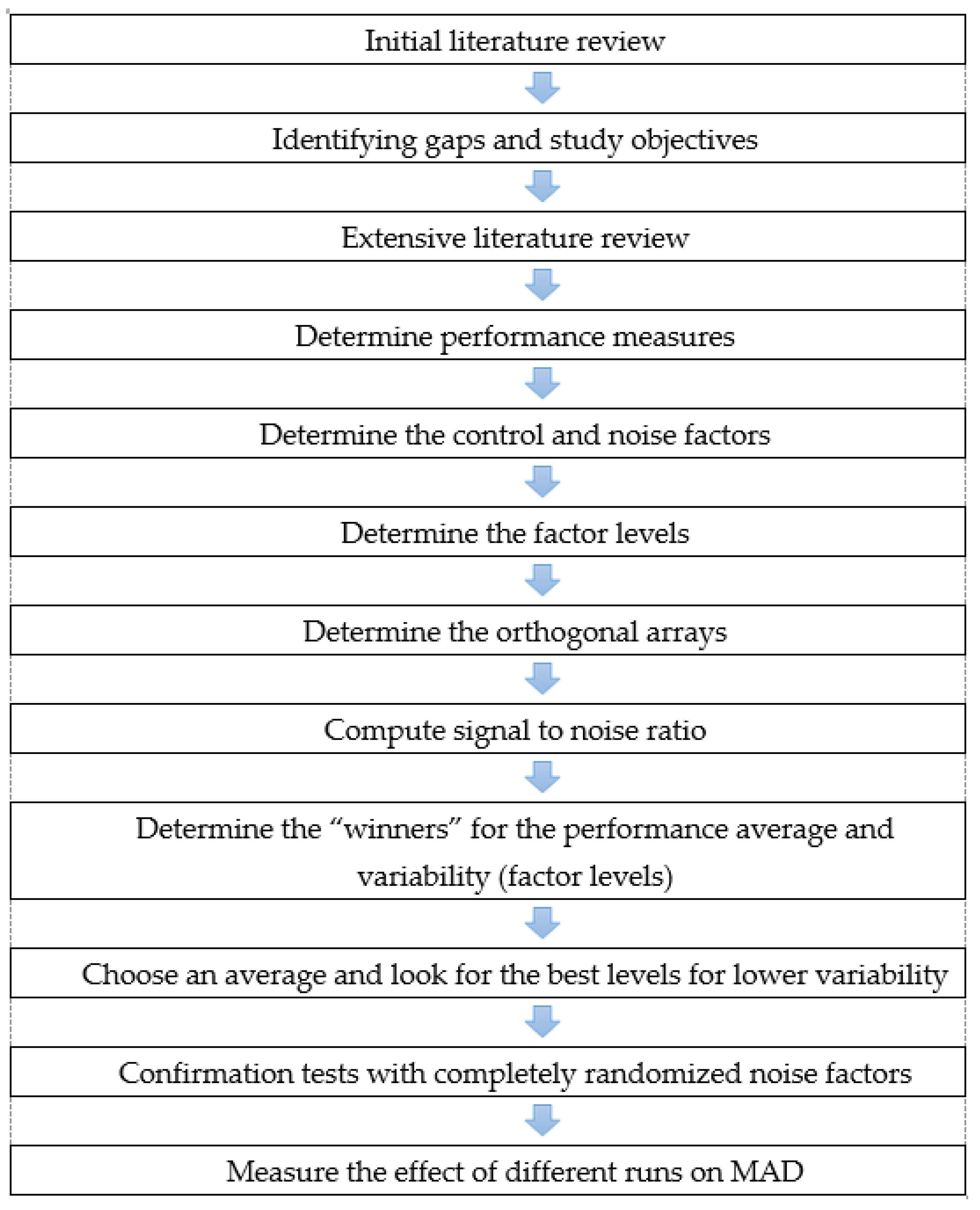
Figure 1 shows the steps of this study. Each step will be explained in this section and the next one.

2.2. Taguchi Method

The Taguchi method has been used successfully to improve the quality of Japanese products since 1960. However, in this paper, it will be used for the first time in developing the agreements of oil between the state and international companies. It is necessary to obtain the desired performance measures while minimizing the consequences of variation, but without eliminating the causes of this variation (since they are difficult to control). It is well-known that “A” and “B” factors affect the net present values of both parties [6]. The contribution of this study is to examine the effect of different levels of “A” and “B” factors on the variability of the profits of both parties. The main hypothesis is that there are some levels of control factors (“A” and “B” factors) that reduce the fluctuations in some targeted performance measures. In this study, the causes of variability are the oil price, the liquid hydrocarbon price (LHP), and gas price, which are very dynamic. The end result is a robust method that has the minimum sensitivity to variations in the uncontrollable noise factors (prices). In Taguchi’s parameter design approach, the outcome is influenced by two sorts of factors: control factors and noise factors. Control factors are those that can be easily controlled. Noise factors are those that are difficult, impossible, or expensive to control [26,27].

The objective of this research is to find the “A” and “B” values that make the agreement more robust against the fluctuations in the prices of oil, LHP, and gas. Robust agreements reduce the negotiation effort. The “A” and “B” levels are used to determine the net present value of the two parties in the agreement. The eight “A” and “B” factors (A1, A1, A3, A4, B1, B2, B3, and B4) are negotiable. This study can help decision makers while negotiating these values to look for better levels that are more robust against the changes in the prices and therefore to be fair for both sides. The ranges of the values of the control factors are relatively long, and therefore trying all the possible values is very time consuming. Therefore, it is better to choose some levels.

In Taguchi’s approach, the design of experimental techniques, particularly Orthogonal Arrays (OAs), are used to systematically modify and evaluate the varied values of each of the control factors. The columns in the OA represent the factor and its related levels, and each row in the OA represents an experimental run at the provided factor settings [26,27]. The eight “A” and “B” factors are the control factors. The experimental designer is responsible for determining the proper factor levels for each control factor. In this study, four levels were chosen for each one of the “A” and “B” factors.

Trying out all the combinations will give 65,536 (=4⁸) different possible runs. This is a time-consuming calculation. The Taguchi method depends on just trying some of these combinations using the proper OAs. Then, for each one of the runs, the noise combinations are tried. In this study, the noise factors are the changes in the oil price, LHP price, and gas price. Two levels were chosen for each of these noise factors: one for higher price and another one for lower prices. Some ranges of prices were chosen as shown in the lower part of

Table 4. Selected control and noise factors of the study.

Factor	Levels
A. Control factors	Level 1	Level 2	Level 3	Level 4
A1	0.9	0.92	0.94	0.96
A2	0.78	0.8	0.82	0.84
A3	0.55	0.6	0.65	0.7
A4	0.35	0.4	0.45	0.5
B1	0.90	0.92	0.94	0.96
B2	0.7	0.75	0.8	0.85
B3	0.55	0.6	0.65	0.7
B4	0.4	0.45	0.5	0.55
B. Noise factors	Level 1		Level 2
Oil price	80		90
LHP price	81		94
Gas price	4		5.33

. L8 represents the full OA for the noise factors in this study. Table 4 shows the different levels for both the control and noise factors.

L256 orthogonal design was chosen for control factors. This means that there were 256 different combinations of the levels of the control factor. Some of these runs were deleted because B3 and B4 have a similar level (0.55) in these runs. The number of remaining experimental runs was 224. As mentioned before, L8 was chosen for noise factors. R software was used to make the needed calculations.

Taguchi recommends using an “inner array” and “outer array” approach to build robust design. The “inner array” is the OA containing the control factor settings; the “outer array” is the OA containing the noise factors and their settings that are being investigated. The inner array and outer array are combined to form the “product array” or full parameter design layout. The product array is used to test various combinations of control factor settings across all noise factors in a systematic manner [26,27]. The total set of experiments is attained by combining the L224 array of control factors with the L8 array of noise factors. The total number of experiments is the product of the number of runs of outer and inner arrays (224 × 8 = 1792 experiments).

Table 5. Control and noise levels design (the first 10 runs).

				Outer Array (L8)			Oil price		90	90	80	90	80	90	80	80
							LHP price		94	81	94	94	81	81	94	81
							Gas price		4	4	5.33	5.33	5.33	5.33	4	4
	Inner Array (256)								Results
Run	A1	A2	A3	A4	B1	B2	B3	B4
1	0.9	0.8	0.65	0.5	0.96	0.8	0.6	0.4
2	0.9	0.78	0.7	0.4	0.96	0.85	0.7	0.55
3	0.94	0.8	0.55	0.5	0.9	0.85	0.55	0.45
4	0.96	0.78	0.55	0.5	0.9	0.8	0.6	0.55
5	0.9	0.84	0.55	0.5	0.9	0.75	0.65	0.5
7	0.94	0.82	0.7	0.4	0.96	0.75	0.6	0.4
9	0.92	0.8	0.6	0.5	0.9	0.8	0.55	0.5
10	0.96	0.84	0.6	0.4	0.94	0.85	0.65	0.55

shows the first 10 runs (control factors together with the noise factors). Results should be in the lower right part of the figure. Each run has eight experiments. For each run, the average, standard deviation, and signal-to-noise ratio were found. Factor levels that increase the SN ratio are the best. Larger SN ratios mean lower variability.

The SN ratio can be found as follows in Equation (12), where the aim is to keep the SN values around a desired target [26,27].

$$S{N}_T=10log\left(\frac{{\overline{y}}^2}{S^2}\right)$$

(12)

The higher the ratio, the lower the variability due to the noise factors (price fluctuations). The decision makers in the two parties will focus not only on reducing the fluctuations but also on the best profit for each party. The SN ratios must be computed for each run. The SN ratios and average responses can be plotted for each factor against each of its levels. The graphs are tested to choose the factor level which maximizes SN ratio and brings the mean on target. Generally, factors can affect both the variation and the average performance (just like the factors in this study) or one of them (average or variation), or do not affect either the variance or the average. Generally, reducing the variations in the system will make it more robust.

There are two response variables chosen in this study which are the average value of the second-party percent share of production (ASPS) and the percent of profit of the second party (SPP), which can be called “company take”. The percent of the profit of the first party (government take) is simply the same as the SPP. The second party percent share of production usually fluctuates between zero and the maximum second party share. Any small difference in this share makes a difference of millions of USD for both parties. Its value in the first few years is zero. The average value of the nonzero values is chosen to be the response variable, which is the ASPS. It is important to notice that two possible runs with the same ASPS does not guarantee that both of them have the same NPV. Therefore, SPP might be more interesting for the international company.

3. Results and Analysis

The results are shown for the two response variables.

3.1. First Response Variable: ASPS

Table 6. Results for the first 10 runs for ASPS.

	Noise Factors Runs
	1	2	3	4	5	6	7	8
Oil price	90	90	80	90	80	90	80	80
LHP price	94	81	94	94	81	81	94	81
Gas price	4	4	5.33	5.33	5.33	5.33	4	4
Run	Results								$\overline{\mathit{y}}$	S	$\mathit{S}{\mathit{N}}_{\mathit{T}}$
1	0.095	0.095	0.102	0.094	0.103	0.094	0.106	0.107	0.100	0.006	25.04
2	0.091	0.091	0.104	0.089	0.104	0.089	0.110	0.113	0.099	0.010	20.17
3	0.091	0.091	0.096	0.090	0.096	0.090	0.097	0.098	0.094	0.003	29.48
4	0.091	0.091	0.096	0.091	0.096	0.091	0.097	0.098	0.094	0.003	29.43
5	0.092	0.092	0.097	0.091	0.097	0.091	0.098	0.099	0.095	0.003	29.69
7	0.090	0.090	0.102	0.088	0.102	0.088	0.108	0.111	0.097	0.010	20.03
9	0.091	0.091	0.097	0.090	0.097	0.090	0.099	0.100	0.095	0.004	26.96
10	0.090	0.090	0.099	0.088	0.099	0.088	0.104	0.105	0.095	0.007	22.38

shows the initial results of the first 10 runs when the performance measure is ASPS. For example, ASPS (which is $\overline{y}$ in Table 6) for the first run is 10%. Moreover, the ASPS for the ninth and the tenth runs is the same, which is 9.5. However, the ninth run is more robust since its SN ratio is higher, and its standard deviation (S) is lower.

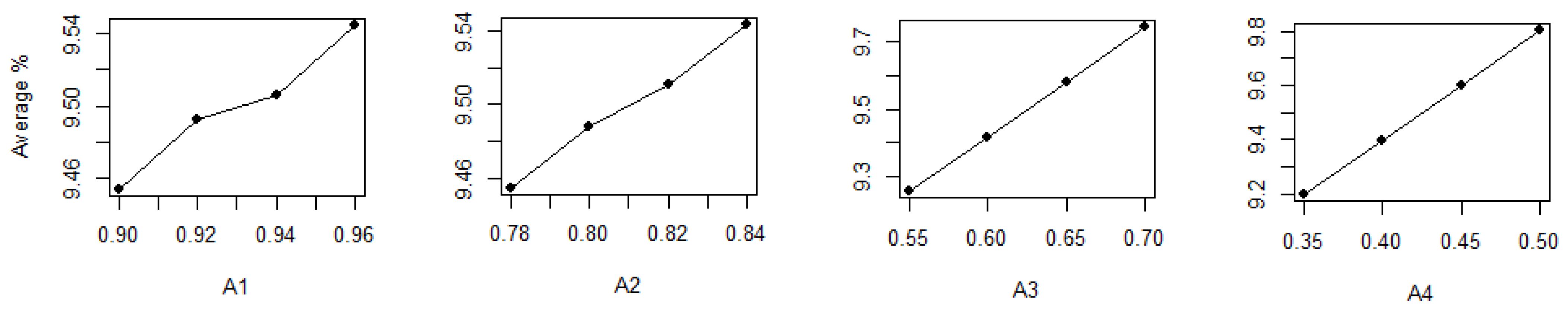
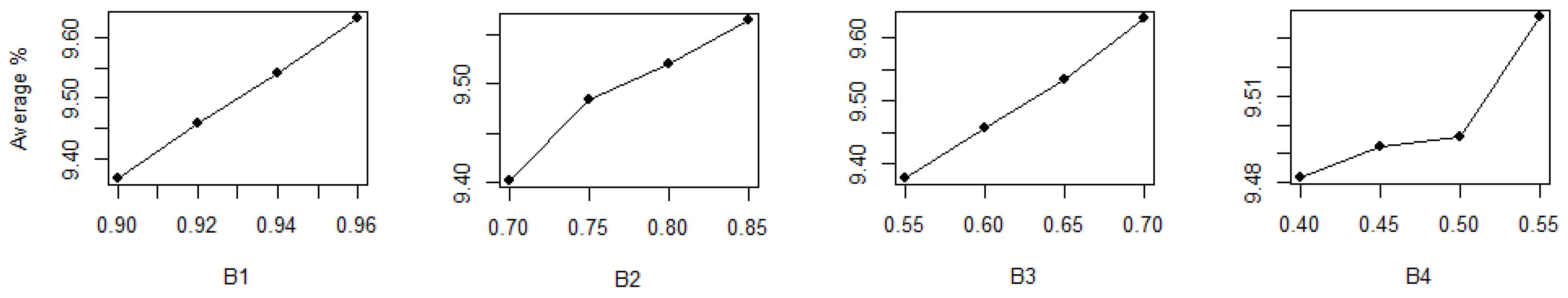
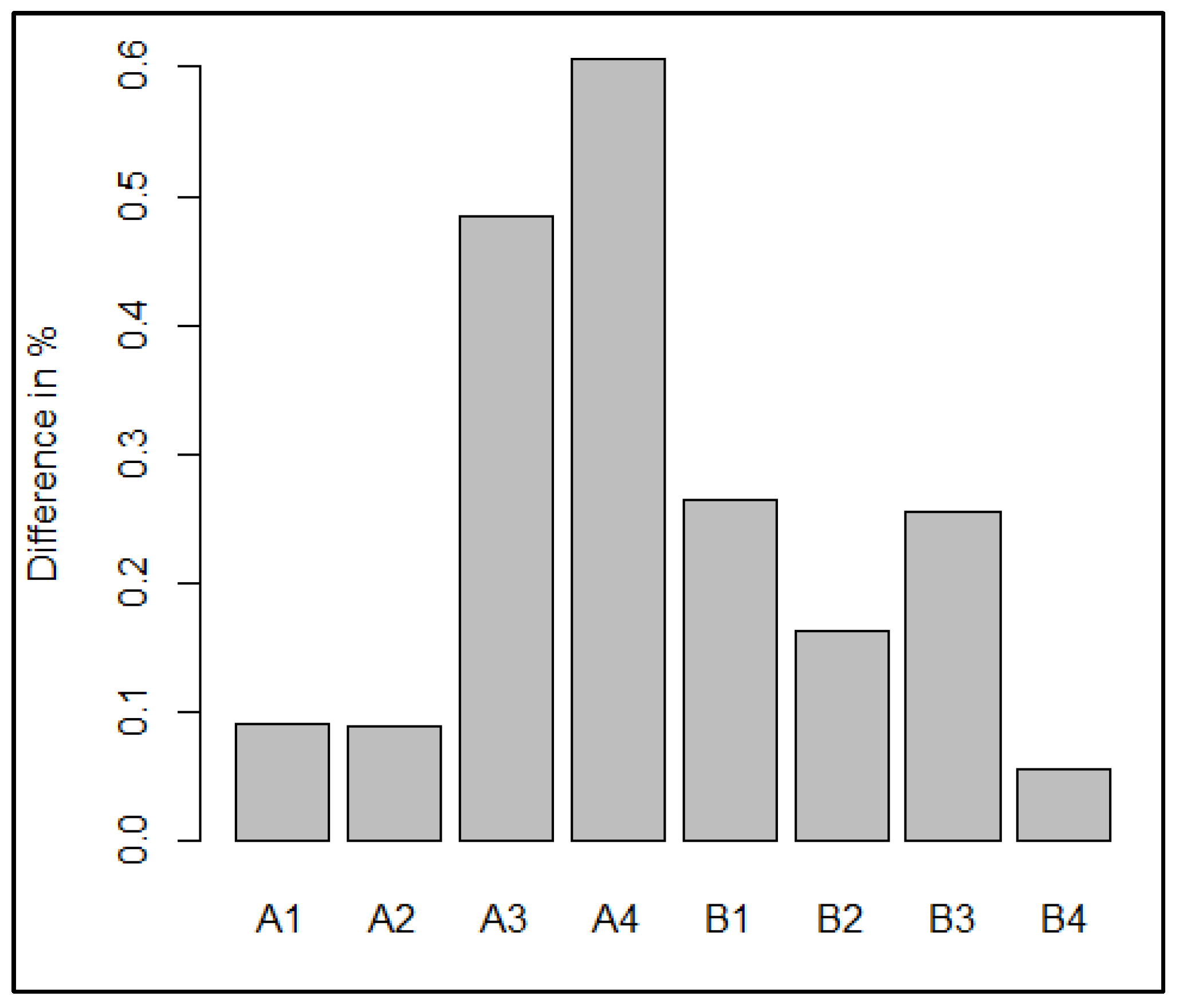
The complete results for the 224 runs were obtained in the same way. Figure 2 shows the effect of the “A” factors on the response variable (performance measure). It is computed by taking the average of the runs of control and noise factors. For example, for the “A1” factor, 56 runs are for each level of “A1” (0.9, 0.92, 0.94, and 0.96). For each one of these 56 runs, there are eight experiments associated with the noise L8. Therefore, there are 448 experiments for each level of “A1”. The average values of the 448 experiments are taken for each level. Figure 2 also shows the effect of “B” factors. It is clear that increasing the level for each factor of “A” and “B” will increase the response variable average, and therefore, it is better for the second party to increase the levels of the eight factors, but not for the first party. However, the effect of each of the eight factors is different. Figure 3 shows the difference in the impact between these factors on the average response variable. The figure shows that “A3” and “A4” make the greatest difference. This difference is calculated by finding the average of the maximum and the minimum levels of the response variables. For example, increasing the level of “A4” from 0.35 to 0.5 will increase ASPS from 9.2% to 9.8%.

When prices are higher, the response variable (ASPS) will be beneficial for the first party. Lower prices lead to a better response variable for the second party, but lower NPV for both parties. The average response variable ASPS was found to be 10.47% for lowest prices and 8.79% for the highest prices. Besides the average values found in Figure 2, another direction to be considered is the robustness, where the effect of the noise factors is the lowest for some certain levels. Figure 4 shows these levels.

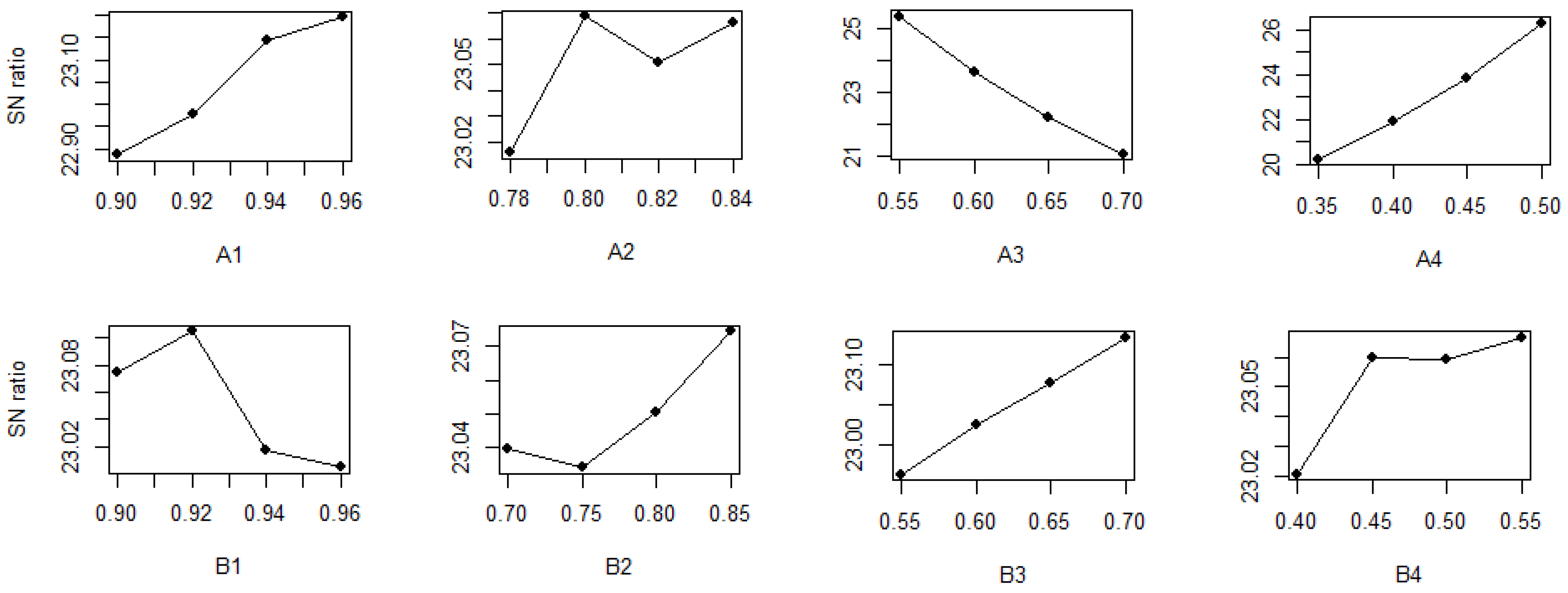
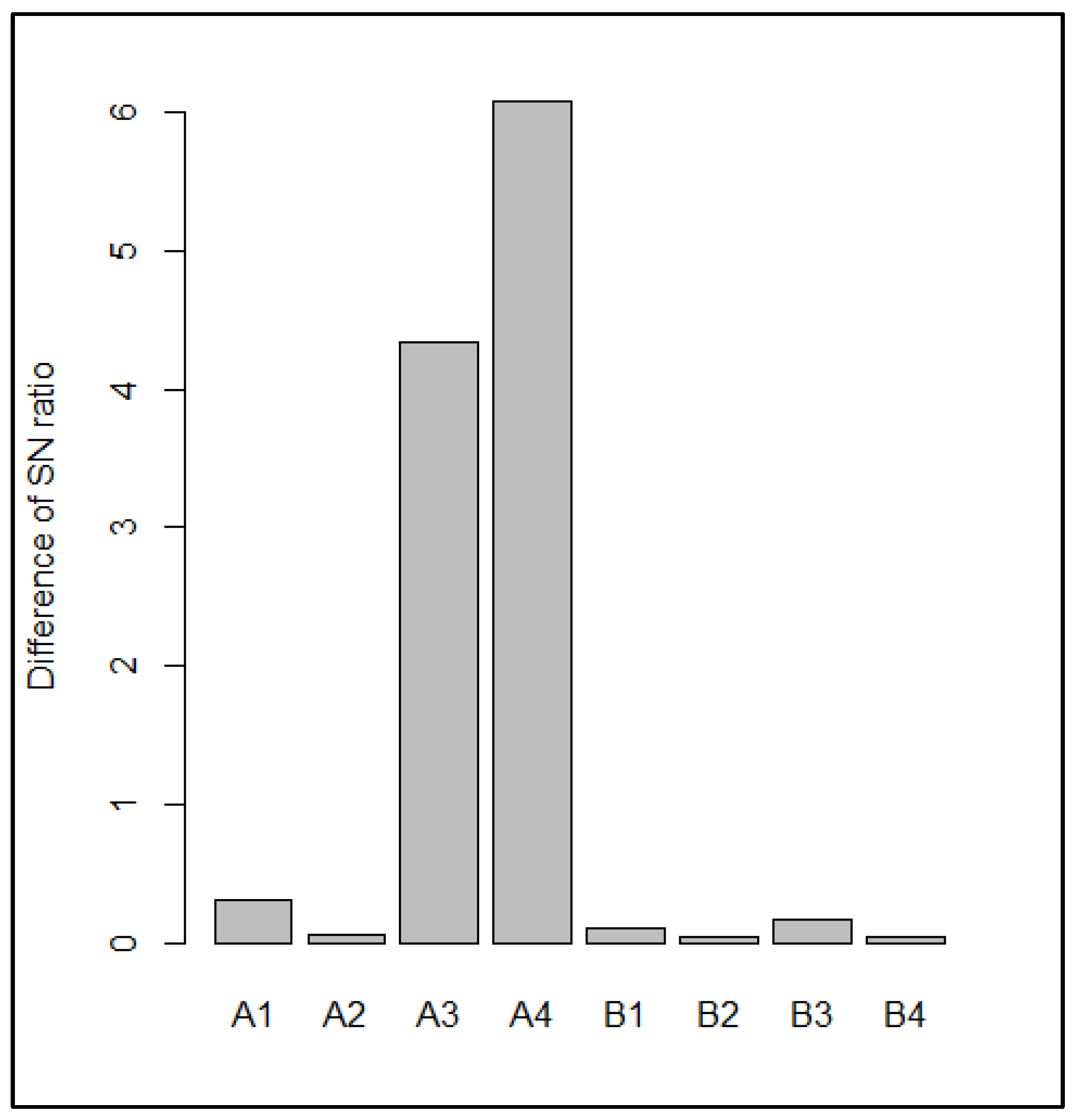
According to Figure 4, generally, the higher the level for “A” factors, the lower the variability, except for with “A3”. Moreover, for “B” factors, only “B1” needs to be decreased to obtain lower variability. The maximum effect that each factor can have on SN ratio can be found by estimating the difference between the maximum and minimum y-axis values in Figure 4. Figure 5 shows these ranges. “A3” and “A4” have the highest effect on the variability of the response variable.

Assume that both parties agreed on obtaining an average response value of 9.51% plus or minus 0.01%.

Table 7. Possible combinations of factor levels to obtain a 9.51% target of ASPS.

Run	A1	A2	A3	A4	B1	B2	B3	B4	$\overline{\mathit{y}}$	SN Ratio	Range
1	0.9	0.78	0.7	0.35	0.94	0.75	0.7	0.5	9.50%	18.83	2.63
2	0.9	0.82	0.6	0.45	0.96	0.75	0.55	0.5	9.51%	24.38	1.37
4	0.96	0.82	0.6	0.4	0.96	0.85	0.6	0.45	9.51%	22.26	1.75
5	0.94	0.82	0.6	0.4	0.94	0.8	0.7	0.45	9.52%	22.42	1.72
6	0.9	0.78	0.6	0.5	0.9	0.85	0.6	0.4	9.52%	27.04	1.00

shows the possible different combinations of factor levels used to reach the target. It is very clear that the last row represents the best solution with the highest SN ratio and the lowest range. The range is the maximum value minus the minimum value. This is another way to represent variability. Generally, larger ranges lead to smaller SN ratios. The last run is the fairest solution. This is because “A4” has the highest value. As previously mentioned in Figure 4, increasing “A4” will lead to lower variability.

3.2. The Second Response Variable: Company Take (SPP)

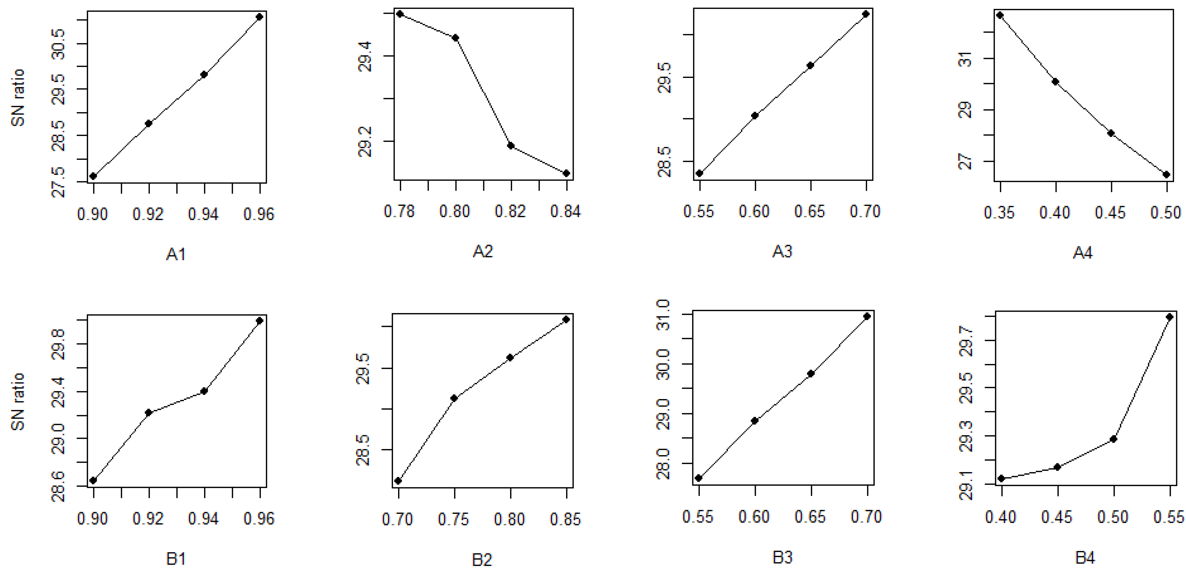
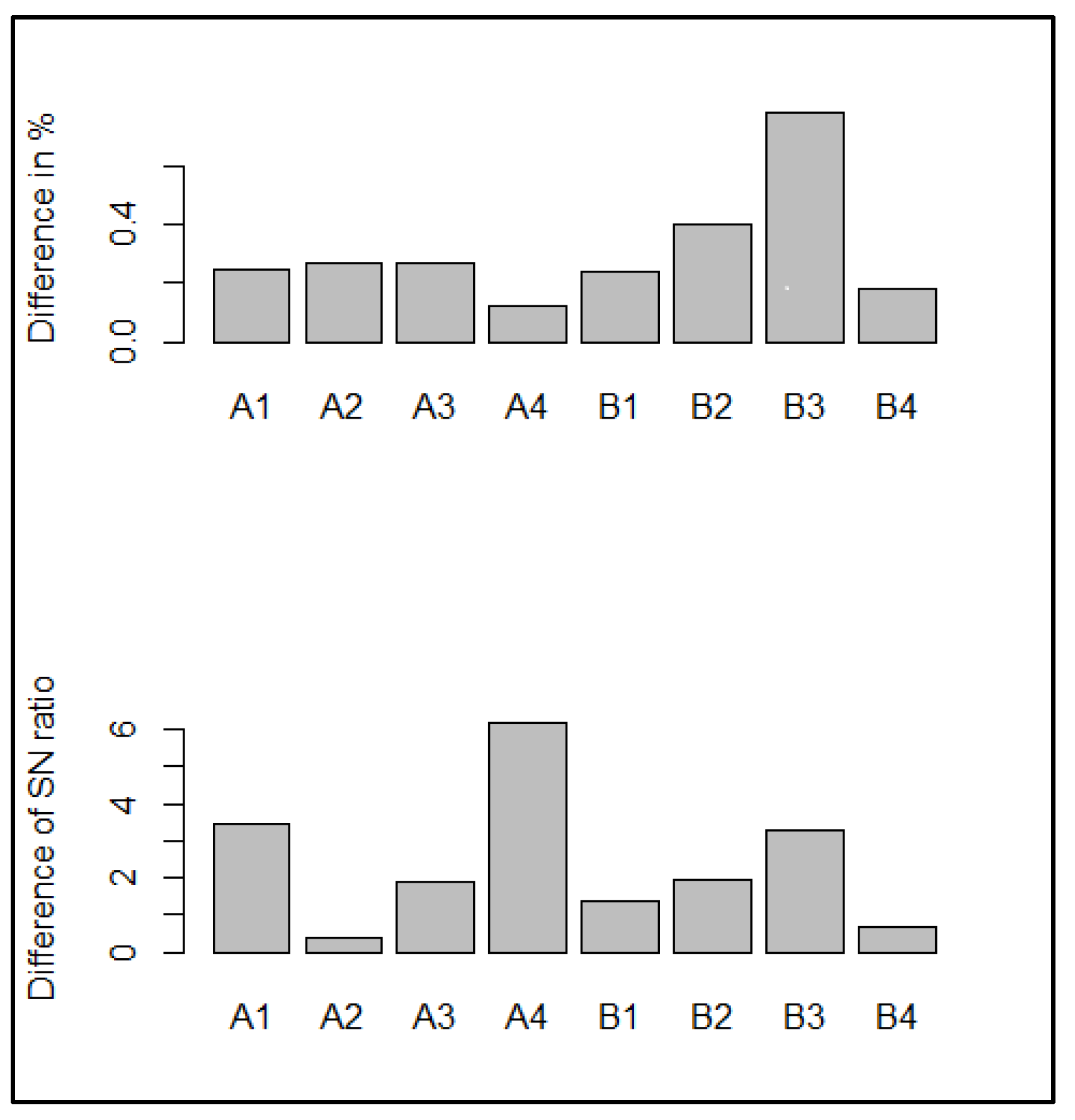
Changing the response variable can have different results. The decision maker must decide which variable to take. For example, SPP can be the response variable, and the effects of the control factors are shown in Figure 6. For “A2” and “A4”, the larger the level, the higher the variability (lower SN ratios). However, for the other factors, the larger the level, the lower the variability. Figure 7 shows that while “A4” does not have a large effect on the average response variable, it has indeed the largest effect on stabilizing the fluctuations in the response variable.

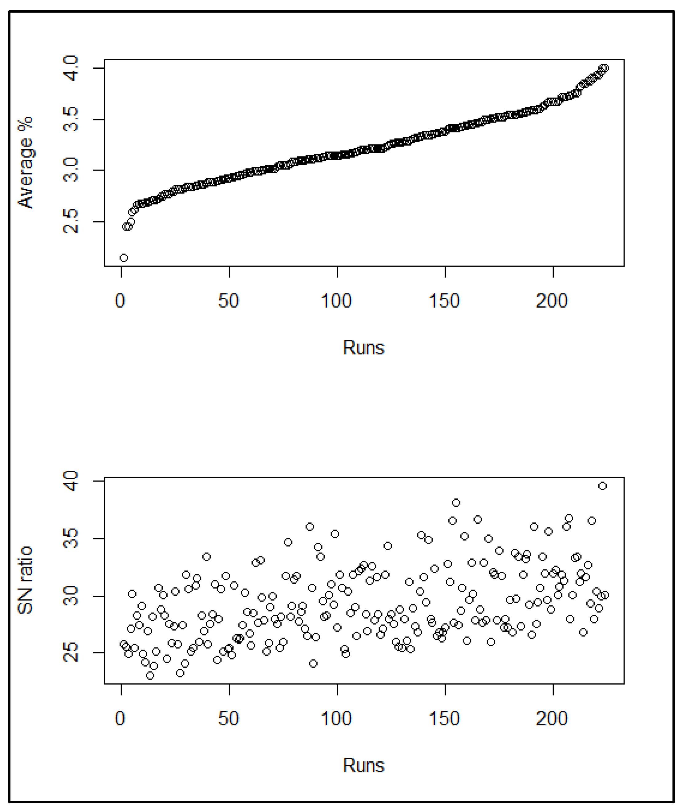
Usually, higher prices will give a higher percent of profit for the second party (3.34% in this case), while higher prices will give a lower percent of production share to the second party (3.08% in this case). Different combinations of the “A” and “B” factors levels have a great effect on SPP. Figure 8 shows this effect. It is very interesting to see that adjacent runs with almost the same average response variable have different SN ratios, which means even when two options have the same average, one of them can better reduce the fluctuations in the response variable due to price fluctuations.

Assume that the two parties agreed to obtain an average of 3.21% for SPP. There are different ways to have the same average value within the assumed prices ranges.

Table 8. Possible runs with an average of 3.21% for SPP.

Run	A1	A2	A3	A4	B1	B2	B3	B4	$\overline{\mathit{y}}$	SN Ratio	Range
1	0.92	0.84	0.6	0.35	0.92	0.85	0.6	0.5	3.21	31.26	0.2
2	0.96	0.78	0.7	0.4	0.9	0.7	0.65	0.55	3.21	32.59	0.18
3	0.92	0.78	0.55	0.45	0.96	0.8	0.65	0.5	3.21	27.86	0.32
4	0.96	0.84	0.7	0.4	0.96	0.7	0.55	0.5	3.21	31.58	0.2
5	0.9	0.8	0.55	0.4	0.9	0.8	0.7	0.55	3.21	28.36	0.3
6	0.94	0.8	0.65	0.5	0.92	0.7	0.65	0.4	3.21	26.66	0.35

shows some of these possible ways. The second combination of factors’ levels gives the best results because it is more immune to the fluctuations in the prices. This is obvious in the SN ratio, which is the maximum, and the range, which is the minimum. Compared to the worst combination (in the last run: 0.35), the range is almost the double the 0.18 of run number 2.

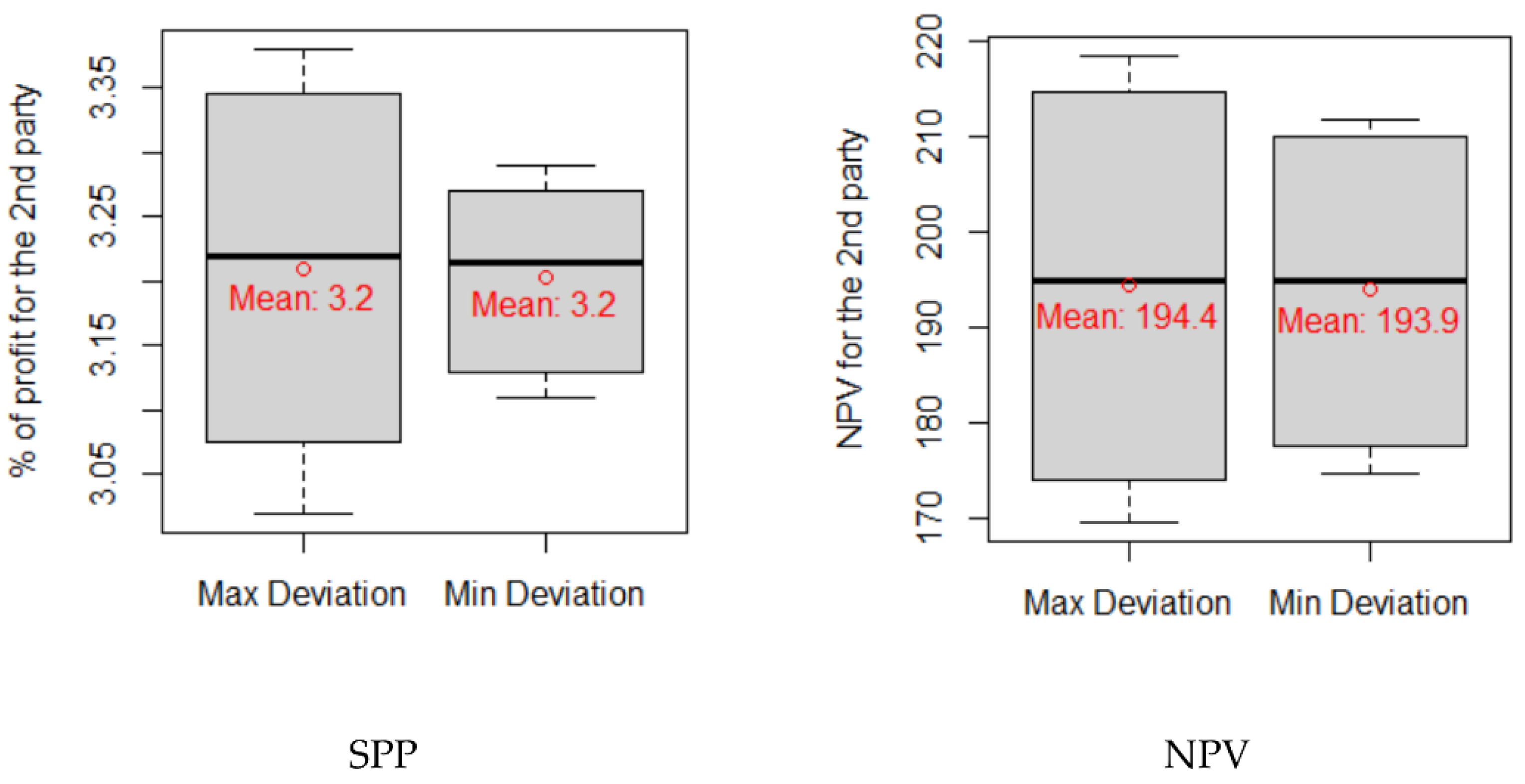
Figure 9 shows the variability for the best and worst runs found in the previous table. Each boxplot has eight values. Boxplots usually show the minimum, Q1 (First Quartile), median, Q3 (third Quartile), and maximum. The wider the box, the more variability (fluctuation) the response variables have. The purpose of the figure is to check the effect of choosing the right combinations on the NPV. As expected, the variability in SPP is more for the run with the maximum deviation (the last run in Table 6). The same conclusion about variability is found for NPV in the right side of the figure.

Table 9. Comparison between a randomly selected run and two runs of the selected sample.

Run	Control Factors								SPP	NPV
	A1	A2	A3	A4	B1	B2	B3	B4		Average (USD MM)	Standard Deviation (USD MM)	SN Ratio
Min deviation	0.96	0.78	0.7	0.4	0.9	0.7	0.65	0.55	3.21%	193.91	17.30	20.99
Max deviation	0.94	0.8	0.65	0.5	0.92	0.7	0.65	0.4	3.21%	194.44	21.84	18.99
Randomly selected	0.9	0.78	0.6	0.5	0.9	0.85	0.6	0.4	2.83%	171.61	21.90	17.88

shows a comparison between a randomly selected run and the other two runs with the average company take of 3.21%. Results show that the effect of the control factors is significant on the average and the variability of the NPV. A difference of less than 0.4% on SPP means a difference of more than USD 22 MM on the NPV. The effect of “A” and “B” factors on the NPV was previously reported by Balhasan and Biltayib [6] and Balhasan et al. [14]. However, this paper is the first one that uses a design-of-experiment method to investigate the effect, not only on the average of but also on the variability in response variables due to the noise factors.

In the above results, however, it is assumed that there are only two possible prices (the minimum and the maximum) and that they are fixed all the time. However, in reality, prices are always changing. Therefore, it is better to compare the two scenarios (maximum and minimum deviations) with completely randomized prices within the given ranges. This was performed using 1000 combinations of prices instead of the 8 in L8, and the results in

Table 10. Mean absolute deviation (MAD) values for random prices (1000 trials).

Run and Control Factors	MAD Values of NPV
1. Best combinations (Min deviation) A1  A2  A3  A4  B1  B2  B3  B4 0.96 0.78 0.7 0.4 0.9 0.7 0.65 0.55	3.83 MM
2. Worst combinations (Max deviation) A1  A2  A3  A4  B1  B2  B3  B4 0.94 0.8 0.65 0.5 0.92 0.7 0.65 0.4	4.65 MM

were obtained where mean absolute deviation (MAD) is used to estimate the performance (the robustness). Higher MAD means more variability. The meaning of the results is that, on average, the fluctuations in prices make a deviation of 3.83 MM for the best combinations of factors levels, and 4.65 MM around the average for the worst combinations of factors levels. Therefore, in the best run, the profitability is shared between the two parties, with somewhat smaller differences from one year to another.

The reduction in MAD (from USD 4.65 MM to USD 3.83 MM) for NPV for the second part is about 18%. As mentioned earlier, higher “A1” is generally better, and this is obvious in the table (0.96 is better than 0.94). Lower “A4” (0.4 in the table) is generally better than higher values (0.5 in the table). “B3” in both of them has the same value.

3.3. Managerial Implications

The study helps decision makers in the field of exploration of oil to find a way to look for a fair contract that is more robust against the fluctuations in the prices. The state and the international company can set the “A” and “B” factors in a way that gives a negotiable economic indicator (on average). However, the value of this economic indicator is obtained if prices are within a certain range. Some changes in prices will be good for one party at the expense of the other, and in most cases, it will be in the government’s interest. More fair agreements are needed. The methodology used in the paper can easily be applied since the computation time is very short, and the Taguchi method is popular and practical. It is true that R software was used in this study for research purposes, but there are different software programs that can be used to obtain the results. Different combinations of “A” and “B” factors can give the same average of the economic indicator, but with different variability. One of these combinations gives the lowest variability, and that is what this study investigates. For example, it was found based on the given data in the case study that to obtain the most robust results, A3 and A4 are the most important factors needed to reduce variability in ASPS, while A1, A4, B3 are the most important factors needed to reduce variability in company take. Robust results of ASPS can be obtained by decreasing the levels of A3 and B1 and increasing the others, while robust outputs of company take can be obtained by decreasing A2 and A4 and increasing the others. However, different results can be obtained for other case studies with different data. Knowing such information makes it easier for both parties in negotiation of the conditions of the contract.

4. Conclusions

In this study, the effect of fluctuations in oil, LHP, and gas prices on the fairness of the contracts in the oil exploration industry is investigated. The best parameters (“A” and “B” factors) that reduce the effect of the noise factors on the company take and ASPS were investigated. Some parameters were found more important than the others on increasing the signal-to-noise (SN) ratios, and therefore reducing the variability. The results revealed that the most important control factors affecting the ASPS are A3 and A4, while the most important control factors affecting the company (IOC) take are B2 and B3. The most important factors to reduce variability in ASPS are A3 and A4, while the most important factors to reduce variability in company take are A1, A4, and B3. ASPS’ results can be made more robust by lowering the levels of A3 and B1 and raising the others, while company take outputs can be made more robust by lowering the levels of A2 and A4 and raising the others. If the two parties of the contract agreed on a certain value of company take, then different combinations of the eight “A” and “B” factors can lead to the same company take. However, some combinations are better than the others based on obtaining lower variability due to the price fluctuations. About an 18% reduction in the variability of NPV, which was measured by MAD, was found when the average company take was 3.21%.

There are some limitations in the study. For example, the data are for a case study in Libya. Different optimal levels can obtained for different data. The analysis also depends on only two levels of the prices to reduce the calculation efforts. More levels or ranges can be helpful. Future research can check the effect of changing the “A” and “B” levels after the beginning of the contract by some years.

References

- Ahmadov, I.; Artemyev, A.; Aslanly, K.; Rzaev, I.; Shaban, I. How to Scrutinise a Production Sharing Agreement. A Guide for the Oil and Gas Sector based on the Experience from the Caspian Region; International Institute for Environment Development (IIED): London, UK; Soros Foundation-Kazakhstan: Almaty, Kazakhstan; Public Finance Monitoring Center (PFMC): Baku, Azerbaijan, 2012. [Google Scholar]
- Al Shehhi, A.; Al Hazza, M.; Alnahhal, M.; Sakhrieh, A.; Al Zarooni, M. Challenges and Barriers for Renewable Energy Implementation in the United Arab Emirates: Empirical Study. Int. J. Energy Econ. Policy 2021, 11, 158. [Google Scholar] [CrossRef]
- Ali, S.F.; Yusoff, N. Determination of Optimal Cut Point Temperatures at Crude Distillation Unit Using the Taguchi Method. Int. J. Eng. Technol. 2012, 12, 36–46. [Google Scholar]
- Balhasan, S.A.; Towler, B.F.; Miskimins, J.L. Modifying the Libyan fiscal regime to optimise its oil reserves and attract more foreign capital part 1: LEPSA I proposal. OPEC Energy Rev. 2013, 37, 220–246. [Google Scholar] [CrossRef]
- Balhasan, S.A.; Towler, B.F.; Miskimins, J.L. Modifying the Libyan fiscal regime to optimise its oil reserves and attract more foreign capital part 2: Application to CO2-EOR project in Libya. OPEC Energy Rev. 2013, 37, 270–313. [Google Scholar] [CrossRef]
- Balhasan, S.A.; Towler, B.F.; AlHadramy, K.O.; Biltayib, B.M. Comparative risk evaluation and sensitivity analysis of the Libyan EPSA IV and its modified model LEPSA I. Petroleum 2020, 6, 206–213. [Google Scholar] [CrossRef]
- Balhasan, S.; Biltayib, B. Risk Evaluation & Sensitivity Analysis of the Exploration & Production Sharing Agreement. In Proceedings of the Abu Dhabi International Petroleum Exhibition & Conference, Abu Dhabi, United Arab Emirates, 11–14 November 2019. [Google Scholar]
- Balhasan, S.; Misbah, B.; Omar, M.; Musbah, I.; Khameiss, B. Impact of Proposal Changes to Libyan Oil Taxation System on Developing the 137 B Offshore Field. J. Eng. Appl. Sci. 2018, 13, 6085–6090. [Google Scholar]
- BenZeglam, M.S. Development and Evaluation of an Economic Model for a Libyan Oil Field Development with an EPSA Agreement. Master’s Thesis, West Virginia University, Morgantown, WV, USA, 2018. [Google Scholar] [CrossRef] [Green Version]
- Bindemann, K. Production-Sharing Agreements: An Economic Analysis; Oxford Institute for Energy Studies: Oxford, UK, 1999. [Google Scholar]
- Boopathi, S. Experimental investigation and parameter analysis of LPG refrigeration system using Taguchi method. SN Appl. Sci. 2019, 1, 1–7. [Google Scholar] [CrossRef] [Green Version]
- Chen, W.; Allen, J.K.; Tsui, K.L.; Mistree, F. A Procedure for Robust Design: Minimizing Variations Caused by Noise Factors and Control Factors. J. Mech. Des. 1996, 118, 478–485. [Google Scholar] [CrossRef] [Green Version]
- Cheng, S.W.; Kurnia, J.C.; Ghoreishi-Madiseh, S.A.; Sasmito, A.P. Optimization of geothermal energy extraction from abandoned oil well with a novel well bottom curvature design utilizing Taguchi method. Energy 2019, 188, 116098. [Google Scholar] [CrossRef]
- Ding, Y.; Liu, Y.; Failler, P. The Impact of Uncertainties on Crude Oil Prices: Based on a Quantile-on-Quantile Method. Energies 2022, 15, 3510. [Google Scholar] [CrossRef]
- Diouf, A.; Laporte, B. Oil contracts and government take: Issues for Senegal and developing countries. J. Energy Dev. 2017, 43, 213–234. [Google Scholar]
- Dirani, F.; Ponomarenko, T. Contractual Systems in the Oil and Gas Sector: Current Status and Development. Energies 2021, 14, 5497. [Google Scholar] [CrossRef]
- Durrani, M.; Ahmad, I.; Kano, M.; Hasebe, S. An Artificial Intelligence Method for Energy Efficient Operation of Crude Distillation Units under Uncertain Feed Composition. Energies 2018, 11, 2993. [Google Scholar] [CrossRef] [Green Version]
- Ebrahimi, H.; Kianfar, K.; Bijari, M. Scheduling a cellular manufacturing system based on price elasticity of demand and time-dependent energy prices. Comput. Ind. Eng. 2021, 159, 107460. [Google Scholar] [CrossRef]
- Hossain, M.A.; Chakrabortty, R.K.; Ryan, M.J.; Pota, H.R. Energy management of community energy storage in grid-connected microgrid under uncertain real-time prices. Sustain. Cities Soc. 2021, 66, 102658. [Google Scholar] [CrossRef]
- Hussein, M.; Kareem, I. Optimising the chemical demulsification of water-in-crude oil emulsion using the Taguchi method. IOP Conf. Ser. Mater. Sci. Eng. 2020, 987, 012016. [Google Scholar] [CrossRef]
- Johnston, D. International Exploration Economics, Risk and Contract Analysis; Pennwell: Tulsa, OK, USA, 2003. [Google Scholar]
- Kolovrat, M.; Jukić, L.; Sedlar, D.K. Comparison of Hydrocarbon Fiscal Regimes of Some European Oil and Gas Producers and Perspectives for Improvement in the Republic of Croatia. Energies 2021, 14, 5056. [Google Scholar] [CrossRef]
- Li, Z.; Huang, Z.; Failler, P. Dynamic Correlation between Crude Oil Price and Investor Sentiment in China: Heterogeneous and Asymmetric Effect. Energies 2022, 15, 687. [Google Scholar] [CrossRef]
- Lyu, Y.; Yi, H.; Wei, Y.; Yang, M. Revisiting the role of economic uncertainty in oil price fluctuations: Evidence from a new time-varying oil market model. Econ. Model. 2021, 103, 105616. [Google Scholar] [CrossRef]
- Mian, A. Project Economics and Decision Analysis: Deterministic Models, 2nd ed.; PennWell Corporation: Tulsa, OK, USA, 2011. [Google Scholar]
- Romasheva, N.; Dmitrieva, D. Energy Resources Exploitation in the Russian Arctic: Challenges and Prospects for the Sustainable Development of the Ecosystem. Energies 2021, 14, 8300. [Google Scholar] [CrossRef]
- Setak, M.; Fozooni, N.; Daneshvari, H. Developing a model for pricing and control the inventory of perishable products with exponential demand. Int. J. Ind. Syst. Eng. 2019, 12, 120–140. [Google Scholar]
- Shen, Y.; Shi, X.; Zeng, T. Uncertainty, Macroeconomic Activity and Commodity Price: A Global Analysis. 2018. Available online: https://ssrn.com/abstract=3280848 (accessed on 1 July 2022).
- Stermole, F.J.; Stermole, J.M. Economic Evaluation and Investment Decision Methods; Investment Evaluations Corporation: Denver, CO, USA, 2006. [Google Scholar]
- Swe, W.T.; Emodi, N.V. Assessment of Upstream Petroleum Fiscal Regimes in Myanmar. J. Risk Financial Manag. 2018, 11, 85. [Google Scholar] [CrossRef] [Green Version]
- Tsui, K.L. An overview of Taguchi method and newly developed statistical methods for robust design. IIE Trans. 1992, 24, 44–57. [Google Scholar] [CrossRef]
- Urum, K.; Pekdemir, T.; Gopur, M. Optimum conditions for washing of crude oil-contaminated soil with bio surfactant solutions. Process Saf. Environ. Prot. 2003, 81, 203–209. [Google Scholar] [CrossRef]
- Yang, L. Connectedness of economic policy uncertainty and oil price shocks in a time domain perspective. Energy Econ. 2019, 80, 219–233. [Google Scholar] [CrossRef]
Figure 1.
Study Methodology.
Figure 2.
Effect of A and B factors on ASPS.
Figure 3.
The difference that each factor makes.
Figure 4.
Effect of A and B factors on the variability of SPS due to noise factors.
Figure 5.
Effect of A and B factors on the SN ratio.
Figure 6.
Effect of “A” and “B” factors on SN ratio for SPP.
Figure 7.
Effect of “A” and “B” factors on average (in %) and the SN ratio of SPP.
Figure 8.
The effect of factors’ levels on the variability (SPP).
Figure 9.
The variability in the best and worst runs in the chosen sample (3.21% for SPP).