Evolutionary Multi-Objective Optimization Applied to Industrial Refrigeration Systems for Energy Efficiency

Abstract

Refrigeration systems based on cooling towers and chillers are widely used equipment in industrial buildings, such as shopping centers, gas and oil refineries and power plants, among many others. Cooling towers are used to recover the heat rejected by the refrigeration system. In this work, the refrigeration is composed of cooling towers dotted with ventilators and compression chillers. The growing environmental concerns and the current scenario of scarce water and energy resources have lead to the adoption of actions to obtain the maximum energy efficiency in such refrigeration equipment. This backs up the application of computational intelligence to optimize the operating conditions of the involved equipment and cooling processes. In this context, we utilize multi-objective optimization algorithms to determine the optimal operational setpoints of the cooling system regarding the cooling towers, its fans and the included chillers. We use evolutionary multi-objective optimization to provide the best trade-offs between two conflicting objectives: maximization of the effectiveness of the cooling towers and minimization of the overall power requirement of the refrigeration system. The optimization process respects the constraints to guarantee the correct and safe operation of the equipment when the evolved solution is implemented. In this work, we apply three evolutionary multi-objective algorithms: Non-dominated Sorting Genetic Algorithm (NSGA-II), Micro-Genetic Algorithm (Micro-GA) and Strength Pareto Evolutionary Algorithm (SPEA2). The results obtained are analyzed under different scenarios and models of the cooling system’s equipment, allowing for the selection of the best algorithm and best equipment’s model to achieve energy efficiency of the studied refrigeration system.

1. Introduction

The technical and scientific community is moving fast towards adopting premises and drastic measures that allow the achievement of a maximal level of energy efficiency of industrial installations. This is due to the ever growing environmental concerns regarding the inefficient electrical power usage and its ever growing demand, as well as to the misuse of water resources. So, in order to achieve energy efficiency in industrial refrigeration systems, we require the utilization of modern mechanisms and methodologies that allow yielding a good or maybe the best possible solution for a process. Many industrial processes generate unwanted heat. So, this heat often must be somehow dissipated. In this case, water is generally used. The returning water in refrigeration systems is often at higher temperatures. It can be discarded or cooled down for further usage. However, the disposal of water is an environmentally unsustainable practice. Furthermore, the disposal of water, which comes at a high temperature would have a very negative impact on the local underwater flora and fauna. Hence, modern sustainable refrigeration system must be designed, configured and operated to reuse water. It is noteworthy to point out that there are more advanced refrigeration systems that are based on the usage of cryogenic fluids [1]. These kind of systems also aim at achieving high degrees of energy efficiency as required in critical systems, such as spaceships and nuclear stations [2]. An interesting survey of refrigeration methods can be found in [3].

Cooling towers are the basic equipment of industrial refrigeration systems. They are intended whenever there are large cooling demands. Moreover, cooling towers offer a clean and economical solution to water reuse in the cooling process. A cooling tower operates together with other equipment such as fans, chillers and pumps to ensure water circulation in the system [4,5]. A coordinated configuration of all the equipment composing the cooling system must be guaranteed. This is because a modification of some parameter in one of these equipment items can impact either positively or negatively the performance of the others parts of the system. When the cascading effects are unsatisfactory to the refrigeration system, a reduction of energy efficiency is often observed.

In this work, we propose to exploit computational intelligence techniques to optimize the energy requirement and effectiveness of an industrial refrigeration system composed of cooling towers, tower ventilators and chillers. For this purpose, quantitative and qualitative data are required to achieve good results. These data are usually collected from field data and data-sheets provided by the equipment manufacturers.

The attainable energy efficiency of a cooling tower is intrinsically dependent on that of the heat exchange process between the returning hot water and the air volume induced in counter-flow to this in the tower via ventilators. It is also influenced by climatic and operational aspects. This optimization is a complex process, and is mainly dependent on the precision of the model used for the equipment of the overall system.

The multi-objective optimization is two-fold. It aims at maximizing the efficiency of the heat exchange performed by the cooling tower while minimizing the global energy requirement of the refrigeration system. The optimization takes into account all the equipment necessary for the correct and safe operation of the refrigeration system. In this work, three evolutionary multi-objective optimization algorithms are applied: NSGA-II, Micro-GA and SPEA2. These algorithms will deliver the optimal settings of the system’s parameters to configure the composing cooling towers, tower fans and chillers. Mainly, the variables for which the optimization process will answer for are the cooling tower fan speed setpoint and the water temperature setpoint to be provided by the chillers. It is needless to state that the proposed optimization respects the restrictions imposed for a proper and safe operation of all the involved equipment composing the refrigeration system. The restrictions are set as provided by the equipment suppliers. The cooling system used in this work is based on compression chillers. Herein, such chillers are modeled in two different ways: a simple model wherein only one variable is considered and a more complete one wherein two variables are taken into account. The results yielded from both models are compared in terms of accuracy with respect to the field data. The two models provided for the chillers are used to set up the two objective functions for the optimization process. We also explore two different scenarios regarding the stopping criteria of the optimization algorithms. The performance results using different models and stopping criteria are compared, allowing the selection of the best algorithm for each scenario and the best model for the application.

This paper is structured into six sections. First, in Section 2, we briefly introduce the structure of the studied refrigeration system. Then, in Section 3, we provide a review of related research works. In the sequel, in Section 4, we define the objective functions and operational restrictions. After that, in Section 5, we describe the methodology behind each of the optimization algorithms applied in this work. Then, in Section 6, we analyze the evolved results for different algorithms, stopping scenarios and system models. Subsequently, in Section 7, we compare the effectiveness and efficiency of the used algorithm regarding the achievement of the main objective, which is the energy efficiency of the refrigeration system. Finally, in Section 8, we draw some conclusions and point out some promising directions for future work.

2. System’s Structure

The refrigeration system to be optimized is composed of chillers and cooling towers. This configuration is commonly used in commercial buildings and industrial facilities to ensure the thermal comfort of the transiting people and adequate equipment cooling and electrical rooms. The configuration of the cooling system considered in this work is presented in Figure 1. It includes two cooling towers, each composed of three elementary cells. Each cell includes a fan operating with an electric motor. Considering all the components composing the cooling tower, only the fans allow speed variation, through the use of frequency converters, while the others always remain operating at a fixed speed and equal to the nominal one.

In the case under study, the number of condensation water lift pumps in operation must be equal to the number of chillers in operation. Hence, the total number of cells in operation in the cooling towers can also be obtained based on the number of chillers in operation.

Among the equipment that composes the refrigeration system considered in this work, only the tower fans allow speed variation, through the use of frequency converters. Lift pumps and chillers operate at fixed speed, which is equal to the rated speed. Thus, as the condensed water pumps are not influenced by the speed variation of the tower fans, nor by the variation in the temperature of the water passing through the chillers, both in the condenser and in the evaporator, the required energy cannot be taken into account in the optimization process. Therefore, the optimization will be dedicated to the electrical energy demand of the fans and the chillers.

3. Related Works

In [6], the energy efficiency of the refrigeration system is achieved through a control strategy based on extreme search. The proposed control system is based on the global energy requirements, composed of chillers and tower fans. It attempts to reach energy efficiency exploiting variation of the fan speed setpoint. In [7], an extreme search strategy very similar to that presented in [6] is presented. The variable manipulated by the control system is the cooling tower output temperature, in contrast with the work reported in [6]. It exploits the tower ventilators. The achieved improvements vary in function of the chiller’s thermal load.

In [8], a control strategy called Optimum Approach Temperature (OAT) is proposed for the energy optimization of the cooling tower. The approach concept represents the difference between the condensing water temperature and the wet bulb temperature. The OAT strategy is an optimization that can only be applied to cooling towers.

In [9], an optimal control strategy for a chiller-based refrigeration system is presented. In this work, the equipment model precision is ensured via an online updating process of the underlying parameters. It relies on the recursive least squares method. A genetic algorithm is used as a global optimization tool. The used cost function, which must be minimized, models the global energy as required by the chillers, fans and condensed water pumps.

In [10], an energy optimization system based on simulation for the refrigeration system is proposed. Therein, the chillers are driven by frequency converters, and the tower fans and condensing water pumps operate at predefined velocity. The optimization system uses evolutionary computing. The cost function, which must be minimized, models the energy demand of the refrigeration system regarding the chiller’s load, cooling tower ventilators and water pumps. The optimization process considers three kinds of restrictions. The first one guarantees that at any time, the tower thermal capacity must be higher than the chillers’ cooling load. The second restriction upholds the minimal and maximal thresholds for the water temperature. The third one allows to maintain water flow within the prescribed minimal and maximal threshold.

In [11], a model that is based on prior experiments is proposed. It allows to simultaneously optimize the available performance parameters while ensuring a minimum energy consumption from an induced draft cooling tower operating under a given set of conditions. It is claimed that the proposed model for the cooling tower performance is suitable for on-line optimization. The objective function is formulated dependent on several performance parameters such as the approach, tower characteristic ratio, effectiveness and evaporation rate, air and water flow rates.

In [12], an overview of the research and development of optimization approaches for water-cooled refrigeration systems is presented. This work survey allows to understand the new significant directions and innovative results in this field. Therein, a taxonomy of the existing optimization approaches is proposed.

4. Problem Formalization

The effectiveness of the cooling tower is defined as its operational efficiency, and is related to the efficiency of the heat exchange between the hot water coming from the process and the air mass induced in the tower in counter-current, through fans. This efficiency is influenced by several factors, which are explained in the modeling of the cooling tower [13]. Among the factors that influence the effectiveness of the tower, we have the relationship between the water and air flows inside the tower and climatic factors, defined by external and wet bulb temperatures. In this work, the water flow that reaches the tower cells only varies as a function of the number of pumps that are in operation, i.e., as a function of the number of operating chillers. On the other hand, the air flow in each cell can vary continuously through the variation of the fan speed. The external temperature influences the thermal load to be served by the chillers, and the wet bulb temperature influences the efficiency of the thermal exchange of the tower, as it represents the lowest possible outlet temperature to be reached. Thus, this work aims to explore multi-objective optimization in order to solve the problem composed of the following conflicting objectives:

• Maximizing the effectiveness of the cooling tower;
• Minimizing the overall energy consumption of the refrigeration system.

To this end, the process variables are collected in the field from the instrumentation already installed in the cooling towers. Local weather conditions are provided by a weather station installed and integrated into the cooling system. So, based on the process data provided by the existing Supervisory Control and Data Acquisition (SCADA) system, the following variables are provided as inputs to the optimization system proposed: the number of chillers that are in operation; the temperature of the hot water reaching the cooling tower; the wet bulb temperature on site; the flow of water that reaches the cooling tower; and the water flow that leaves each chiller.

In this work, the model considers adjustments in the speed of the tower fans as well as adjustments in the chilled water temperature leaving the chillers. This modeling deals with two conflicting variables.

In the studied refrigeration system, the cooling tower operates in conjunction with compression chillers. These occasion the highest energy consumption. The condensed water and chilled water circulation pumps always operate at a fixed speed. So, the inclusion of these into the calculation of the overall energy required by the cooling system does not provide any advantage, as the objective is to evaluate the energy efficiency as achieved after application of the optimization algorithms. Thus, only the consumption of the chillers and tower fans are considered in the implementation of the proposed energy optimization system.

As a premise for the implementation, we consider that the optimal output values of the optimization system must be obtained based on the best compromise between the objectives established above, respecting the operational limits and restrictions defined for the equipment that compose the cooling system. The objective is to obtain, at each predefined interval of one hour, the best setpoint of speed for the tower fans and/or the best setpoint of the temperature of the chilled water leaving the chiller, depending on the modeled scenario. The optimization simulations will be performed using the improved version of three evolutionary algorithms: Strength Pareto Evolutionary Algorithm, Non-Dominated Sorting Genetic Algorithm and Micro-Genetic Algorithm. Note that an explanation of the dynamics of the used optimization algorithms will be provided in Section 5.

4.1. Objective Functions

In this work, we optimize two conflicting objective to solve the energy efficiency problem. The first objective function, ${\mathbb{F}}_1$, estimates the tower’s effectiveness while the second objective function, ${\mathbb{F}}_2$, approximates the required power of the refrigeration system. Thus, finding the solution that maximizes function ${\mathbb{F}}_1$ allows the maximization of the heat exchange efficiency of the cooling tower. As we intend to use multi-objective optimization, the found solution will also minimize function ${\mathbb{F}}_2$, allowing the minimization of the power consumption of the cooling system.

Objective function ${\mathbb{F}}_1$, which evaluates the efficiency of the heat exchange of the cooling tower is defined in Equation (1):

$$\begin{array}{cc}max{\mathbb{F}}_1\hfill & ={ϵ}_a\hfill \\ & =c_0+c_1\left(\frac{{\dot{m}}_a}{{\dot{m}}_w}\right)+c_2\left(T_{w_i}-T_b\right)+c_3{\left(\frac{{\dot{m}}_a}{{\dot{m}}_w}\right)}^2+c_4{\left(T_{w_i}-T_b\right)}^2+c_5\left(\frac{{\dot{m}}_a}{{\dot{m}}_w}\right)\left(T_{w_i}-T_b\right)\hfill \end{array}$$

(1)

wherein ${ϵ}_a$ represents the effectiveness of the cooling tower, ${\dot{m}}_a$ and ${\dot{m}}_w$ represent the mass flow of air and water and $T_{w_i}$ and $T_b$ represent the temperature of inlet water and that of the bulb. For details about the model’s variables, see [13]. The objective function ${\mathbb{F}}_2$, which evaluates the power required by the system composed of chillers and cooling tower fans is defined in Equation (2):

$$\begin{array}{cc}min{\mathbb{F}}_2\hfill & =n_1{P}_v+n_2{P}_{ch}\hfill \\ & =n_1\sqrt{3}{V}_n{I}_n\left(d_0{\left(\frac{{\dot{m}}_a}{{\dot{m}}_{a_n}}\right)}^3+d_1{\left(\frac{{\dot{m}}_a}{{\dot{m}}_{a_n}}\right)}^2+d_2\frac{{\dot{m}}_a}{{\dot{m}}_{a_n}}+d_3\right)\hfill \\ \hfill & +n_2{Q}_{c{h}_{no}}{E}_{no}{Z}_C\left(T_{a{e}_{co}},T_{a{e}_{ev}}\right)Z_E\left(T_{a{e}_{co}},T_{a{e}_{ev}}\right),\hfill \end{array}$$

(2)

where $n_1$ and $n_2$ are discrete variables, representing the number of fans and chillers that must operate in order to meet the requested thermal demand and the commitment to lower energy consumption, respectively. Moreover, $P_v$ and $P_{ch}$ represent the electrical power demanded by fans and chillers, respectively. Recall that the number of fans in operation corresponds to the number of tower cells required in order to guarantee its operational limits. In this problem, we have $n_1=n_2+1$. Moreover, terms $Z_C$ and $Z_E$ of Equation (2) are defined as in Equation (3):

$$\begin{array}{c}{Z}_C=b_0+b_1\Delta T_{ag}+b_2\Delta T_{ag}^2+b_3{T}_{a{e}_{co}}+b_4{T}_{a{e}_{co}}^2+b_5\Delta T_{ag}^2{T}_{a{e}_{co}}+b_6\Delta T_{ag}{T}_{a{e}_{co}}^2;\hfill \\ Z_E=a_0+a_1{T}_{a{e}_{ev}}+a_2{T}_{a{e}_{ev}}^2+a_3{T}_{a{e}_{co}}+a_4{T}_{a{e}_{co}}^2+a_5{T}_{a{e}_{ev}}{T}_{a{e}_{co}},\hfill \end{array}$$

(3)

wherein we have $\Delta T_{ag}=T_{a{e}_{ev}}-T_{a{s}_{ev}}$ [14]. It is noteworthy to emphasize that all the aforementioned variables are fully defined herein or in the model descriptions of the cooling tower and fans [13] and/or of the chillers [14]. The coefficients $a_0\dots a_5$, $b_0\dots b_6$, $c_0\dots c_5$, $d_0\dots d_3$ are obtained using the Levemberg–Marquardt method as a non-linear regression technique [15]. Their values are given in

Table 1. Model’s coefficients to evaluate the system’s effectiveness and the power required by the refrigeration system.

${\mathit{Z}}_{\mathit{E}}$	Value	${\mathit{Z}}_{\mathit{C}}$	Value	${\mathit{ϵ}}_{\mathit{a}}$	Value	${\mathit{P}}_{\mathit{v}}$	Value
$a_0$	$-1.0405$	$b_0$	$-0.1177$	$c_0$	$+0.0262$	$d_0$	$+0.7931$
$a_1$	$+0.1379$	$b_1$	$+0.3381$	$c_1$	$+0.4935$	$d_1$	$+0.0330$
$a_2$	$-0.0090$	$b_2$	$-0.0513$	$c_2$	$+0.14350$	$d_2$	$+0.0557$
$a_3$	$+0.0840$	$b_3$	$-0.0276$	$c_3$	$-0.0289$	$d_3$	$+0.0039$
$a_4$	$-0.0022$	$b_4$	$+0.0022$	$c_4$	$-0.0129$
$a_5$	$+0.0033$	$b_5$	$+0.0030$	$c_5$	$-0.0533$
		$b_6$	$-0.0006479$

. The precision and faithfulness of the resulting models are validated using real field data as proven in [13,14].

Restrictions

For the optimization problem, four operational constraints related to the considered refrigeration system are required to guarantee correct system operation. The first constraint ${\mathbb{G}}_1$ concerns the lowest possible value to be reached by the cooling tower outlet temperature. It cannot be lower than the local instantaneous wet bulb temperature due to the saturation of the air leaving the tower after heat transfer and mass with the hot water that reaches the tower. The wet bulb temperature varies throughout the day and can be calculated as a function of ambient temperature and relative humidity. Therefore, the first restriction is defined as in Equation (4):

$${\mathbb{G}}_1:T_{as}\ge T_b,$$

(4)

wherein $T_{as}$ represents the cooling tower leaving water temperature and $T_{BU}$ represents the wet bulb temperature.

The second constraint $G_2$ models the operational conditions of the chiller considered in this work. The manufacturer of the chiller establishes in [16] a restriction regarding the temperature difference between the water inlet and outlet of the condenser. The surge curve of the chiller can be found [17], where it is possible to observe two operating zones for the chiller: with or without surge. The operation in the surge zone of the chiller compressor causes a series of inconveniences, such as vibrations and load oscillations, generating mechanism wear and unexpected performance of the electrical protection in cases of overload. Furthermore, in this operating condition there is a considerable reduction in the coefficient of performance (COP) of the equipment. The COP of a chiller represents the relationship between the cooling capacity ($k{W}_{thermal}$) and the electrical power required ($k{W}_{electric}$) for its operation. So, the chiller should preferably operate in the zone below the surge line. It represents the maximum admissible limit for the temperature difference between the inlet and outlet of water in the condenser as a function of the chiller load. Based on this, the second restriction can be defined as in Equation (5):

$${\mathbb{G}}_2:\Delta T_{co}\le 7,3c_t-0.3,\mathrm{with}\Delta T_{co}=T_{ae}-T_{as},$$

(5)

wherein $c_t$ is the chiller load factor, with $c_t\in$ [0, 15, 1], $T_{ae}$ is the temperature of the water that leaves the chiller condenser and leaves towards the cooling tower, and $T_{as}$ is the temperature of the water leaving the cooling tower and going towards the condenser inlet. Note that the manufacturer does not recommend operating the chiller with a load below 15% [16]. So, we have to consider a third constraint. It is defined as in Equation (6):

$${\mathbb{G}}_3:15\%\le c_{t\%}\le 100\%.$$

(6)

Moreover, the nominal design temperature of the cooling tower is 36.4 °C [17]. Therefore, temperatures above this value should be avoided. So, we must impose a fourth restriction, which concerns the maximum limit of the water inlet temperature in the cooling tower. We define this constraint as in Equation (7):

$${\mathbb{G}}_4:T_{ae}\le 36.4.$$

(7)

5. Evolutionary Algorithms for Multi-Objective Optimization

There are several evolutionary algorithms for multi-objective optimization. The main and more efficient ones are based on the Pareto dominance concept [18,19]. Techniques based on the Pareto concept can be classified into non-elitist techniques and elitist techniques [20]. Multiple Objective Genetic Algorithm (MOGA) [21], Non-Dominated Sorting Genetic Algorithm (NSGA) [22] and Niched Pareto Genetic Algorithm (NPGA and NPGA-II) [23] are examples of non-elitist techniques. Pareto Archived Evolution Strategy (PAES) [24], Memetic Pareto Archived Evolution Strategy (M-PAES), Pareto Envelope-Based Selection Algorithm (PESA and PESA-II), Strength Pareto Evolutionary Algorithm (SPEA and SPEA2) [25], Non-Dominated Sorting Genetic Algorithm II (NSGA-II) [26] and Multiobjective Messy Genetic Algorithm (MOMGA and MOMGA-II) [27] are examples of elitist techniques.

The implementation of elitism in genetic algorithms can significantly accelerate performance [28]. It prevents premature loss of good solutions, according to results presented in [29,30]. The first approach uses elitism is SPEA in [29]. There follows PESA [31], PAES [24], MOMGA [27] and NSGA-II [26]. Since then, elitism is used systematically.

More recently, some elitist algorithms for multi-objective optimization problems are presented with improvements to some of the already established methods, such as SPEA2, NSGA-II and PESA-II. Aiming at these improved algorithms, we have SPEA2+ [32], Chaotic-NSGA-II [33], IPESA-II [34] and NSGA-III [35]. However, there are still no records of a significant number of applications of these algorithms. The purpose of these improved methods is to obtain greater diversity and greater speed of convergence, in order to solve extremely complex problems.

Among the most recently proposed algorithms, NSGA-III stands out, which is an improvement on NSGA-II for applications with many objectives (from four objectives). This algorithm is based on the concept of reference point, emphasizing non-dominated individuals close to a set of reference points provided and updated throughout the iterations. In this way, the maintenance of diversity is achieved through the adaptive update of the reference points distributed in the search space. In NSGA-III, the crowding distance operator, used in NSGA-II, is replaced by the clustering operator, which operates based on distributed reference points. In [35], the NSGA-III is compared to the MOEA/D algorithm, showing satisfactory results.

For the application of energy optimization proposed in this work, only multi-objective algorithms based on the Pareto concept that implement elitism will be used. This follows from the bibliographic study carried out. We found out that these strategies present a better performance in most applications. In addition, due to the fact that the proposed work regards an engineering application that involves a feasibility study for the implementation, the exploitation of multi-objective optimization algorithms already applied to engineering problems must be prioritized. This same consideration is carried out in [36].

The Micro-GA algorithm is a good option for the application at hand, since the operational restrictions of the equipment that compose the cooling system limit the search space to a relatively small region. Therefore, in this work, the multi-objective evolutionary algorithms chosen for the solution of the proposed optimization problem are: SPEA2 [37], NSGA-II [26] and Micro-GA [21]. In the sequel, we give a brief description of the optimization strategies adopted in each of the applied algorithms.

5.1. SPEA2

The main steps of SPEA2 are sketched in Algorithm 1. This algorithm was developed as an improvement of SPEA, and incorporates techniques that should improve the efficiency of the optimization process. It requires variables N, $\overline{N}$ and T, which represent the population size, the external population size (file) and the maximum number of generations, respectively. It returns the set of non-dominated individuals A that establish the best compromise with the defined objectives and constraints.

The methodology implemented in SPEA2 can be explained through the following steps [37]:

Step 1

Initialization: Initially, two populations are generated: a random initial population $P_0$ and an initial external population, termed file, such that $\overline{P_0}=Ø$. Variable t is defined and set to 0, which must be incremented with each new generation of new non-dominated individuals.

Step 2

Fitness evaluation: Each solution in the current populations $P_t$ and $\overline{P_t}$ is evaluated with respect to the objective functions. Then, it is evaluated with respect to dominance relationships. So, each individual is evaluated in relation to the individuals that it dominates and to those that dominate it. When this step is performed for the first time, only individuals from population $P_t$ will be evaluated. Therefore, each individual i of population $P_t$ and in file $\overline{P_t}$ will be assigned a value called strength, represented by $S\left(i\right)$. The strength of individual i coincides with the number of solutions individual i actually dominates, and it is defined as in Equation (8):

$$S\left(i\right)=|\left\{j\right|j\in P_t\cup \overline{P_t}\wedge i\succ j\}|.$$

(8)

Moreover, each individual is associated with a value called raw fitness that is equivalent to the sum of the strengths of all the individuals that dominate the individual under analysis, both in the population and in the file, as defined in Equation (9):

$$R\left(i\right)=\sum _{j\in P_t\cup \overline{P_t},j\succ i}S\left(j\right).$$

(9)

Note that the strength of a given individual i will be higher when more individuals are dominated by i, and its raw fitness will be lower when less individuals dominate i. Although the raw fitness provides assignments to individuals based on Pareto dominance, if there are many individuals with identical raw fitness values, this mechanism may fail. Therefore, SPEA2 uses neighborhood density information to effectively guide the search. An adaptation of the kth-nearest neighbor method is used, wherein the density at any point is a function of the distance to the kth-nearest neighbor. In this case, SPEA2 simply takes the inverse of the distance to the kth-nearest neighbor as an estimate of the density. The most accurate way to estimate neighborhood density is to calculate the Euclidean distance in the feasible region from an individual i to each individual j in the file and in the population, and store the obtained values in a list. Another possible way is to consider the term $k=\sqrt{N+\overline{N}}$ as a common point and list the results obtained for all individuals. After sorting the list in ascending order. The kth neighbor will be the one that gives the smallest distance sought, denoted by ${\sigma }_i^k$. Therefore, the density $D\left(i\right)$, corresponding to the individual i, is defined as in Equation (10):

$$D\left(i\right)={({\sigma }_i^k+2)}^{-1}.$$

(10)

Note that constant 2 is added to the denominator in order to ensure that its value is greater than zero, and that the density is always less than 1. Finally, the fitness value of the individual is simply defined by $F\left(i\right)=R\left(i\right)+D\left(i\right)$. It is noteworthy to mention that the lower the value of an individual’s fitness, the more apt it is, and hence the more chances it will have to propagate over generations and disseminate its characteristics to other individuals.

Algorithm 1 Main steps of SPEA2.

Require:$N$, $\overline{N}$, $T$

Ensure: A

1: generate $P_0$ randomicallt, with $\left|P_0\right|=N$

2: generate $\left|\overline{P_0}\right|=Ø$

3: $t:=0$;

4: while true do

5:  compute Fitness in $P_t$ and $\overline{P_t}$

6:  copy non-dominated solutions in $P_t$ and $\overline{P_t}$ to $\overline{P_{t+1}}$

7:  $\mathrm{if} \left|\overline{P_{t+1}}\right|>\left|\overline{N}\right|$then

8:   repeat

9:    reduce $\overline{P_{t+1}}$ Using slicing algorithm

10:   $\mathrm{until} \left|\overline{P_{t+1}}\right|=\left|\overline{N}\right|$

11:  $\mathrm{else} \mathrm{if} \left|\overline{P_{t+1}}\right|<\left|\overline{N}\right|$ then

12:   repeat

13:    complete $\overline{P_{t+1}}$ with $P_t$ and $\overline{P_t}$

14:   $\mathrm{until} \left|\overline{P_{t+1}}\right|=\left|\overline{N}\right|$

15:  end if

16:  $\mathrm{if} t\ge T$ then

17:   save in A the set of non-dominated solution of $\overline{P_{t+1}}$

18:   halt

19:  else

20:   apply selection binary operator with reposition in $\overline{P_{t+1}}$

21:   apply recombination operator

22:   apply mutation operator

23:   save in $P_{t+1}$ the genetic operators’ results

24:   $t:=t+1$

25:  end if

26: end while

Step 3

Contextual selection: In this step, all non-dominated individuals from population $P_t$ and file $\overline{P_t}$ are copied to next generation file $\overline{P_{t+1}}$. If the size of $\overline{P_{t+1}}$ exceeds $\overline{N}$, it must reduce use of the slicing algorithm. If the size of $\overline{P_{t+1}}$ is smaller than $\overline{N}$, $\overline{P_{t+1}}$ must be completed using the best dominated individuals in $P_t$ and $\overline{P_t}$. The slicing algorithm is an iterative process that eliminates, at each iteration, the individual with the smallest Euclidean distance to the nearest neighbor. In the case of a tie, the second smallest Euclidean distance is verified, and so on. The iterative process ends when the population dimension of $\overline{P_{t+1}}=\overline{N}$.

Step 4

Finalization: If $t\ge T$, or any other used stopping criterion is satisfied, A is defined as the set of non-dominated individuals that represent the best solution in $\overline{P_{t+1}}$ and for the optimization process. If the stopping conditions are not yet met, proceed with the selection at Step 5.

Step 5

Selection: In this step, individuals are selected through the selection operator by a tournament, whose winners are the individuals with the lowest fitness value.

Step 6

Crossover and mutation: In this step, the selected individuals are recombined using crossover and mutation operators, thus generating the new individuals of population $P_{t+1}$. Then, the generation counter is incremented ($t=t+1$) and the fitness calculation at Step 2 is to be returned to.

5.2. NSGA-II

The main steps of NSGA-II are sketched in Algorithm 2. Initially, NSGA-II generates a random population $P_0$, with $|P_0|=N$. This initial population is ordered based on solution non-domination. Thus, in this first iteration, a fitness value is calculated for each solution, which makes it possible to determine its respective level of dominance.

Algorithm 2 Main steps of NSGA-II.

Require:$T,N$

Ensure:$Q_{t+1}$

1: $P_0:=Q_0:=0$; Generate $P_0$ randomically with $|P_0|=N$; $t:=0$

2: Apply tournament selection

3: Apply crossover, recombining solutions; Apply mutation; Generate $Q_0$

4: while $t<T$ do

5:  $R_t:=P_t\cup Q_t$; Sort $R_t$ using non-dominance; $P_{t+1}:=0$; $i:=1$

6:  while $|P_{t+1}|\le N$ do

7:   Compute crowding distance for $N_i$

8:   if $|N_i|>|(N-P_{t+1})|$ last spots in $P_{t+1}$ then

9:    Sort $N_i$ regarding crowding operator (${\prec }_{obj}$)

10:    $P_{t+1}:=P_{t+1}\cup N_i[1:(\left|N\right|-|P_{t+1}\left|\right)]$

11:   else

12:    $P_{t+1}:=P_{t+1}\cup N_i$

13:   end if

14:   $i:=i+1$

15: end while

16: Apply crossover, recombining solutions; Apply mutation; Generate $Q_{t+1}$

17: $t:=t+1$

18: end while

In order to choose the best solution, tournament selection is used. Then, recombination and mutation operators are applied to generate solution offspring. The first population of descendants is named $Q_0$, with $|Q_0|=N$. Then, both the initial populations $P_0$ and $Q_0$ are pooled into a single population $R_0=P_0\cup Q_0$, with $|R_0|=2N$. This is the procedure used to generate the initial population $R_0$ in the first iteration.

In the following t iterations, where $t=1,2,3,\cdots ,T$, with T representing the maximum number of iterations, a population $R_t$ ordered by non-dominance is handled. Elitism is guaranteed by combining the previous and current populations in $R_t$. After sorting, non-dominated solutions are ranked at the level (or boundary) $N_1$, and these come to play a leading role during the process. The remaining solutions are ranked at one of the levels $N_2$, $N_3$ and so on, up to the last level $N_d$, so that all individuals belong to a certain level of domination. If the size of $N_1$ is smaller than N, the algorithm considers that all its individuals form the new population $P_{t+1}$. The remaining space in this new population, that is, $\left|N\right|-|N_1|$ spots, must be filled in by the individuals of the subsequent non-dominated levels, using the crowding distance-based comparison operator to select the last remaining spots in $P_{t+1}$.

In NSGA-II, the fitness of each individual i is called $ran{k}_j$, and depends on the boundary or dominance level to which it belongs and the operator based on the crowding operator, generally represented by ${\prec }_m$. The latter, in turn, depends on the value of crowding distance $dis{t}_i$ of the evaluated individual i regarding a given objective. In this way, each individual i is compared to an individual j in order to choose which one of them should belong to the new population $P_{t+1}$.

Crowding operator ${\prec }_m$ for objective m helps in the algorithm selection process, in order to allow the convergence to the Pareto optimal front. The crowded comparison defines that the individuals selected for the new population $P_{t+1}$ will be those with a lower value of $rank$. Therefore, an individual j will be chosen if it has a $rank$ less than an individual $p\ne j$, i.e., $ran{k}_j<ran{k}_p$). If the individuals j and p have the same rank, the one associated with the highest value of crowding distance will be selected. That is, if $ran{k}_j=ran{k}_p$, we choose j if $dis{t}_j>dis{t}_p$. Otherwise, the individual p is chosen.

Algorithm 3 shows the procedure to compute the crowding distance, where ℓ is the number of individuals (solutions) contained in the set T, $f_{obj}\left(i\right)$ is the value of the $obj$-th objective function for solution i. The terms $f_{ob{j}_{max}}$ and $f_{ob{j}_{min}}$ represent, respectively, the maximum and minimum values obtained for each objective, considering the set ℓ of individuals. The use of the crowding distance allows the most scattered individuals to occupy the last available spots for the formation of the new population $P_{t+1}$, guaranteeing the diversity of solutions. According to [38], it is important to maintain a good spread in the solutions of the boundaries already found, in order to better explore the search space.

Algorithm 3 Crowding distance procedure.

Require:$n_i,f_{obj}$

Ensure:$dis{t}_i$

1: $dis{t}_0:=\infty ;$

2: $dis{t}_{\ell }:=\infty$

3: for$i:=1\to \ell -2$ do

4:  $dis{t}_i:=0$

5: end for

6: for each $obj$ do

7:  Sort $f_{obj}$ regarding objective $obj$

8:  $dis{t}_0:=\infty ;$

9:  $dis{t}_{\ell }:=\infty$

10:  for $i:=1\to \ell -2$ do

11:   $dis{t}_i:=dis{t}_i+\frac{f_{obj}(i+1)-f_{obj}(i-1)}{f_{ob{j}_{max}}-f_{ob{j}_{min}}}$

12:  end for

13: end for

5.3. MicroGA

The main steps of Micro-GA are sketched in Algorithm 4, where N represents the population size, P the population, $P_i$ the initial Micro-GA population, M the population memory, E the external memory, $iter$ the current iteration, $ite{r}_{max}$ the maximum number of iterations and $N_{RC}$ the number of iterations between two replacement cycles.

Algorithm 4 Main steps of Micro-GA.

Require:$ite{r}_{max}$,$N_{RC}$

Ensure:E

1: generate initial population P randomically, with $\left|P\right|=N$

2: distribute P between the two portions of M

3: $iter:=0;$

4: while $iter<ite{r}_{max}$ do

5:  choose initial $P_i$ for the Micro-GA from M

6:  repeat

7:   /* Micro-GA cycle */

8:   perform binary tournament selection based on dominance relationship

9:   apply recombination operator

10:   apply mutation operator

11:   apply elitism keeping only one non-dominated solution

12:  until nominal convergence is reached

13:  copy two non-dominated solutions from $P_i$ to the external memory E

14:  if E is full when trying to insert non-dominated solution into $P_i$ then

15:   apply the adaptive grid

16:  end if

17:  copy two non-dominated solutions from $P_i$ to M, (replaceable portion)

18:  if $iter$ mod $N_{RC}$ then

19:   apply the replacement cycle

20:  end if

21:  $iter:=iter+1$

22: end while

Micro-GA is a genetic algorithm that uses a very small population during a reset process. In fact, this reset process is the Micro-GA performed in conjunction with the use of an external file to store the non-dominated solutions obtained during the iterations. This algorithm is able to obtain the Pareto front with a reduced number of iterations [21]. The basic idea is suggested from theoretical results, where a population size equal to 3 is proven sufficient for the convergence of the genetic algorithm, regardless of the chromosome length [39]. Micro-GA uses two memories: the population memory, which is used to obtain diversity, and the external memory, used to store the solutions of the Pareto-optimal set. The population memoryis divided into two parts: one called the replaceable portion and the other the non-replaceable portion. The percentages of each of the portions can be determined in advance. Initially, a random population is generated, which is distributed between the replaceable and non-replaceable portions of the population memory. The non-replaceable portion will never be modified during the process, and has the function of providing diversity to the algorithm. The initial population of Micro-GA at the beginning of each of its cycles is taken from both portions of population memory.

During each cycle, Micro-GA implements the conventional genetic operators: tournament selection, two-point recombination, uniform mutation and elitism. Regardless of the number of non-dominated solutions in the population, only one is arbitrarily chosen at each iteration to be used in the next generation. A Micro-GA cycle ends when the nominal convergence is reached. This happens when the difference between the average fitness and the maximum fitness converges to a value less than or equal to 5%. Nominal convergence can also be defined in terms of a certain (usually low) number of generations, ranging from 2 to 5. At the end of a cycle, two non-dominated solutions from the current population obtained (the first and the last) are chosen, which will be compared with the solutions stored in the external memory, initially empty. If one or both of the chosen solutions remain non-dominated after the comparison, they will be included in external memory. Then, the dominated solutions from the external memory are discarded. These two chosen solutions are also compared with two distinct solutions of the replaceable portion of the population memory, so that the non-dominated ones will remain. Thus, during the process, the replaceable portion of the population memory will tend to have more non-dominated solutions, some of which will be used in the initial Micro-GA population of the following iterations, i.e., in the next cycles.

The Micro-GA approach allows for the use of three types of elitism. The first is based on the fact that the non-dominated solutions produced in each cycle of the Micro-GA are stored; therefore, no value information of the evolutionary process is lost. The second type of elitism is based on the fact that the best solutions found after the nominal convergence replace some elements of population memory. This allows gradual convergence to obtain the best solutions, provided that the genetic operators of recombination and mutation yield diversity and spread. The third type of elitism is applied after a pre-established number of iterations, and is called the replacement cycle. The replacement cycle is a process in which some solutions in various regions of the front obtained so far are removed, in order to use them to fill in the replaceable portion of the population memory. Depending on the size defined for this memory, as many solutions as necessary are chosen to guarantee a good distribution.

In order to maintain diversity on the Pareto front, an approach similar to adaptive grid, presented in [24], is applied. Once the file that stores the non-dominated solutions reaches its limit, the search space covered is then divided, indicating a set of coordinates for each solution. From then on, each new non-dominated solution will only be accepted if it belongs to a geometric space that is less populated than the denser regions previously mapped. Thus, preference is given to solutions that appear in less populated regions, thus favoring the scattering of individuals on the Pareto front. So, the adaptive grid aims to divide the search space explored by the solutions stored in the file into h hypercubes, establishing a set of coordinates for each solution. The hypercubes are resized as new solutions and extrapolate the limits of solutions already found in the explored search space. Each hypercube can be interpreted as a small space that contains a certain number of solutions. The number of dimensions of the hypercubes corresponds to the number of search variables in the problem. So, the application of adaptive grid allows to obtain well-distributed Pareto fronts [21]. The adaptive grid requires two parameters: estimated size for the Pareto front and the number of solutions into which the search space will be divided for each objective. The first parameter coincides with the size of the external memory. For the second parameter, the usages of values between 15 and 25 are prescribed [21]. Thus, when the external memory is full, the adaptive grid is used to decide which non-dominated solutions will be eliminated.

6. Performance Results

This section is organized into five sections. First, in Section 6.1, we give all the equipment data and settings of the refrigeration system as used in its model. Then, in Section 6.2, we motivate the two stopping criteria exploited to terminate the optimization processes. Subsequently, in Section 6.3, we present the selection method of the preferred solution among those in the obtained Pareto front. After that, in Section 6.4, Section 6.5 and Section 6.6, we introduce the parameter settings and performance results of each of the three applied algorithms: SPEA2, NSGA-II and Micro-GA, respectively.

6.1. System Parameters

The configuration of the cooling system considered in this work, as presented in Figure 1, has the following characteristics. The cooling towers have a capacity of 2500 TR each (the TR unit represents tons of refrigeration and is commonly used in refrigeration systems. One TR corresponds to the power that provides the heat required to melt a ton of ice in 24 h. We have 1 TR = 3.5168 kW). The fan’s motor has a nominal power of 30 HP (the HP unit represents horse power. We have 1 HP = 735.5 W). The two cooling towers must guarantee the thermal requirements of four chillers of 1000 TR. The rated power of the chiller compressor’s motor is 586 kW while that of condensed water lift pump and chilled water circulation pump motors is 120 HP.

The daily thermal load is guaranteed using two chillers only. The third chiller is available as a sporadic ally in the case of an additional thermal load. The fourth chiller would only operate in a rotational situation, in which there is periodical alternation of operating chillers. Moreover, the alternation allows the avoidance of excessive equipment wear or failure. Therefore, the situation of operation with two chillers is the most common for the cooling system to be optimized, as considered in this work. The compression chillers used are from the manufacturer York^®, model YKLKLLH9-CZFS, with rated voltage of 4.16 kV, thermal capacity of 1000 TR, rated electrical power of the compressor motor of 586 kW [40].

In the studied refrigeration system, the efficiency optimization of heat exchange, occurring in each tower cell is provided after determining the best trade-off between the water and air flows. Each lift pump of condensed water operates with a nominal flow of 505 m³/h. The nominal flow in the Chiller’s condenser is 496.8 m³/h [40]. Hence, the number of pumps must coincide with the number of operating chillers to guarantee nominal flow. Note that The number of operating tower cells is dependent on that of operating lift pumps of the condensed water. This is decided so that the input flows into the tower cells are always in their operating thresholds. These limits are $30\%$ smaller and $20\%$ greater than the nominal input flow. This nominal value is 404 m³/h [17]. It follows that the input flow into each tower cell must be in the range [282.8, 484.8]. The flow is given in m³/h.

Table 2. Inlet flows for the cooling tower cells in m³/h.

#Chillers	#Pumps	#Cells (Theoretical)					#Cells (Real)
		1	2	3	4	5	1	2	3	4	5
1	1	505.00	252.50	168.30	-	-	550.00	280.00	170.00	-	-
2	2	1010.0	505.00	336.70	252.50	-	-	485.00	330.00	-	-

indicates the possible scenarios with up to two operating chillers. The number of water lift pumps and that of cells are the ones that must operate to guarantee the minimal and maximal flow thresholds for the equipment. In Table 2, the indicated flows are in m³/h. The configurations showing the placeholder were impossible, since according to the respective theoretical values, the real flow would be beyond the cell’s required limits. As indicated in Table 2, in the case under study, for n operating chillers, we set the refrigeration system with $n+1$ tower cells. This ensures that the cells will always operate within its inlet flow prescribed interval.

6.2. Stopping Criteria

In this work, we investigate the effectiveness of two stopping criteria for the optimization processes. One criterion is based on a simple overall number of iterations used in the optimization algorithm and the other is based on an overall lapsed optimization time.

Regarding the first stopping criterion, the number of iterations to the finalization of the optimization process is determined experimentally, during the algorithm calibration stage. We verify that 50 iterations is sufficient to obtain a Pareto front with good distribution and a sufficient number of points to choose the best solution to be applied onto the refrigeration system’s cooling towers, fans and chillers. So, the first stopping criterion is 50 iterations.

Regarding the second stopping criterion, the lapsed time till the termination of the optimization process is defined based on the transport delay of the refrigeration system being optimized. The transport delay is the time interval required to achieve system stability after defining a new setpoint. For the real system under consideration, we could discover that after setting a new speed setpoint for the tower fans, the system requires 15 min on average to establish a new temperature value for water condensation. Considering the transport delay of the thermal system is quite high, we deemed it important that the optimization process should take the shortest possible period of time to yield the optimal solution to be applied. Note that in the case this time value is close to the system transport delay, the selected solution to be applied may no longer be the best alternative. For instance, assuming that the optimization system obtains the optimal solution in a time interval equal to the transport delay, only after 30 min would we be able to configure a new setpoint for the fan speed. Furthermore, due to a possible variation of the thermal load after this time interval, the speed setpoint obtained could no longer yield the optimal solution at that instant. Hence, we arbitrated that the solution to be applied must be available no later than the equivalent of 10% of the transport delay, i.e., after 90 s. So, the second stopping criterion is 90 s.

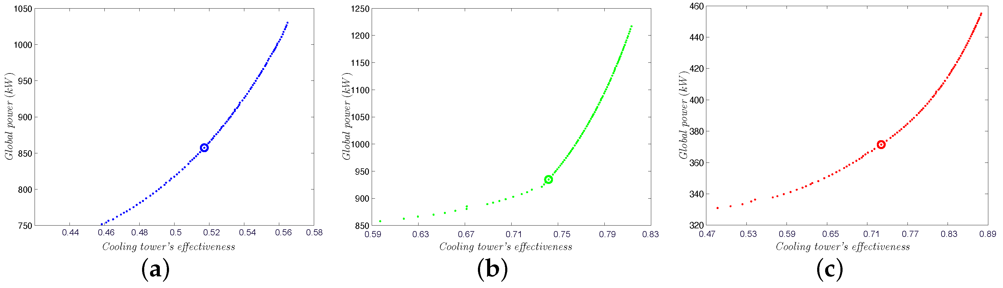
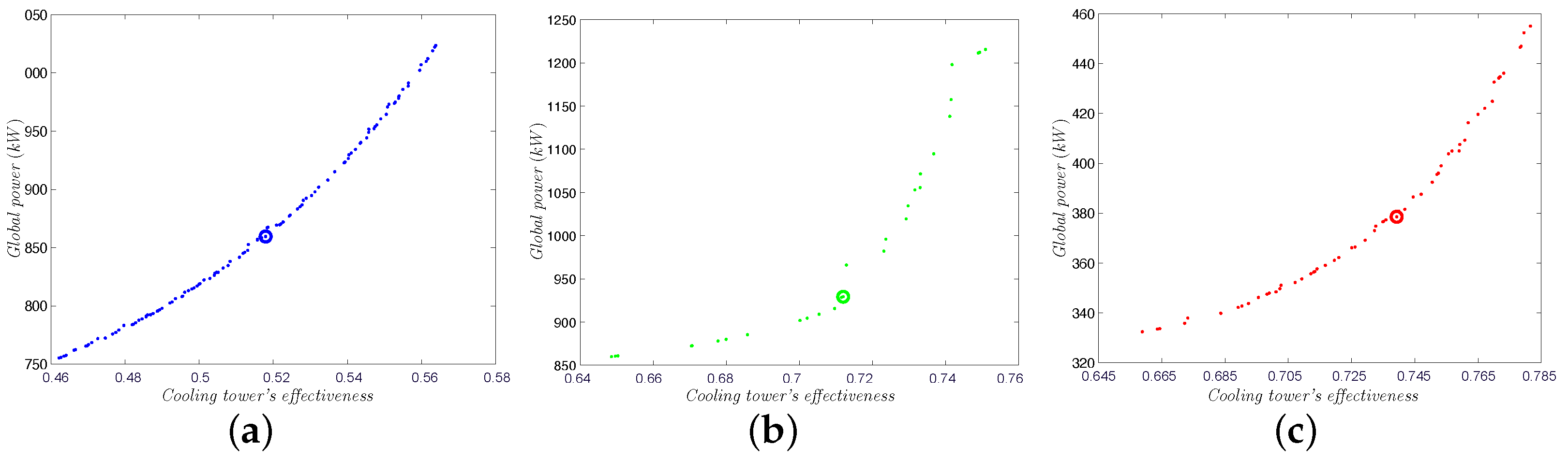
6.3. Preferred Solution Selection

Multi-objective algorithms return a set of solutions that guarantee a good trade-off between the optimization conflicting objectives. Therefore, we need a criterion to identify the adequate solutions to be applied in the real application at hand. There are several possible selection criteria [41]. In this work, we select the solution in the Pareto front that provides the lowest mean square of the normalized objectives.

In this application, the overall power consumption of the refrigeration system is in the order of hundreds of thousands of Watts while the effectiveness of the cooling tower varies between 0 and 1. Thus, the objective values must be normalized to avoid giving preference to solutions on the Pareto front that minimize the power consumption over those that maximize effectiveness. For this purpose, we normalize the system’s effectiveness metric using Equation (11) and to normalize the power consumption values, we apply Equation (12):

$${ϵ}_n=\frac{{ϵ}_e-{ϵ}_{min}}{{ϵ}_{max}-{ϵ}_{min}},$$

(11)

$$P_n=\frac{P_g-P_{min}}{P_{max}-P_{min}},$$

(12)

wherein ${ϵ}_n$ stands for the normalized effectiveness, ${ϵ}_{min}$ and ${ϵ}_{max}$ for the minimum and maximum effectiveness, respectively, considering all the Pareto front solutions. Likewise, $P_n$ stands for the normalized overall power consumption, and $P_{min}$ and $P_{max}$ for the minimum and maximum powers, respectively, considering all the Pareto front solutions.

Recall that the energy efficiency of the application, as modeled in this work, consists of maximizing the system’s effectiveness while minimizing its power consumption. So, the criterion defined for choosing the optimal solution is defined formally as in Equation (13):

$$S^{*}=\underset{F}{min}\left(\sqrt{\frac{0.5}{{ϵ}_n^2}+0.5P_n^2}\right),$$

(13)

wherein $S^{*}$ represents the solution selected from the Pareto front F. In this work, we consider that the two defined objectives are equally important to achieve the system’s energy efficiency. So, both objectives have the same weight.

In Figure 2, we show that the minimum point of the mean square curve of the normalized objectives can be used as a separator between the regions that favor one objective over the other. The solutions towards the left of the minimum point of this curve give preference to maximizing the system’s effectiveness, which is achieved by increasing the system’s power requirements. On the other side, the solutions towards the right of the minimum point of this curve give preference for minimizing the system’s power requirements, which is achieved by decreasing effectiveness, i.e., increasing its inverse $1/{ϵ}_a$.

The data used to evaluate the performance of applied optimization algorithms were collected in the field using the existing Supervisory Control and Data Acquisition (SCADA). The dataset includes 21,385 operational points at a rate of 1 point every 5 s. So the overall dataset was collected over 29 h and 42 min of operation of different days and times, so that we could contemplate different conditions of thermal load and different weather conditions. It is noteworthy to mention that the wet bulb temperatures were obtained from the database of the Instituto Nacional de Pesquisas Espaciais (INPE), available at [42], as recorded by the meteorological station at Santos Dummont airport in Rio de Janeiro/Brazil.

For the sake of synthesis and without loss of generality, the analysis presented in the sequel considers the results and Pareto fronts obtained by the applied algorithms, only for 3 points, namely 8, 16 and 26, of the 35 operational points of the whole dataset [43]. These points depict very different load situations.

Table 3. Collected data for the operational points used to discuss the performance of the optimization process.

Point	#Chillers	${\dot{\mathit{m}}}_{{\mathit{water}}_{\mathit{in}}}$ (kg/s)	${\mathit{T}}_{{\mathit{water}}_{\mathit{in}}}$ (°C)	${\mathit{T}}_{\mathit{BU}}$ (°C)	${\dot{\mathit{m}}}_{{\mathit{water}}_{\mathit{ev}}}$ (kg/s)	${\mathit{T}}_{{\mathit{ae}}_{\mathit{ev}}}$ (°C)	${\mathit{T}}_{{\mathit{as}}_{\mathit{ev}}}$ (°C)
8	2	87.02	29.68	22.94	130.53	10.41	6.01
16	2	70.71	29.40	24.49	106.07	11.16	6.27
26	1	51.65	27.94	23.31	154.96	9.72	6.05

presents the data for the illustrative operational points. During the period of time in which the field data are collected, a maximum of two chillers are used. Note that this does not impact the evaluation conducted herein, since the dataset includes 21,385 points, and was also used to validate the tower’s and chiller’s mathematical models [13,14].

6.4. SPEA2’s Performance Results

For the SPEA2 algorithm, the combined MATLAB/C++ implementation available in [44] is used. The parameters’ settings used are as follows: population equal to 100, probability of recombination equal to 5% and probability of mutation equal to 15%. In addition, the tournament is used for selecting the best individuals. The choice of these parameters was validated experimentally after repeated tests with several possible sets of parameters. We could verify that populations greater than 100 and recombination and mutation rates above the mentioned values only increased the execution time of the algorithm, not providing significant changes in the results nor in the quality of the obtained Pareto frontiers.

Table 4. Optimal solutions obtained by SPEA2 for the 4 operational points.

Point	SPEA2—50 Iterations					SPEA2—90 s
	${\mathit{n}}_{\mathit{best}}$ (Hz)	${\mathit{T}}_{\mathit{best}}$ (°C)	${\mathit{ϵ}}_{\mathit{a}}$	${\mathit{P}}_{\mathit{global}}$ (kW)	ec (%)	${\mathit{n}}_{\mathit{best}}$ (Hz)	${\mathit{T}}_{\mathit{best}}$ (°C)	${\mathit{ϵ}}_{\mathit{a}}$	${\mathit{P}}_{\mathit{global}}$ (kW)	ec (%)
8	44.28	6.27	0.5192	857.44	9.55	43.48	6.25	0.5178	858.30	9.45
16	60.00	6.91	0.7452	934.74	11.34	59.97	6.91	0.7451	935.46	11.27
26	58.22	6.80	0.7359	371.46	16.03	59.23	6.83	0.7402	372.43	15.79

presents the selected solutions, as evolved by SPEA2, together with the corresponding values of the objective functions for the 3 operational points (the results for all the 35 operational points used in the optimization are available in Appendix A of [43]). In this table, $n_{best}$ stands for the solution, ${ϵ}_a$ the effectiveness of the cooling tower, $P_g$ the global power required by fans and chillers and $ec$ the savings in terms of energy consumption.

Table 5. Verification of compliance of SPEA2 with the operational restrictions of the equipment for the 3 operational points.

Point	SPEA2—50 Iterations					SPEA2—90 s
	${\mathit{n}}_{\mathit{best}}$ (Hz)	${\mathit{T}}_{\mathit{best}}$ (°C)	${\mathit{T}}_{{\mathit{ae}}_{\mathit{co}}}$ (°C)	$\Delta \mathit{T}$ (°C)	${\mathit{T}}_{{\mathit{as}}_{\mathit{co}}}$ (°C)	${\mathit{n}}_{\mathit{best}}$ (Hz)	${\mathit{T}}_{\mathit{best}}$ (°C)	${\mathit{T}}_{{\mathit{ae}}_{\mathit{co}}}$ (°C)	$\Delta \mathit{T}$ (°C)	${\mathit{T}}_{{\mathit{as}}_{\mathit{co}}}$ (°C)
8	44.28	6.27	26.18	3.24	30.91	43.48	6.25	26.19	3.25	30.94
16	60.00	6.91	25.74	1.25	31.80	59.97	6.91	25.74	1.25	31.81
26	58.22	6.80	24.53	1.22	28.71	59.23	6.83	24.51	1.20	28.68

exhibits the parameters of the optimal solutions obtained that guarantee the established restrictions for the 3 operational points (the results for all the 35 operational points used in the optimization are available in Appendix B of [43]). As before, $T_{a{e}_{co}}$ stands for the predicted temperature for the water of the condenser circuit that leaves the cooling tower and travels towards the chillers, and $T_{a{s}_{co}}$ the predicted temperature for the water in the condenser circuit, that leaves the chillers and goes towards the cooling tower.

Comparing the results obtained with the two stopping criteria, i.e., after 50 iterations and after 90 s, we verify that after a number of iterations greater than 50, operational points 8 and 16 converge to solutions that provide a reduction in both savings and in the effectiveness of the tower, compared to the result obtained for 50 iterations. This is due to the fact that the algorithm’s execution with stopping criterion after 90 s is not a continuation of that after 50 iterations, i.e., these are different executions, and due to the stochastic character of the algorithm, it cannot be guaranteed that the solutions obtained in different executions are identical, but rather they represent very close points. Points 8 and 16 show reductions in global energy savings of 0.1% and 0.07%, respectively, and reductions in effectiveness of 0.14% and 0.01%, respectively, after new executions with a number of iterations greater than 50. We observe that this does not rule out the optimal solutions presented for these points, since they ensure a good trade-off between the established objectives. The variations in the achieved results for the different stopping criteria are negligible in practical terms.

Operational point 26, after execution with a number of iterations greater than 50, shows a reduction of 0.24% in global energy savings, in order to obtain an increase of 0.43% in the tower’s effectiveness.

Figure 3 shows the Pareto front obtained for the stopping condition of 50 iterations for the 3 operational points indicated in Table 4 and Table 5. Figure 4 shows the Pareto front obtained for the stopping conditions of 90 s for the 3 operational points indicated in Table 4 and Table 5. In both fronts, the circled points represent the chosen optimal solution. Note that the Pareto fronts obtained when using both stopping conditions are identical, verifying the correct convergence of the algorithm.

6.5. NSGA-II’s Performance Results

For the NSGA-II algorithm, the MATLAB implementation available in [45] is used. The parameters’ settings used are as follows: population equal to 100, probability of recombination equal to 0.8 and probability of mutation equal to 0.3. In addition, the binary tournament is used to select the best individuals. Once again, the parameter values are chosen based on tests carried out in order to reduce the execution time and obtain a Pareto front with good distribution and sufficient number of solutions.

Table 6. Optimal solutions obtained by NSGA-II for the 4 operational points.

Point	NSGA-II—50 Iterations					NSGA-II—90 s
	${\mathit{n}}_{\mathit{best}}$ (Hz)	${\mathit{T}}_{\mathit{best}}$ (°C)	${\mathit{ϵ}}_{\mathit{a}}$	${\mathit{P}}_{\mathit{global}}$ (kW)	$\mathit{ec}$ (%)	${\mathit{n}}_{\mathit{best}}$ (Hz)	${\mathit{T}}_{\mathit{best}}$ (°C)	${\mathit{ϵ}}_{\mathit{a}}$	${\mathit{P}}_{\mathit{global}}$ (kW)	$\mathit{ec}$ (%)
8	44.46	6.26	0.5196	859.03	9.37	46.04	6.28	0.5223	859.98	9.26
16	59.88	6.95	0.7448	928.58	11.96	59.78	6.93	0.7444	930.36	11.78
26	56.87	6.71	0.7301	372.54	15.76	57.37	6.73	0.7323	373.09	15.62

presents the selected solutions, as evolved by NSGA-II, together with the corresponding values of the objective functions for the 3 operational points (the results for all the 35 operational points used in the optimization are available in Appendix A of [43]). In this table, $n_{best}$ stands for the solution, ${ϵ}_a$ the effectiveness of the cooling tower, $P_g$ the global power required by fans and chillers and $ec$ the savings in terms of energy consumption.

Table 7. Verification of compliance of NSGA-II with the operational restrictions of the equipment for the 3 operational points.

Point	NSGA-II—50 Iterations					NSGA-II—90 s
	${\mathit{n}}_{\mathit{best}}$ (Hz)	${\mathit{T}}_{\mathit{best}}$ (°C)	${\mathit{T}}_{{\mathit{ae}}_{\mathit{co}}}$ (°C)	$\Delta \mathit{T}$ (°C)	${\mathit{T}}_{{\mathit{as}}_{\mathit{co}}}$ (°C)	${\mathit{n}}_{\mathit{best}}$ (Hz)	${\mathit{T}}_{\mathit{best}}$ (°C)	${\mathit{T}}_{{\mathit{ae}}_{\mathit{co}}}$ (°C)	$\Delta \mathit{T}$ (°C)	${\mathit{T}}_{{\mathit{as}}_{\mathit{co}}}$ (°C)
8	44.46	6.26	26.18	3.24	30.92	46.04	6.28	26.16	3.22	30.89
16	59.88	6.95	25.74	1.25	31.76	59.78	6.93	25.74	1.25	31.78
26	56.87	6.71	24.56	1.25	28.79	57.37	6.73	24.55	1.24	28.78

exhibits the parameters of the optimal solutions obtained that guarantee the established restrictions for the 3 operational points (the results for all the 35 operational points used in the optimization are available in Appendix B of [43]). Recall that $T_{a{e}_{co}}$ stands for the predicted temperature for the water of the condenser circuit that leaves the cooling tower and travels towards the chillers, and $T_{a{s}_{co}}$ the predicted temperature for the water in the condenser circuit that leaves the chillers and goes towards the cooling tower.

Comparing the results obtained for the stopping criteria after 50 iterations and after 90 s, it appears that, after a number of iterations greater than 50, for the operational points, indicated in Table 6, the optimization converged to solutions that reduce the overall energy savings while achieving a better or similar value for tower effectiveness. In this case, the optimization regarding operating point 8 presents a reduction of 0.11% in energy savings for an increase of 0.27% in the effectiveness of the tower. The optimization regarding point 26 shows a 0.14% reduction in overall energy savings for a 0.22% increase in effectiveness. Unlike the others, for point 16 the optimization exhibits a reduction in both consumption and effectiveness, respectively, of 0.18% and 0.04%, and this is due to the fact that the execution with stopping criterion of 90 s is not a continuation of that of 50 iterations. As noted before, for the stochastic character of the algorithms, it cannot be guaranteed that they will converge to exactly the same solution, but rather to very close points.

Figure 5 shows the Pareto front obtained when using the stopping condition of 50 iterations for the 3 operational points indicated in Table 6 and Table 7. Figure 6 presents the Pareto front achieved for the stopping criterion of 90 s for the 3 operational points indicated in Table 6 and Table 7. The circled points represent the selected optimal solution. Note that the Pareto fronts obtained for the two stopping criteria are practically identical, verifying the proper convergence of the algorithm.

6.6. Micro-GA’s Performance Results

For the Micro-GA algorithm, the Toolbox SGALAB from MATLAB [46] is used. The parameters’ settings used are as follows: population memory equal to 100, external memory equal to 100, percentage of non-replaceable memory equal to 20%, internal Micro-GA population equal to 6, recombination rate equal to 0.8, mutation rate equal to 0.2, number of Micro-GA iterations until achieving nominal convergence equal to 4 and a replacement cycle of 15 iterations. The binary tournament is used for selecting the best individuals. These values are obtained based on the recommended values in [21] and through experiments in order to obtain a Pareto boundary with good distribution with a fast possible convergence. It is noteworthy to point out that higher values for the mutation rate and for the initial population only increased the algorithm convergence time, leaving the results practically unchanged. Differently from what is indicated in [21], where it is suggested that values for the internal population should be set as 3 to 4, we notice, in this case, that the use of an internal population equal to 6 allowed us to further reduce the algorithm convergence time.

Table 8. Optimal solutions obtained by Micro-GA for the 4 operational points.

Point	Micro-GA—50 Iterations					Micro-GA—90 s
	${\mathit{n}}_{\mathit{best}}$ (Hz)	${\mathit{T}}_{\mathit{best}}$ (°C)	${\mathit{ϵ}}_{\mathit{a}}$	${\mathit{P}}_{\mathit{global}}$ (kW)	$\mathit{ec}$ (%)	${\mathit{n}}_{\mathit{best}}$ (Hz)	${\mathit{T}}_{\mathit{best}}$ (°C)	${\mathit{ϵ}}_{\mathit{a}}$	${\mathit{P}}_{\mathit{global}}$ (kW)	$\mathit{ec}$ (%)
8	43.50	6.26	0.5179	857.17	9.58	43.54	6.20	0.5179	865.90	8.58
16	56.67	6.77	0.7322	946.05	10.21	53.24	6.81	0.7181	929.14	11.90
26	57.29	6.74	0.7320	372.23	15.83	58.30	6.65	0.7363	378.59	14.27

presents the selected solutions, as evolved by Micro-GA, together with the corresponding values of the objective functions for the 3 operational point s(The results for all the 35 operational points used in the optimization are available in Appendix A of [43]). In this table, $n_{best}$ stands for the solution, ${ϵ}_a$ the effectiveness of the cooling tower, $P_g$ the global power required by fans and chillers and $ec$ the savings in terms of energy consumption.

Table 9. Verification of compliance of Micro-GA with the operational restrictions of the equipment for the 3 operational points.

Point	Micro-GA—50 Iterations					Micro-GA—90 s
	${\mathit{n}}_{\mathit{best}}$ (Hz)	${\mathit{T}}_{\mathit{best}}$ (°C)	${\mathit{T}}_{{\mathit{ae}}_{\mathit{co}}}$ (°C)	$\Delta \mathit{T}$ (°C)	${\mathit{T}}_{\mathit{a}{\mathit{s}}_{\mathit{c}\mathit{o}}}$ (°C)	${\mathit{n}}_{\mathit{best}}$ (Hz)	${\mathit{T}}_{\mathit{best}}$ (°C)	${\mathit{T}}_{{\mathit{ae}}_{\mathit{co}}}$ (°C)	$\Delta \mathit{T}$ (°C)	${\mathit{T}}_{{\mathit{as}}_{\mathit{co}}}$ (°C)
8	43.50	6.26	26.19	3.25	30.93	43.54	6.20	26.19	3.25	30.98
16	56.67	6.77	25.81	1.32	32.03	53.24	6.81	25.87	1.38	32.05
26	57.29	6.74	24.55	1.24	28.77	58.30	6.65	24.53	1.22	28.80

exhibits the parameters of the optimal solutions obtained that guarantee the established restrictions for the 3 operational points (the results for all the 35 operational points used in the optimization are available in Appendix B of [43]). As before, $T_{a{e}_{co}}$ stands for the predicted temperature for the water of the condenser circuit that leaves the cooling tower and travels towards the chillers, and $T_{a{s}_{co}}$ the predicted temperature for the water in the condenser circuit that leaves the chillers and goes towards the cooling tower.

Comparing the results obtained after executing the Micro-GA with different stopping criteria, i.e., after 50 iterations and after 90 s, we note that the optimization regarding operating point 8 offered the same effectiveness for both criteria, varying only in the achieved global energy savings. After 90 s, a reduction of 1.00% is achieved. Recall that the different stopping criteria occasion different executions, and due to the stochastic character of the optimization algorithms, there could be a deviation between the results. Nonetheless, a convergence confirmation of the algorithm regarding the region containing the optimal solutions is apparent. The optimization regrading operational point 16 shows a reduction of 1.41% in the tower’s effectiveness in order to obtain a 1.72% increase in global energy savings. For point 26, the optimization reaches a reduction of 1.58% in the overall energy savings in order to obtain an increase of 0.43% in the tower’s effectiveness.

As observed for operational points 26, the result obtained after 90 s is below that obtained after 50 iterations, since the reduction in energy savings is lower than the increase in effectiveness in the tower. This is due to the fact that the criterion for choosing the optimal solution adopted does not verify whether the new optimal solution obtained in a new execution is better or worse than the one obtained in the previous optimization, with 50 iterations. The stopping criteria are applied in two different executions of the algorithm. Thus, after reaching the stopping criterion, the optimal point is simply chosen based on the lowest mean square of the normalized objectives, without evaluating whether the result obtained with the stopping criterion after 90 s is better or worse than after 50 iterations. In this work, the comparison between the optimal solutions obtained for each stopping criterion is performed in a stage after the execution of the algorithm.

Figure 7 presents the Pareto fronts obtained for the stopping criterion of 50 iterations for the 3 operational points indicated in Table 8 and Table 9. Figure 8 shows the Pareto fronts obtained for the stopping criterion of 90 s for the 3 operational points indicated in Table 8 and Table 9. The circled points represent the preferred optimal solution. Note that the reached Pareto fronts do not have satisfactory solution distribution, as was the case for SPEA2 and NSGA-II. It can also be observed that there is a visible displacement in the optimal solutions obtained after 90 s, which is not satisfactory. Even so, the obtained results confirm the convergence of the algorithm, since the variations verified for the objectives are very small and the solutions for the two stopping criteria are very close.

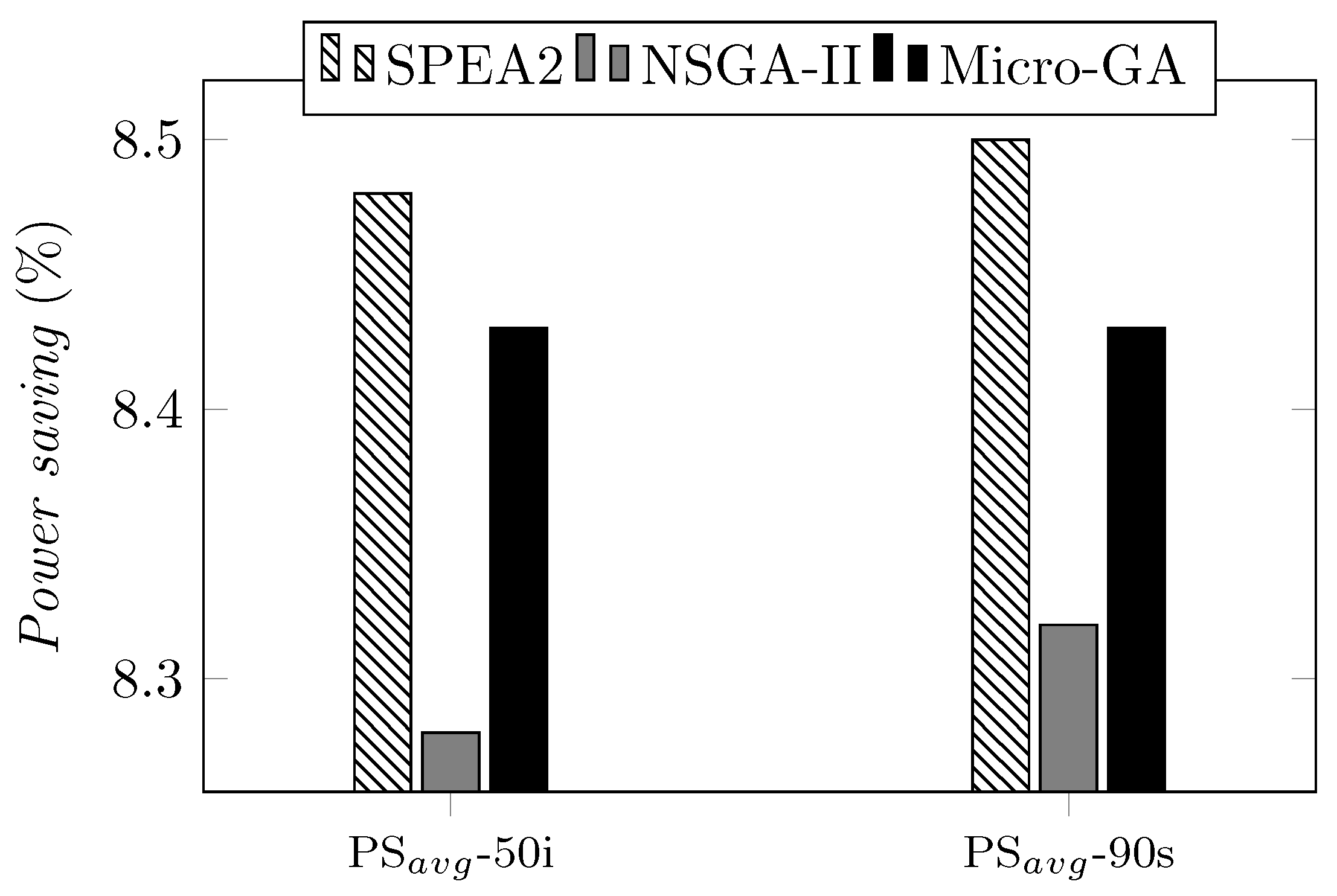
7. Performance Comparison

We now compare the results obtained by the optimization processes when using multi-objective algorithms SPEA2, NSGA-II and Micro-GA. First of all, the obtained results are compared to collected field data to evaluate the gains obtained in terms of energy savings and cooling tower effectiveness. Then, the results achieved by the algorithms are compared with each other in order to choose the most adequate algorithm for the application. Three metrics are used in the comparison and selection process:

• The average, minimum and maximum savings obtained in terms of power consumption by the refrigeration system;
• The average, minimum and maximum effectiveness reached for the cooling tower;
• The ratio between the average savings in terms of overall power consumption and the corresponding reduction in terms of average effectiveness of the cooling tower;

where the average values are computed by applying the optimization results to the 21,385 collected field data regarding the 35 operational points. In this work, the third metric will be termed Energy Efficiency Ratio (EER). It is computed using Equation (14):

$$\mathrm{EER}=\frac{{\mathrm{PS}}_{avg}}{\Delta {ϵ}_{avg}}$$

(14)

Table 10. Metrics evaluation for the three applied algorithms regarding both stopping criteria.

Metric	After 50 Iterations			After 90 s
	SPEA2	NSGA-II	Micro-GA	SPEA2	NSGA-II	Micro-GA
$P{S}_{avg}$ (%)	8.48	8.28	8.43	8.50	8.32	8.43
$P{S}_{min}$ (%)	−3.72	−4.09	−4.64	−3.72	−4.26	−3.66
$P{S}_{max}$ (%)	26.07	25.36	25.67	25.27	26.16	25.46
${ϵ}_{avg}$	0.6232	0.6219	0.6183	0.6247	0.6200	0.6159
${ϵ}_{min}$	0.4843	0.4826	0.4818	0.4833	0.4818	0.4816
${ϵ}_{max}$	0.8474	0.8470	0.8350	0.8473	0.8466	0.8285
Time (s)	15.70	69.82	77.92	90	90	90
#Iterations	50	50	50	548	63	78

presents the evaluated metrics results of SPEA2, NSGA-II and Micro-GA, regarding both stopping criteria. The values indicated refer to the application of the results obtained for the 35 operational points as presented in Appendix A of [43] to the 21,385 actual field data collected from the real refrigeration system. The execution time indicates the average time spent by the implementation of the considered algorithm with the stopping criterion of 50 iterations. This time duration is given in seconds. For the 90 s case, we report the number of required iterations instead, as the execution time is fixed, i.e., 90 s.

In Table 10, we can observe that the algorithms implemented in MATLAB (NSGA-II and Micro-GA) require a longer execution time for 50 iterations compared to algorithms implemented in C++ (SPEA2). This result is expected. However, it is noteworthy that the execution time in a dedicated implementation for real usage purposes will depend on the characteristics of the running processor and available memory resources. Moreover, a more efficient codification of the selected algorithm can always be achieved. For both stopping criteria, we can also observe that the algorithm that achieved the best average power savings is SPEA2 followed Micro-GA by NSGA-II. Figure 9 allows a visual comparison of the improvement yielded in terms of average power savings for both stopping criteria (PS_avg—50 i; and PS_avg—90 s). It is noteworthy to point out that SPEA2 provides a solution that offers a greater average power saving in the case of the 90 s based stopping criterion.

Moreover, note that for both stopping criteria, SPEA2 presents the best average effectiveness, but in this case followed by NSGA-II then Micro-GA. For the first stopping criterion, the optimization time for SPEA2 is the lowest but in the case of the second stopping criterion, the number of iterations required by SPEA2 is the highest. Notably, there are records of negative values of power energy savings, which occur at points wherein the fan speed in the field collected data is 30 Hz. In these cases, the optimization also suggests increasing their speed in order to increase the tower’s effectiveness, with a consequent increase in the power energy consumption of the system. This is consistent and matches the expected solution for the proposed optimization system. Figure 10 allows a visual comparison of the improvement yielded in terms of average effectiveness of the tower for both applied algorithms for both stopping criteria (${ϵ}_{avg}$—50 i; and ${ϵ}_{avg}$—90 s). Once again, it is noteworthy to point out that SPEA2 provides a solution that offers a greater average cooling tower effectiveness in the case of the 90 s based stopping criterion.

It is known that the system’s effectiveness depends not only on the setpoints of the cooling tower operation, but also on external factors, such as ambient temperature and wet bulb temperature. Thus, the reference value for evaluating the algorithms must be at least the average effectiveness obtained by applying the 21,385 operational points collected for the cooling tower modeling, which is 0.6761. Hence, the best algorithm for the application must be the one that achieves the highest average global power savings, with the least possible detriment to the average effectiveness of the cooling tower.

It is noteworthy to point out that, in

Table 11. Results for the selection of the best algorithm considering both stopping criteria.

Metric	After 50 Iterations			After 90 s
	SPEA2	NSGA-II	Micro-GA	SPEA2	NSGA-II	Micro-GA
$P{S}_{avg}$ (%)	8.48	8.28	8.43	8.50	8.32	8.43
${ϵ}_{avg}$ (%)	62.32	62.19	61.83	62.47	62.00	61.59
$\Delta {ϵ}_{avg}$ (%)	5.29	5.42	5.78	5.14	5.61	6.02
EER	1.60	1.53	1.46	1.65	1.48	1.40

, for all three algorithms, the value of EER is greater than 1, which is quite satisfactory. This means that the power savings achieved outweigh the reduction in effectiveness of the cooling tower. So, for both stopping criteria, we note that we have In decreasing order of performance: SPEA2, NSGA-II then Micro-GA. SPEA2 offers the highest value of EFR, which corresponds to 1.60 and 1.65, respectively. So, for the second stopping criterion, SPEA2 achieves a power savings of about to 1.65 times the reduction in the tower effectiveness.

A reduction in the performance of the NSGA-II and Micro-GA algorithms can be seen when comparing the values of $FER$ obtained with the stopping criteria after 50 iterations and after 90 s. For NSGA-II, this factor reduces from 1.53 to 1.48, and for Micro-GA, from 1.46 to 1.40. This is mainly due to the criterion used to choose the optimal solution, which is impacted by the Pareto front distribution. In this case, after 90 s, NSGA-II and Micro-GA added points to the Pareto front that led the adopted decision criterion to choose optimal solutions that favored an increase in terms of average effectiveness of the cooling tower. Figure 11 allows a visual comparison of the improvement yielded in terms of average effectiveness of the tower for both applied algorithms for both stopping criteria (${ϵ}_{avg}$—50 i; and ${ϵ}_{avg}$—90 s). Note that, as expected, the solution provided by SPEA2 offers a greater energy efficiency ration in the case of the 90 s based stopping criterion.

So, it is now safe to conclude that SPEA2 is the best algorithm for the studied application and that the 90 s based stopping criterion is more adequate as it allows for a more interesting trade-off between average power saving and average tower effectiveness, yielding a better ration regarding energy efficiency.

8. Conclusions

The proposed work analyzes the feasibility of applying a multi-objective optimization to the operation of refrigeration systems based on cooling towers and chillers, in order to obtain the operational setpoints that meet the best compromise between two conflicting objectives: reduction of energy consumption and increasing of the tower’s effectiveness. This allows obtaining the maximum energy efficiency possible for the whole refrigeration system. For this purpose, it is necessary to formally model the main equipment involved in the considered refrigeration system. Precise and faithful models for the cooling towers and its fans and for the chiller have been developed previously. We also conducted a preliminary survey to select evolutionary multi-objective optimization algorithms to be applied. Algorithms SPEA2, NSGA-II and Micro-GA are chosen so as to investigate their performance regarding the energy efficiency optimization.

We conducted a thorough analysis of the Pareto fronts yielded by the usage of the chosen algorithms. This is performed based on two optimization scenarios with regards to the stopping criterion to be used: either a fixed number of iterations (50 iterations) or a fixed time interval (90 s). We considered these two possibilities so as to obtain the optimal solution to be applied to the real refrigeration system, hence yielding the expected energy efficiency. These iteration and time thresholds are thus set to meet the requirements of the application and to verify the performance impact of the solution reached by the optimization process. After analyzing the obtained global performance results, we conclude that the results obtained with SPEA2 when combined with the stopping criterion of after 90 s should be adopted.

There are several directions to carry on this work aiming at improving the analysis. The used models can be made more sophisticated to offer support for other kind of chillers. In addition, it would be interesting to compare the performance of the chosen algorithms by varying the speed of the condensed and chilled water pumps. The frequency converters could be considered in the optimization process. In this case, the variation of the speed of the cooling tower’s fans would have to be taken into account. Furthermore, in the present work, the increase in terms of water consumption of the refrigeration system is not considered in contrast to the reduction of the cooling tower’s effectiveness. Thus, developing a model that estimates the system’s water consumption in terms of the tower’s effectiveness would be interesting. There is also the possibility to explore the usage of other kinds of multi-objective optimization algorithms, such as those based on swarming strategies as apposed to the evolutionary strategy. Among these algorithms, we can mention the work in progress exploring multi-objective particle swarm optimization and multi-objective tribe optimization. Another possible direction could be the study of the effects of cryogenic fluids on the system’s energy efficiency.

References

1. Dondapati, R.S.; Saini, V.; Verma, K.N.; Usurumarti, P.R. Computational prediction of pressure drop and heat transfer with cryogen based nanofluids to be used in micro-heat exchangers. Int. J. Mech. Sci. 2017, 130, 133–142. [Google Scholar] [CrossRef]
2. Dondapati, R.S.; Rao, V. Entropy generation minimization (EGM) to optimize mass flow rate in dual channel cable-in-conduit conductors (CICCs) used for fusion grade magnets. Fusion Eng. Des. 2014, 89, 837–846. [Google Scholar] [CrossRef]
3. Chakravarthy, V.; Shah, R.; Venkatarathnam, G. A Review of Refrigeration Methods in the Temperature Range 4–300 K. J. Therm. Sci. Eng. Appl. 2011, 3, 020801. [Google Scholar] [CrossRef]
4. Yu, K.; Hung, Y.; Hsieh, S.; Hung, S. Chiller Energy Saving Optimization Using Artificial Neural Networks. J. Appl. Sci. 2011, 16, 3008–3014. [Google Scholar] [CrossRef] [Green Version]
5. Pegallapati, A.S.; Ramgopal, M. Effect of heat transfer area distribution on frosting performance of refrigerator evaporator. Int. J. Heat Mass Transf. 2021, 175, 121317. [Google Scholar] [CrossRef]
6. Li, X.; Li, Y.; Seem, J.E.; Li, P. Extremum seeking control of cooling tower for self-optimizing efficient operation of chilled water systems. In Proceedings of the 2012 American Control Conference, Montreal, QC, Canada, 27–29 June 2012; pp. 3396–3401. [Google Scholar] [CrossRef]
7. Tyagi, V.; Sane, H.; Darbha, S. An extremum seeking algorithm for determining the set point temperature for condensed water in a cooling tower. In Proceedings of the 2006 American Control Conference, Minneapolis, MN, USA, 14–16 June 2006; pp. 1127–1131. [Google Scholar] [CrossRef]
8. Liu, C.; Chuah, Y. A study on an optimal approach temperature control strategy of condensing water temperature for energy saving. Int. J. Refrig. 2011, 34, 816–823. [Google Scholar] [CrossRef]
9. Ma, Z.; Wang, S. Supervisory and optimal control of central chiller plants using simplified adaptive models and genetic algorithm. Appl. Energy 2011, 88, 198–211. [Google Scholar] [CrossRef]
10. Kie, P.L.T.; Theng, L. Intelligent Control of Heating, Ventilating and Air Conditioning Systems. In Advances in Neuro-Information Processing; Lecture Notes in Computer Science; Springer: Heidelberg/Berlin, Germany, 2009; Volume 5507, pp. 927–934. [Google Scholar]
11. Singh, K.; Das, R. Simultaneous optimization of performance parameters and energy consumption in induced draft cooling towers. Chem. Eng. Res. Des. 2017, 123, 1–13. [Google Scholar] [CrossRef]
12. Jia, L.; Wei, S.; Liu, J. A review of optimization approaches for controlling water-cooled central cooling systems. Build. Environ. 2021, 203, 108100. [Google Scholar] [CrossRef]
13. Nedjah, N.; Mourelle, L.M.; Lizarazu, M.S.D. Mathematical Modeling of Cooling Tower-based Refrigeration Systems for Energy Efficiency Optimization. In Proceedings of the International Conference on Computational Science and Its Applications, Malaga, Spain, 4–7 July 2022. [Google Scholar]
14. Nedjah, N.; Mourelle, L.M.; Lizarazu, M.S.D. Mathematical Modeling of Chiller-based Refrigeration Systems for Energy Efficiency Optimization. In Proceedings of the International Conference on Computational Science and Its Applications, Malaga, Spain, 4–7 July 2022. [Google Scholar]
15. More, J.J. The Levenberg–Marquardt algorithm: Implementation and theory. Numer. Anal. 1978, 630, 105–116. [Google Scholar]
16. YORK. Curva de Surge das Unidades Resfriadoras UR-S2O3, UR-S2O4, UR-S2O5 e RU-S2O6; Technical Report; YORK: Sorocaba, SP, Brazil, 2009. [Google Scholar]
17. Alpina. Memória de cálculo das torres de resfriamento TR-2501 e TR-2502; Technical Report; Alpina S/A Indústria e Comércio: São Bernardo do Campo, SP, Brazil, 2013. [Google Scholar]
18. Goldberg, D.E. Genetic Algorithms in Search, Optimization and Machine Learning. Addion Wesley 1989, 1989, 36. [Google Scholar]
19. Nedjah, N.; Mourelle, L.M. Real World Multi-Objective System Engineering; Intelligent System Engineering Series; Nova Science Publishers: New York, NY, USA, 2005. [Google Scholar]
20. Nedjah, N.; de Macedo Mourelle, L. Evolutionary multi-objective optimisation: A survey. Int. J. Bio Inspired Comput. 2015, 7, 1–25. [Google Scholar] [CrossRef]
21. Coello, C.A.C.; Pulido, G.T. A Micro-Genetic Algorithm for Multiobjective Optimization. In First International Conference on Evolutionary Multi-Criterion Optimization; Number 1993 in Lecture Notes in Computer Science; Springer: Zurich, Switzerland, 2001; pp. 126–140. [Google Scholar]
22. Srinivas, N.; Deb, K. Muiltiobjective Optimization Using Nondominated Sorting in Genetic Algorithms. Evol. Comput. 1994, 2, 221–248. [Google Scholar] [CrossRef]
23. Horn, J.; Nafpliotis, N.; Goldberg, D. A niched Pareto genetic algorithm for multiobjective optimization. In Proceedings of the First IEEE Conference on Evolutionary Computation, IEEE World Congress on Computational Intelligence, Orlando, FL, USA, 27–29 June 1994; Volume 1, pp. 82–87. [Google Scholar] [CrossRef]
24. Knowles, J.D.; Corne, D.W. Approximatting the Non-Dominated Front Using the Pareto Archived Evolution Strategy. Evol. Comput. J. 2000, 8, 149–172. [Google Scholar] [CrossRef] [PubMed]
25. Knowles, J.; Corne, D. M-PAES: A memetic algorithm for multiobjective optimization. In Proceedings of the 2000 Congress on Evolutionary Computation, CEC00 (Cat. No.00TH8512), La Jolla, CA, USA, 16–19 July 2000; Volume 1, pp. 325–332. [Google Scholar] [CrossRef]
26. Deb, K.; Agrawal, S.; Pratap, A.; Meyarivan, T. A Fast Elitist Non-dominated sorting genetic algorithm for multi-objective optimization: NSGA-II. In Proceedings of the Parallel Problem Solving from Nature VI Conference, Paris, France, 18–20 September 2000; Volume 1917, pp. 849–858. [Google Scholar]
27. Veldhuizen, D.A.V.; Lamont, G.B. Multiobjective Optimization with Messy Genetic Algorithms. In Proceedings of the 2000 Symposium on Applied Computing, Como, Italy, 19–21 March 2000; pp. 470–476. [Google Scholar] [CrossRef]
28. Laumanns, M.; Thiele, L.; Deb, K.; Zitzler, E. Combining Convergence and Diversity in Evolutionary Multi-objective Optimization. Evol. Comput. 2002, 10, 263–282. [Google Scholar] [CrossRef] [PubMed]
29. Zitzler, E.; Thiele, L. An Evolutionary Algorithm for Multiobjective Optimization: The Strength Pareto Approach; Technical Report 43; Computer Engineering and Communication Networks Lab (TIK), Swiss Federal Intitute of Technology (ETH): Zurich, Switzerland, 1998. [Google Scholar]
30. Rudolph, G. Evolutionary Search under Partially Ordered Sets; Tech. Rep. CI-67/99; Department of Computer Science/LS11, University of Dortmund: Dortmund, Germany, 1999. [Google Scholar]
31. Corne, D.; Knowles, J.; Oates, M. The Pareto Envelope-Based Selection Algorithm for Multi- Objective optimization. In Proceedings of the Sixth International Conference on Parallel Problem Solving from Nature, PPSN-VI, Paris, France, 18–20 September 2000; pp. 839–848. [Google Scholar]
32. Kim, M.; Hiroyasu, T.; Miki, M.; Watanabe, S. SPEA2+: Improving the Performance of the Strength Pareto Evolutionary Algorithm 2. In Proceedings of the International Conference on Parallel Problem Solving from Nature 2004, Birmingham, UK, 18–24 September 2004; pp. 742–751. [Google Scholar]
33. Guo, D.; Wang, J.; Huang, J.; Han, R.; Song, M. Chaotic-NSGA-II: An Effective Algorithm to Solve Multi-objective Problems. In Proceedings of the International Conference on Intelligent Computing and Integrated Systems (ICISS), Guilin, China, 22–24 October 2010; pp. 20–23. [Google Scholar] [CrossRef]
34. Li, M.; Yang, S.; Liu, X.; Wang, K. IPESA-II: Improved Pareto Envelope-Based Selection Algorithm II. Evol. Multi-Criterion Optim. Lect. Notes Comput. Sci. 2013, 7811, 143–155. [Google Scholar] [CrossRef]
35. Deb, K.; Jain, H. An evolutionary many-objective optimization algorithm using reference-point-based nondominated sorting approach, part I: Solving problems with box constraints. Evol. Comput. IEEE Trans. 2014, 18, 577–601. [Google Scholar] [CrossRef]
36. Sulieman, D.; Jourdan, L.; Talbi, E.G. Using multiobjective metaheuristics to solve VRP with uncertain demands. In Proceedings of the IEEE Congress on Evolutionary Computation, Barcelona, Spain, 18–23 July 2010; pp. 1–8. [Google Scholar] [CrossRef]
37. Zitzler, E.; Laumanns, M.; Thiele, L. SPEA2: Improving the Strength Pareto Evolutionary Algorithm; TIK-Report 103; Swiss Federal Institute of Technology: Zürich, Switzerland, 2001. [Google Scholar]
38. Deb, K. Multi-Objective Optimization Using Evolutionary Algorithms; Wiley and Sons: New York, NY, USA, 2001. [Google Scholar]
39. Goldberg, D.E. Sizing Populations for Serial and Parallel Genetic Algorithms. In Proceedings of the Third International Conference on Genetic Algorithms, Fairfax, WV, USA, 4–7 June 1989; Schaffer, J.D., Ed.; Morgan Kaufmann: San Mateo, CA, USA, 1989; pp. 70–79. [Google Scholar]
40. YORK. Print-out de seleção das Unidades Resfriadoras UR-S2O3, UR-S2O4, UR-S2O5 e UR-S2O6; Technical Report; YORK: Sorocaba, SP, Brazil, 2006. [Google Scholar]
41. Sayyaadi, H.; Nejatolahi, M. Multi-objective optimization of a cooling tower assisted vapor compression refrigeration system. Int. J. Refrig. 2011, 34, 243–256. [Google Scholar] [CrossRef]
42. INPE. Dados Observacionais do Centro de Previsão de Tempo e Estudos Climáticos. 2014. Available online: http://bancodedados.cptec.inpe.br (accessed on 26 June 2022).
43. Lizarazu, M.S.D. Otimização Multiobjetivo Aplicada à Efciência Energética de Torres de Resfriamento. Master’s Thesis, Universidade do Estado do Rio de Janeiro, Rio de Janeiro, Brazil, 1996. Available online: https://www.pel.uerj.br/bancodissertacoes/Dissertacao_Marcelo_Lizarazu.pdf (accessed on 26 June 2022).
44. Popov, A. Combined Matlab—C Implementation of SPEA2; MathWorks: Natick, MA, USA, 2007. [Google Scholar]
45. Heris, S.M.K. A Version of the NSGA-II in Matlab. 2010. Available online: http://delta.cs.cinvestav.mx/~ccoello/EMOO/EMOOsoftware.html (accessed on 26 June 2022).
46. Chen, L. SGALAB 1003 Beta 5.0.0.8 (Matrix Variable Inputs): Genetic Algorithm Toolbox for Multi-objective Problems with Fuzzy Logic Controller Applications; MathWorks: Natick, MA, USA, 2004. [Google Scholar]
Figure 1. Refrigeration system’s configuration.
Energies 15 05575 g001
Figure 2. Illustration used to motivate the usage of the selection criterion of the best solution.
Energies 15 05575 g002
Figure 3. Pareto fronts and selected optimal solutions for 3 of the 35 operating points used in the implementation of the optimization with SPEA2 with stopping criterion after 50 iterations. (a) Operational point 8; (b) Operational point 16; (c) Operational point 26.
Energies 15 05575 g003
Figure 4. Pareto fronts and selected optimal solutions for 3 of the 35 operating points used in the implementation of the optimization with SPEA2 with stopping criterion after 90 s. (a) Operational point 8; (b) Operational point 16; (c) Operational point 26.
Energies 15 05575 g004
Figure 5. Pareto fronts and selected optimal solutions for 3 of the 35 operating points used in the implementation of the optimization with NSGA-II with stopping criterion after 50 iterations. (a) Operational point 8; (b) Operational point 16; (c) Operational point 26.
Energies 15 05575 g005
Figure 6. Pareto fronts and selected optimal solutions for 3 of the 35 operating points used in the implementation of the optimization with NSGA-II with stopping criterion after 90 s. (a) Operational point 8; (b) Operational point 16; (c) Operational point 26.
Energies 15 05575 g006
Figure 7. Pareto fronts and selected optimal solutions for 3 of the 35 operating points used in the implementation of the optimization with Micro-GA with stopping criterion after 50 iterations. (a) Operational point 8; (b) Operational point 16; (c) Operational point 26.
Energies 15 05575 g007
Figure 8. Pareto fronts and selected optimal solutions for 3 of the 35 operating points used in the implementation of the optimization with Micro-GA with stopping criterion after 90 s. (a) Operational point 8; (b) Operational point 16; (c) Operational point 26.
Energies 15 05575 g008
Figure 9. Comparison of average power savings for both stopping criteria as obtained by the applied algorithms.
Energies 15 05575 g009
Figure 10. Comparison of average effectiveness improvements for both stopping criteria as obtained by the applied algorithms.
Energies 15 05575 g010
Figure 11. Comparison of energy efficiency ratio achieved by the best solutions for both stopping criteria as obtained by the applied algorithms.
Energies 15 05575 g011