Power Management of a Plug-in Hybrid Electric Vehicle Using Neural Networks with Comparison to Other Approaches

Abstract

Many researchers spent much effort on the online power management strategies for plug-in hybrid vehicles (PHEVs) and hybrid electric vehicles (HEVs). Nowadays, artificial neural networks (ANNs), one of the machine learning techniques, have also been applied to this problem due to their good performance in learning non-linear and complicated multi-inputs multi-outputs (MIMO) dynamic systems. In this paper, an ANN is applied to the online power management for a plug-in hybrid electric vehicle (PHEV) by predicting the torque split between an internal combustion engine (ICE) and an electric motor (e-Motor) to optimize the greenhouse gas ($GHG$) emissions by using dynamic programming (DP) results as training data. Dynamic programming can achieve a global minimum solution while it is computationally intensive and requires prior knowledge of the entire drive cycle. As such, this method cannot be implemented in real-time. The DP-based ANN controller can get the benefit of using an ANN to fit the DP solution so that it can be implemented in real-time for an arbitrary drive cycle. We studied the hyper-parameters’ effects on the ANN model and different structures of ANN models are compared. The minimum training mean square error (MSE) models in each comparison set are selected for comparison with DP and equivalent consumption minimization strategy (ECMS). The total $GHG$ emissions and state of charge ($SOC$) are the metrics used for the analysis and comparison. All the selected ANNs provide results that are comparable to the optimal DP solution, which indicates that ANNs are almost as good as the DP solution. It is found that the multiple hidden-layer ANN shows more efficiency in the training process than the single hidden-layer ANN. By comparing the results with ECMS, the ANN shows great potential in real-time application with the smallest deviation from the results of DP. In addition, our approach does not require any additional trip information, and its output (torque split) is more directly implementable on real vehicles.

1. Introduction

Gases that trap heat in the atmosphere are called greenhouse gas ($GHG$), which lead to global warming. Based on data published by the US EPA, carbon dioxide is the main component of $GHG$, accounting for 79%. Human activities are responsible for almost all of the increase in greenhouse gases in the atmosphere over the last 150 years. Transportation is the primary source of greenhouse gas emissions in the US [1]. Based on the data in 2020, over 90% of the fuel used for transportation is petroleum based, which includes primarily gasoline and diesel. Therefore, the fuel economy of the vehicle is critical to help to reduce $GHG$ emissions and mitigate global warming.

Nowadays, electric vehicles are one of the promising solutions to reduce $GHG$ emissions [2,3,4,5]. In general, electric vehicles can be classified into three types [2,6,7]: (1) battery electric vehicles (BEVs), which use the battery to store energy; (2) fuel cell electric vehicles (FCEVs), which use hydrogen and oxygen to generate electricity; (3) hybrid and plug-in hybrid electric vehicles (HEVs/PHEVs), which have two powertrains, one is driven by the internal combustion engine, and the other one is driven by the electric motor (e-Motor). In this paper, we focus on PHEVs.

Due to the flexibility of the two powertrains, a PHEV can have four different operating modes: (1) engine-only mode, (2) e-Motor-only mode, (3) combined power or blended mode, and (4) regenerative braking mode. The blended mode generally involves a control strategy to distribute torque between the ICE and e-Motor so that each of them can operate in its optimal performance region. In addition, this mode can be further classified into two modes, which are charge-depletion (CD) mode and charge-sustaining (CS) mode [8]. During the CD mode, the vehicle is driven mostly by the e-Motor until the battery is discharged to the pre-set value. In CS mode, however, there are constraints on the battery state of charge ($SOC$) and $SOC$ needs to be maintained within a certain range. An appropriate optimal power management strategy between different operating modes and real-time torque distribution between the ICE and the e-Motor is a key to optimizing fuel consumption or fuel economy.

In the past decades, extensive research on power management strategies [9,10,11] has been conducted by many researchers. Some researchers have focused on optimizing the fuel consumption and $GHG$ emissions for a PHEV with different methods, and these methods have been classified and summarized by many researchers [11,12,13]. In general, these methods can be classified into two categories: offline power management strategies and online power management strategies.

The offline power management strategies require prior knowledge of the global information to calculate the optimal solution. Consequently, these methods cannot be implemented in real-time. Dynamic programming (DP) is one of the optimal methods in this area and has been widely used for the analysis of sequential decision-making problems [14,15,16]. In general, DP solves a global optimization problem by breaking it into several sub-problems, then it will search different control inputs from the final state, and examine the control sets to get the minimum cost as the optimal final solution. However, DP is very computationally intensive and it requires prior knowledge of the entire drive cycle information which means this method cannot be implemented in real-time on a vehicle. Hence, DP simulation results will be used as an optimal reference control strategy for comparison in this paper.

As opposed to offline power management strategies, online power management strategies can be applied to real-time problems, and many methods have been studied and developed. These methods can be further classified into two categories: rule-based methods and optimization-based methods [11,12,13]. Fuzzy logic belongs to the rule-based methods. Besides fuzzy logic, meta-heuristic methods have been applied to many mechanical design problems and readers can find some comprehensive reviews in [17,18]. Model predictive control (MPC) and equivalent consumption minimization strategy (ECMS) belong to the optimization-based methods. In this paper, NN belongs to the rule-based controller since it learns the control policy of DP.

MPC relies on prediction models to obtain a control action by solving an online optimization problem over a finite horizon. The main advantage of the MPC strategy is its ability to handle constraints on states, inputs, and outputs, and thereby take system limitations into account. This allows for operating a system closer to the input and state-space boundaries, a property that could be exploited to enhance profitability [19,20]. With these advantages, the MPC algorithm is widely used in industry. The main disadvantage of MPC is that it is often too slow to apply to systems with rapid dynamics [19,20].

ECMS was presented by Paganelli and tries for instantaneous optimization, taking battery $SOC$ into account [21,22,23]. Additionally, it has been further developed by many researchers in recent years. ECMS is a common strategy in this area, and it can be implemented for real-time problems. However, ECMS suffers from the lack of generality in the cost function and strongly depends on the equivalence factor [24,25,26]. Since we will only compare the performance of two city drive cycles, it is easy for us to tune the equivalence factor and take the benefits from ECMS. Therefore, the ECMS strategy is applied in this paper to compare with DP and ANNs.

Nowadays, machine learning is studied by many researchers in different research fields, and various machine learning-based controllers have been developed, such as the deep learning-based inverse model for internal combustion engine fuel economy control [27,28] and the PHEV power management strategy [29,30]. ANNs are used in this paper to learn the DP solution so as to generate a real-time solution for torque split without requiring knowledge of the drive cycle. The main idea of the ANN supervisory controller in this paper is that an ANN controller is trained from optimized torque splits obtained from offline techniques applied to the existing drive cycles, then it can generate a control policy so that the controller can obtain the solutions for arbitrary drive cycles in real-time to mimic the offline control algorithms. It has lots of advantages, such as the controller not being limited by the specific driving conditions which means the ANN controller can be used for different countries or different driving habits, and the training set can also be modified to retrain the model, which makes the ANN model more adaptable.

In [29], two ANN models were developed for two input conditions, with or without trip information, under the CD-CS mode. However, the performance of their controller in CD-CS mode is not significant compared to the default mode. Similar results were found in our previous study [31]. Furthermore, we found that for highway drive conditions, there are few benefits to using the blended-CD mode and blended-CS mode since very few start-stops will occur in this drive condition and the vehicle mostly operates in an almost constant-velocity region. So the ICE-only mode for CS or e-Motor-only mode for CD is likely to be more beneficial to highway conditions. However, urban driving conditions can potentially benefit from the blended-CS mode. In the blended-CS mode, the battery $SOC$ is maintained and the PHEV acts like a normal HEV. In addition, we found 20% $SOC$ threshold to switch from CD mode to CS mode under the city drive conditions has great potential benefits for the total $GHG$ emissions with 10% $SOC$ as the lower boundary to protect the battery [31].

So, in this paper, we continued and extended our previous study to focus on urban driving conditions with a low initial $SOC$ condition of 20%. The lower and upper $SOC$ boundaries are 10% and 30%, respectively. The main motivation for using ANN in this research is to leverage machine learning to replicate the DP algorithm under urban city drive conditions for online real-time problems. Compared to [29], fewer inputs and a different output are selected in our research presented here. The ANN inputs and output selection will be introduced in Section 3.3. Furthermore, our ANN controller does not require any trip information which means there is only one controller needed for the whole power management instead of two separate controllers based on different inputs. In addition, our ANNs’ output (torque split) is more directly implementable on real vehicles since the torque split is straightforward to obtain the desired engine torque and e-Motor torque, which can be sent to the engine controller and e-Motor controller to convert them into fuel injection and current output signals. We applied and set the DP controller as the baseline and several ANN controllers were developed. Two completely different urban driving conditions were used for the comparison with the DP solution as well as the ECMS method. Our results show that ANN can mimic DP very well, even under different urban conditions.

On the other hand, ANN also has some apparent disadvantages, such as its black-box nature. Therefore, finding an efficient method to train artificial neural networks is very important for researchers in this field, which is one of the motivations and contributions of this study. In this paper, we developed several ANN supervisory controllers with different hyper-parameters to replicate DP results. A total of 31 city drive cycles with over 30,000 data points are used to train and validate the ANN controllers. We studied the effects of hyper-parameters of the ANN on the results for the city drive conditions and observed a general rule that more than two hidden layers in the ANN is a more efficient way to obtain an ANN model that has better training MSE.

2. Vehicle Modeling

As part of the EcoCAR2 competition, a traditional fuel-powered vehicle, a Chevrolet Malibu 2013, was modified into a PHEV with parallel through-the-road (PTTR) architecture in which the internal combustion engine drives the front wheels, and the rear wheels are driven by an electric motor. The two powertrains can work independently of each other but are connected in parallel, through the road, as the front and rear wheels rotate at the same speed (in no-slip conditions). Since our vehicle model simply combines the torques from the two powertrains (ICE and e-Motor), the results are independent of specific vehicle architecture, as long as the vehicle is set up as a parallel hybrid vehicle. The vehicle specifications are listed in

Table 1. Vehicle specifications.

Parameters	Value
Vehicle mass	2041 kg
Wheel radius	0.336 m
ICE	1.7 L diesel engine with EGR (Opel Astra), rated 96 kW at 2500 RPM
Transmission	GM 6T40 6-speed AT
Differential (ICE)	Gear ratio 2.89
Fuel tank capacity	37.85 L
e-Motor	100 kW Magna
Reduction gearbox (e-Motor) gear ratio	7.82
Energy storage system (ESS)	16.2 kWh A123 Li-ion battery with 6S15P3 configuration

.

Since the test vehicle has two parallel powertrains, ICE and e-Motor, the total $GHG$ emissions can be expressed as the sum of fuel $GHG$ emissions and electricity $GHG$ emissions:

$$GH{G}_{total}=GH{G}_{fuel}+GH{G}_{electricity}$$

(1)

In a PHEV, $GHG$ emissions are generated during the burning of fossil fuel in the ICE, the creation of the fuel, and the production of electricity. Thus, the well-to-wheel (WTW) $GHG$ emissions, which include the emissions during the creation of the energy and its application process, make more sense to be used as the metric for $GHG$ emissions evaluation instead of the ICE exhaust $GHG$ emissions. Taking that into consideration, the fuel $GHG$ emissions and electricity $GHG$ emissions can be expressed as:

$$GH{G}_{fuel}=C_1\ast m_{fuel}$$

(2)

$$GH{G}_{electricity}=C_2\ast E_{electricity}$$

(3)

where $m_{fuel}$ is the fuel consumption, $E_{electricity}$ is the electricity energy consumption, and $C_1$ and $C_2$ are the coefficients of diesel WTW $GHG$ emissions and electricity WTW $GHG$ emissions, respectively. The values are taken from the Argonne National Laboratory’s Greet Model [32].

Based on the vehicle speed which is given by the drive cycle, the traction load required at the wheel can be modeled as:

$$F_{traction}=F_{load}+F_{inertia}$$

(4)

$$F_{load}=A+B\ast v+C\ast v^2$$

(5)

$$F_{inertia}=M_{veh}\ast \frac{dv}{dt}$$

(6)

where $F_{traction}$ is the total traction force required at the wheel, $F_{load}$ is the resistance force, v is the vehicle velocity, A, B, and C are the loss coefficients that are taken from EPA dynamometer testing data [33], $F_{inertia}$ is the inertia force, and $M_{veh}$ is the mass of the vehicle.

Since both ICE and e-Motor contribute to the traction force, the equation can be further expressed as:

$$T_{req}=\frac{F_{traction}}{r_w}=T_{icew}+T_{emw}$$

(7)

where $T_{icew}$ is the engine torque at the wheels, $T_{emw}$ is the e-Motor torque at the wheels, $r_w$ is the radius of the wheel, and $T_{req}$ is the required torque at the wheels.

The torque split ratio between the ICE and e-Motor will determine the $GH{G}_{fuel}$ and $GH{G}_{electricity}$. It is defined as Equation (8). The torque split is constrained within the range from −1 to 1. The torque split and its corresponding operation mode are shown in

Table 2. Operation modes and torque split value.

Operation Mode	Torque Split Value
Charging only	−1
Charging	(−1, 0)
ICE only	0
Blended	(0, 1)
e-Motor only	1, (T${}_{icew}$ + T${}_{emw}$) > 0
Regeneration	1, (T${}_{icew}$ + T${}_{emw}$) < 0

. A negative torque split value means that the engine is providing more torque than the vehicle required, and the e-Motor is charging the battery pack. At regeneration mode, the required torque is negative, and the e-Motor will absorb energy from braking.

$$split=\frac{T_{icew}}{T_{req}}=\frac{T_{icew}}{T_{icew}+T_{emw}}$$

(8)

The angular velocities of the wheel, the ICE, and the e-Motor can be obtained from:

$${\omega }_w=\frac{v}{r_w}$$

(9)

$${\omega }_{ice}={\omega }_w\ast {\chi }_{iced}\ast {\chi }_{iceg}$$

(10)

$${\omega }_{em}={\omega }_w\ast {\chi }_{emd}$$

(11)

where ${\omega }_w$, ${\omega }_{ice}$, ${\omega }_{em}$ are the angular velocities of the vehicle wheels, ICE, and e-Motor, respectively. ${\chi }_{iced}$, ${\chi }_{iceg}$, ${\chi }_{emd}$ are the engine differential gear ratio, transmission gear ratio, and e-Motor differential gear ratio, respectively.

The transmission gear number can be calculated from the transmission model based on the transmission shift map for the 6T40 GM transmission [34]. Additionally, ICE torque and e-Motor torque can be expressed as:

$$T_{ice}=\frac{T_{icew}}{{\chi }_{iced}\ast {\chi }_{iceg}}$$

(12)

$$T_{em}=\frac{T_{emw}}{{\chi }_{emd}}$$

(13)

$$min\left(T_i\right)\le T_i\le max\left(T_i\right)$$

(14)

where $T_{ice}$ and $T_{em}$ are the ICE output torque and e-Motor output torque, i = $ice$ or $em$, and min($T_i$), max($T_i$) are the minimum and maximum output torques due to the mechanical limitations of the ICE and the e-Motor which are obtained from tests under various speeds of the ICE and e-Motor.

To calculate the fuel $GHG$ emissions, it is first necessary to model the fuel consumption. Based on dynamometer tests, the fuel consumption is approximated as a second-order polynomial function of the engine speed and engine torque [31]:

$$m_{fuel}=A_0+A_1\ast {\omega }_{ice}+A_2\ast T_{ice}+A_3\ast {\omega }_{ice}^2+A_4\ast {\omega }_{ice}\ast T_{ice}+A_5\ast T_{ice}^2$$

(15)

where the units of $m_{fuel}$, ${\omega }_{ice}$, and $T_{ice}$ are ${\mathrm{mm}}^3$/stroke, rpm, and Nm, respectively; $A_i$ are tuned parameters as listed in

Table 3. Values of fuel consumption coefficients.

Coefficient	Value
$A_0$	32.47
$A_1$	−0.014
$A_2$	0.86
$A_3$	3.6 × ${10}^6$
$A_4$	−4 ×${10}^5$
$A_5$	9.8 × ${10}^5$

.

The e-Motor $GHG$ emissions are calculated from the energy consumption of electricity, $E_{electricity}$:

$$E_{electricity}=\sum _t^{}(T_{em}\ast {\omega }_{em})$$

(16)

Besides $GHG$ emissions, $SOC$ is the other metric used for the analysis and comparison of each power management strategy. The $SOC$ of the battery can be expressed as:

$$SOC(t+\Delta t)=SOC\left(t\right)+\frac{I_{batt}}{Q_n}\ast \Delta t$$

(17)

where $SOC\left(t\right)$ is the estimated $SOC$ value at time t, $I_{batt}$ is the battery current, $Q_n$ is the nominal battery capacity and $\Delta t$ is the time step.

The discharging current $I_{batt}$ and previously determined $SOC$ values, $SOC\left(t\right)$, are used to estimate current $SOC$, $SOC$(t + $\Delta t$).

To calculate the $I_{batt}$, it is assumed that the energy transfer efficiency from battery electrical energy to e-Motor mechanical energy or vice versa is constant. Thus,

$$I_{batt}=\eta \ast \frac{T_{em}\ast {\omega }_{em}}{V_{batt}}$$

(18)

where $\eta$ is the energy transfer efficiency and a 10% loss is modeled for the accessory losses, $V_{batt}$ is the voltage of the battery with 300 V at all times for simplicity.

3. Supervisory Control Algorithms

In this section, each control strategy’s problem setup will be introduced. The DP is set as the baseline for the control strategies comparison in the results comparison section since its solution optimality is guaranteed. We applied the ECMS to match the same constraints to DP. For the ANN, the training set is from DP’s simulation results with the 31 city drive cycles in the Appendix A 

Table A1. Training set.

No.	Drive Cycle
1	Air Resource Board Drive Cycle No. 2
2	Assessment and Reliability of Transport Emission Models and Inventory Systems (ARTEMIS) Drive Cycle
3	ARTEMIS Extra Urban
4	ARTEMIS Urban
5	The Central Business District Cycle (included 14 Repetitions)
6	Combined International Local and Commuter Cycle
7	Extra Urban Drive Cycle HYRROUT
8	Urban Drive Cycle HYZROUT
9	City Suburban Heavy Vehicle Route
10	Composite Urban Emissions Drive Cycle
11	Composite Urban Emissions Drive Cycle-Arterial
12	Composite Urban Emissions Drive Cycle-Congested
13	Composite Urban Emissions Drive Cycle-Residential
14	Economic Commission of Europe Drive Cycle
15	EPA LA92
16	Urban Dynamometer Driving Schedule (Cold-Start, 505secs)
17	Heavy-Heavy-Duty Diesel Truck Transient
18	Hybrid Truck Users Forum Class 4Parcel Delivery Cycle
19	Hybrid Truck Users Forum Refuse Truck cycle
20	India Urban Drive Sample
21	INRETS Urban
22	INRETS Urban1
23	INRETS Urban3
24	INRETS Road1
25	INRETS Road2
26	Japanese JC08 Cycle
27	Nuremberg R36 City Bus Drive Cycle
28	New York Garbage Truck Cycle
29	US EPA Air Conditioning Drive Cycle (SC03)
30	West Virginia University City Drive Cycle
31	West Virginia University Suburban Driving Cycle

and different hyper-parameters have been investigated. In the end, the training results of the ANNs are summarized and compared.

3.1. Dynamic Programming

For the power management strategy, the torque split is the argument to be optimized with total $GHG$ emissions as the cost function given a certain drive cycle. In our previous research [31], we found city drive conditions can obtain potential benefits from the blended-CS mode. Furthermore, we found 20% $SOC$ threshold to switch from CD mode to CS mode under the city drive conditions has great potential benefits for the total $GHG$ emissions with 10% $SOC$ as the lower boundary to protect the battery. Moreover, 20% of $SOC$ is also practical for real driving conditions. Based on these findings, the open-source code for the DP algorithm is applied [35] and the following constraints on $SOC$ are applied to DP:

$$\begin{array}{cc}\hfill \underset{split}{min}& \hfill J=GH{G}_{fuel}\hfill \\ \hfill s.t.10\%\le & \hfill SOC\left(t\right)\le 30\%\hfill \\ \hfill SOC\left(tf\right)=& \hfill SOC\left(0\right)=20\%\hfill \\ \hfill min\left(T_i\right)\le & \hfill T_i\le max\left(T_i\right)\hfill \end{array}$$

(19)

In general, by backward calculation, the DP algorithm will evaluate the optimal cost to go at each node in the discretized state-time space and terminal cost will also be calculated. The terminal cost and intermediate costs will format a control map which will be used to search and obtain the optimal control policy in the forward calculation for a given initial state. In addition, the DP algorithm’s complexity grows exponentially with the number of input and state variables. Although DP can only be applied offline with the prior global information, DP can give the optimal solutions. So we ran the DP with the selected 31 city drive cycles and set the torque split output results as the training set for ANN. Furthermore, we used DP as the baseline for the comparison drive cycles in Section 4.

3.2. Equivalent Consumption Minimization Strategy

The ECMS has been studied by many researchers and applied in real-time as a power management strategy by solving an instantaneous minimization problem [21,22,23,31]. It shows great potential in this problem, so we also developed an ECMS controller in our study. The cost function takes into account both fuel consumption and electrical energy consumption and is defined as:

$$J=GH{G}_{fuel}+\zeta \ast pen\ast GH{G}_{electricity}$$

(20)

where $\zeta$ is the equivalence factor, and $pen$ is the penalty function of $SOC$.

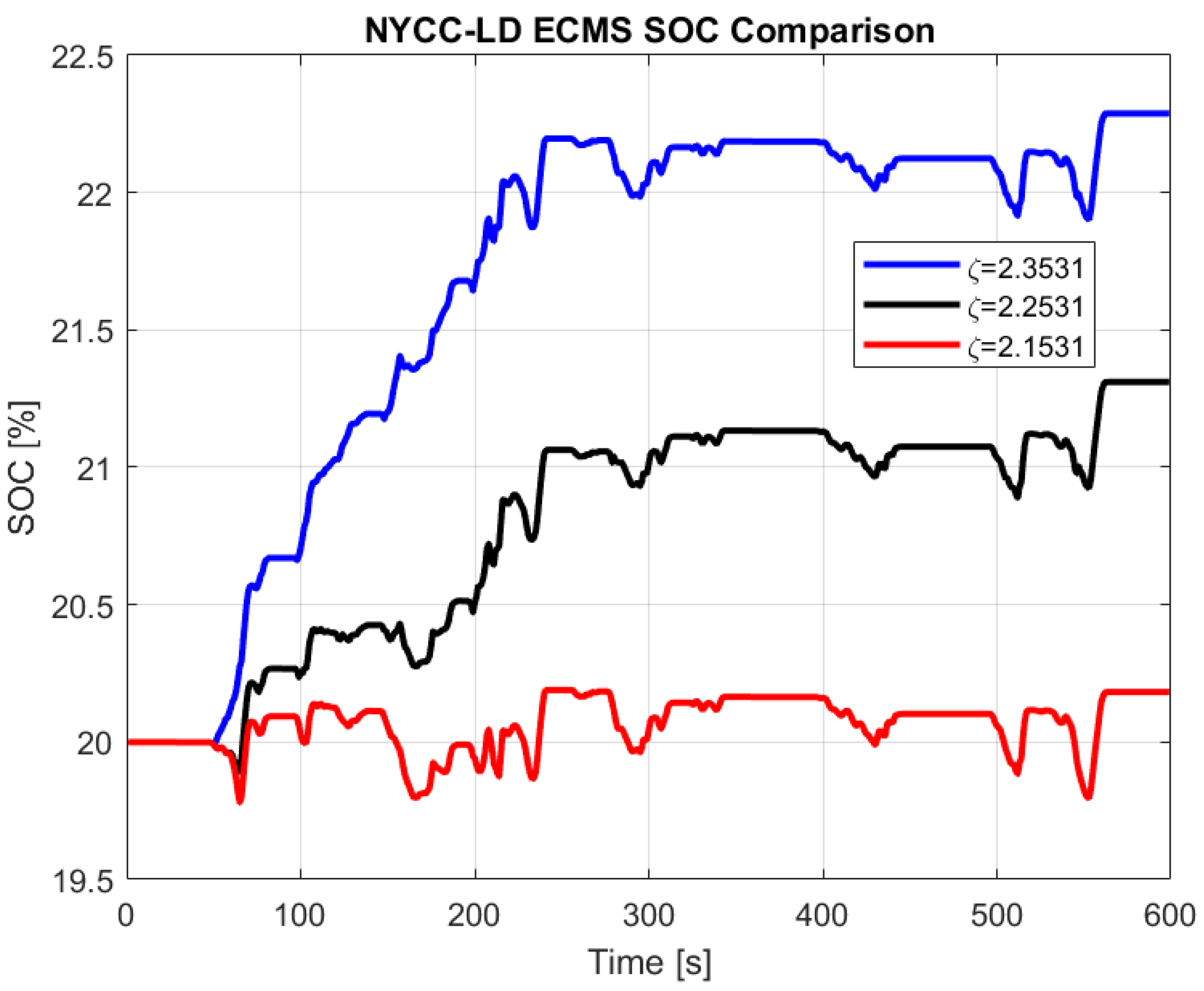
An equivalence factor and penalty function are introduced in the cost function to solve the issue that the $SOC$ constraint cannot be easily applied to the ECMS algorithm directly because $SOC$ is a cumulative result of all the previous steps while ECMS calculates the optimal result based on only the instantaneous information. So we selected the equivalence factor value through trial. To decide the value of the equivalence factor of the ECMS algorithm, different values were tried with the UDDS and NYCC-LD drive cycles. As shown in Figure 1 and Figure 2, the equivalence factor is set as 2.2531, which is the best to sustain final $SOC$ around 20% for both UDDS and NYCC-LD overall. Additionally, this value is utilized for all following simulations. The results show that the ECMS controller is sensitive to equivalence factors by comparing the three $SOC$ curves. Since different $SOC$ behavior will influence the overall $GHG$ emissions, so in real-time application it needs to be calibrated carefully before application.

In Equation (20), the constant equivalence factor is multiplied by the penalty function which can artificially increase or decrease the value around the boundary of the desired $SOC$. In order to allow for asymmetric penalization of the state of energy and maintain the average value at a level closer to one of the boundaries, the penalty value is modified depending on whether the current $SOC$ is above or below the desired $SOC$ as Equation (21) shows [36]. If the present $SOC$ is lower than the target $SOC$, it uses the engine to drive the vehicle and charge the battery, and if the present $SOC$ is higher than the target $SOC$, it uses the e-Motor to drive the vehicle.

$$pen=\left\{\begin{array}{cc}\hfill 1+{\left(\frac{SO{C}_{ref}-SOC\left(t\right)}{SO{C}_{ref}-SO{C}_{min}}\right)}^{2n_{p1}+1},\hfill & \hfill \mathrm{if}SOC\left(t\right)\le SOC{}_{ref}\hfill \\ \hfill 1+{\left(\frac{SOC\left(t\right)-SOC\left(ref\right)}{SO{C}_{max}-SO{C}_{ref}}\right)}^{2n_{p2}+1},\hfill & \hfill \mathrm{if}SOC\left(t\right)\ge SOC{}_{ref}\hfill \end{array}\right.$$

(21)

where $SOC$${}_{ref}$ is the desired nominal value of $SOC$, $SOC$${}_{min}$ and $SOC$${}_{max}$ are the minimum and maximum values of $SOC$, respectively, $n_{p1}$ and $n_{p2}$ are integers.

In this paper, ECMS is implemented by repeating the following steps at each time instant until the end of the drive cycle:

1.

Calculate the torque limits of the e-Motor ($T_{em,min}$, $T_{em,max}$) and the engine ($T_{ice,min}$, $T_{ice,max}$) based on the state of the vehicle at a given instant of time.

2.

Find all possible $T_{em}$ and $T_{ice}$ that satisfy Equation (7).

3.

Calculate all the torque combinations in step 2 based on Equation (20).

4.

Find the optimal $T_{em}$ and $T_{ice}$ combination that minimizes the cost subject to the torque limits.

3.3. Artificial Neural Networks

Artificial neural networks can learn the complicated nonlinear relationships and generate the rule for the controller. In this paper, we applied an ANN to learn the torque split ratio between the ICE and the e-Motor based on the selected inputs and the optimal torque split outputs from the DP algorithm. The ANN model is developed by using the MATLAB DEEP LEARNING toolbox. There are nine observable physical variables in our study which are the required torque by the vehicle ($T_{req}$), engine torque ($T_{ice}$), engine speed (${\omega }_{ice}$), e-Motor torque ($T_{em}$), e-Motor speed (${\omega }_{em}$), vehicle speed (v), vehicle acceleration, battery $SOC$ ($SOC$), and gear number (N${}_g$). Based on these observable variables, we performed the correlation analysis (more detailed information can be found in [31]). In general, if two of the observable variables have a very high correlation, just one of them will be utilized to eliminate multicollinearity. From the correlation analysis, a total of six input variables are selected for the ANN controller [31]. The torque split value is the output that targets the DP optimal results. The schematic is shown in Figure 3.

A total of 31 city cycles with over 30,000 data points are used to train and validate the ANN models which are listed in Appendix A Table A1. The training set is used to train the ANN model and generate the control law for the controller; the validation set is used to check the ANN controller’s performance and determine when to stop training.

The ANN model topology schematic example is shown in Figure 4. This is a two hidden-layer ANN model which consists of an input normalization layer, two hidden layers, an output layer, and an output denormalization layer.

Here, the input normalization layer will map the inputs from the actual value to the per-unit value, while the output denormalization layer does the opposite. To constrain the torque split value in the range from −1 to +1, the tanh activation function is set for all the hidden layers and the output layer. The activation functions can be expressed as:

$$Z_1=\tan \mathrm{h}(W_1\ast x+b_1)$$

(22)

$$Z_2=\tan \mathrm{h}(W_2\ast Z_1+b_2)$$

(23)

$$Y_{predict}=\tan \mathrm{h}(W_3\ast Z_2+b_3)$$

(24)

where x is the normalized input; $Z_1$, $Z_2$, and $Y_{predict}$ are the outputs of the first hidden layer, the second hidden layer, and the output layer, respectively; $W_1$, $W_2$, $W_3$, $b_1$, $b_2$, and $b_2$ are the weight matrices and bias vectors, and the subscript of the number corresponds to each layer.

Different combinations of hidden layers and nodes are utilized, and their results are compared and analyzed. Deciding the best ANN models is challenging and many different measurements can be used to evaluate the training performance of the ANN model [37,38,39]. In this paper, we used the training mean square error (MSE) to evaluate the ANN models. Based on the training MSE of torque split value, the best ones are selected among all the ANN controllers.

First, we trained and compared five ANNs models which use different hidden layers but the same number of hidden nodes in each hidden layer, with detailed information shown in Appendix

Table A2. Multi-layer ANN training results comparison.

ANN	L1	L2	L3	L4	L5	Training MSE	#Parameters
ANN1-8	8	-	-	-	-	3.88 × ${10}^{-3}$	65
ANN2-8-8	8	8	-	-	-	2.94 × ${10}^{-4}$	137
ANN3	8	8	8	-	-	3.34 × ${10}^{-4}$	209
ANN4	8	8	8	8	-	1.53 × ${10}^{-4}$	281
ANN5	8	8	8	8	8	1.17 × ${10}^{-4}$	353

. Figure 5 shows the training results. Since the computer is binary based, the number of hidden nodes is set based on the n^th power of 2. The number following “ANN” represents the number of hidden layers. For example, ANN3 represents the ANN controller with three hidden layers and eight hidden nodes in each hidden layer. ANN1-8 represents a single hidden layer with eight hidden nodes. ANN2-8-8 represents two hidden-layer ANNs, and eight hidden nodes in the first and second hidden layer, respectively.

Figure 5 shows the trend that with the same number of hidden nodes in each hidden layer, the more hidden layers, the smaller the training MSE will be. The potential reason can be that with the same number of hidden nodes, more hidden layers can help it to learn the data relationships. However, more hidden layers will increase the number of parameters which will slow down the computation time for some computation time-critical applications. ANN5 has the minimum training MSE and it will be used to compare with DP and ECMS in the results comparison section. The single hidden-layer ANN1-8 shows the worst training results compared to the others. The potential reason can be that with multiple input variables, a single hidden layer with a small number of hidden nodes may not be able to learn the non-linear relationships well. However, it may be optimized by increasing the number of hidden nodes for the single hidden-layer structure. Therefore, nine single hidden-layer ANN models with different numbers of hidden nodes are developed and investigated. Appendix A 

Table A3. Single-layer ANN training results comparison.

ANN	L1	Training MSE	#Parameters
ANN1-1	1	1.69 × ${10}^{-1}$	9
ANN1-2	2	6.14 × ${10}^{-2}$	17
ANN1-4	4	1.21 × ${10}^{-2}$	33
ANN1-8	8	3.88 × ${10}^{-3}$	65
ANN1-16	16	2.56 × ${10}^{-3}$	129
ANN1-32	32	6.60 × ${10}^{-4}$	257
ANN1-64	64	2.88 × ${10}^{-3}$	513
ANN1-128	128	5.67 × ${10}^{-3}$	1025
ANN1-256	256	4.54 × ${10}^{-3}$	2049

shows the detailed information. The training results are shown in Figure 6. Additionally, the naming rule is similar to the previous, ANN1 represents the single-hidden-layer ANN and the following number represents the number of hidden nodes. For example, ANN1-32 represents a single hidden layer with 32 hidden nodes.

In Figure 6, the results matched our conclusion about the single hidden-layer ANN. It shows that increasing the number of hidden nodes can efficiently improve the training performance. The ANN1-32 with minimum training MSE will be used for the comparison of the results with DP and ECMS. However, ANN1-32 training MSE is 4.64 times that of ANN5. However, if the 10${}^{-4}$ MSE magnitude is acceptable, we can take more benefit from the fewer number of parameters of ANN1-32, which is 27.2% less than ANN5, when it comes to training time. However, ANN1-32 is still worse than ANN2-8-8 overall. Therefore, we further investigated the hyper-parameters effects with two hidden-layer ANNs.

We developed 11 two-hidden-layer ANN models. First, we fixed the number of hidden nodes in the second hidden layer, then changed the number of hidden nodes in the first hidden layer. After that, we used the same method to investigate the effects of the number of hidden nodes in the second hidden layer. The detailed information is listed in Appendix A 

Table A4. Two-hidden-layer ANN training results comparison.

ANN	L1	L2	Training MSE	#Parameters
ANN2-1-8	1	8	6.20 × ${10}^{-2}$	32
ANN2-2-8	2	8	7.86 × ${10}^{-4}$	47
ANN2-4-8	4	8	7.45 × ${10}^{-4}$	77
ANN2-8-8	8	8	2.94 × ${10}^{-4}$	137
ANN2-16-8	16	8	4.22 × ${10}^{-4}$	257
ANN2-32-8	32	8	4.52 × ${10}^{-4}$	497
ANN2-8-1	8	1	5.34 × ${10}^{-3}$	67
ANN2-8-2	8	2	3.22 × ${10}^{-3}$	77
ANN2-8-4	8	4	1.94 × ${10}^{-3}$	97
ANN2-8-16	8	16	1.96 × ${10}^{-4}$	217
ANN2-8-32	8	32	1.77 × ${10}^{-4}$	377

.

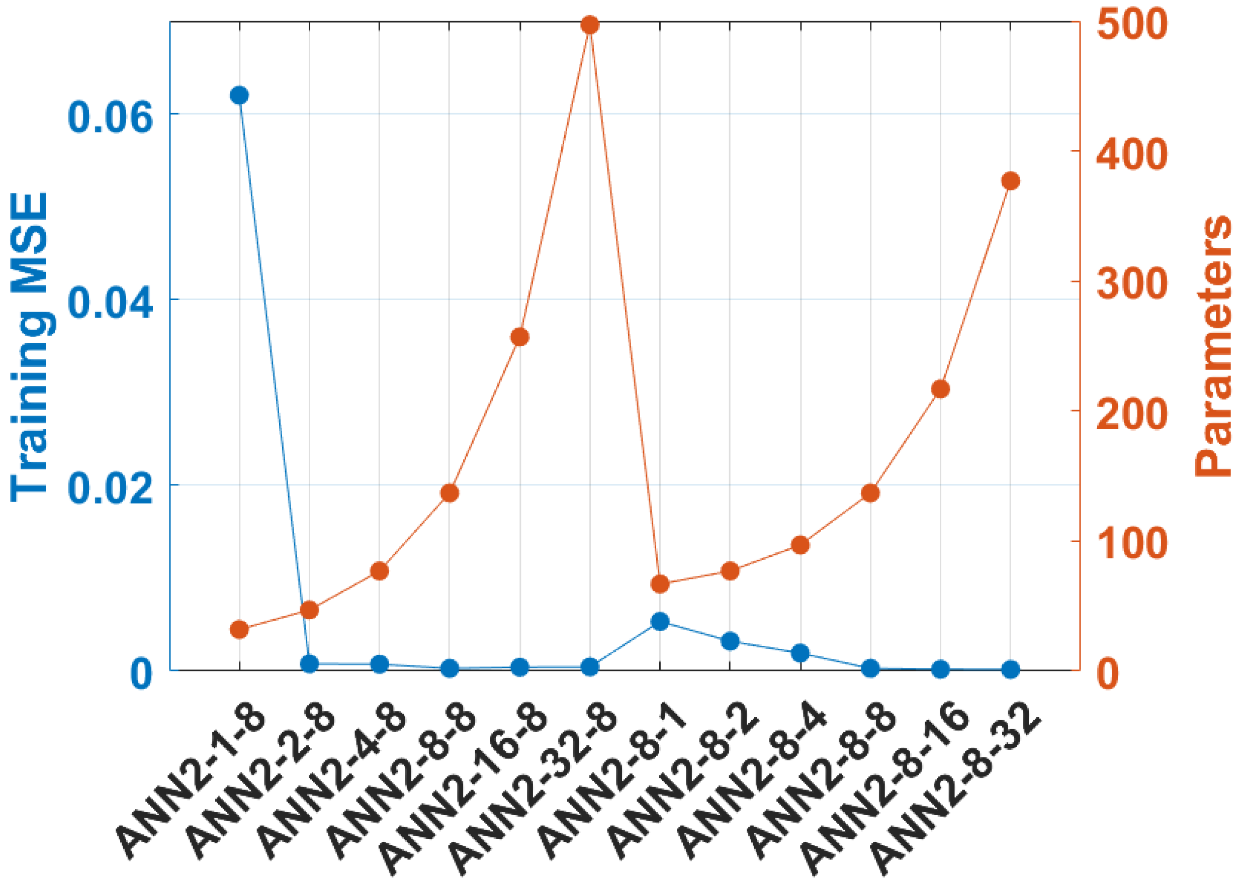
Figure 7 shows the training results of two hidden-layer ANNs. The naming rule is similar to before, ANN2 represents ANN with two hidden layers and the following number indicates the number of hidden nodes in the first hidden layer, and the third number indicates the number of hidden nodes in the second hidden layer. For example, ANN2-8-32 indicates 2 hidden layers, 8 hidden nodes in the first hidden layer, and 32 hidden nodes in the second hidden layer. ANN2-2-32 has the minimum training MSE and is followed by ANN2-8-8. Although ANN2-8-8 training MSE is 66.1% larger than ANN2-2-32 and 1.51 times that ANN5, with the 10${}^{-4}$ training MSE magnitude, ANN2-8-8 has 63.67% fewer parameters than ANN2-2-32 and 61.19% than ANN5. In addition, it shows that for a two-hidden-layer ANN, it is more efficient to change the number of hidden nodes in the second hidden layer than in the first hidden layer. Figure 7 also shows the trend that it is more efficient to modify the number of hidden layers to get better training MSE results than increase the number of nodes in the single hidden-layer structure. This finding is also consistent with the conclusion in [28].

ANN2-8-8, ANN5, ANN1-32, and ANN2-8-32 controllers will be used for comparison with DP and ECMS in the following section.

4. Results Comparison

The UDDS and NYCC-LD urban drive cycles, which are not included in the training set, are used for validation by comparing the results with DP and ECMS. The UDDS drive cycle simulates an urban route of 12.07 km (7.5 miles) with frequent stops, and the maximum speed is 91.25 km/h (56.7 mph). Additionally, the average speed of UDDS is 31.5 km/h (19.6 mph). The NYCC-LD also simulates low-speed urban driving with frequent stops, but with a shorter total distance of 1.89 km (1.18 miles), a lower maximum speed of 44.6 km/h (27.7 mph), and a lower average speed of 11.4 km/h (7.1 mph) compared to UDDS drive cycle. The drive cycles’ speed profiles are shown in Figure 8.

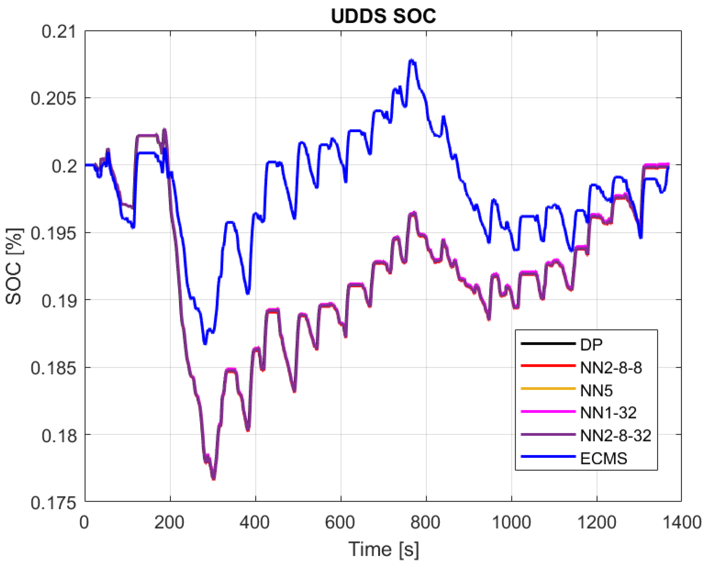
There are five metrics for the comparison: fuel consumption (liter), fuel $GHG$ emissions (gram), electricity $GHG$ emissions (gram), total $GHG$ emissions which is the sum of fuel and electricity $GHG$ emissions, and the terminal $SOC$ status. DP is the baseline for the result comparison. In general, the closer the controller’s result is to DP’s, the better the controller is. Figure 9 shows $SOC$ results of the UDDS drive cycle for each control strategy. Fuel consumption, fuel $GHG$ emissions, electricity $GHG$ emissions, and total $GHG$ emissions are summarized in

Table 4. UDDS results comparison.

Control Strategy	Fuel Consumption (Liter)	Fuel GHG Emissions (g)	Electricity GHG Emissions (g)	Total GHG Emissions (g)	$\mathit{S}\mathit{O}\mathit{C}$${}_{\mathit{tf}}$
DP	0.5100	1.81 × ${10}^3$	0	1.81 × ${10}^3$	0.2000
ECMS	0.5444	1.93 × ${10}^3$	1.569	1.93 × ${10}^3$	0.1998
ANN2-8-8	0.5103	1.81 × ${10}^3$	1.282	1.81 × ${10}^3$	0.1998
ANN5	0.5101	1.81 × ${10}^3$	0.140	1.81 × ${10}^3$	0.2000
ANN1-32	0.5106	1.81 × ${10}^3$	−0.678	1.81 × ${10}^3$	0.2001
ANN2-8-32	0.5097	1.81 × ${10}^3$	0.902	1.81 × ${10}^3$	0.1999

.

Since we set the DP’s terminal $SOC$ to the same 20% as the initial $SOC$, ANNs replicate DP’s under urban driving conditions. Therefore, the electricity $GHG$ emissions of ANNs should be virtually zero. The very small negative or positive $GHG$ emissions value will only occur when the terminal $SOC$ is slightly higher or lower than the preset 20% $SOC$. If the terminal $SOC$ is slightly lower than 20%, which means the battery slightly discharges and the electrical energy is consumed, it will cause a very small positive electrical $GHG$ emission. While in the case of terminal $SOC$ slightly higher than 20%, which means the battery is slightly charged, it will have a very small negative electrical $GHG$ emissions value since it stores the electricity energy instead of consuming it.

From Figure 9, all the ANN controllers show a similar $SOC$ behavior to DP. ECMS has a slightly higher average $SOC$ value compared to DP and ANNs. ANN controllers generate 6.22% less total $GHG$ emissions than that of ECMS, as shown in Table 4. In addition, all the controllers’ $SOC$s are within 0.1% deviation compared to DP.

Figure 10 shows the $SOC$ comparison results of NYCC-LD. Fuel consumption, fuel $GHG$ emissions, electricity $GHG$ emissions, and total $GHG$ emissions are listed in

Table 5. NYCC-LD results comparison.

Control Strategy	Fuel Consumption (Liter)	Fuel GHG Emissions (g)	Electricity GHG Emissions (g)	Total GHG Emissions (g)	$\mathit{SOC}$${}_{\mathit{tf}}$
DP	0.1139	404	−0.045	404	0.2000
ECMS	0.1609	572	−108.180	463	0.2131
ANN2-8-8	0.1146	407	0.020	407	0.2000
ANN5	0.1140	405	−0.960	404	0.2001
ANN1-32	0.1139	405	−0.453	404	0.2001
ANN2-8-32	0.1139	405	−0.264	404	0.2000

.

From Figure 10, ANN controllers show similar results to UDDS and all the ANN controllers show similar $SOC$ behavior compared to DP. However, ECMS shows a different $SOC$ behavior compared to DP and ANNs, with a 6.6% deviation. Moreover, ANN controllers have 12.1% less total $GHG$ emissions than ECMS at least under this drive cycle, as shown in Table 5.

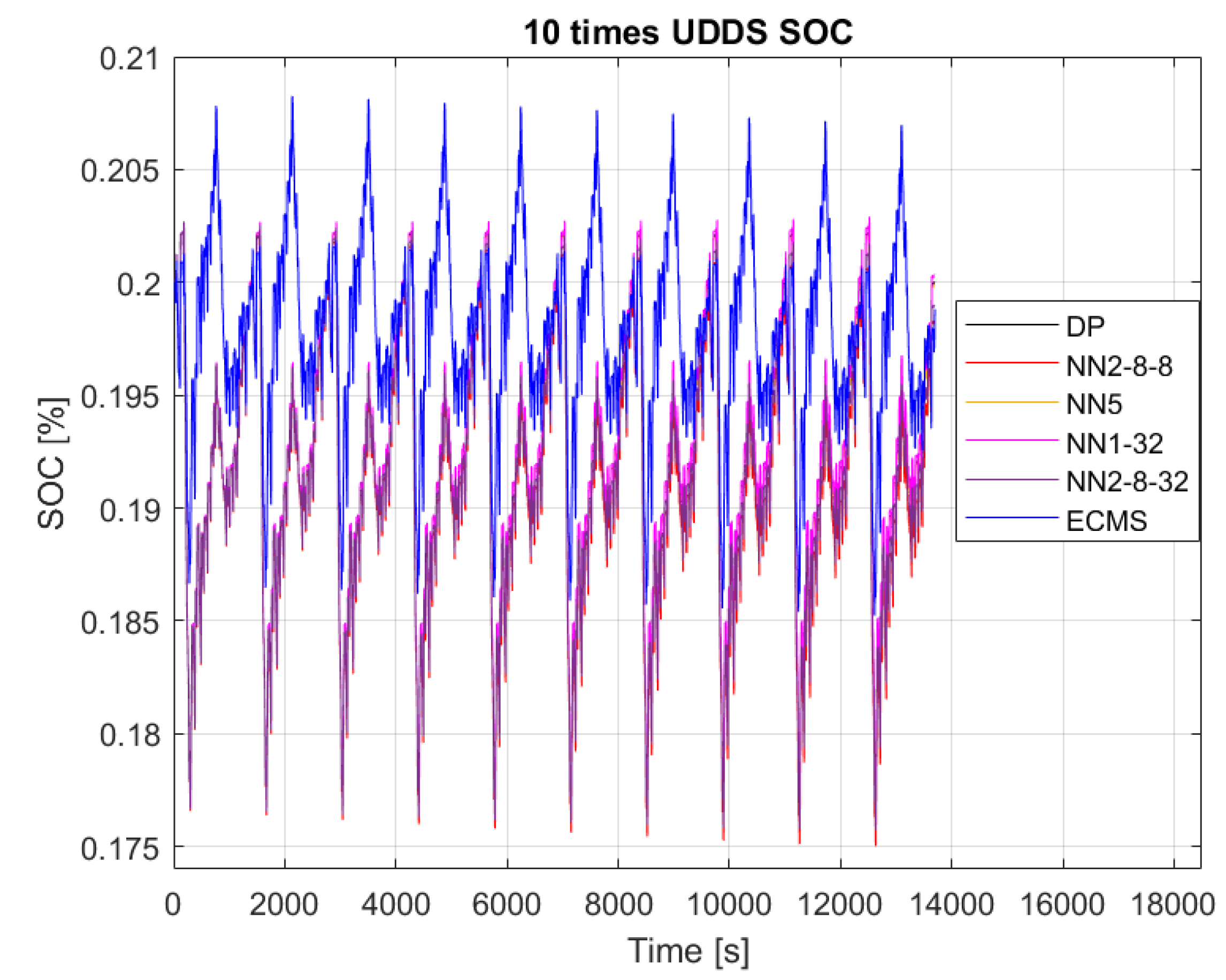
In order to check the robustness of each control strategy, UDDS and NYCC-LD drive cycles are repeated 10 times. Figure 11 and Figure 12 are the $SOC$ results of UDDS and NYCC-LD, respectively. Additionally, the results are listed in

Table 6. Results comparison for UDDS repeated 10 times.

Control Strategy	Fuel Consumption (Liter)	Fuel GHG Emissions (g)	Electricity GHG Emissions (g)	Total GHG Emissions (g)	$\mathit{SOC}$${}_{\mathit{tf}}$
DP	5.0306	1.79 × ${10}^4$	0	1.79 × ${10}^4$	0.2000
ECMS	5.4503	1.94 × ${10}^4$	9.910	1.94 × ${10}^4$	0.1988
ANN2-8-8	5.0328	1.79 × ${10}^4$	13.919	1.79 × ${10}^4$	0.1983
ANN5	5.0320	1.79 × ${10}^4$	0.854	1.79 × ${10}^4$	0.1999
ANN1-32	5.0359	1.79 × ${10}^4$	−2.904	1.79 × ${10}^4$	0.2004
ANN2-8-32	5.0275	1.79 × ${10}^4$	8.320	1.79 × ${10}^4$	0.1990

and

Table 7. Results comparison for NYCC-LD repeated 10 times.

Control Strategy	Fuel Consumption (Liter)	Fuel GHG Emissions (g)	Electricity GHG Emissions (g)	Total GHG Emissions (g)	$\mathit{SOC}$${}_{\mathit{tf}}$
DP	1.1367	4.04 × ${10}^3$	0	4.04 × ${10}^3$	0.2000
ECMS	1.2065	4.28 × ${10}^3$	−246	4.04 × ${10}^3$	0.2298
ANN2-8-8	1.1447	4.06 × ${10}^3$	−67.266	4.00 × ${10}^3$	0.2081
ANN5	1.1379	4.04 × ${10}^3$	−20.479	4.02 × ${10}^3$	0.2025
ANN1-32	1.1373	4.04 × ${10}^3$	−64.891	3.97 × ${10}^3$	0.2079
ANN2-8-32	1.1372	4.04 × ${10}^3$	−0.859	4.04 × ${10}^3$	0.2001

, respectively. In Figure 12, ECMS shows a different $SOC$ to DP and ANNs, and its total $GHG$ emission is 10.06% higher than the other controllers under the UDDS 10 times drive cycle. This shows similar trends in UDDS and NYCC-LD which illustrates the significance of the equivalence factor value selection. In Table 7, ANN2-8-8, ANN5, and ANN1-32 have lower total $GHG$ emissions because of the higher final $SOC$ at the end of the drive cycle which means they stored more electrical energy for future use. Overall, the ANN controllers still show similar $SOC$ behavior and total $GHG$ emissions to DP which is consistent with the UDDS and NYCC-LD performance. Furthermore, all ANN controllers have the same sum of total $GHG$ emissions in all four driving cycles in this section compared to DP. However, ANN5 has the best performance among the ANN controllers if we take $SOC$ constraints into consideration. ANN2-8-32 comes next, then ANN2-8-8. This also indicates that multiple hidden layers may help to improve the ANN’s performance.

5. Conclusions and Future Works

In this paper, we further investigated and extended our previous study, and we focused on urban driving conditions with a low initial $SOC$ condition of 20%. We applied the DP controller and set it as the baseline for the comparison. ANNs are developed and analyzed, and then compared against the DP solution as well as ECMS. The effects of ANN hyper-parameters were investigated. We concluded that:

• ECMS showed sensitivity to equivalence factor values as shown in UDDS and NYCC-LD drive cycles.
• Compared with the multi-hidden-layer ANN structure, the MSE training results of the single-hidden-layer ANN controller are poor. During artificial neural network training, changing the number of hidden layers may be a more efficient way.
• The single-hidden-layer ANN’s training MSE performance can be optimized by increasing the number of hidden nodes. However, the training MSE may not be more competitive than multiple hidden-layer structures.
• All the selected ANNs are within 0.2% $GHG$ emissions and 1.1% $SOC$ error compared to DP which indicates that ANNs are almost as good as the DP solutions, and it is implementable in real-time.

Our future works will be:

• Set up the controllers for implementation on the MicroAutoBox in the vehicle.
• Run them on our real test vehicle with city drive cycle conditions.
• Evaluate the results and optimize the controllers based on the tests.

References

- U.S. Environmental Protection Agency. Overview of Greenhouse Gases. Available online: https://www.epa.gov/ghgemissions/overview-greenhouse-gases (accessed on 25 May 2022).
- Malikopoulos, A.A. Supervisory power management control algorithms for hybrid electric vehicles: A survey. IEEE Trans. Intell. Transp. Syst. 2014, 15, 1869–1885. [Google Scholar] [CrossRef]
- Mi, C.; Masrur, M.A. Hybrid Electric Vehicles: Principles and Applications with Practical Perspectives; John Wiley & Sons: Hoboken, NJ, USA, 2017. [Google Scholar]
- Palmer, K.; Tate, J.E.; Wadud, Z.; Nellthorp, J. Total cost of ownership and market share for hybrid and electric vehicles in the UK, US and Japan. Appl. Energy 2018, 209, 108–119. [Google Scholar] [CrossRef]
- Balali, Y.; Stegen, S. Review of energy storage systems for vehicles based on technology, environmental impacts, and costs. Renew. Sustain. Energy Rev. 2021, 135, 110185. [Google Scholar] [CrossRef]
- Bayindir, K.Ç.; Gözüküçük, M.A.; Teke, A. A comprehensive overview of hybrid electric vehicle: Powertrain configurations, powertrain control techniques and electronic control units. Energy Convers. Manag. 2011, 52, 1305–1313. [Google Scholar] [CrossRef]
- Ehsani, M.; Gao, Y.; Longo, S.; Ebrahimi, K.M. Modern Electric, Hybrid Electric, and Fuel Cell Vehicles; CRC Press: Boca Raton, FL, USA, 2018. [Google Scholar]
- Sharer, P.B.; Rousseau, A.; Karbowski, D.; Pagerit, S. Plug-in Hybrid Electric Vehicle Control Strategy: Comparison Between EV and Charge-Depleting Options; SAE International: Warrendale, PA, USA, 2008; Volume 32. [Google Scholar]
- Mohamed, N.; Aymen, F.; Ali, Z.M.; Zobaa, A.F.; Abdel Aleem, S.H. Efficient power management strategy of electric vehicles based hybrid renewable energy. Sustainability 2021, 13, 7351. [Google Scholar] [CrossRef]
- Guan, J.C.; Chen, B.C.; Wu, Y.Y. Design of an adaptive power management strategy for range extended electric vehicles. Energies 2019, 12, 1610. [Google Scholar] [CrossRef] [Green Version]
- Xue, Q.; Zhang, X.; Teng, T.; Zhang, J.; Feng, Z.; Lv, Q. A comprehensive review on classification, energy management strategy, and control algorithm for hybrid electric vehicles. Energies 2020, 13, 5355. [Google Scholar] [CrossRef]
- Xu, N.; Kong, Y.; Chu, L.; Ju, H.; Yang, Z.; Xu, Z.; Xu, Z. Towards a smarter energy management system for hybrid vehicles: A comprehensive review of control strategies. Appl. Sci. 2019, 9, 2026. [Google Scholar] [CrossRef] [Green Version]
- Zhang, F.; Wang, L.; Coskun, S.; Pang, H.; Cui, Y.; Xi, J. Energy management strategies for hybrid electric vehicles: Review, classification, comparison, and outlook. Energies 2020, 13, 3352. [Google Scholar] [CrossRef]
- Jeong, J.; Kim, N.; Lim, W.; Park, Y.I.; Cha, S.W.; Jang, M.E. Optimization of power management among an engine, battery and ultra-capacitor for a series HEV: A dynamic programming application. Int. J. Automot. Technol. 2017, 18, 891–900. [Google Scholar] [CrossRef]
- Yang, Y.; Pei, H.; Hu, X.; Liu, Y.; Hou, C.; Cao, D. Fuel economy optimization of power split hybrid vehicles: A rapid dynamic programming approach. Energy 2019, 166, 929–938. [Google Scholar] [CrossRef]
- Lee, H.; Song, C.; Kim, N.; Cha, S.W. Comparative analysis of energy management strategies for HEV: Dynamic programming and reinforcement learning. IEEE Access 2020, 8, 67112–67123. [Google Scholar] [CrossRef]
- Oliva, D.; Abd Elaziz, M.; Elsheikh, A.H.; Ewees, A.A. A review on meta-heuristics methods for estimating parameters of solar cells. J. Power Sources 2019, 435, 126683. [Google Scholar] [CrossRef]
- Abd Elaziz, M.; Elsheikh, A.H.; Oliva, D.; Abualigah, L.; Lu, S.; Ewees, A.A. Advanced metaheuristic techniques for mechanical design problems. Arch. Comput. Methods Eng. 2022, 29, 695–716. [Google Scholar] [CrossRef]
- Huang, Y.; Wang, H.; Khajepour, A.; He, H.; Ji, J. Model predictive control power management strategies for HEVs: A review. J. Power Sources 2017, 341, 91–106. [Google Scholar] [CrossRef]
- Wang, Y.; Advani, S.G.; Prasad, A.K. A comparison of rule-based and model predictive controller-based power management strategies for fuel cell/battery hybrid vehicles considering degradation. Int. J. Hydrogen Energy 2020, 45, 33948–33956. [Google Scholar] [CrossRef]
- Paganelli, G.; Guerra, T.M.; Delprat, S.; Santin, J.J.; Delhom, M.; Combes, E. Simulation and assessment of power control strategies for a parallel hybrid car. Proc. Inst. Mech. Eng. Part J. Automob. Eng. 2000, 214, 705–717. [Google Scholar] [CrossRef]
- Paganelli, G.; Tateno, M.; Brahma, A.; Rizzoni, G.; Guezennec, Y. Control development for a hybrid-electric sport-utility vehicle: Strategy, implementation and field test results. In Proceedings of the 2001 American Control Conference (Cat. No. 01CH37148), Arlington, VA, USA, 25–27 June 2001; Volume 6, pp. 5064–5069. [Google Scholar]
- Paganelli, G.; Delprat, S.; Guerra, T.M.; Rimaux, J.; Santin, J.J. Equivalent consumption minimization strategy for parallel hybrid powertrains. In Proceedings of the EEE 55th Vehicular Technology Conference, VTC Spring 2002 (cat. No. 02CH37367), Arlington, VA, USA, 25–27 June 2002; Volume 4, pp. 2076–2081. [Google Scholar]
- Zeng, Y.; Cai, Y.; Kou, G.; Gao, W.; Qin, D. Energy management for plug-in hybrid electric vehicle based on adaptive simplified-ECMS. Sustainability 2018, 10, 2060. [Google Scholar] [CrossRef] [Green Version]
- Rezaei, A.; Burl, J.B.; Zhou, B. Estimation of the ECMS equivalent factor bounds for hybrid electric vehicles. IEEE Trans. Control Syst. Technol. 2017, 26, 2198–2205. [Google Scholar] [CrossRef]
- Guan, J.C.; Chen, B.C. Adaptive power management strategy based on equivalent fuel consumption minimization strategy for a mild hybrid electric vehicle. In Proceedings of the Vehicle Power and Propulsion Conference (VPPC), Hanoi, Vietnam, 14–17 October 2019; pp. 1–4. [Google Scholar]
- Pulpeiro González, J.; Ankobea-Ansah, K.; Peng, Q.; Hall, C.M. On the integration of physics-based and data-driven models for the prediction of gas exchange processes on a modern diesel engine. Proc. Inst. Mech. Eng. Part J. Automob. Eng. 2022, 236, 857–871. [Google Scholar] [CrossRef]
- Peng, Q.; Huo, D.; Hall, C.M. Neural network-based air handling control for modern diesel engines. Proc. Inst. Mech. Eng. Part D J. Automob. Eng. 2022, 09544070221083367. [Google Scholar] [CrossRef]
- Chen, Z.; Mi, C.C.; Xu, J.; Gong, X.; You, C. Energy management for a power-split plug-in hybrid electric vehicle based on dynamic programming and neural networks. IEEE Trans. Veh. Technol. 2013, 63, 1567–1580. [Google Scholar] [CrossRef]
- Munoz, P.M.; Correa, G.; Gaudiano, M.E.; Fernández, D. Energy management control design for fuel cell hybrid electric vehicles using neural networks. Int. J. Hydrogen Energy 2017, 42, 28932–28944. [Google Scholar] [CrossRef]
- Gupta, R.; Meckl, P.H. Model development for a parallel through-the-road plug-in hybrid electric vehicle. In Proceedings of the American Control Conference (ACC), Boston, MA, USA, 6–8 July 2016; pp. 4551–4556. [Google Scholar]
- Argonne National Laboratory. GREET WTW Calculator. Available online: https://greet.es.anl.gov/index.php?content=sampleresults (accessed on 25 May 2022).
- Pachernegg, S. A Closer Look at The Willans-Line; Technical Report, SAE Technical Paper; SAE: Warrendale, PA, USA, 1969. [Google Scholar]
- Newman, K.; Kargul, J.; Barba, D. Benchmarking and Modeling of a Conventional Mid-Size Car Using ALPHA; SAE Technical Paper; SAE: Warrendale, PA, USA, 2015; pp. 1–1140. [Google Scholar]
- Sundstrom, O.; Guzzella, L. A generic dynamic programming Matlab function. In Proceedings of the Control Applications,(CCA) & Intelligent Control, (ISIC), St. Petersburg, Russia, 8–10 July 2009; pp. 1625–1630. [Google Scholar]
- Serrao, L.; Onori, S.; Rizzoni, G. A comparative analysis of energy management strategies for hybrid electric vehicles. J. Dyn. Syst. Meas. Control 2011, 133, 031012. [Google Scholar] [CrossRef] [Green Version]
- Elsheikh, A.H.; Sharshir, S.W.; Abd Elaziz, M.; Kabeel, A.; Guilan, W.; Haiou, Z. Modeling of solar energy systems using artificial neural network: A comprehensive review. Sol. Energy 2019, 180, 622–639. [Google Scholar] [CrossRef]
- Elsheikh, A.H.; Abd Elaziz, M.; Das, S.R.; Muthuramalingam, T.; Lu, S. A new optimized predictive model based on political optimizer for eco-friendly MQL-turning of AISI 4340 alloy with nano-lubricants. J. Manuf. Process. 2021, 67, 562–578. [Google Scholar] [CrossRef]
- Elsheikh, A.H.; Abd Elaziz, M.; Vendan, A. Modeling ultrasonic welding of polymers using an optimized artificial intelligence model using a gradient-based optimizer. Weld. World 2022, 66, 27–44. [Google Scholar] [CrossRef]
Figure 1.
ECMS equivalence factor comparison for UDDS.
Figure 2.
ECMS equivalence factor comparison for NYCC-LD.
Figure 3.
ANN supervisory controller.
Figure 4.
ANN model topology illustration.
Figure 5.
Training results of multi-hidden-layer ANN with 8 hidden nodes.
Figure 6.
Training results for single-hidden-layer ANN.
Figure 7.
Training results for two-hidden-layer ANNs.
Figure 8.
Speed profiles of UDDS and NYCC-LD.
Figure 9.
results for UDDS drive cycle.
Figure 10.
results for NYCC-LD drive cycle.
Figure 11.
results for UDDS repeated 10 times.
Figure 12.
results for NYCC-LD repeated 10 times.