A Novel Virtual Sensor Modeling Method Based on Deep Learning and Its Application in Heating, Ventilation, and Air-Conditioning System

Abstract

Realizing the dynamic redundancy of sensors is of great significance to ensure the energy saving and normal operation of the heating, ventilation, and air-conditioning (HVAC) system. Building a virtual sensor model is an effective method of redundancy and fault tolerance for hardware sensors. In this paper, a virtual sensor modeling method combining the maximum information coefficient (MIC) and the spatial–temporal attention long short-term memory (STA-LSTM) is proposed, which is named MIC-STALSTM, to achieve the dynamic and nonlinear modeling of the supply and return water temperature at both ends of the chiller. First, MIC can extract the influencing factors highly related to the target variables. Then, the extracted impact factors via MIC are used as the input variables of the STA-LSTM algorithm in order to construct an accurate virtual sensor model. The STA-LSTM algorithm not only makes full use of the LSTM algorithm’s advantages in handling historical data series information, but also achieves adaptive estimation of different input variable feature weights and different hidden layer temporal correlations through the attention mechanism. Finally, the effectiveness and feasibility of the proposed method are verified by establishing two virtual sensors for different temperature variables in the HVAC system.

1. Introduction

Heating, ventilation, and air-conditioning (HVAC) systems, which ensure a good indoor environment and air quality, are frequently used in commercial, residential, and industrial buildings. HVAC systems can be thought of as a complex network of several interrelated subsystems, each of which includes several mechanical components and a large number of sensors. Common sensors used in HVAC systems include humidity sensors, CO${}_2$ sensors, temperature sensors, and particulate matter (PM) sensors, etc. [1]. These sensors are constantly monitoring the real-time operation of the system and feeding the monitored information back to the control system. Correct sensor values are the basis for the control system to be capable of making appropriate decisions. However, sensors used in HVAC systems are inevitably prone to different types of faults (e.g., bias, drift, and abrupt failures). Errors generated by faulty sensors have considerable effects on the control behavior of HVAC systems, and lead to increased energy consumption and reduced thermal comfort [2]. Therefore, it is essential to construct virtual sensors as effective alternatives to faulty sensors in HVAC systems.

Generally, the modeling methods of virtual sensors are divided into two categories, including model-based methods and data-driven methods. Model-based methods require mathematical equations to define the relationship between input and output variables. However, due to the complexity of modern HVAC systems, it is difficult to use mathematical equations to establish an accurate virtual sensor model. In contrast, data-driven methods do not need to establish an accurate mathematical model, and only need to obtain a decision function through the processing of historical observation data. The accuracy of the final results is ensured by adjusting the decision function continuously. Plenty of multivariate statistical methods and machine learning methods based on data-driven are widely used in the development of virtual sensors, such as principal component regression (PCR) [3], partial least squares regression (PLSR) [4], support vector regression (SVR) [5], and multilayer perceptron (MLP) [6]. However, multivariate statistical methods for virtual sensor modeling have significant limitations in dealing with non-linear data. Moreover, MLP frequently suffers from gradient explosion, which may lead to poor modeling performance when the network structure becomes too large and complex. In response to the many problems in multivariate statistical methods and machine learning methods, deep learning has been gradually developed over the past decade and has been very successful in a variety of areas [7,8,9,10], including the modeling of virtual sensors. For example, the gated stacked target-related autoencoder (GSTAE) for virtual sensor modeling was proposed and applied to an industrial case to measure the butane concentration at the bottom of a de-butane tower [11]. An adaptive deep belief network (OAFDBN) was used to build a virtual sensor for the sake of estimating the cetane content in diesel [12].

Among the vast range of deep learning algorithms, the long short-term memory (LSTM), with its unique storage unit and gate structure, can effectively avoid the gradient vanishing in neural networks and better capture the non-linear and dynamic correlations of data in industrial processes. There is no doubt that the superiority shown by LSTM has attracted countless researchers working in the field of virtual sensors. For example, a virtual sensor based on LSTM has been put forward and used in sulfur recovery units (SRU) [13]. As sensors in SRU are highly susceptible to corrosion, the virtual sensor built is an effective alternative to the hardware sensor for estimating the concentration of SO${}_2$ and H${}_2$S in the output gas stream. At the same time, improved algorithms based on LSTM are constantly being proposed. A supervised long short-term memory (SLSTM) capable of dynamically learning hidden states using target and input variables was proposed and the effectiveness of the virtual sensor model built by SLSTM was demonstrated on the penicillin fermentation process [14]. A variable attention-based long short-term memory (VA-LSTM) was proposed for virtual sensor modeling, which focuses on capturing correlations between input variables and the target variable [15]. In the proposed model, different weights are assigned to each input variable depending on the magnitude of the correlation. Ultimately, satisfactory performance for the final distillation point prediction of the heavy naphtha in the hydrocracking process has been achieved.

However, to the best of our knowledge, few studies have been carried out on virtual sensor modeling for HVAC systems. This is because there are still some problems that need to be overcome. For instance, a large amount of sensor data are stored during the operation of HVAC systems, but not all of them contribute to the modeling of virtual sensors. Furthermore, HVAC systems are always in switching operating states. This switching between operating conditions will lead to sudden changes in some sensor data, which have a great impact on the subsequent predictions of virtual sensors. Therefore, this paper proposes an MIC-STALSTM method for handling the two problems described above and frequently encountered in the operation of HVAC systems. The method combines the maximal information coefficient (MIC) and the spatio-temporal attention long short-term memory (STA-LSTM). According to the data collected by the HVAC system, the method uses the MIC to explore the correlation between the remaining variables and the target variables, which are the supply and return water temperature variable at both ends of the chiller. Moreover, the highly correlated impact factors filtered by the MIC are used as the input variables of the subsequent STA-LSTM algorithm to construct a virtual sensor. Finally, the MIC-STALSTM algorithm is validated on a real HVAC system and compared with the LSTM, TA-LSTM, and STA-LSTM for analysis.

The remainder of this paper is organized as follows. In Section 2, the relevant fundamentals of the maximal information coefficient (MIC) and the spatio-temporal attention long short-term memory (STA-LSTM) are briefly summarized. In Section 3, the MIC-STALSTM model combining MIC and STA-LSTM is proposed, and a virtual sensor modeling framework based on MIC-STALSTM is presented. In Section 4, the effectiveness and feasibility of the proposed method are verified in a case study of an HVAC system by constructing virtual sensors for two target temperature variables. Finally, conclusions are drawn in the last section, Section 5.

2. Methodology

In this section, the deep learning framework and some basic algorithms that make up the MIC-STALSTM method are presented in detail.

2.1. Maximal Information Coefficient

When exploring relationships in datasets, traditional correlation coefficient-based methods can only effectively estimate the linear relationships between variables. In contrast, non-linear relationships are more common in actual industrial datasets. MIC is a powerful method to measure the correlation between two variables, which can not only discover linear correlations in datasets, but also explore potential non-linear and non-functional correlations between variables [16,17]. For two variables X and Y, their correlation is calculated via MIC. The first step is to draw a scatter plot of the dataset $D=\{(x_1,y_1),(x_2,y_2),\cdots ,(x_n,y_n)\}$ (where n is the number of samples) on a two-dimensional space. Along the x-axis and y-axis directions, i grids and j grids are, respectively, divided, and the two-dimensional space is divided into $i\times j$ small grids. The scatter plot formed by the dataset D has a corresponding probability distribution $D|G$ on each small grid G [18]. Since there is more than one way to divide the dataset by grid, all existing grid possibilities can be explored through different partitioning schemes. An optimal discretization method can be found and the maximum mutual information (MI) corresponding to the optimal discretization method can be obtained.

$$M{I}^{\ast }(D,i,j)=maxMI\left(D\right|G)$$

(1)

where $MI\left(D\right|G)$ represents the mutual information when the probability distribution is $D|G$. The maximum mutual information value is normalized to the interval $[0,1]$, which can be expressed as:

$$M{\left(D\right)}_{i\times j}=\frac{M{I}^{\ast }(D,i,j)}{lo{g}_{2}min(i,j)}$$

(2)

Then, we select the largest mutual information value after normalization as the MIC value. The calculation of MIC can be expressed as:

$$MIC{\left(D\right)}_{i\times j}=ma{x}_{i\times j<B\left(n\right)}M{\left(D\right)}_{i\times j}$$

(3)

where the resolution of the grid is restricted to $i\times j<B\left(n\right)$ and $B\left(n\right)=n^{0.6}$.

The variables X and Y are independent of each other when the value of MIC equals 0; when the MIC is equal to 1, there is a functional relationship that can be described between the variables X and Y. A prominent feature of MIC is that when MIC is used to detect the correlation between variables, the value measured by MIC will be more concentrated at either ends of the range [0, 1]. Such characteristics allow MIC to better explore the potential relationships between variables than traditional feature selection methods such as the Pearson or Spearman correlation coefficient.

2.2. Spatio-Temporal Attention Long Short-Term Memory

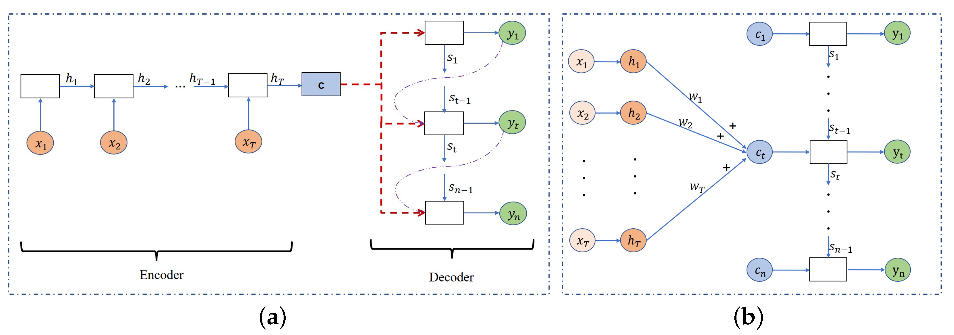
The encoder–decoder (Seq2Seq) is a deep learning framework that is widely used to process time series, which provides a powerful solution for the problem processing of dynamic sequences, and its basic structure is shown in Figure 1a. The encoder–decoder structure firstly needs to compress all the information of the input data sequence into an intermediate vector c with a fixed length through an encoder unit, and then decode the intermediate vector c through a decoder unit to obtain the desired output sequence: $\{y_1,y_2,\cdots ,y_n\}$. The encoder unit and decoder unit in the framework can use any basic neural network framework, such as RNN, GRU, LSTM, and so on.

The encoder–decoder framework has distinct advantages in some areas, such as machine translation, in that this framework can handle the problem of unequal lengths of input and output sequences. However, as the length of the processing sequence increases, the intermediate vector c may lose some key valid information, resulting in a decrease in the accuracy of subsequent decoding. Therefore, for the purpose of addressing the challenge of information loss in the encoder–decoder framework, the attention mechanism was introduced to the basic encoder–decoder framework structure [19]. In this attention-based structure, shown in Figure 1b, the original fixed-length vector c is replaced by a changing vector $c_t$ determined by the current desired output $y_t$.

$$c_t=\sum _{i=1}^T{w}_i·h_i$$

(4)

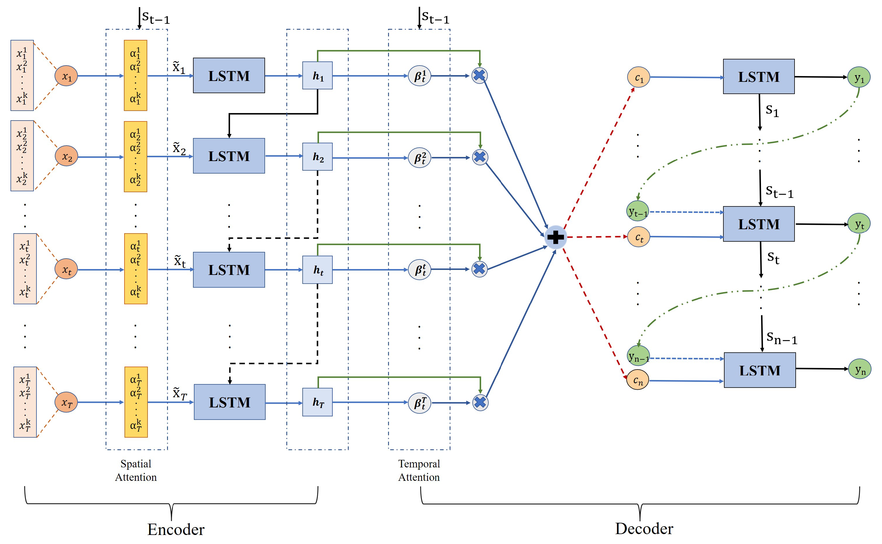
This paper adopts the spatio-temporal attention long short-term memory (STA-LSTM) model; its structure is shown in Figure 2, which introduces the spatial attention mechanism and the temporal attention mechanism on the basic encoder–decoder framework. Firstly, STA-LSTM introduces a spatial attention mechanism on the encoder side, which can assign different spatial attention weights to input variables at different time steps. Its calculation process is as follows.

In time step t, there are samples of k variables: $x_t=[x_t^1,x_t^2,\cdots ,x_t^k]$, where $x_t^k\in R^3$, the spatial weight corresponding to k variables ${\gamma }_t=[{\gamma }_t^1,{\gamma }_t^2,\cdots ,{\gamma }_t^k$], where the formula for calculating the spatial weight corresponding to the ith variable is as follows:

$${\gamma }_t^i=U_s^{1}tanh(W^{x1}{x}_t^i+W^{h1}{s}_{t-1}+b_1)$$

(5)

where $i\in [1,k]$, $U_s^1$, $W^{x1}$, $W^{h1}$ are the parameters that the network needs to learn through training, $b_1$ is the bias, $s_{t-1}$ is the hidden variable from the LSTM hidden layer, and $tanh$ is the double curve activation function. We normalize the spatial attention weight of the ith variable by Equation (6) in order to ensure that the sum of the spatial attention weight of all input variables is 1 at time step t.

$${\alpha }_t^i=\frac{exp\left({\gamma }_t^i\right)}{{\sum }_{i=1}^{k}exp\left({\gamma }_t^j\right)}$$

(6)

The spatial weights assigned to different inputs finally determine the amount of information flowing to the encoder part of the LSTM network. The larger the spatial weight, the more important the corresponding input features are for predicting the output. Then, we assign their corresponding weights to the input variables, $[x_t^1,x_t^2,\cdots ,x_t^k]$, and obtain a new input sequence by weighting, as shown in Equation (7).

$$\widetilde{x_t}=x_t·{\alpha }_t^T=x_t^1{\alpha }_t^1+x_t^2{\alpha }_t^2+\cdots +x_t^k{\alpha }_t^k$$

(7)

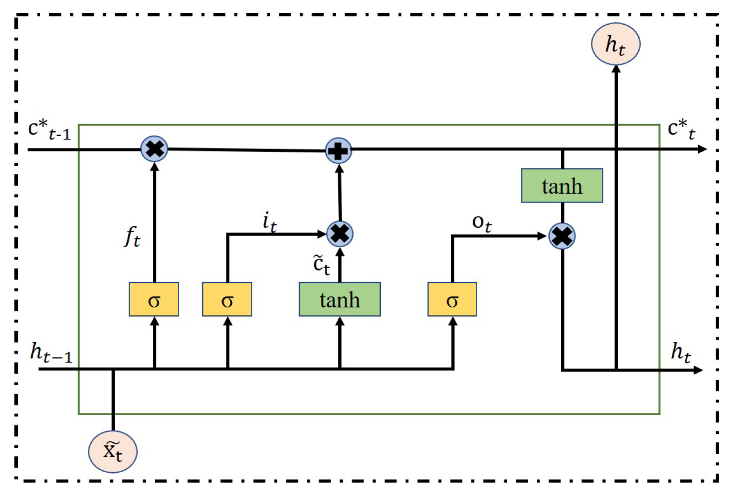
The new input sequence finally enters the LSTM network of the encoder part with different input variable information, and obtains the hidden state at time step t. The structure of LSTM is shown in Figure 3, and its definition can be expressed as:

$$\left\{\begin{array}{c}{f}_t=\sigma (w_f[h_{t-1},\widetilde{x_t}]+b_f)\\ i_t=\sigma (w_i[h_{t-1},\widetilde{x_t}]+b_i)\\ O_t=\sigma (w_o[h_{t-1},\widetilde{x_t}]+b_o)\\ \widetilde{c_t}=tanh(w_c[h_{t-1},\widetilde{x_t}]+b_c)\\ c_t^{*}=f_t·c_{t-1}^{\ast }+i_t·\widetilde{c_t}\\ h_t=O_t·tanh\left(c_t\right)\end{array}\right.$$

(8)

Moreover, the hidden state of the encoder part can be expressed as:

$$h_t=f_{LST{M}_1}(\widetilde{x_t},h_{t-1})$$

(9)

Subsequently, a temporal attention mechanism is introduced after the LSTM network of the encoder, which assigns a temporal attention weight to the hidden state in each LSTM network, as shown in Equation (10), and is weighted by the latter hidden states that adaptively determine the hidden states generated instantaneously by the encoder LSTM at all moments.

$$g_t^n=U_s^{2}tanh(W^{x2}{h}_t+W^{h2}{s}_{t-1}+b_2)$$

(10)

where $n\in [1,T]$, $U_s^2$, $W^{x2}$, $W^{h2}$ are the parameters that the network needs to learn through training, and the assignment of the temporal attention weight depends on the current input $h_t$ and the LSTM hidden variable $s_{t-1}$ from time step $t-1$. The non-linear function tanh is used as the activation function due to its good convergence performance. Then, ${\beta }_t^n$ is obtained after normalizing $g_t^n$:

$${\beta }_t^n=\frac{exp\left(g_t^n\right)}{{\sum }_{i=1}^{T}exp\left({\beta }_t^i\right)}$$

(11)

Calculating the hidden sequence and the temporal attention weight can finally obtain the changing intermediate vector $c_n$:

$$c_n=\sum _{t=1}^T{\beta }_t^n{h}_t$$

(12)

The LSTM hidden layer of the decoder part can be represented as:

$$s_n=f_{LST{M}_2}(y_{n-1},c_n,s_{n-1})$$

(13)

Finally, the predicted output $y_n$ is obtained from the intermediate vector $c_n$ and the hidden layer output $s_n$ updated by the decoder at moment $t=n$:

$$y_n=U_s^3(W^{w1}\langle s_n,c_n\rangle +b_3)$$

(14)

where $U_s^3$, $W^{w1}$ and $b_3$ are the model parameters that the neural network can learn.

3. Virtual Sensor Modeling Based on MIC-STALSTM

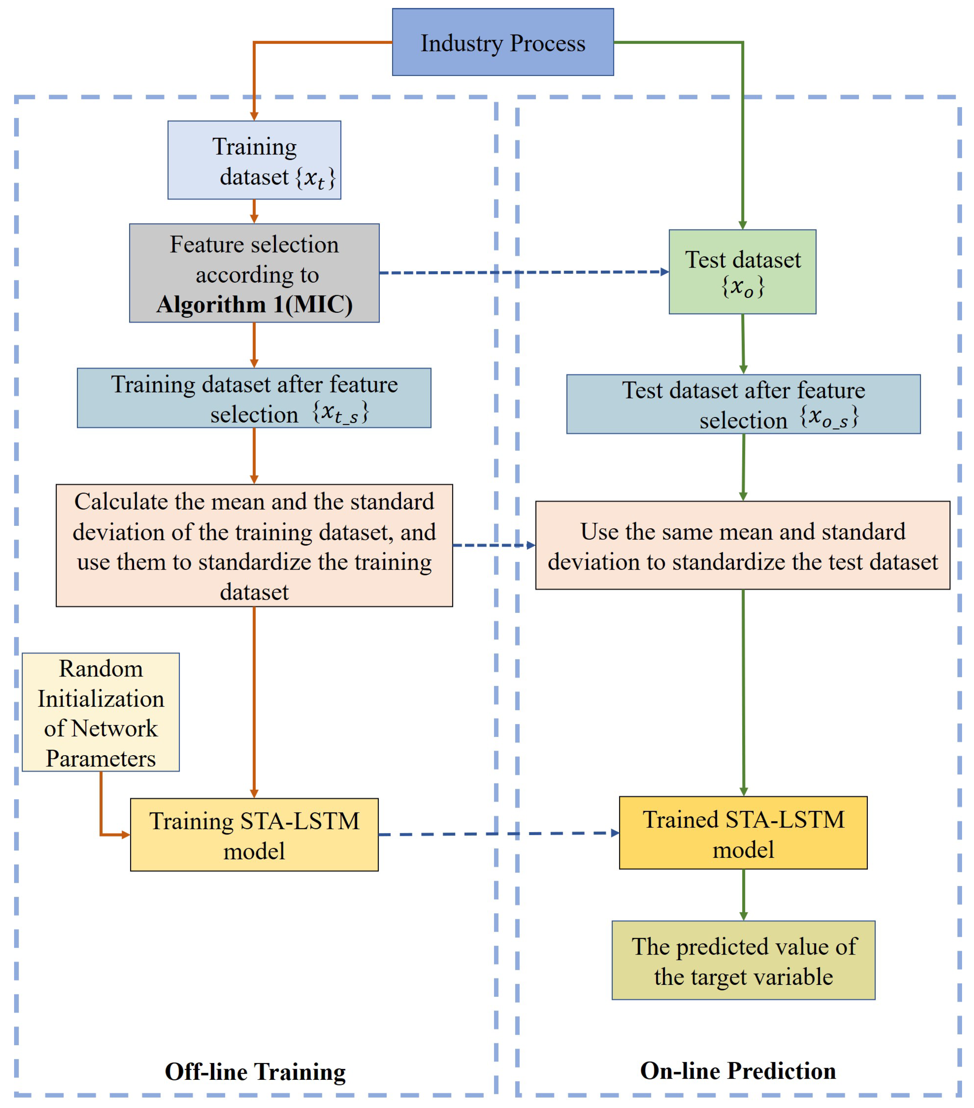
This section introduces the virtual sensor modeling process based on the MIC-STALSTM algorithm, and its framework is shown in Figure 4. In the following subsections, we will introduce the process of using the virtual sensor model to predict the temperature variables. The process includes offline training, online prediction, and evaluation of the prediction performance of the virtual sensors through three different indicators.

3.1. Offline Training

The dataset collected in an industrial process is divided into a training dataset $\left\{x_t\right\}$ and test dataset $\left\{x_o\right\}$. The detailed steps of the offline model training of MIC-STALSTM are shown below.

Step 1: Through Algorithm 1, perform feature selection on the training dataset $\left\{x_t\right\}$ to obtain the dataset $\left\{x_{t\_s}\right\}$;

Step 2: Normalize the dataset $\left\{x_{t\_s}\right\}$;

Step 3: Input the pre-processed training dataset and the network hyperparameter set in advance into the model to train the STA-LSTM model.

3.2. Online Prediction

When the training dataset obtains relatively satisfactory results and performance on the model MIC-STALSTM, the network parameters are saved and used for the online prediction of target variables. The steps are described as follows.

Step 1: Through the MIC value obtained from the training dataset, perform the same feature selection on the test dataset $\left\{x_o\right\}$ to obtain the dimension-reduced test dataset $\left\{x_{o\_s}\right\}$;

Step 2: Use the normalization parameter of $\left\{x_{t\_s}\right\}$ to normalize the test dataset $\left\{x_{o\_s}\right\}$;

Step 3: Place the test dataset after preprocessing into the trained STA-LSTM model to obtain the final prediction outputs.

Algorithm 1 Feature selection through maximal information coefficient

Input:  Discrete variables Output:  Variables after feature selection 1: Step1:Maximum mutual information 2: for each grid G do 3:     Explore the scatter plot for each grid 4:     Compute mutual information $MI\left(D\right|G)$ 5:     $M{I}^{\ast }(D,i,j)\leftarrow MI\left(D\right|G)$ 6: end for 7: Step2:Normalization 8: Normalization of $M{I}^{\ast }(D,i,j)$, $0\le M{I}^{\ast }(D,i,j)\le lo{g}_2\left(min(i,j)\right)$ 9: Step3:MIC 10: Calculate MIC with limits: $i\times j<B\left(n\right)\cap B\left(n\right)=n^{0.6}$ 11: Step4:Feature selection 12: for each MIC do 13:     $MIC\ge Athreshold$ 14: end for

3.3. Performance Indicators

The prediction performance of the model is evaluated by three indicators: root mean square error (RMSE), mean absolute value error (MAE), and coefficient of determination ($R^2$). The root mean square error (RMSE) and mean absolute value error (MAE) are defined as follows:

$$RMSE=\sqrt{\frac{1}{N}\sum _{i=1}^n\frac{y_i-\widehat{y_i}}{y_i}}$$

(15)

$$MAE=\frac{1}{N}\sum _{i=1}^N|y_i-\widehat{y_i}|$$

(16)

In the above two equations, N is the total number of training samples, $y_i$ is the true value of the test data, and $\widehat{y_i}$ is the predicted value of the data output by the model. Among them, RMSE focuses on calculating the prediction error of the entire test dataset according to the above definition. Furthermore, MAE can also better reflect the real situation of the predicted value error. This is because the errors are absolute values, and there is no situation where positive and negative errors cancel each other out. It can be seen from the definitions of RMSE and MAE that the smaller the values of RMSE and MAE, the smaller the model prediction error and the more accurate the prediction. Moreover, another indicator that is widely used in forecasting problems is the coefficient of determination $R^2$, which is defined as follows:

$$R^2=1-\frac{{\sum }_{i=1}^N{(y_i-\widehat{y_i})}^2}{{\sum }_{i=1}^N{(y_i-\overline{y})}^2}$$

(17)

where $\overline{y}$ represents the average of all training samples. $R^2$ represents the squared correlation between the true and predicted outputs. With $R^2$ being closer to 1, better predictive performance of the model is indicated.

4. Case Study

In this section, the working principle of the HVAC system and the dataset used for the algorithm performance comparison are described in detail. Moreover, the performance of the proposed MIC-STALSTM algorithm is validated for the prediction of two temperature variables in the HVAC system. The two temperature variables are the chilled water return temperature variable $T_{chwr}$ and the chilled water supply temperature variable $T_{chws}$. For $T_{chwr}$, we aim at demonstrating the effectiveness of the MIC-STALSTM when there are switches in operating conditions in the HVAC system. For $T_{chws}$, the superiority of MIC-STALSTM is verified when there is no work switching in the HVAC system.

4.1. Description of HVAC Systems

4.1.1. The Working Principles of HVAC Systems

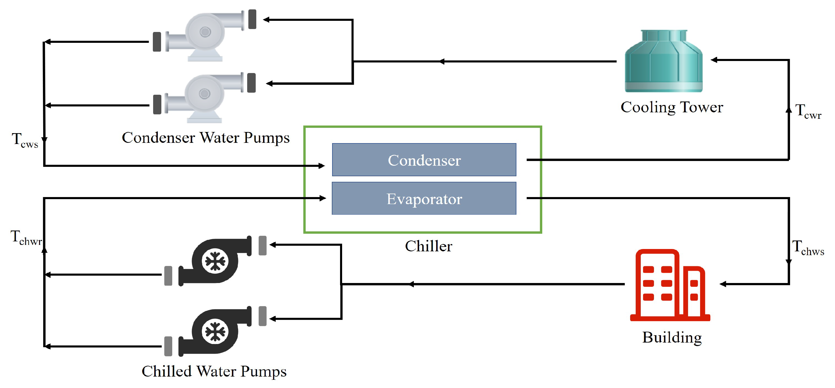
Figure 5 gives the basic working principle of a heating, ventilation, and air-conditioning (HVAC) system that contains two heat exchange circulation systems, internal and external circulation. In the internal circulation (bottom half of Figure 5), chilled water pumps push $T_{chws}$ cold water cooled by a chiller into the building to cool and dehumidify the air inside the building through heat exchange. The circulating water, which has absorbed the heat of the air inside the building and increased in temperature to $T_{chwr}$, is returned to the chiller for cooling, and its heat is transferred to the external circulation via the condenser. In the external circulation (top half of Figure 5), the condenser water pumps drive the water in the condenser to absorb the heat generated by the evaporator to the cooling tower, which discharges the heat from the water to the outdoor air, where it flows back to the condenser and so on. The evaporator in the internal circulation and the condenser in the external circulation are encapsulated together, and this whole is known as the chiller. The HVAC system absorbs the heat from the indoor environment and transports it to the outdoors through energy conversion, so as to achieve air exchange and cooling.

4.1.2. Data Description

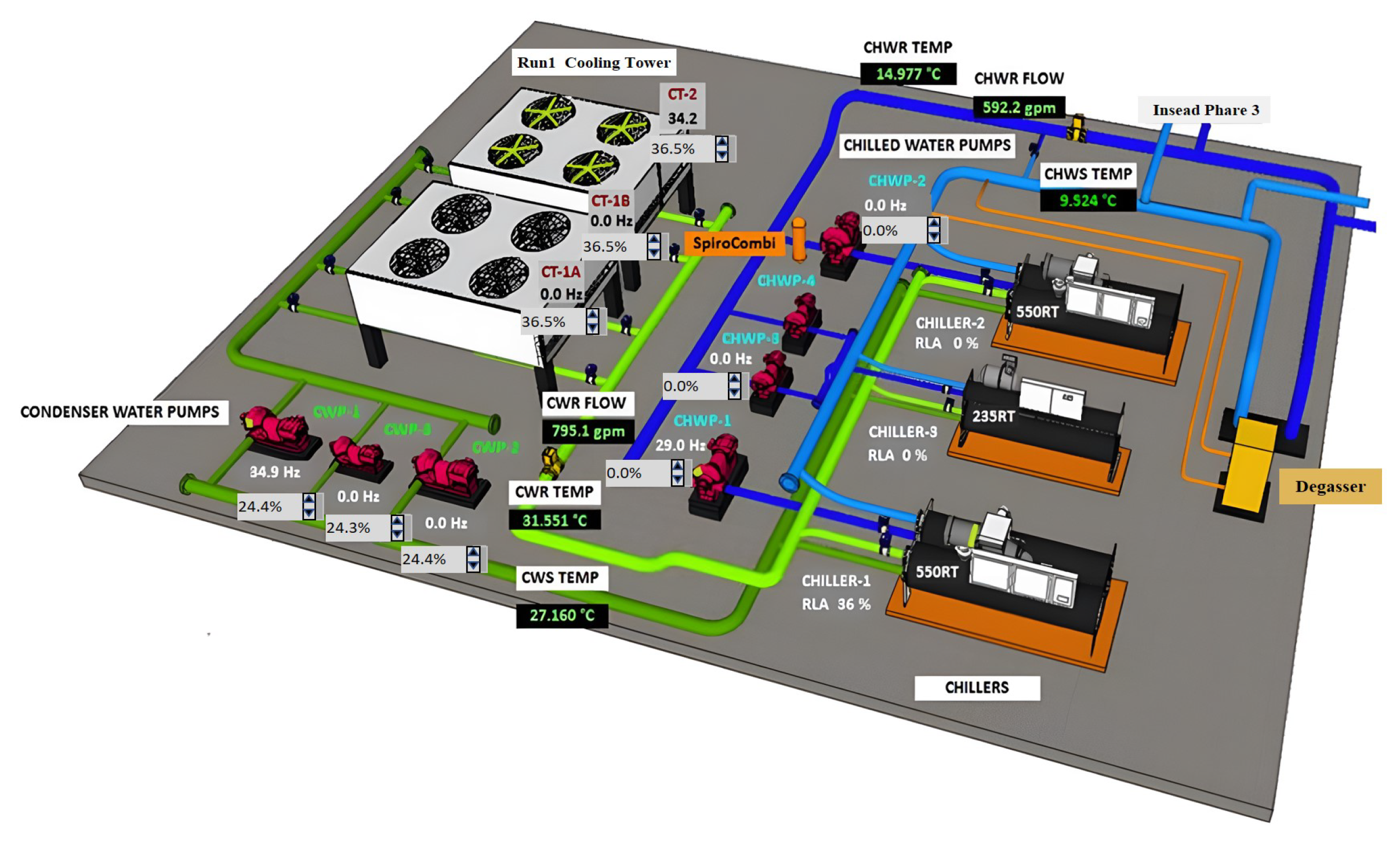
The HVAC system selected for analysis is applied to the space cooling of a high-rise office building located in a city in the tropical region of China. The city’s annual average temperature is in the range of 25–32 °C, and the average humidity is around 85%. Figure 6 presents the schematic of the HVAC system, which employs three chillers, two cooling towers, three condenser water pumps, and four chilled water pumps. The three chillers are rated at 550 RT, 550 RT, and 235 RT, respectively (RT is the cooling tonne, i.e., a unit of power indicating cooling capacity, 1RT = 3.517 kW).

The overall dataset was sampled from the operational data of the HVAC system at the actual site from 0:00 on 30 January 2017 to 23:13 on 14 February 2017, with a total sampling duration of 16 days. The sampling interval was 1 min and data were collected for a total of 50 parameters, with detailed parameters’ descriptions shown in

Table 1. The description of the HVAC system parameters.

No.	Variables	Descriptions	Unit
1	RH	Relative humidity	%
2	$T_{dryb}$	Dry bulb temperature	°C
3	$T_{wetb}$	Wet bulb temperature	°C
4	$S_{ch1}$	Status of the chiller No. 1
5	$S_{ch2}$	Status of the chiller No. 2
6	$S_{ch3}$	Status of the chiller No. 3
7	$P_{ch1}$	Power of the chiller No. 1	kW
8	$P_{ch2}$	Power of the chiller No. 2	kW
9	$P_{ch3}$	Power of the chiller No. 3	kW
10	${\eta }_{chiller\_eff}$	Efficiency of the chiller	kW/RT
11	$S_{chwp1}$	Status of chilled water pump No. 1
12	$S_{chwp2}$	Status of chilled water pump No. 2
13	$S_{chwp3}$	Status of chilled water pump No. 3
14	$S_{chwp4}$	Status of chilled water pump No. 4
15	$P_{chwp1}$	Power of chilled water pump No. 1	kW
16	$P_{chwp2}$	Power of chilled water pump No. 2	kW
17	$P_{chwp3}$	Power of chilled water pump No. 3	kW
18	$P_{chwp4}$	Power of chilled water pump No. 4	kW
19	$M_{chwp\_pc}$	Speed of chilled water pump	%
20	$T_{chws}$	The temperature of water flowing out of the chiller	°C
21	$T_{dch}$	Cooling effect: temperature difference between $T_{chws}$ and $T_{chwr}$	°C
22	$v_{chwsfhdr}$	The flow rate of cooling water in internal circulation	gal/min
23	$v_{chwgpmrt}$	Load flow rate: $v_{chwsfhdr}$/$L_{sys}$	gal/min·RT
24	$S{P}_{chwgpmrt}$	Setting point of $v_{chwgpmrt}$	gal/min·RT
25	$S_{cwp1}$	Status of condenser water pump No. 1
26	$S_{cwp2}$	Status of condenser water pump No. 2
27	$S_{cwp3}$	Status of condenser water pump No. 3
28	$P_{cwp1}$	Power of condenser water pump No. 1	kW
29	$P_{cwp2}$	Power of condenser water pump No. 2	kW
30	$P_{cwp3}$	Power of condenser water pump No. 3	kW
31	$n_{cwp\_pc}$	Rate of condenser water pump	%
32	${\eta }_{cwp\_eff}$	Average efficiency of condenser water pump	kW/RT
33	$T_{cwr}$	The temperature of the water flowing out of the condenser	°C
34	$T_{cws}$	The temperature of the water flowing into the condenser	°C
35	$v_{cwsfhdr}$	The flow rate of chilled water in external circulation	gal/min
36	$v_{cwgpmrt}$	Load flow rate: $v_{cwsfhdr}$/$L_{sys}$	gal/min·RT
37	$S{P}_{cwgpmrt}$	Setting point of $v_{cwgpmrt}$	gal/min·RT
38	$S_{ct1}$	Status of cooling tower No. 1
39	$S_{ct2}$	Status of cooling tower No. 2
40	$P_{ct1}$	Power of cooling tower 1	kW
41	$P_{ct2}$	Power of cooling tower 2	kW
42	$M_{ct\_pc}$	Speed of cooling tower fans	%
43	${\eta }_{ct\_eff}$	Average efficiency of cooling tower	kW/RT
44	$S{P}_{ct\_eff}$	Setting point of ${\eta }_{ct\_eff}$	kW/RT
45	$Q_{systp}$	Power consumption of the total system	kW
46	$L_{sys}$	The cooling load of the total system	RT
47	${\eta }_{effsys}$	Efficiency of the total system	kW/RT
48	$H{B}_{sys}$	Thermal balance of the total system	%
49	${\eta }_{chwp\_eff}$	Average efficiency of chilled water pumps	kW/RT
50	$T_{chwr}$	The temperature of the water flowing into the chiller	°C

. Emphasis needs to be placed on the fact that the values taken for all HVAC parameters are point data and not the averaged data over 1 min. A total of 18,292 samples were stored during the sampling process and the overall sample dataset was divided into two separate data subsets, a training dataset containing 5000 sample points and a test dataset containing 13,292 sample points. At the same time, the HVAC system has the characteristic of operating under variable conditions over a long period of time, and this characteristic is reflected in the dataset. At sample point 6125, the change in state of variables $S_{chwp1}$ and $S_{chwp2}$ triggers a change in condition from chilled water pump No. 1 to chilled water pump No. 2, which continues until sample point 9965. At sample point 9665, chilled water pump No. 2 switches to chilled water pump No. 1 again. Similarly, at sample points 12,885 and 14,910, the increase in the state variables $n_{cwp\_pc}$ and $M_{chwp\_pc}$ leads to a change in the flow rate and an increase in the head of the condenser and chilled water pumps.

4.2. MIC-STALSTM for Temperature Prediction

4.2.1. Pre-Processing of Variables in the HVAC System by MIC

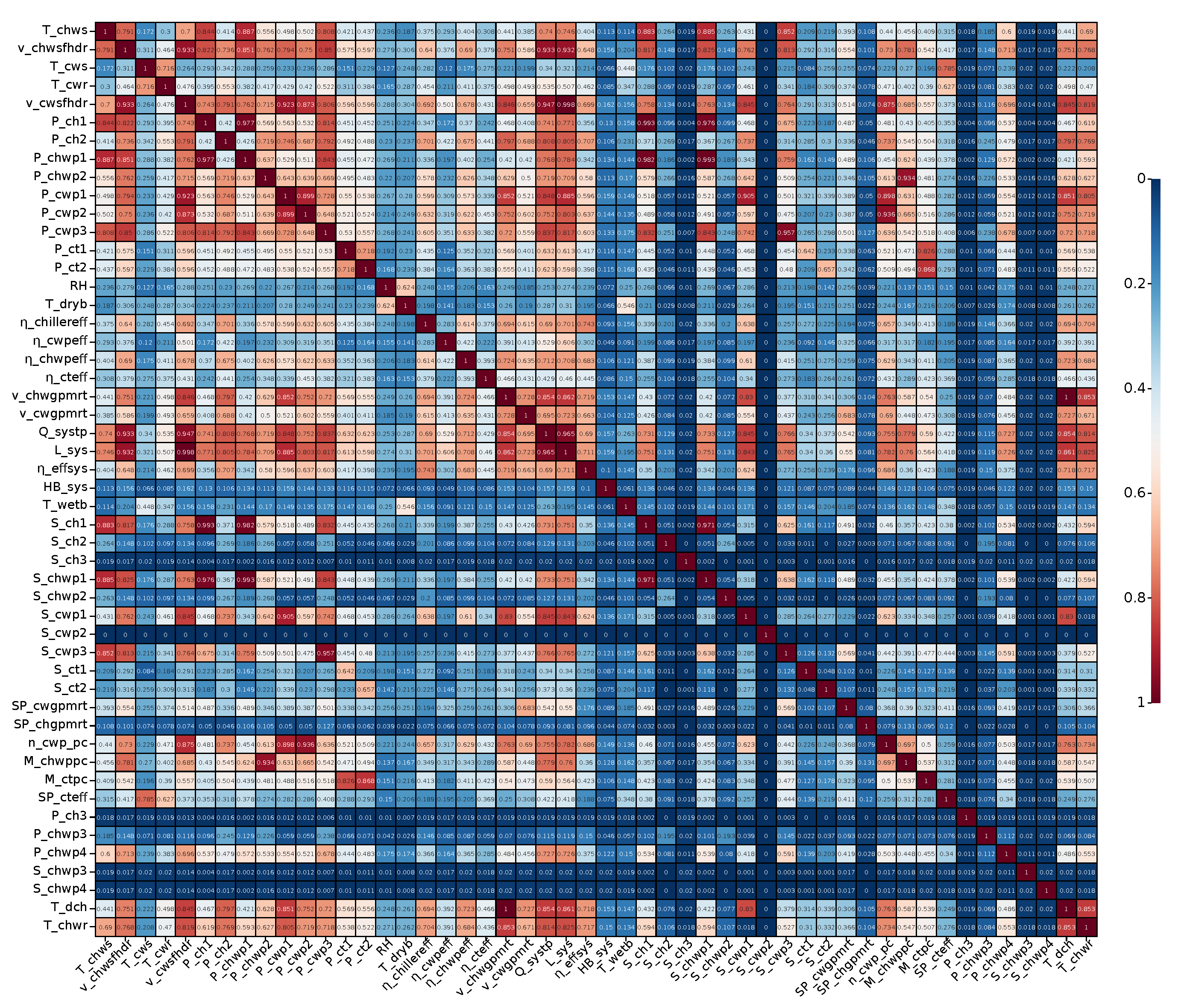
Due to the complex coupling between variables in the HVAC system, inputting all variables into the prediction model at the same time can easily lead to problems such as duplication of information and invalid features. These problems may have a negative impact on the accuracy of the virtual sensor model. Moreover, the 50 variables involved in the HVAC system are frequently faced with switching conditions, which can lead to drastic changes in sensor values. Sudden changes in sensor values can also have a significant impact on model accuracy. For the purpose of solving the above two problems and further improving the prediction accuracy of the virtual sensors, MIC values were calculated in order to prepare for subsequent variable selection. Figure 7 shows the coefficient matrix calculated by MIC, and the values in the coefficient matrix represent the MIC metric between the variables two by two in the HVAC system.

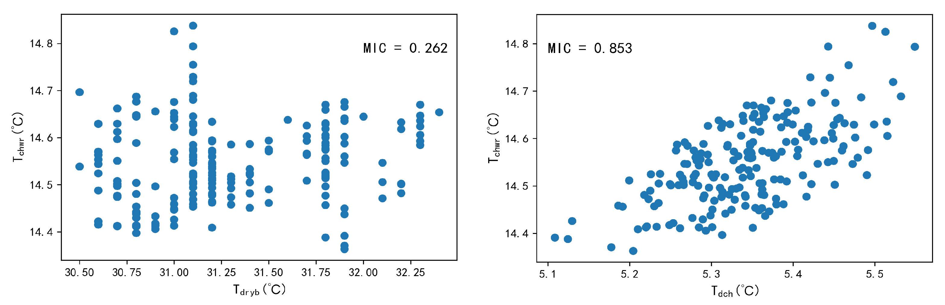
In order to verify that the relationships between the variables corresponding to different MIC values are significantly different, Figure 8 shows the scatter plots between the dry bulb temperature $T_{dryb}$ and the return water temperature $T_{chwr}$; the cooling effect $T_{dch}$ and the return water temperature $T_{chwr}$. As can be seen in Figure 8, $T_{dryb}$ and $T_{chwr}$, whose MIC vaule is equal to 0.262, are independent of each other. Moreover, there is a linear correlation between $T_{dch}$ and $T_{chwr}$ for an MIC value equal to 0.853, although there are a few outliers due to variations in operating conditions and loads. The larger the MIC value, the higher the correlation between the variable and the target variable, and the more information about the target variable it contains. Therefore, by choosing an MIC value greater than a certain threshold, it is ensured that the feature variables selected for prediction remain highly correlated with the target variables. Ultimately, the threshold for MIC was determined to be 0.7 based on empirical selection [21]. For $T_{chwr}$, 11 variables with MIC values greater than 0.7 were selected as the input feature variables, as shown in Equation (18). For $T_{chws}$, 10 variables were selected as the input feature variables, as shown in Equation (19).

$$T_{chwr}=f(P_{ch2},P_{cwp1},P_{cwp2},P_{cwp3},{\eta }_{chiller\_eff},v_{chwsfhdr},T_{dch},v_{chwgpmrt},Q_{systp},L_{sys},{\eta }_{effsys})$$

(18)

$$T_{chws}=f(v_{chwsfhdr},v_{cwsfhdr},P_{ch1},P_{chwp1},P_{cwp3},Q_{systp},L_{sys},S_{ch1},S_{chwp1},S_{cwp3})$$

(19)

4.2.2. The Selection of Hyperparameters of STA-LSTM

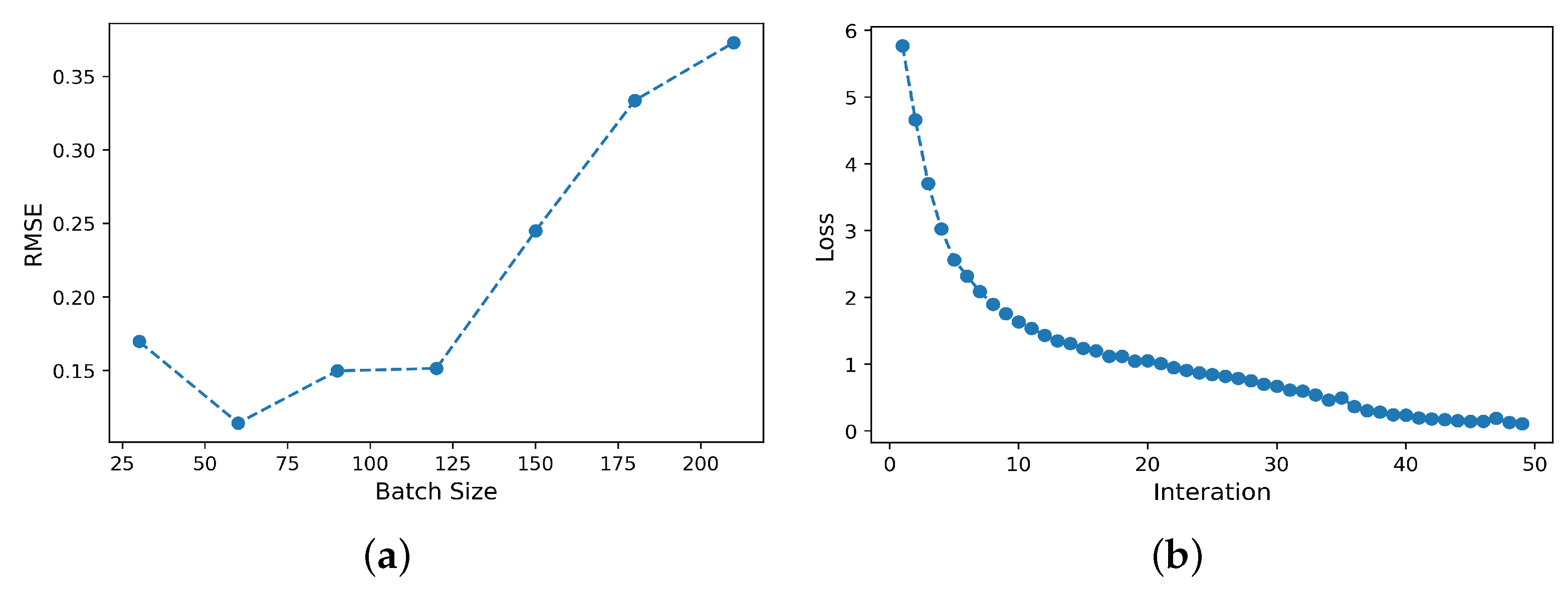
After pre-processing the variables in the HVAC system by MIC, the filtered variables are used as feature variables for the training and prediction of the STA-LSTM network. Then, for STA-LSTM, several hyperparameters in the algorithm need to be determined rationally in order to achieve high accuracy. Some of the most commonly used methods for determining hyperparameters include trial and error, grid search, random search, and Bayesian optimization. For the STA-LSTM studied in this paper, the hyperparameters to be optimized include batch size, the number of neurons, and iterations, etc. In this paper, the optimal set of parameters is confirmed by a combination of random search and trial and error. Firstly, by randomly generating several different sets of hyperparameters to obtain different experimental results, the approximate optimal interval is gradually found. Subsequently, the detailed optimal parameter set is found by the trial and error method. For $T_{chwr}$, different batches in the range [30, 60, 90, 120, 150, 180, 210] show the performance trend of the STA-LSTM-based virtual sensor model. As shown in Figure 9a, with the increase in the batch size, the general trend of RMSE first decreases and then moves upwards, and remains relatively stable. The appropriate batch size should preferably be set between 30 and 90. In this paper, it is set to 64. As another important hyperparameter, the number of iterations is set to 50. At this number of iterations, the loss function of the STA-LSTM network converges on the training dataset, as shown in Figure 9b.

All of the neural network models used in this paper have approximately the same structure. Therefore, the neural network models were all placed under the same hyperparameters for training, which helps to compare the differences between the different models. Similar to the method for determining the batch size, the hyperparameters used for all algorithms were finally determined, as shown in

Table 2. The final values of the hyperparameters corresponding to different target variables.

Method	Learning Rate	Hidden Unit	Batch Size	Time Step	Iterations
$T_{chwr}$	0.001	60	64	4	50
$T_{chws}$	0.003	60	64	3	50

.

4.2.3. Performance Comparison

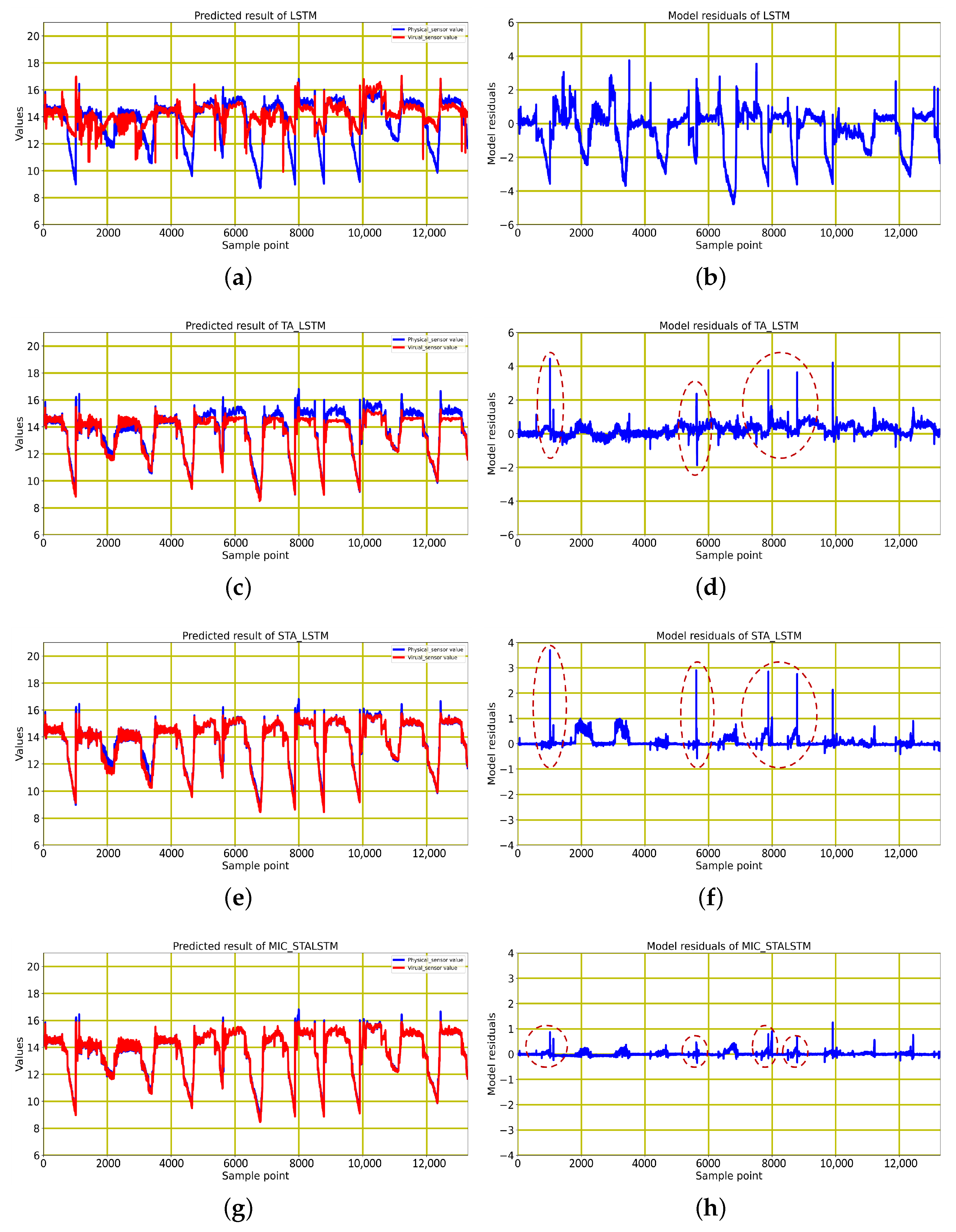
To demonstrate the effectiveness of combining MIC with STA-LSTM, the algorithm of MIC-STALSTM is used with LSTM, TA-LSTM, and STA-LSTM for the predictions of the temperature variable $T_{chwr}$ on the test dataset, as shown in Figure 10. Moreover, in Figure 10, the model deviation corresponding to each model for the temperature prediction is given. In the prediction images corresponding to the four algorithms, the red solid line denotes the predicted value given by the virtual sensor, and the blue solid line denotes the true value of the actual hardware sensor. It can be seen that large deviations exist between the predicted and actual curves for LSTM. The predicted curve of the TA-LSTM-based model can roughly track the trend of the actual curve. Then, the prediction curve of the virtual sensor based on the STA-LSTM algorithm is more closely aligned with the blue curve of the actual sensor value compared with the previous two algorithms. However, from the area circled by the red dotted line in Figure 10f, it can be seen that the predictions of the STA-LSTM-based model at some fixed sampling points still have large prediction errors, such as at sample point 1125, at sample point 4665, at sample point 7885, and at sample point 9910 in the test data. These coarse prediction errors are caused by the switching among different operating conditions in the HVAC system.

In general, the attention-based TA-LSTM and STA-LSTM are able to adjust the influence of different input variables on the target variable by adaptively adjusting the weights to ensure the accuracy of prediction. However, due to the abruptness of the HVAC system’s operating condition transitions, the attention-based TA-LSTM and STA-LSTM are unable to adjust the weights to accurately predict the target temperature variable $T_{chwr}$ in a timely manner. Therefore, the predicted values of the virtual sensors are inaccurate compared to the measured values of the actual sensors. In contrast, the improved MIC-STALSTM algorithm first extracts the influences highly correlated with $T_{chwr}$ by MIC before proceeding with the virtual sensor modeling. As can be seen in Equation (18), the variables that have an impact on the operating conditions at the four sampling points, $S_{chwp1}$, $S_{chwp2}$, $n_{cmp\_pc}$, and $M_{chwp\_pc}$, are not among the filtered feature variables. Thus, by displaying the area outlined by the red dotted line in Figure 10h, the MIC-STALSTM algorithm is more accurate in predicting the variable $T_{chwr}$ at the four sampling points of the work condition switch.

The MAE, RMSE, and $R^2$ of the four different algorithms for the variable $T_{chwr}$ on the test dataset are given in

Table 3. Prediction performance indicators of the four algorithms for the variable $T_{chwr}$.

Method	MAE	RMSE	${\mathit{R}}^2$
LSTM	0.9029	1.3146	0.3185
TA-LSTM	0.2951	0.3940	0.9387
STA-LSTM	0.0969	0.2340	0.9784
MIC-STALSTM	0.0415	0.0758	0.9977

. As can be seen from Table 3, LSTM has the worst prediction performance, with the largest MAE and RMSE and the smallest $R^2$ metrics among the four algorithms. With the feature selection of the dataset by MIC and the introduction of the spatial–temporal attention mechanism, MIC-STALSTM is able to capture the data features and information in the industrial time series more effectively. It provides the best prediction accuracy of the four algorithms, as evidenced by the smallest values of the MAE and RMSE metrics and the largest values of the $R^2$.

At the same time, as there are 50 variables involved in the HVAC system, too many input variables or the presence of covariance may have a negative impact on the model accuracy. Since MIC-STALSTM is capable of filtering highly correlated characteristic variables by MIC, its prediction performance is better than the LSTM, TA-LSTM, and STA-LSTM algorithms even without the conditional switching problem. To further validate the superior performance of MIC-STALSTM, the states of the variables are modified in the dataset. The four sample points for the switching of operating conditions described before no longer switch, and continue to maintain the original state at the previous moment. For example, at sample point 1125 of the test data, instead of switching from chilled water pump No. 1 to chilled water pump No. 2, the condition of chilled water pump No. 1 is maintained.

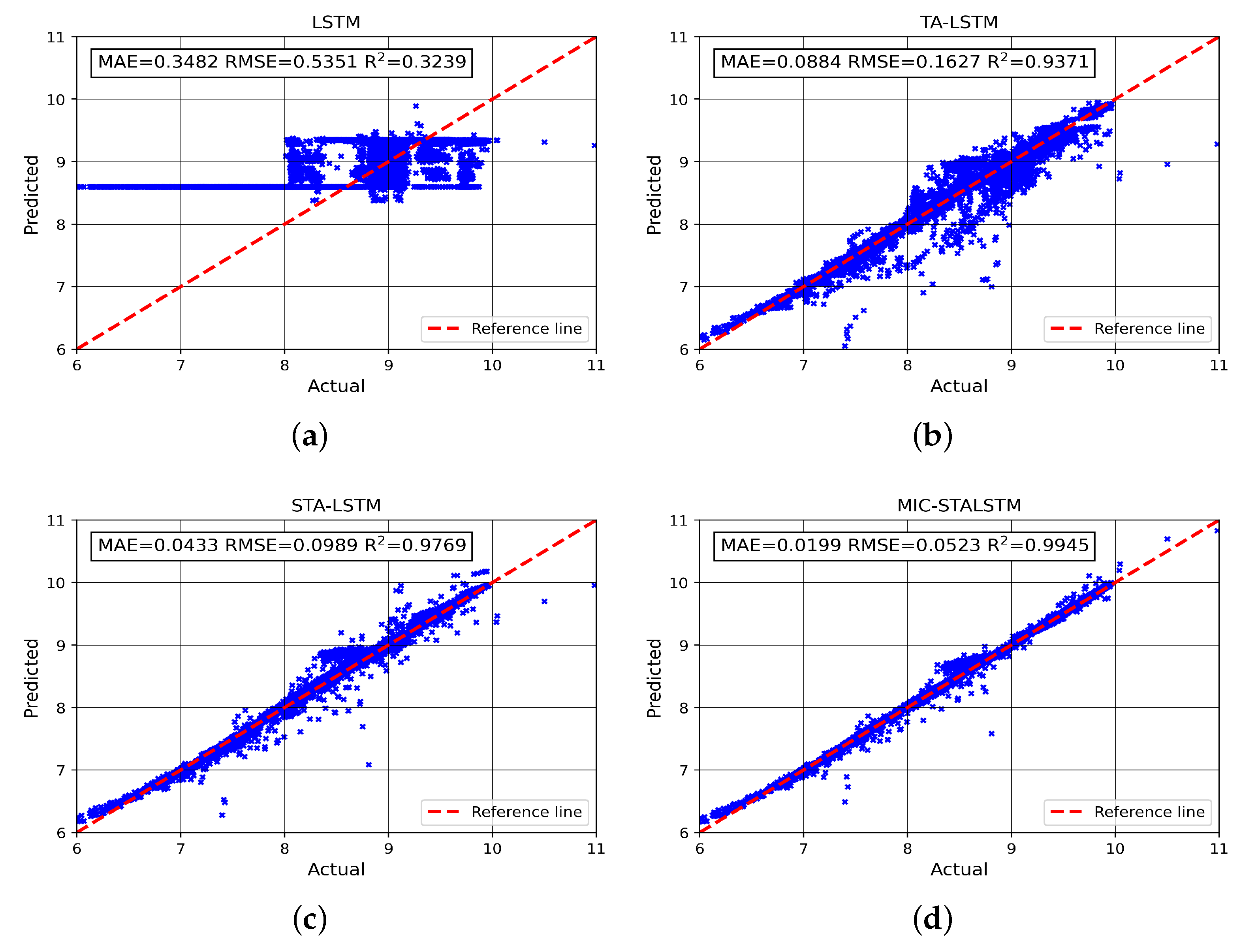
For $T_{chws}$, the prediction results of the four different algorithms without frequent switching of operating conditions are shown in Figure 11. In Figure 11, the horizontal axis is the labeled value and the vertical axis is the predicted value. The closer the scatter is to the main diagonal (red reference line), the better the prediction performance. Thus, the MIC-STALSTM shows the best prediction for $T_{chws}$ compared to the other three algorithms, because the scatter distribution of MIC-STALSTM is more concentrated near the main diagonal line throughout the prediction interval $[6,11]$.

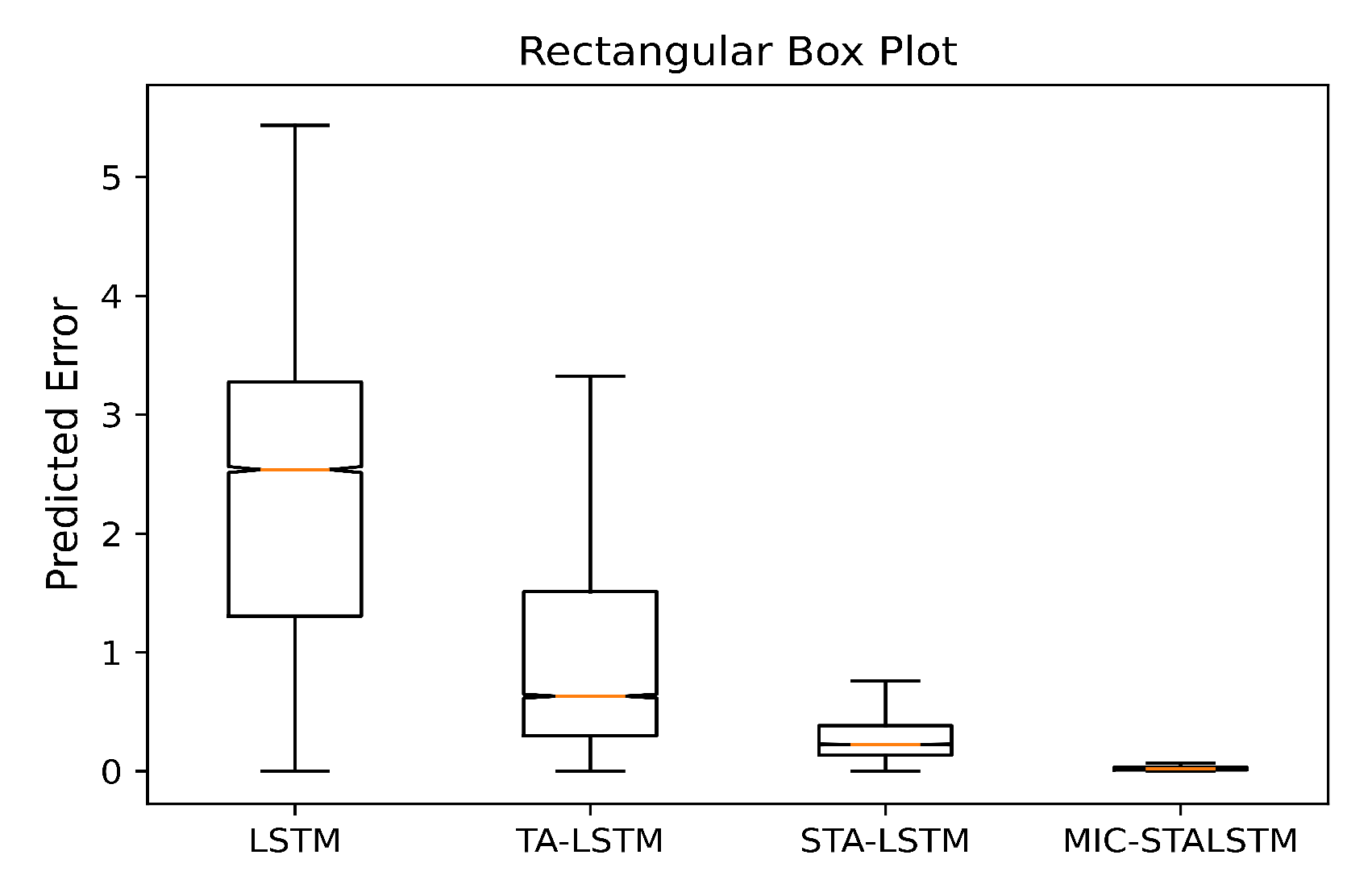
In order to show more intuitively the prediction performance of the four different algorithms for the target variable $T_{chws}$, box plots of the absolute prediction errors for the four methods are given in Figure 12, which can effectively reflect the data distribution characteristics of the absolute errors. In each box plot, the medians of the absolute prediction errors are indicated by the orange markers in the boxes. Moreover, the bottom and top of the box, respectively, represent the lower and upper quartiles of the absolute error of the different algorithms. In addition, the normal distribution parameters for the four algorithms and the $\mu \pm 3\sigma$ intervals corresponding to the different normal distribution parameters are presented in

Table 4. Confidence intervals’ prediction error.

Parameter	LSTM	TA-LSTM	STA-LSTM	MIC-STALSTM
$\mu$	2.2743	1.1471	0.3319	0.0299
$\sigma$	1.1468	1.2216	0.3500	0.0445
$[\mu -3\sigma ,\mu +3\sigma ]$	$[-1.1661,5.7147]$	$[-2.5177,4.8119]$	$[-0.7181,1.3819]$	$[-0.1036,0.1634]$

. From Figure 12 as well as from Table 4, it can be seen that the prediction errors of MIC-STALSTM are more densely distributed around 0 and have the narrowest confidence intervals $[\mu -3\sigma ,\mu +3\sigma ]$.

Therefore, when there is no frequent switching of operating conditions in the HVAC system, MIC-STALSTM still achieves a further improvement in prediction accuracy for the temperature variable $T_{chws}$ compared to the remaining three algorithms.

5. Conclusions

This paper mainly presents a virtual sensor modeling method for the temperature of supply and return water at both ends of the chiller in an HVAC system. The traditional STA-LSTM algorithm can adaptively adjust spatial attention to change the corresponding weights of different input variables at different time steps. Moreover, it is capable of adjusting the temporal attention to change the temporal correlation of the hidden state of the neural network. However, the model based on STA-LSTM is not suitable for the target variable prediction of the HVAC system, which is due to the following problems in virtual sensor modeling in HVAC systems: (1) not all variables contribute positively to the modeling of virtual sensors, due to the complex coupling between variables; (2) the total HVAC system is constantly faced with changes in system conditions and operating loads, which will lead to sudden changes in different variables. The weight adaptive adjustment of STA-LSTM cannot work well under a sudden change in working conditions. At the sample points with sudden changes in operating conditions, the virtual sensor model established by the STA-LSTM algorithm has a large prediction error. Therefore, based on the deficiency of the STA-LSTM algorithm and the operational characteristics of HVAC systems, this paper proposes an MIC-STALSTM algorithm that combines MIC and STA-LSTM, which screens out the influence factors with low correlations with the target temperature variable by MIC. When the filtered influence factor is used as the main variable leading to the change in working conditions, the prediction of the temperature variable by the MIC-STALSTM algorithm will no longer be affected by the auxiliary variable. Using the MIC-STALSTM-based virtual sensor to accurately model the $T_{chwr}$ temperature shows that the MIC-STALSTM is a suitable modeling method when the system is faced with a change in operating conditions. At the same time, since MIC performs feature extraction on a large number of features in the original dataset, the input variables involved in subsequent prediction are highly correlated with the target variables. By establishing a virtual sensor for the supply water temperature variable $T_{chws}$ of the chiller, it is verified that the prediction performance of MIC-STALSTM is more precise and effective than the other three algorithms without facing frequent switching conditions in the HVAC system.

This paper provides a comprehensive overview of the MIC-STALSTM-based approach to virtual sensor modeling. However, it has a limitation in which the modeling framework does not depart from the basic virtual sensor framework (i.e., offline training and online prediction), which makes the model completely fixed in the process of online prediction. The completely fixed model may suffer from a degradation in predictive performance for time-varying HVAC systems. For further work, more attention will be paid to online adaptive modeling for virtual sensors.

References

- Reppa, V.; Papadopoulos, P.; Polycarpou, M.M.; Panayiotou, C.G. A Distributed Architecture for HVAC Sensor Fault Detection and Isolation. IEEE Trans. Control Syst. Technol. 2014, 23, 1323–1337. [Google Scholar] [CrossRef] [Green Version]
- Choi, Y.; Yoon, S. Virtual sensor-assisted in situ sensor calibration in operational HVAC systems. Build. Environ. 2020, 181, 107079–107090. [Google Scholar] [CrossRef]
- Sedghi, S.; Sadeghian, A.; Huang, B. Mixture semisupervised probabilistic principal component regression model with missing inputs. Comput. Chem. Eng. 2017, 103, 176–178. [Google Scholar] [CrossRef]
- Chen, J.; Yang, C.; Zhou, C.; Li, Y.; Zhu, H.; Gui, W. Multivariate Regression Model for Industrial Process Measurement Based on Double Locally Weighted Partial Least Squares. IEEE Trans. Instrum. Meas. 2020, 69, 3962–3971. [Google Scholar] [CrossRef]
- Desai, K.; Badhe, Y.; Tambe, S.S.; Kulkarni, B.D. Soft-sensor development for fed-batch bioreactors using support vector regression. Biochem. Eng. J. 2006, 27, 225–239. [Google Scholar] [CrossRef]
- Kusiak, A.; Li, M.; Zheng, H. Virtual models of indoor-air-quality sensors. Appl. Energy 2010, 87, 2087–2094. [Google Scholar] [CrossRef]
- Lin, T.; Pan, Y.; Xue, G.; Song, J.; Qi, C. A Novel Hybrid Spatial-Temporal Attention-LSTM Model for Heat Load Prediction. IEEE Access 2020, 8, 159182–159195. [Google Scholar] [CrossRef]
- Noor, F.; Haq, S.; Rakib, M.; Ahmed, T.; Jamal, Z.; Siam, Z.S.; Hasan, R.T.; Adnan, M.S.; Dewan, A.; Rahman, R.M. Water Level Forecasting Using Spatiotemporal Attention-Based Long Short-Term Memory Network. Water 2022, 14, 612. [Google Scholar] [CrossRef]
- Song, S.; Lan, C.; Xing, J. Spatio-Temporal Attention-Based LSTM Networks for 3D Action Recognition and Detection. IEEE Trans. Image Process 2018, 27, 3459–3471. [Google Scholar] [CrossRef] [PubMed]
- Feng, L.; Zhao, C.; Sun, Y. Dual Attention-Based Encoder-Decoder: A Customized Sequence-to-Sequence Learning for Soft Sensor Development. IEEE Trans. Neur. Net. Lear 2021, 32, 3306–3317. [Google Scholar] [CrossRef] [PubMed]
- Sun, Q.; Ge, Z. Gated Stacked Target-Related Autoencoder: A Novel Deep Feature Extraction and Layerwise Ensemble Method for Industrial Soft Sensor Application. IEEE Trans. Cybern. 2020, 52, 3457–3468. [Google Scholar] [CrossRef] [PubMed]
- Yuan, X.; Rao, J.; Gu, Y.; Ye, L.; Wang, K.; Wang, Y. Online Adaptive Modeling Framework for Deep Belief Network-Based Quality Prediction in Industrial Processes. Ind. Eng. Chem. Res. 2021, 60, 15208–15218. [Google Scholar] [CrossRef]
- Ke, W.; Huang, D.; Yang, F.; Jiang, Y. Soft Sensor Development and Applications Based on LSTM in Deep Neural Networks. In Proceedings of the 2017 IEEE Symposium Series on Computational Intelligence(SSCI), Honolulu, HI, USA, 27 November–1 December 2017. [Google Scholar]
- Yuan, X.; Li, L.; Wang, Y. Nonlinear Dynamic Soft Sensor Modeling With Supervised Long Short-Term Memory Network. IEEE Trans. Ind. Informat 2020, 16, 3168–3176. [Google Scholar] [CrossRef]
- Yuan, X.; Li, L.; Wang, Y.; Yang, C.; Gui, W. Deep learning for quality prediction of Nonlinear Dynamic Processes with Variable Attention-Based Long Short-Term Memory Network. Can. J. Chem. Eng. 2019, 98, 1377–1389. [Google Scholar] [CrossRef]
- Guo, Z.; Yu, B.; Hao, M.; Wang, W.; Jiang, Y.; Zong, F. A novel hybrid method for flight departure delay prediction using Random Forest Regression and Maximal Information Coefficient. Aerosp. Sci. Technol. 2021, 116, 106822–106832. [Google Scholar] [CrossRef]
- Reshef, D.N.; Reshef, Y.A.; Finucane, H.K.; Grossman, S.R.; McVean, G.; Turnbaugh, P.J.; Lander, E.S.; Mitzenmacher, M.; Sabeti, P.C. Detecting Novel Associations in Large Data Sets. Science 2011, 334, 1518–1524. [Google Scholar] [CrossRef] [PubMed] [Green Version]
- Wang, Y.; Yan, X. Soft Sensor Modeling Method by Maximizing Output-Related Variable Characteristics Based on a Stacked Autoencoder and Maximal Information Coefficients. Int. J. Comput. Intell. Syst. 2019, 12, 1062–1074. [Google Scholar] [CrossRef] [Green Version]
- Yuan, X.; Li, L.; Shardt, Y.A.; Wang, Y.; Yang, C. Deep Learning With Spatiotemporal Attention-Based LSTM for Industrial Soft Sensor Model Development. IEEE Trans. Ind. Electron. 2021, 68, 4404–4414. [Google Scholar] [CrossRef]
- Official of TipDM Cup, China. Available online: https://www.tipdm.org/u/cms/www/201703/09223534dgbb.pdf (accessed on 8 March 2017).
- Gao, L.; Li, D.; Li, D.; Yao, L.; Liang, L.; Gao, Y. A Novel Chiller Sensors Fault Diagnosis Method Based on Virtual Sensors. Sensors 2019, 19, 3013. [Google Scholar] [CrossRef] [PubMed] [Green Version]
Figure 1.
Some basic structures. (a) Structure of an encoder–decoder. (b) Structure of an attention-based encoder–decoder.
Figure 2.
Structure of STA-LSTM.
Figure 3.
Structure of the LSTM unit.
Figure 4.
Framework of MIC-STALSTM-based virtual sensor modeling.
Figure 5.
Working principle diagram of HVAC systems.
Figure 6.
Schematic of the HVAC system (Reprinted from Ref. [20]. 2017, Official of TipDM Cup).
Figure 7.
Coefficient matrix between variables of the HVAC system.
Figure 8.
Scatter plots of and , , and .
Figure 9.
The training curve of the neural networks: (a) Description of the relationship between RMSE and batch size for based on STA-LSTM. (b) Convergence curve of STA-LSTM.
Figure 10.
Predicted performance of four algorithms: (a) Prediction result of LSTM. (b) Prediction residual of LSTM. (c) Prediction result of TA-LSTM. (d) Prediction residual of TA-LSTM. (e) Prediction result of STA-LSTM. (f) Prediction residual of STA-LSTM. (g) Prediction result of MIC-STALSTM. (h) Prediction residual of MIC-STALSTM.
Figure 11.
The scatter plots of predicted and labeled values for with LSTM, TA-LSTM, STA-LSTM, MIC-STALSTM. (a) Prediction of based on LSTM. (b) Prediction of based on TA-LSTM. (c) Prediction of based on STA-LSTM. (d) Prediction of based on MIC-STALSTM.
Figure 12.
Rectangular box plot of absolute prediction error.