Article

The Impact of Weather-Forecast-Based Regulation on Energy Savings for Heating in Multi-Family Buildings

by
Joanna Piotrowska-Woroniak
1,*,
Tomasz Szul
2,*,
Krzysztof Cieśliński
3 and
Jozef Krilek
4
1
HVAC Department, Bialystok University of Technology, Wiejska 45E, 15-351 Bialystok, Poland
2
Faculty of Production and Power Engineering, University of Agriculture, 30-149 Kraków, Poland
3
Łomża Housing Cooperative in Łomża, 18-400 Łomża, Poland
4
Faculty of Technology, Technical University in Zvolen, 960 01 Zvolen, Slovakia
*
Authors to whom correspondence should be addressed.
Submission received: 22 August 2022 / Revised: 21 September 2022 / Accepted: 28 September 2022 / Published: 4 October 2022
(This article belongs to the Special Issue Building Energy Management: Materials, Modeling, and Components)

Abstract

:
In this study, based on 19 years of research, an analysis of thermal energy consumption for heating was carried out on a group of 22 residential multi-family buildings located in a temperate continental climate. The buildings were constructed with two different technologies based on prefabricated elements, and most of them were equipped with central heating cost allocators. A predictive control system for the central heating system was installed in the analyzed buildings, followed by a deep thermo-modernization. An evaluation was made regarding whether the use of a change in the method of central heating control, from the traditional one, which takes into account only the variable external temperature, to weather control, increases the energy efficiency of the thermo-modernized buildings. In addition, the cost-effectiveness of the modernization measures was analyzed by determining economic efficiency indicators; therefore, it was possible to identify the modernization variant that, with limited investment costs, could achieve the best energy efficiency resulting from the European energy policy.

1. Introduction

Energy efficiency means the amount of energy saved as determined by the measured or projected consumption both before and after improvements, while ensuring the normalization of external conditions affecting energy consumption [1]. This definition applies to all branches of the European economy; however, it particularly affects the construction sector, which is a huge consumer of energy—consuming more than 40% of total final energy and emitting 40% of CO2 in the EU [2]. The residential sector accounts for about 76% of the final energy consumed in the building sector [3]. The aforementioned estimates reinforce the thesis of the great importance of the need to reduce energy consumption in buildings, particularly for heating and air conditioning, for rational energy management. Reducing energy consumption in the residential building sector is a priority action in European Union member states. The “Clean Energy for All Europeans” package sets a new target of reducing primary and final energy consumption by at least 32.5% by 2030. These measures allow efficient and sustainable use of the potential of fossil fuels and reduce emissions of gaseous and particulate pollutants produced in the process of energy fuel combustion. The ever-increasing prices of energy carriers also necessitate improvements in the energy performance of buildings. The Energy Performance of Buildings Directive (2010/31/EU) [4] was amended in 2018. The Directive (EU) 2018/844 [5], together with the Energy Efficiency Directive ((EU) 2018/2002) [6], is expected to ensure high energy efficiency and decarbonization of the building stock in each member state by 2050. It can also help achieve Europe’s energy efficiency goals, such as reducing EU CO2 emissions by 80–95% compared to 1990 [7]. It therefore becomes indispensable to look for methods to rationalize the cost of thermal energy consumption [8]. These measures are being taken not only to improve user comfort, but also to improve energy efficiency and, importantly, safety. The optimization of energy consumption and related energy efficiency have recently been studied in depth in virtually all aspects of life. These issues, in a special way, also affect buildings and their infrastructure, as they are one of the most energy-intensive zones of human functioning. In recent years, there has been noticeable progress in the technological solutions used in residential buildings, from architectural solutions to heating technology. This situation determines the need for a new approach to the design phase of planned facilities and, in the case of existing buildings, to their modernization and adaptation to modern trends and requirements [9]. Therefore, it has become an indispensable activity to conduct research on the already available climate control systems and to search for new functional climate control systems in buildings. All this is aimed at reducing electricity and heat consumption in buildings [10]. The most common form of improving energy efficiency in existing buildings is their thermal improvement—often referred to as thermo-modernization, which introduces a series of measures aimed at reducing the power and thermal energy demand of a building, thereby lowering the building’s operating costs [11,12]. Moreover, the effectiveness of such measures depends on a number of factors, which include climatic conditions, age and type of building, as well as other factors that depend on building occupants. Scientific studies have shown that the habits of occupants regarding their temperature preferences have a very strong influence on the heat consumption of a building [13,14,15]. Hence, the energy efficiency of a building depends not only on its design, type of installation or heat source, but also on the behavior or wealth of its occupants, especially in buildings where central heating cost allocators have been installed. Very often, the impact on energy consumption in a multi-family residential building depends on the activity of the residents (working or not working) and their age (young people with or without children, or elderly people—retirees). This can be understood from evidence that similar households in similar buildings can have significant differences in energy consumption, and that a change in household population can lead to significant changes in energy consumption. According to Sun and Hong [16], relative energy savings can vary by as much as 20% due to occupant behavior. An attempt to estimate the role of occupants in shaping thermal energy consumption was made by Brom et al. [17], where their analysis indicated that about 50% of the differences in heat consumption between the same buildings can be explained by the properties of the building itself and other physical parameters that are often not taken into account in simulation models of heat transfer in buildings, and as much as 50% of the remaining may be due to the behavior of the occupants. For this, an important energy efficiency aspect that can influence occupant behavior is the introduction of modern solutions to improve heat management through operational regulation in buildings’ internal heating systems using modern HVAC (heating, ventilation and air conditioning) systems managed intelligently [18,19,20]. The rational operation of the HVAC system to reduce energy losses and operating costs, while maintaining thermal comfort, should be based on the prediction of the heating load. The heating load is influenced by several factors, including the building’s energy efficiency standard, its heating output and the location of the rooms relative to each other or to the exterior walls. Another important aspect is the location of the building in relation to the sides of the world and the density of buildings in the surrounding area [21,22,23,24]. With the use of new technologies and services in the residential sector, it is possible to accurately study the impact of dynamic changes in occupant activity on thermal energy consumption [25,26,27]. To estimate the amount of heat consumed in buildings, analyses usually try to find correlations between weather conditions and heat demand. Among the basic meteorological parameters, outdoor air temperature and insolation are the primary elements considered in calculating the heat demand for heating buildings [28,29,30]. In addition, it finds application in predicting indoor thermal comfort [31,32,33]. The use of Model Predictive Control (MPC) for energy management in buildings has attracted considerable interest. MPC algorithms have been applied in various forms of machine learning [34,35,36,37,38,39,40], making HVAC building design smarter based on historical data such as temperature, sunshine, humidity, wind power and energy consumption. In addition to the studies mentioned above, many other HVAC-related cases have been investigated [41,42,43,44,45,46,47].
Forecasting air temperature is one of the main topics in the field of meteorology and climatology, which explains why it is quite well studied. However, this applies to daily, monthly or annual temperature time series measured with low and medium temporal resolution (long- and medium-term forecasts) [48,49,50,51,52]. In many cases, the prediction of meteorological parameters is used at an early stage of heat load estimation without entering into its methodology [53]. MPC implementation in buildings is used, among other things, to reduce energy consumption and to apply demand-side management strategies [54,55,56,57]. Several approaches related to demand-side management can be found in the literature, which can be broadly divided into [58,59]:
  • Regulation based on external temperature [59];
  • Energy regulation using internal temperature sensors [60,61,62];
  • Regulation based on weather forecasts [16,62,63,64,65,66,67,68,69,70];
  • Forecast regulation using a barometer [59,60];
  • Complex facility regulation models—predictive models based on data analysis using methods such as artificial neural networks [65,71,72,73,74,75];
  • System regulation based on a multi-criteria optimization function [76,77,78,79,80].
Some of the above-mentioned methods of regulating the operation of the heating system are commonly used in actual residential buildings as commercial installations. These include: Egain Edge [59,68,69,70], EnReduce [60,62] and Kabona [60]. In situ studies in Scandinavia [60,61,67] and in Poland [69,70] have shown that, in the case of using a system based on a weather forecast (Egain Edge), measurable savings in energy consumption can be achieved in the range of 5 to 23%, whereas in the case of the other two, the savings can be up to 13% [60,67,68,69,70]. There is no precise information in the literature regarding what type of buildings (in what technology they were erected) were surveyed in Sweden, and in Poland they were buildings made with large-panel technology. This technology was dominant in residential construction from the 1960s to the 1980s. The issue of the energy efficiency of buildings that have undergone thermal modernization is addressed in many scientific papers [9,81,82]. Many authors have decided to study the effectiveness of thermal improvement measures of existing buildings on improving their energy efficiency, combined with an analysis of the economic viability of the treatments applied. Hummel et al. [83] conducted a detailed analysis on the effects and costs of thermal retrofit measures for a representative group of buildings in six European countries. They found that the costs of achieving savings of 40-60% are significantly lower than those of achieving higher savings, and the largest and cheapest savings are located in buildings that have still not been renovated. Liu et al. [84] analyzed the cost-effectiveness of retrofit measures in cold climates. They showed that the cost-effectiveness of retrofitting the building envelope increases when supported by upgrading technical installations. Chen et al. [85] and Mauro et al. [86] found similar results for Mediterranean climates, and they stressed, however, that insulation measures yield the greatest energy savings but are only cost-effective when combined with new, efficient technical installations. They showed that cost-optimal levels typically do not include envelope upgrades. These studies suggest that thermal improvement measures of the envelope are usually less cost-effective than the modernization of technical installations aimed at optimal heat management in buildings to improve their energy efficiency. Therefore, it is advisable to use other instruments to improve energy efficiency, through the modernization and improvement of heat management—operational regulation in building heating systems. One of the modern heating control systems for large-panel buildings that has found application in facilities previously subjected to thermal upgrading work is the Egain Edge system. This solution takes into account the prediction of heat demand, using a continuously updated forecast of atmospheric conditions. According to the distributor’s information, in Poland, the system has found application in about 400 district heating substations installed in buildings made with prefabricated technology, hence the authors’ interest in this topic. The literature analysis conducted above has identified examples of evaluating the effects of building thermal upgrades, both in terms of energy and energy–economic aspects, but there is a lack of articles covering all these aspects together, especially in the case of multi-family residential buildings.
In addition, the difference between the predicted and actual energy performance of thermally improved buildings can be significant. The authors believe that there is a need for more information, results and successful case studies, especially on a comprehensive basis, which can be taken into account when choosing a thermal upgrading option. This is because, despite the many incentives that have been carried out, the basic criterion for the application of a particular energy system is the economic calculus. In practice, energy analysis cannot be the only factor in choosing a solution to improve the energy efficiency of a building. The potential investor should evaluate both the technical and economic aspects of each of the systems under consideration and should choose the one that is the most beneficial from the perspective of the total lifetime.
Therefore, the purpose of this study was to perform a detailed analysis of actual heating energy consumption in existing multi-family residential buildings mostly equipped with central heating cost allocators, with over 19 years of operation. It was evaluated whether the use of a change in the method of central heating control from the traditional one, which takes into account only the variable external temperature, to a control based on the weather forecast, affects the energy efficiency of buildings undergoing thermal improvements. An attempt was also made to indicate what additional factors affect the level of savings achieved. Different variants of energy efficiency improvement measures were analyzed, such as installing only the Egain Edge system in the building and then performing only thermal upgrading of the building body, or performing thermal upgrading together with the installation of Egain Edge. In addition, the cost-effectiveness of the modernization measures was analyzed by determining economic efficiency indicators; therefore, it was possible to identify the modernization variant that achieves the best energy efficiency with limited investment costs. It should be emphasized that, as shown above, the available literature lacks such a comprehensive assessment from the technical side as well as from the economic side, and it has not yet been used in the energy assessment of buildings made with prefabricated technologies, which use a control system based on the weather forecast. In addition, the buildings are equipped with cost allocators, which is the novelty of this research.

2. Materials and Methods

2.1. Description of the Research Subject

This study included 22 residential multi-family buildings constructed with two different technologies based on prefabricated elements. Buildings B1–B12 were erected with large-block technology—Żerań bricks (CŻ), whereas buildings B13–B22 were made with the large-panel system (OWT-67N). Both in terms of area and volume, only the buildings built using the large-block system are very similar to each other. In the case of properties built using large blocks, the aforementioned parameters are characterized by variation. For all analyzed buildings, the A/V aspect ratio assumes widely scattered values and ranges from 0.30 to 0.39. These are buildings with a different number of floors, including those that are three-story (B1–B3), four-story (B4–B6) and five-story (B7–B22) buildings with a full basement. There is also variation in the number of staircases, including two-staircase buildings (B1–B3; B6), three-staircase buildings (B4–B5; B11; B15; B19), four-staircase buildings (B10; B12–B14; B16–B18; B20–B22) and one each of six-staircase (B7), seven-staircase (B9) and eight-staircase (B8) buildings. The buildings built in the OWT-67N system use a cross-bearing wall system, and the large-block (CŻ) buildings were constructed in a cross-block structural system.
The multi-family residential buildings under study are located in the northeastern part of Poland, in climate zone IV, with a design temperature of −22 °C outside and a temperate continental climate.
This climate is characterized by mild summers and precipitation evenly distributed throughout the year. Importantly, in this climate, there is no month with an average temperature above +22 °C. The geographic coordinates of the location of the studied sites are: 53°10′35′′ N longitude and 22°04′23′′ E latitude. Both the OWT-67N and CŻ systems are among the most popular prefabricated building systems in Poland. In the first of the above-mentioned systems, the ceilings and walls form large-dimensional elements that usually correspond to interior divisions into rooms or into groups of rooms, whereas in the second, the division of building partitions that constitute walls is not related to the division of the interior into individual rooms, and the partition enclosing one room may consist of several blocks. Both technologies, however, have many shortcomings and defects, which determine and still cause the requirement for constant inspection of their technical condition, including the need for thermo-modernization due to their low thermal insulation. In this region of Poland, which is the location of the buildings included in the study, the standard heating season lasts 222 days. In turn, the average annual outdoor temperature is +7.7 °C, and the number of degree days in a standard heating season ( H D D ( t b ) 0 ), based on multi-year outdoor temperatures (1991–2020), is 3413.1 K·day/year [87]. In particular, in line with the trend recorded globally, recent years have been characterized by very mild winters with respect to the statistical multi-year period describing climatic conditions. This was certainly directly reflected in the recorded amount of thermal energy consumed for property heating.
A view of an example of the studied building, made with OWT-67N technology, is shown in Figure 1, and one erected with CŻ technology is shown in Figure 2.
Table 1 shows the basic technical parameters of the 22 buildings analyzed, which are labeled B1–B22.
The buildings are supplied with thermal energy by system heat, produced by a district heating plant operating in the city. In all buildings, since 2014, the heat sources have been individual, dual-function heat substations operating for central heating and hot water. Prior to the installation of a control system, based on the prediction of climatic conditions, in the heat substations, tracking weather control was used. The study of thermal energy consumption for heating buildings was carried out in the years from 2002 to 2020 (inclusive). A significant part of the buildings erected with prefabricated large-block technology of the Żerań CŻ brick type (except for B2, B9, B10) and all buildings made with prefabricated large-block technology of the OWT-67N type underwent deep thermo-modernization (Table 1). The CŻ-type buildings were thermally improved between 2010 and 2019. The thermal modernization work consisted of insulating the longitudinal and gable walls with a layer of 12 cm-thick polystyrene foam, λ = 0.04 W/m⋅K, with thermal resistance of R = 3.0 m2·K/W. In parallel with the thermal insulation work of the above-ground walls, the thermal insulation of the basement walls with 10 cm-thick extruded polystyrene foam with λ = 0.036 W/m⋅K was carried out, as well as the replacement of windows and door frames in the stairwells and basement rooms. The ventilated flat roofs were not thermally upgraded due to a sufficient layer of the existing insulation that met the technical requirements.
In the case of large-panel buildings, thermo-modernization was carried out in two stages. In the first stage, in 2001–2003, the insulation of gable walls was performed. These partitions were insulated with polystyrene foam that was 10 cm thick, λ = 0.04 W/m⋅K, with a layer of thermal insulation with thermal resistance of R = 2.5 m2·K/W. The second stage of the thermo-modernization works included in its scope the insulation of longitudinal walls and basement walls, as well as the insulation of flat roofs with mineral wool granules with a thickness of 14 cm, λ = 0.04 W/m⋅K, with a layer of thermal insulation with thermal resistance of R = 3.5 m2·K/W. It also included the replacement of window frames in basements U = 1.3 W/m2·K and in staircases U = 1.1 W/m2·K and installing aluminum entrance doors in buildings U = 1.5 W/m2·K. These works were carried out in 2005–2011.
The heat transfer coefficients U of the building envelope after thermal upgrading in buildings B1–B22, calculated in accordance with PN-EN ISO 6946:2017-10 [88], are shown in Table 2.
In all buildings after thermal modernization, except B16, the hydraulic regulation of the central heating system was carried out in order to adjust the distribution of the flow of the heating medium to individual radiators, after reducing the heat demand in the rooms. In the buildings included in the analysis, the heating system is a two-pipe system, with bottom distribution with the operating parameters of the internal system of 80/60 °C. The living quarters and common rooms (laundry rooms, dryers) are equipped with cast iron and panel radiators. In 1995–1999, all radiators were equipped with thermostatic valves with thermostatic heads. The use of thermostatic heads allows users to rationally manage heat energy by using a mechanism to automatically close the valve when the temperature near the head reaches a value higher than that set on the dial by the resident. In addition, this solution makes it possible to take advantage of gains from insolation, gains from appliances or domestic gains.
Table 3 presents data on the thermal parameters that characterize each building.
In 1995–1999, the first evaporative central heating cost allocators were installed in all apartments (except apartments in building B10), and then, in 2010, they were replaced by electronic cost allocators equipped with a radio module. This allows for the remote reading of these devices without the need for visits to the apartments.
Buildings B1–B22 were equipped with the Egain-Edge-type predictive control system. Chronologically, this system was installed in buildings B7 and B10 in September 2012; in buildings B13–B16 in September 2013; in building B8, B9, B11, B12, B17 and B18 in September 2014; and in buildings B1–B6 and B19–B22 in January 2015.

2.2. Forecast-Based Regulation System

The control system installed in the surveyed buildings, which uses predictions of climatic conditions, consists of several devices that interact in real time with both the thermal node fittings and the software located on the operator’s servers [68,69,70]. These devices include: Egain Hub acting as a weather forecast receiver; eGain 905 climate loggers installed in residential units; and eGain 902 signal transmitters installed in the thermal node, whose task is to provide information about the equivalent temperature value to the controller. Unlike traditional control systems, in the forecasting system, the external temperature sensor is replaced by a receiver receiving local weather forecasts. The continuously updated weather forecast, correlated with the relevant data about the building (glazed area, ventilation system, type of windows, location in relation to the world) is treated as input data for calculating the equivalent temperature. The algorithm used to determine the equivalent temperature, in addition to the above-mentioned information, is fed with a whole range of data, completely ignored in the case of control in conventional systems. Figure 3 shows the parameters taken into account by the predictive control system.
Equivalent temperature is a key parameter in this system, on which the amount of heat consumed by the building depends. The Egain Hub weather forecast receiver measures the current outdoor temperature in real time, but it also receives a signal from the operator in the form of data from weather stations. This signal includes information on other climate parameters such as sunshine, wind direction and speed, and precipitation. These data are continuously recorded and related to their values obtained from weather forecasts. As a result of the registration and ongoing analysis of the weather conditions prevailing at a given moment in relation to the forecast, it is possible to open or close the control valves in the thermal node well in advance, and thus to adjust the temperature of the energy carrier to changing weather conditions. What is extremely important here is the issue of leveling the influence of the hydraulic and thermal inertia of the building on the mechanism of achieving the expected thermal comfort in dwellings.
Figure 4 shows an Egain Hub weather forecast receiver mounted on the exterior wall of one of the buildings surveyed, along with a signal transmitter mounted in the heating substation.
The operator’s servers exchange data with a weather forecast receiver installed on the outside wall of the building, using the GSM network. The purpose is to generate and deliver equivalent temperature values to the controller in the thermal node (via a signal transmitter). Both the equivalent temperature values and the data related to the post-weather forecast are downloaded for the next 5 days. Once the information is downloaded, the equivalent temperature, as a control parameter, replaces the outdoor temperature. The Egain Hub receiver (Figure 4) can also act as a temperature sensor used in traditional control systems. This is because it is equipped with a device that measures the outside temperature in real time.
This measurement can be made with an accuracy of ± 0.5 K, in the range of −50 to +50 °C. Egain Hub automatically switches to the conventional mode in the event of a system failure or an unexpected interruption in the reception of the equivalent temperature.
It is worth mentioning that the Egain Hub weather forecast receiver is not only responsible for transmitting the equivalent temperature and measuring the outside temperature. Its tasks also include increasing energy efficiency, enlisting data from M-bus sensors, calibrating the forecast for current conditions and remotely controlling heating systems [68].
Egain Edge 905 climate recorders, which are installed in apartments selected by the property manager, have the ability to measure temperatures with an accuracy of ±0.5 K, ranging from −40 to +50 °C. They also measure air humidity with an accuracy of ±3%. These recorders guarantee proper control of thermal comfort in dwellings. Building administrators, as a result of the online platform, have a direct opportunity to control the situation related to thermal conditions in apartments, and in the event of a malfunction, they can efficiently take action to remove it. It is important that climate recorders can also play a key role, as priority data, in calculating the equivalent temperature given to the controller. In this case, however, it is important that these devices are installed in apartments whose users manage heat in a rational manner, not overcooling, but also not overheating.

2.3. Measurement Methodology

In buildings B1–B22 located in northeastern Poland, in a temperate continental climate–Dfb [90], measurements were made of heat consumption for central heating in the years 2002–2020. The analyzed buildings, except for building B10, were equipped with radiator-based central heating cost allocators. The study was carried out using ultrasonic heat meters located in the district heating substations in each building. The measured heating energy consumption was converted to a standard heating season according to Relation (1). Calculations were made to eliminate temperature fluctuations in different years of the heating season. To calculate the value of the number of heating season degree days, the outdoor temperatures in 2002–2020 were assumed on the basis of data provided by MPEC Łomża.
Figure 5 shows the number of degree days (the number of HDDs) characterizing the 2002–2020 heating season in the study region.
The index of annual final energy demand F E H for central heating adjusted to the standard conditions of the heating season [kWh/(m2·year)], including the period before and after thermal modernization and the period taking into account the installation of predictive control, was calculated using Relation (1):
F E H = Q K , H · H D D ( t b ) 0 H D D ( t b ) j · A F ,
where
  • F E H is the index of annual final energy demand for heating corrected to standard conditions, [kWh/(m2·year)];
  • Q K , H is the measured energy consumption for heating purposes, [kWh/year];
  • H D D ( t b ) 0 is the number of degree days calculated in a standard year, [K·day/year];
  • H D D ( t b ) 0 = 3413.1 K·day/year [87];
  • H D D ( t b ) j is the number of degree days calculated for each year, [K·day/year];
  • A F is the heated area of the usable part of the building, [m2], according to Table 1.
The energy savings after applying the Egain Edge system in buildings that have not yet been thermally improved were determined using Relation (2):
E S 1 ( % ) = ( F E H , R F E H , E F E H , R ) · 100 % ,
where
  • E S 1 ( % ) is the percentage savings in energy used to heat the building after using the Egain Edge system prior to thermal improvement, [%];
  • F E H , R is the index of annual final energy consumption for heating purposes before thermal improvement when using weather control in the building, [kWh/(m2·year)];
  • F E H , E is the index of annual final energy consumption for heating before thermal improvement after using the Egain Edge system in the building, [kWh/(m2·year)].
On the other hand, the energy savings after thermal improvement with weather control (without the installation of Egain Edge system) in the buildings were determined using Relation (3):
E S 2 ( % ) = ( F E H , R F E H , T M F E H , R ) · 100 % ,
where
  • E S 2 ( % ) is thepercentage of savings of energy used to heat the building after the thermal improvement is made, but without the installation of the Egain Edge system, [%];
  • F E H , T M is the index of the annual final energy consumption for heating with the use of weather control in the building after thermal improvements, [kWh/(m2·year)].
The total energy effect taking into account both thermal improvements and the installation of a central heating system control system based on Egain Edge weather prediction was determined using the Relation (4):
E S 3 ( % ) = ( F E H , R F E H , T M E F E H , R ) · 100 % ,
where
  • E S 3 ( % ) is the percentage of savings of energy used to heat the building after thermal improvement and the installation of a central heating control system based on weather prediction, [%];
  • F E H , T M E is the index of annual energy consumption after thermal improvement and the installation of the Egain Edge system, [kWh/(m2·year)].
The study also determined the savings that resulted from replacing weather control with forecast control of the Egain Edge system in buildings previously subjected to thermal improvement. The savings were determined based on Relation (5):
E S 4 ( % ) = ( F E H , T M F E H , T M E F E H , T M ) · 100 % ,
where
  • E S 4 ( % ) is the percentage of savings achieved by replacing weather control with weather-prediction-based control after thermal improvement, [%].
In addition, the energy savings from thermal improvement in buildings where Egain Edge was previously installed was determined using Relation (6):
E S 5 ( % ) = ( F E H , E F E H , T M E F E H , E ) · 100 % ,
where
  • E S 5 ( % ) is the percentage of savings achieved as a result of thermal improvement in buildings where the Egain Edge system was already installed, [%].

2.4. Methodology for Assessing the Economic Viability of Investments

In this article, two indicators were used to evaluate the economic viability of an investment involving the thermal improvement and installation of a forecast control system for the Egain Edge central heating system in buildings B1–B22. These were the Life Cycle Cost (LCC) and Cost of Energy Saving (CCE) indicators. These indicators are used most often when evaluating the profitability of investments made in energy-saving projects in Poland.
The economic analysis was performed for the following variants:
Variant 0 is the period before thermal improvement;
Variant 1 is the installation of the Egain Edge system;
Variant 2 is the execution of thermal improvement;
Variant 3 is the execution of thermal improvement and the installation of the Egain Edge system.
The life cycle cost index L C C i allows one to determine the total investment and operating costs of the system for the i-th variant in the considered life cycle based on Relation (7):
L C C i = I c + n = 0 T C e , o · ( 1 + r e ) n ( 1 + i ) n
where
  • L C C i is the life cycle cost for the i-th variant, [EUR/m2];
  • I c is the initial cost incurred in the base year n = 0 (unit purchase and commissioning costs of the installation, unit investment outlays for thermal improvement), [EUR/m2];
  • C e , o is the annual cost of using the system (fixed fees, etc.), [EUR/m2];
  • T is the assumed number of years of the installation’s life cycle (T = 25);
  • n is the years of operation ( n = 1 , 2 , 3 , 4 25 ), [year];
  • i is the discount rate, [%], i = 8%;
  • r e is the energy price growth rate, [%], (assuming an average re value of 15% per year).
On the other hand, the cost index of saved energy CCEi allows one to determine the amount of money spent to save a unit of thermal energy for the i-th modernization variant. The CCEi index was calculated based on Relation (8):
C C E i = I c · i 1 ( 1 + i ) n Δ F E H i
where
  • C C E i is the cost index of saved thermal energy for the i-th modernization variant, [EUR/kWh];
  • I c is the initial cost (unit purchase and commissioning costs of the installation, unit investment outlays for thermal improvement), [EUR/m2];
  • Δ F E H i is the annual thermal energy savings (reduced to standard season conditions) obtained as a result of the i-th modernization variant, [kWh/m2·year].
The C C E index was determined under the assumption of carrying out the investment during the year and trouble-free operation during n = 25 years of the accrual of energy effects. Calculated as the ratio of the expenditures incurred for the implemented thermal modernization project (insulation of the building body, installation of the Egain Edge predictive control system) to the annual heat energy savings obtained as a result of the implemented investment. The value of C C E should be compared to the unit cost of heat energy supplied to the building (fixed and variable costs), which, in the case under review, averaged 0.056 EUR/kWh.
A profitable investment is an investment in which C C E is within the limits of 0 < C C E < the unit cost of the purchase of thermal energy.
Investment outlays Ic and exploitation costs Ce, o were adopted in the form of unit indicators related to 1 m2 of heated usable area per year. The average value of the installation of the Egain Edge system was 0.68 EUR/m2, and the cost of the thermal improvement was 109 EUR/m2. The operating costs for a given year of building use were as follows: the Egain Edge system operation was 0.26 EUR/m2, the charge for contracted power was 1.49 EUR/m2 and the cost of thermal energy was 0.043 EUR/m2.
The details of costs for individual buildings are summarized in Table 14.

3. Results and Discussion

3.1. Technical Analysis

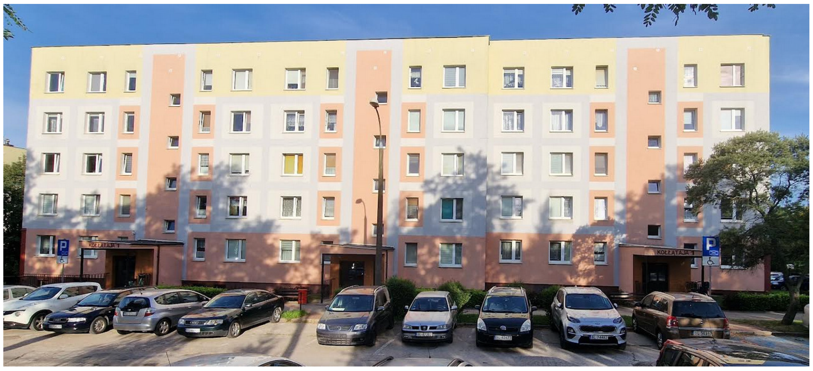
The research conducted on the actual thermal energy consumption includes a total of 22 multi-family residential buildings made with prefabricated technology of the Żerań Brick (CŻ) type and OWT-67N type. The research was carried out from 2002 to 2020. Measurements of thermal energy consumption were carried out using ultrasonic heat meters. During the course of the study, the buildings were subjected to thermo-modernization measures (external walls, ceilings were insulated and windows and doors were replaced), and there was a change in the weather regulation of the central heating system to forecast regulation, which influenced the real change in the measured thermal energy during the measurements.
Table 4 highlights the three periods of thermal energy measurements: before thermal improvement, after thermal improvement (green) and the third period, when the Egain Edge central heating predictive control system was installed in the buildings (yellow), which replaced the weather regulation of the central heating substation (Figure 1).
Only buildings B2, B9 and B10 did not undergo thermal improvement. In these buildings, only a predictive control system for the central heating system was introduced, consisting of continuous predictions of weather conditions, such as outdoor temperature, sunshine, wind and humidity. In all buildings, except building B10, cost allocators for the central heating system were installed. Building B10 had the highest annual average final energy demand index of 126 kWh/(m2·year). The remaining buildings had an average FEH index ranging from 75 kWh/(m2·year) to 102 kWh/(m2·year).
Table 4 shows the index of the annual final energy demand in buildings B1–B22 calculated on the basis of measurements obtained from ultrasonic heat meters according to Relation (1), after taking into account the heated area of each building, which is included in Table 1.
As can be seen in Table 4, in individual years as a result of the work, whether after modernization or after the introduction of the Egain Edge system, the rate of the annual final energy demand during building use varied from 140 kWh/(m2·year) (B10) to 52 kWh/(m2·year) (B22).
Before thermal improvement in buildings B1–B22, but without including building B10, the measured seasonal final energy demand ratio varied from 129 kWh/(m2·year) (B4,B5) to 79 kWh/(m2·year) (B22) in different years.
In buildings B1–B22, which did not undergo thermal improvement, the average energy consumption value (median) was 106 kWh/(m2·year), with the lower limit of the confidence interval being 82 kWh/(m2·year), building B22, and the upper limit being 127 kWh/(m2·year), building B10, as shown in Table 5 and Figure 6.
Figure 7 shows the structure of buildings by the magnitude of the energy demand index for heating before thermal improvement, where weather control is still implemented in the heat source. Among the analyzed buildings, the largest number of buildings had an energy consumption index in the range of 104–112 kWh/(m2·year), and the smallest number of buildings had energy consumption indexes in the range of 120–127 kWh/(m2·year) and 82–88 kWh/(m2·year).
The surveyed buildings were put into use between 1986 and 1994 (Table 1), in accordance with the regulations then in force in Poland. The value of the energy demand index for heating for buildings constructed between 1970 and 1984 was 180–250 kWh/(m2·year). For buildings constructed after 1984, it was 140–180 kWh/(m2·year), and for buildings erected after 1993, it was in the range of 70–140 kWh/(m2·year) [91].
Based on the comparison of the magnitude of the energy demand index for heating before thermal improvement F E H , R in Table 5 and presented graphically in Figure 6, it can be seen that the energy consumption of buildings was not very high. The buildings consumed much less thermal energy than the Technical Conditions that were in force in Poland [91]. Szul and Kokoszka [9] performed a study in 109 buildings made with the same technologies. These buildings had an energy consumption of 164–245 kWh/(m2·year) before thermal improvement, and thus it was nearly 50% higher compared to the energy consumption of the studied group of buildings. Most likely, this was influenced by the introduction in 1995–1997 (except for building B10) of the individual billing of residents by means of cost allocators, the installation of which always greatly affects the reduction in thermal energy consumption in a building. Individual billing, the essence of which is to directly link the number of fees to the registered heat consumption, generally provides an effective financial mechanism to motivate users to rationally manage thermal energy. In the case of the studied group of buildings, this goal was achieved.
Based on the measured thermal energy consumption, this article analyzes various variants of measures to improve energy efficiency. The following were considered: variant 1, involving only the installation of the Egain Edge predictive control system in the buildings (Table 6); variant 2, performing only the thermal improvement of the building body (Table 7); and variant 3, performing thermal improvement together with the installation of the Egain Edge system (Table 8).
The use of an innovative predictive control system, as the first modernization project before the thermal improvement of the building envelope, was performed in the facilities designated as: B1, B2, B3, B5, B7, B9, B10 and B12. After applying the Egain Edge system, the average value (Me) of energy consumption was 90 kWh/(m2·year) and varied from 85.9 kWh/(m2·year), the lower range of the confidence interval, to 92.8 kWh/(m2·year), the upper range. Table 6 shows the average values of energy consumption (median) after the introduction of the predictive regulation of the central heating system, involving continuous predictions of weather conditions in individual buildings.
Another variant that was studied in detail was a variant that included a group of buildings where only thermal improvement was carried out; here, those buildings are marked as: B4, B6, B8, B12–B22. Thermo-modernization was carried out in these buildings, where gable walls, curtain walls, the ceilings, basement windows and exterior entrance doors were insulated, and residents individually replaced windows in their apartments. As part of the thermal improvement, plumbing adjustments of the central heating systems were also carried out. The work was carried out due to available funds in two stages, as shown in Table 1. The completion dates of the work are shown in Table 4.
Table 7 shows energy consumption after carrying out only thermal modernization work on buildings and using weather control at the heat source.
After the thermal modernization work, the average value of energy consumption (median) was 78 kWh/(m2·year) and varied from 75.1 kWh/(m2·year), the lower range of the confidence interval, to 82.2 kWh/(m2·year), the upper range.
The last study of changes in energy consumption in buildings was a variant in which buildings underwent deep thermal improvement and had the Egain Edge weather prediction system installed. A group of buildings was evaluated, labeled as: B1, B3–B8 and B11–B22. Buildings B2, B9 and B10 were not included in the scope because these buildings did not undergo thermal improvement, but they had a predictive control system installed.
Table 8 shows the measured thermal energy consumption of the above-mentioned buildings after thermal improvement and the introduction of the Egain Edge system. The energy consumption is given as an indicator in relation to the heated floor area.
After thermal improvement and the application of the Egain Edge system, the average value of energy consumption was 68 kWh/(m2·year) and varied from 65.6 kWh/(m2·year), the lower limit (of the confidence interval), to 70.4 kWh/(m2·year), the upper limit.
Figure 7 shows in which ranges the heating energy consumption rate changed after the introduction of the three variants discussed above. The chart also illustrates the order in which the projects were carried out in the buildings, where the orange color indicates the initial state before thermal improvement, the green color indicates the installation of the Egain Edge predictive control system and the blue color indicates the implementation of thermal improvement.
As shown in Figure 7, the use of the Egain Edge system resulted in a reduction in heating energy consumption, except for two buildings: B19 and B22.
Based on the thermal energy measured in the buildings with ultrasonic heat meters before and after the application of the Egain Edge system and based on Relation (2), the savings were calculated, which are included in Table 9. According to Table 9, the energy effects obtained after the introduction of predictive regulation in the facilities ranged from 4.5% (building B11) to 25.2% (building B5). The average value of the savings that were achieved was 13.2%. The introduction of predictive regulation made it possible to adjust the parameters of the central heating system to the needs of the residents while maintaining thermal comfort in the premises.
Figure 8 shows the reduction in final energy consumption for central heating after using only the predictive control system (Egain Edge) without thermal improvement of the building.
In contrast, according to Relation (3), the thermal energy savings in buildings where only thermal improvement was performed and weather control was left in the thermal node (without installation of the Egain Edge system) were calculated, which are shown in Table 10. The study included a group of buildings designated as: B4, B6, B8 and B12–B22.
Carrying out thermal improvement in the buildings allowed for saving final energy for heating purposes in the range of 16.45% (building B6) to 41.5% (building B19), and the average value of the achieved savings was 29%.
Table 11 shows the total energy effect taking into account both thermal improvement and the installation of the Egain Edge weather-predictive central heating control system, which was calculated based on Relation (4).
The percentage of savings of the thermal energy consumed for the heating of buildings after deep thermal improvement and after the introduction of forecast regulation in the surveyed buildings ranged from 14.6% (B11) to 45.2% (B15), and the average value of the savings that were obtained was 36.5%. This article also determines the savings that were achieved by replacing weather regulation with forecast regulation of the Egain Edge system in buildings previously subjected to thermal improvement. The savings were determined based on Relation (5), and the results are presented in Table 12. This study included buildings designated as: B4,B6, B8 and B12–B22.
Based on Table 12, except for buildings B19 and B22, replacing weather control with predictive control of the central heating system parameters saved between 2.4% (B4) and 29.5% (B16). The average value of the achieved savings was 8.7%. In two buildings, B19 and B22, the introduction of a system of regulation of the central heating system based on weather prediction (Egain Edge) did not bring the expected results. In these buildings, after the introduction of predictive regulation, energy consumption increased by 5.5% (B19) and 6.9% (B22). This was associated with very low final energy consumption (on average 74–83 kWh/(m2·year) Table 4) already before the introduction of the forecast regulation. In the buildings, the installation of cost allocators resulted in the lowering of indoor temperatures by the residents themselves, at the expense of thermal comfort. In contrast, the predictive control system tried to ensure higher indoor temperatures in the rooms in order to improve the thermal comfort of the residents.
The thermal energy savings after thermal improvement in buildings with a previously installed Egain Edge system were determined from Relation (6) and are shown in Table 13. The study included buildings, designated as: B1, B3, B5, B7 and B11.
The energy efficiency gains from performing this project ranged from 10.6% (B11) to 27.2 (B3), with an average value of 25.3%.

3.2. Economic Analysis

A detailed analysis of the economic viability of the implementation options for projects aimed at improving energy efficiency was carried out, including, in particular, the types of investment costs, the adopted current and forecast prices of thermal energy as well as the expected payback period and the cost of the investment life cycle. In the case of multi-family residential buildings, energy renovations to improve energy efficiency belonged to the group of cost-intensive investments. It was estimated that the average investment costs of energy renovation for 1 m2 of heated usable space per year in residential buildings in EU countries are, on average, 111 EUR/m2 (from 49 EUR/m2 in Latvia to 183 EUR/m2 in Sweden [92]). In Poland, the cost of deep thermal improvement averaged 105 EUR/m2 [18]. According to the data obtained from the housing cooperative to which the buildings subjected to economic evaluation belonged, the average cost of the thermo-modernization works carried out in this group of buildings, subjected to energy efficiency improvements (in 2017–2022), in relation to 1 m2 of heated usable area, was in the range of 90.6 to 124 EUR/m2. The average value for the analyzed group was 109 EUR/m2, which is close to the European average. A reliably performed economic analysis of a particular solution should be based on objective criteria. It is commonly believed that such a criterion is the excess of effects over inputs. Hence, the economic analysis was made on the basis of methods of evaluating physical investments, based on the interest (discount) rate, taking into account the change in the value of money over time. Such a criterion can include life cycle costs (LCC) and the cost of saved energy (CCE). Capital expenditures (Ic) and operating costs (Ce, o) for the different variants were assumed in the form of unit rates related to 1 m2 of heated usable area per year.
Table 14 shows the actual investment and operating costs for individual buildings, as well as the amount of power ordered for heating buildings.
Capital expenditures for the installation of the Egain Edge predictive control system ranged from 0.28 to 1.29 EUR/m2. The average value for the study group was 0.68 EUR/m2. The operating costs associated with the use and maintenance of the Egain system averaged 0.26 EUR/m2. The costs for heating buildings were divided into fixed and variable costs, the size of which was determined by the heat supplier serving the area. The fixed costs depended on the amount of power ordered and ranged from 1.08 (B21) to 1.82 EUR/(m2·year) (B11).
The average value of the fee for ordered power was 1.49 EUR/(m
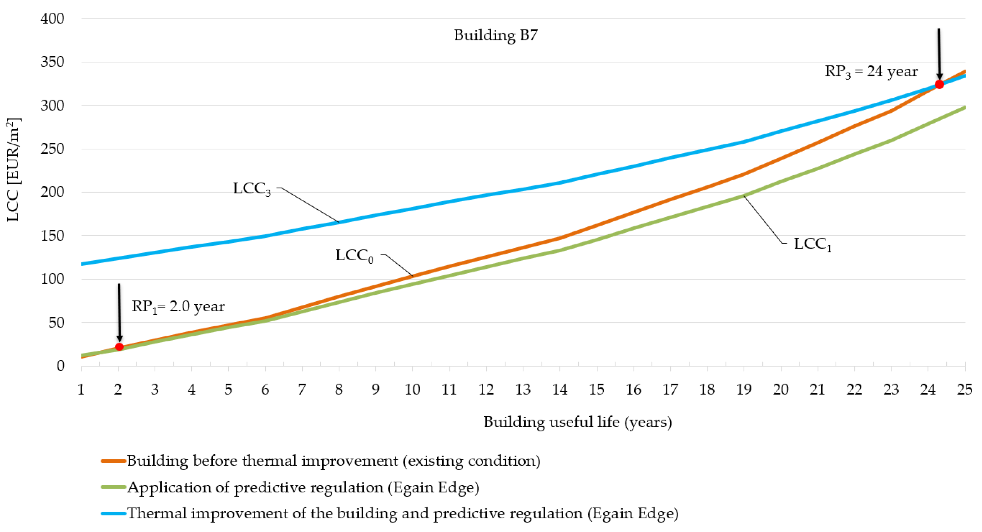
2·year). Variable costs refer to the amount of thermal energy consumed for heating and amount to 0.043 EUR/kWh. The adopted investment and operating expenditures were first used to calculate the life cycle costs for the adopted modernization variants. For the exemplary B7 building, which was characterized by energy consumption before thermal improvement at the level of 107.5 kWh/(m2·year), life cycle cost indicators were calculated before the modernization LCC0 and after the modernization projects LCC1, the application of forecast regulation (Egain Edge), and LCC3, the implementation of the improvement, for the thermal efficiency of building with the use of forecast regulation. The calculations were made from the 1st to the 25th year of using the building, in accordance with the Relation (7), and the results of the calculations are shown in Figure 9.
If the status quo (LCC0 variant) was maintained, the life cycle costs over the assumed 25-year lifetime would be 338.8 EUR per m2 of heated usable area of the building, as shown in Figure 9 and Table 15. The introduction of the Egain Edge system would bring the value of the index down to 297.7 EUR/m2. The thermal improvement of the building (with the Egain Edge system), which resulted in a 40% reduction in energy compared to the baseline due to the high investment costs associated with the thermal improvement (amounting to 109 EUR/m2), resulted in a reduction in the value of the LCC3 index to 334.0 EUR/m2. The calculation of the LCC indexes for each year of assumed operation made it possible to determine the payback period of the investment (RP1 and RP3). The payback periods are illustrated in the graph at the intersection of the LCC0 life cycle cost line with the LCC1 and LCC3 indicator lines. As can be seen in the graph (Figure 9), the expenses incurred for the installation and related maintenance and operating costs are paid back after just two heating seasons. In the case of applying thermal improvement consisting of the implementation of deep thermal modernization, the period of return on investment expenditures at the current energy prices, are extended to 24 years.
The calculations of life cost ratios, according to Relation (7), and the payback time for the other buildings were performed in a similar manner, and the results are shown in Table 15.
Based on an analysis of the results shown in Table 15, it can be seen that the value of the LCC0 life cycle cost index before building retrofit projects ranged from 253.9 (B22) to 368.8 (B8) EUR/m2. The average value was 309 EUR/m2. Buildings with a final energy demand rate for heating higher than 100 kWh/(m2·year) had an LCC0 value of 325 EUR/m2. Buildings with consumption lower than 100 kWh/(m2·year) were characterized by lower index values, which averaged 275 EUR/m2. The introduction of the Egain Edge system allowed for reductions in the value of the LCC1 index to the average value of 276.8 EUR/m2. The level of cost reduction was not significantly influenced by the energy consumption of heating in buildings before the introduction of the weather forecast control system. Depending on the building, the investment returned in the period from 1 to 7 years, most often after 3–4 heating seasons. The performance of thermal improvement did not reduce the value of the LCC2 index, which, in the assumed 25-year service life, is higher than before the improvement, and for buildings subjected to thermal modernization, it amounted to an average of 337 EUR/m2. This state of affairs resulted from high investment costs and relatively small savings (an average of 29%) obtained as a result of the undergoing thermal improvement. The data analysis shows that the least favorable financial effects expressed by the LCC2 indicator were obtained in buildings that were characterized by a relatively low energy consumption before thermo-modernization, oscillating around the value of the final energy demand indicator for heating of 100 kWh/(m2·year) and below this value (buildings B8, B12, B13, B16, B17, B20, B21 and B22). The value of the LCC2 ratios directly translate into the payback period, which, for 12 of the 14 buildings undergoing thermal improvements, exceeds 25 years and can reach 30 to 40 years. The longest payback period for thermal improvement is in buildings with low energy consumption (before thermo-modernization) of 80 to 100 kWh/(m2·year). For example, in building B12, which had a final energy consumption for heating before the thermal improvement of 92 kWh/(m2·year), the investment costs incurred for thermal improvement are recouped only after about 44 years. Similar results can be observed in buildings where thermal improvement was introduced in conjunction with the use of the Egain Edge system. In addition, in this case, it was observed that, as the energy demand became lower, the investment returns became longer (B11, B12 and B22). In the case of Variant 3 (LCC3), in two cases (B19 and B22) the use of Egain Edge negatively affected the values of the indicators, which were higher compared to Variant 2 (LCC2).
Another criterion for evaluating the energy efficiency of the introduced energy-saving solutions was the calculation of the cost of saved energy CCEi. If the value of this indicator was less than or equal to the price paid for energy, there were indications that the investment was profitable. Calculations were made for three retrofit variants, according to Relation (8). The first of these was variant CCE1, the installation of the Egain Edge system, for which the results of the calculations are summarized in Table 16.
Analyzing the results of Table 16, it can be concluded that the installation of the Egain Edge system in buildings not subjected to thermal improvements is a cost-effective investment, as evidenced by the values of indicators for most buildings. The exceptions may be two buildings, B10 and B11, for which the indicators were higher than the price of purchased energy. The high values of these indices were due to the fact that, in the case of these buildings, the achieved thermal energy savings were about 4.5–4.7%. In the remaining buildings, the value of the CCE1 indices fluctuated in the range of 0.013–0.037 EUR/kWh. The average value was 0.026 EUR/kWh and thus was about 50% lower than the cost of purchasing energy.
Other variants for which calculations of the cost of saved energy were performed were thermo-modernization activities consisting of the thermal improvement of CCE2 external partitions. The values of the indicators for this variant are presented in Table 17.
Table 18 shows the results of CCE3 calculations for Variant 3, where comprehensive thermal modernization measures were applied along with the installation of a predictive control system (Egain Edge).
None of the values shown in Table 17 and Table 18 meet the economic efficiency condition: 0 < CCEi < 0.056 EUR/kWh.
The values of the indices for the analyzed Variants 2 and 3, with actual investment, operating costs and achieved savings, ranged for CCE2 from 0.29 to 1.39 EUR/kWh and for CCE3 from 0.22 to 0.88 EUR/kWh. The average value of the CCE2 index exceeded the upper value of the economic efficiency condition by seven times. In the case of Variant 3, the CCE3 index was five times higher than the limit value. Particularly unfavorable indicator values were recorded for buildings B12 (in Variant 2) and B11 (in Variant 3), where energy consumption before thermal improvements was about 90 kWh/(m2·year). Equally unfavorable indicator values were recorded for buildings that had energy consumption below 100 kWh/(m2·year). This clearly shows that this type of investment, which is necessary due to energy policies as well as environmental considerations, should be able to receive financial support in order to be profitable and be undertaken by the investor.

4. Conclusions and Perspectives

On the basis of 19 years of research conducted on a group of 22 residential multi-family buildings located in a temperate continental climate, made with two different technologies based on prefabricated elements (Żerań brick (CŻ) and OWT-67N), in which a predictive control system for the central heating system was installed and deep thermo-modernization was carried out, the following conclusions can be drawn:
In buildings where radiator cost allocators were installed, the measured thermal energy consumption before thermal modernization was much lower than in buildings that were made with similar technologies and that were put into use in 1986–1994. The average value of thermal energy consumption was 106 kWh/(m2·year), with a confidence interval of 104–108 kWh/(m2·year). This was influenced by the introduction of individual billing for residents, where the amount of central heating charges incurred was linked to thermal energy management.
The introduction of a system of predictive control (Egain Edge) of the central heating system based on continuous prediction of weather conditions, even before deep thermo-modernization was carried out, resulted in a reduction in thermal energy by an average of 13.2%, with energy effects varying from 4.5% to 25.2%. The average energy consumption was 90 kWh/(m2·year) and varied from 85.9 kWh/(m2·year) to 92.8 kWh/(m2·year).
The introduction of predictive control made it possible to adjust the parameters of the central heating system to the needs of the residents while maintaining thermal comfort in rooms where, due to excessive and exaggerated conservation of thermal energy, it was not always maintained (B19, B22).
The performance in buildings with cost allocators, with only deep thermo-modernization without installing the Egain Edge system, saved final energy for heating by an average of 29%, with energy effects ranging from 16.45% to 41.5%. The average energy consumption was 78 kWh/(m2·year) and varied in the range of 75.1–82.2 kWh/(m2·year).
The performance of thermal improvements in the buildings, together with the installation of the Egain Edge system in the heat substation, allowed for energy savings of 36.5% on average. Energy savings in the surveyed facilities ranged from 14.6% to 45.2%. The average energy consumption was 68 kWh/(m2·year) and varied from 65.6 kWh/(m2·year) to 70.4 kWh/(m2·year).
In buildings previously subjected to thermal upgrading, where the next stage of modernization work replaced traditional weather control at the district heating substation with predictive control, by installing the Egain Edge system, an average of 8.7% savings was achieved. Energy effects ranged from 2.4% to 29.5%. In two buildings, energy consumption increased by 5.5% (B19) and 6.9% (B22) after the forecast adjustment. This was likely due to very low final energy consumption, averaging 74–83 kWh/(m2·year) before the introduction of the predictive regulation, compared to other buildings.
The average cost of the thermal improvement work that was carried out in this group of buildings averaged 109 EUR/m2, ranging from 90.6 to 124 EUR/m2.
Based on the economic analysis, it can be seen that a large share of the cost of heating buildings is accounted for by fixed costs, which depend on the amount of power ordered and the prices set by the heat supplier. The average value of the fee for ordered power was 1.49 EUR/(m2·year), and the variable fee, which depended on the amount of heat consumed, was 0.043 EUR/kWh. Hence, it is very important to reduce the power ordered from the heat supplier after carrying out thermal upgrading work. Very often, heat suppliers compensate for the lower consumption of heat energy by users by raising the fixed costs for the connection power.
The value of the life cycle cost index translates into the payback period of the investment. The least favorable financial effects expressed by the LCC indicator are obtained in buildings that had relatively low energy consumption before thermo-modernization, with about 100 kWh/(m2·year) and below this value. For such buildings, the payback period is above 25 years.
The installation of the Egain Edge system in non-thermally upgraded buildings is a cost-effective investment. It allows for a reduction in the value of the LCC1 index to an average value of 276.8 EUR/m2. The venture pays for itself in 1 to 7 years, depending on the building, on average after 3–4 years. The average value of the CCE1 index is 0.026 EUR/kWh and is, on average, about 50% lower than the cost of purchasing thermal energy.
The cost ratios of the saved energy CCE3 after deep thermal modernization with the installation of the Egain Edge system in any building did not meet the condition of economic efficiency: 0 < CCEi < 0.056 EUR/kWh.
Actual measurement results from 19 years can be used to test mathematical models using rough set theory to perform simulations of thermal energy consumption in buildings equipped with predictive control systems.
In further research, the authors plan to test the usefulness of the predictive control system in other types of buildings, such as public buildings, e.g., schools, kindergartens and others.

Author Contributions

Conceptualization, J.P.-W. and T.S.; data curation, K.C.; investigation, J.P.-W. and T.S.; methodology, J.P.-W. and T.S.; project administration, J.P.-W. and T.S; supervision, J.P.-W., T.S. and J.K.; writing—original draft preparation, J.P-W., T.S. and K.C.; writing—review and editing, J.P.-W. and T.S. All authors have read and agreed to the published version of the manuscript.

Funding

This work was supported by the Agricultural University of H. Kołłątaja in Krakow and the Białystok University of Technology and was financed by the Ministry of Science and Higher Education of the Republic of Poland (WZ/WBiIS/4/2020).

Institutional Review Board Statement

Not applicable.

Informed Consent Statement

Not applicable.

Data Availability Statement

Not applicable.

Acknowledgments

Meteorological data from the Institute of Meteorology and Water Management—National Research Institute (IMGW-PIB) for the city of Łomża are available courtesy of MPEC Łomża Heating Plant. We would like to thank the Łomża Housing Cooperative for providing data on energy consumption in buildings equipped with the Egain Edge system.

Conflicts of Interest

The authors declare no conflict of interest.

References

  1. United Nations. Act of 20 May 2016 on Energy Efficiency. Journal of Laws 2016, Item 831. Available online: https://isap.sejm.gov.pl/isap.nsf/download.xsp/WDU20160000831/U/D20160831Lj.pdf (accessed on 3 June 2022).
  2. International Energy Agency; United Nations Environment Programme. 2018 Global Status Report: Towards a Zero-Emission, Efficient and Resilient Buildings and Construction Sector. 2018. Available online: https://wedocs.unep.org/20.500.11822/27140 (accessed on 11 June 2022).
  3. BPIE. Europe’s Buildings under the Microscope. A Country-by-Country Review of the Energy Performance of Buildings. 2011. Available online: https://www.bpie.eu/publication/europes-buildings-under-the-microscope (accessed on 11 June 2022).
  4. United Nations. Directive 2010/31/EU of the European Parliament and of the Council of 19 May 2010 on the Energy Performance of Buildings. Available online: https://eur-lex.europa.eu/legal-content/PL/TXT/PDF/?uri=CELEX:32010L0031&from=EL (accessed on 11 June 2022).
  5. United Nations. Directive 2018/844 of the European Parliament and of the Council of 30 May 2018 Amending Directive 2010/31/EU on the Energy Performance of Buildings and Directive 2012/27/EU on Energy Efficiency. Available online: http://data.europa.eu/eli/dir/2018/844/oj (accessed on 30 June 2022).
  6. United Nations. Directive 2018/2002 of the European Parliament and of the Council of 11 December 2018 Amending Directive 2012/27/EU on Energy Efficiency. Available online: http://data.europa.eu/eli/dir/2018/2002/oj (accessed on 30 June 2022).
  7. European Union. European Union Information Papers 2021—Energy Efficiency. Available online: https://www.europarl.europa.eu/ftu/pdf/pl/FTU_2.4.8.pdf (accessed on 30 June 2022).
  8. Lis, P.; Sekret, R. Energy efficiency of buildings-selected problem issues. Energy Mark. 2016, 6, 29–35. Available online: http://yadda.icm.edu.pl/baztech/element/bwmeta1.element.baztech-dcd9364e-6cc9-427e-b150-3fbae739f649?q=bwmeta1.element.baztech-a4741551-e340-47a9-887d-714a9ba80911;4&qt=CHILDREN-STATELESS (accessed on 12 June 2022).
  9. Szul, T.; Kokoszka, S. Application of Rough Set Theory (RST) to Forecast Energy Consumption in Buildings Undergoing Thermal Modernization. Energies 2020, 13, 1309. [Google Scholar] [CrossRef] [Green Version]
  10. Piotrowska-Woroniak, J. The Photovoltaic Installation Application in the Public Utility Building. Ecol. Chem. Eng. S 2020, 24, 517–538. [Google Scholar] [CrossRef] [Green Version]
  11. Szul, T.; Nęcka, K.; Lis, S. Application of the Takagi-Sugeno Fuzzy Modeling to Forecast Energy Efficiency in Real Buildings Undergoing Thermal Improvement. Energies 2021, 14, 1920. [Google Scholar] [CrossRef]
  12. Woroniak, G.; Piotrowska-Woroniak, J. Effects of pollution reduction and energy consumption reduction in small churches in Drohiczyn community. Energy Build. 2014, 72, 51–61. [Google Scholar] [CrossRef]
  13. Broujeny, R.S.; Madani, K.; Chebira, A.; Amarger, V.; Hurtard, L. Data-Driven Living Spaces’ Heating Dynamics Modeling in Smart Buildings using Machine Learning-Based Identification. Sensors 2020, 20, 1071. [Google Scholar] [CrossRef] [PubMed] [Green Version]
  14. Lee, S.; Jung, S.; Lee, J. Prediction Model Based on an Artificial Neural Network for User-Based Building Energy Consumption in South Korea. Energies 2019, 12, 608. [Google Scholar] [CrossRef] [Green Version]
  15. Broujeny, R.S.; Madani, K.; Chebira, A.; Amarger, V.; Hurtard, L. A Heating Controller Designing Based on Living Space Heating Dynamic’s Model Approach in a Smart Building. Energies 2021, 14, 998. [Google Scholar] [CrossRef]
  16. Sun, K.; Hong, T. A framework for quantifying the impact of occupant behavior on energy savings of energy conservation measures. Energy Build. 2017, 146, 383–396. [Google Scholar] [CrossRef] [Green Version]
  17. Brom, P.; Hansen, A.R.; Gram-Hanssen, K.; Meijer, A.; Visscher, H. Variances in residential heating consumption—Importance of building characteristics and occupants analysed by movers and stayers. Appl. Energy 2019, 250, 713–728. [Google Scholar] [CrossRef]
  18. Sadowska, B.; Piotrowska-Woroniak, J.; Woroniak, G.; Sarosiek, W. Energy and Economic Efficiency of the Thermomodernization of an Educational Building and Reduction of Pollutant Emissions—A Case Study. Energies 2022, 15, 2886. [Google Scholar] [CrossRef]
  19. Lu, L.; Cai, W.; Xie, L.; Li, S.; Soh, Y.C. HVAC system optimization—In-building section. Energy Build. 2005, 37, 11–22. [Google Scholar] [CrossRef]
  20. Karimipanah, T. Some Aspects of HVAC Design in Energy Renovation of Buildings. In Urban Transition—Perspectives on Urban Systems and Environments; Wallhagen, P.M., Cehlin, M., Eds.; IntechOpen: London, UK, 2021. [Google Scholar] [CrossRef]
  21. Asim, N.; Badiei, M.; Mohammad, M.; Razali, H.; Rajabi, A.; Haw, L.C.; Ghazali, M.J. Sustainability of Heating, Ventilation and Air-Conditioning (HVAC) Systems in Buildings—An Overview. Int. J. Environ. Res. Public Health 2022, 19, 1016. [Google Scholar] [CrossRef] [PubMed]
  22. Ricci, M.; Sdringola, P.; Tamburrino, S.; Puglisi, G.; Di Donato, E.; Ancona, M.A.; Melino, F. Efficient District Heating in a Decarbonisation Perspective: A Case Study in Italy. Energies 2022, 15, 948. [Google Scholar] [CrossRef]
  23. Weissmann, C.; Hong, T.; Graubner, C.-A. Analysis of heating load diversity in German residential districts and implications for the application in district heating systems. Energy Build. 2017, 139, 302–313. [Google Scholar] [CrossRef] [Green Version]
  24. Wei, Y.; Zhang, X.; Shi, Y.; Xia, L.; Pan, S.; Wu, J.; Han, M.; Zhao, X. A review of data-driven approaches for prediction and classification of building energy consumption. Renew. Sustain. Energy Rev. 2018, 82, 1027–1047. [Google Scholar] [CrossRef]
  25. Zhang, D.; Li, S.; Sun, M.; O’Neill, Z. An Optimal and Learning-Based Demand Response and Home Energy Management System. IEEE Trans. Smart Grid 2016, 7, 1790–1801. [Google Scholar] [CrossRef]
  26. Kanthila, C.; Boodi, A.; Beddiar, K.; Amirat, Y.; Benbouzid, M. Building Occupancy Behavior and Prediction Methods: A Critical Review and Challenging Locks. IEEE Access 2021, 9, 79353–79372. [Google Scholar] [CrossRef]
  27. Boodi, A.; Beddiar, K.; Benamour, M.; Amirat, Y.; Benbouzid, M. Intelligent Systems for Building Energy and Occupant Comfort Optimization: A State of the Art Review and Recommendations. Energies 2018, 11, 2604. [Google Scholar] [CrossRef] [Green Version]
  28. Adegbenro, A.; Short, M.; Angione, C. An Integrated Approach to Adaptive Control and Supervisory Optimisation of HVAC Control Systems for Demand Response Applications. Energies 2021, 14, 2078. [Google Scholar] [CrossRef]
  29. Thieblemont, H.; Haghighat, F.; Ooka, R.; Moreau, A. Predictive control strategies based on weather forecast in buildings with energy storage system: A review of the state-of-the art. Energy Build. 2017, 153, 485–500. [Google Scholar] [CrossRef] [Green Version]
  30. Hou, J.; Li, H.; Nord, N.; Huang, G. Model predictive control under weather forecast uncertainty for HVAC systems in university buildings. Energy Build. 2021, 257, 111793. [Google Scholar] [CrossRef]
  31. Chong, D.; Zhu, N.; Luo, W.; Pan, X. Human thermal risk prediction in indoor hyperthermal environments based on random forest. Sustain. Cities Soc. 2019, 49, 101595. [Google Scholar] [CrossRef]
  32. Hietaharju, P.; Ruusunen, M.; Leiviskä, K. A Dynamic Model for Indoor Temperature Prediction in Buildings. Energies 2018, 11, 1477. [Google Scholar] [CrossRef] [Green Version]
  33. Szul, T.; Tabor, S.; Pancerz, K. Application of the BORUTA Algorithm to Input Data Selection for a Model Based on Rough Set Theory (RST) to Prediction Energy Consumption for Building Heating. Energies 2021, 14, 2779. [Google Scholar] [CrossRef]
  34. Serale, G.; Fiorentini, M.; Capozzoli, A.; Bernardini, D.; Bemporad, A. Model Predictive Control (MPC) for Enhancing Building and HVAC System Energy Efficiency: Problem Formulation, Applications and Opportunities. Energies 2018, 11, 631. [Google Scholar] [CrossRef] [Green Version]
  35. Yang, S.; Wan, M.P.; Chen, W.; Ng, B.F.; Dubey, S. Experiment study of machine-learning-based approximate model predictive control for energy-efficient building control. Appl. Energy 2021, 288, 116648. [Google Scholar] [CrossRef]
  36. Zhang, J.; Wu, Y.; Feng, W.; Wang, J. Spatially Attentive Visual Tracking Using Multi-Model Adaptive Response Fusion. IEEE Access 2019, 7, 83873–83887. [Google Scholar] [CrossRef]
  37. Wang, L.; Dai, L.; Bian, H.; Ma, Y.; Zhang, J. Concrete cracking prediction under combined prestress and strand corrosion. Struct. Infrastruct. Eng. 2019, 15, 285–295. [Google Scholar] [CrossRef]
  38. Xia, Z.; Fang, Z.; Zou, F.; Wang, J.; Sangaiah, A.K. Research on Defensive Strategy of Real-Time Price Attack Based on Multiperson Zero-Determinant. Secur. Commun. Netw. 2019, 2019, 1–13. [Google Scholar] [CrossRef]
  39. Zhang, J.; Wang, W.; Lu, C.; Wang, J.; Sangaiah, A.K. Lightweight deep network for traffic sign classification. Ann. Telecommun. 2019, 75, 369–379. [Google Scholar] [CrossRef]
  40. Chen, Z.; Quan, W.; Wen, M.; Fang, J.; Yu, J.; Zhang, C.; Luo, L. Deep Learning Research and Development Platform: Characterizing and Scheduling with QoS Guarantees on GPU Clusters. IEEE Trans. Parallel Distrib. Syst. 2020, 31, 34–50. [Google Scholar] [CrossRef]
  41. Yu, L.; Xie, D.; Huang, C.; Jiang, T.; Zou, Y. Energy Optimization of HVAC Systems in Commercial Buildings Considering Indoor Air Quality Management. IEEE Trans. Smart Grid 2018, 10, 5103–5113. [Google Scholar] [CrossRef]
  42. Tushar, W.; Wijerathne, N.; Li, W.-T.; Yuen, C.; Poor, H.V.; Saha, T.K.; Wood, K.L. Internet of Things for Green Building Management: Disruptive Innovations Through Low-Cost Sensor Technology and Artificial Intelligence. IEEE Signal Process. Mag. 2018, 35, 100–110. [Google Scholar] [CrossRef]
  43. Dhar, N.K.; Verma, N.K.; Behera, L. Adaptive Critic-Based Event-Triggered Control for HVAC System. IEEE Trans. Ind. Inform. 2018, 14, 178–188. [Google Scholar] [CrossRef]
  44. Patyn, C.; Deconinck, G. Dynamic mode decomposition for nonintrusive and robust model predictive control of residential heating systems. Energy Build. 2022, 254, 111450. [Google Scholar] [CrossRef]
  45. Li, H.; Yan, W.; Shi, Y. Triggering and Control Codesign in Self-Triggered Model Predictive Control of Constrained Systems: With Guaranteed Performance. IEEE Trans. Autom. Control 2018, 63, 4008–4015. [Google Scholar] [CrossRef]
  46. Homod, R.Z. Analysis and optimization of HVAC control systems based on energy and performance considerations for smart buildings. Renew. Energy 2018, 126, 49–64. [Google Scholar] [CrossRef]
  47. Szul, T. Application of a Thermal Performance-Based Model to Prediction Energy Consumption for Heating of Single-Family Residential Buildings. Energies 2022, 15, 362. [Google Scholar] [CrossRef]
  48. Wang, Y.; Bai, Y.; Yang, L.; Li, H. Short time air temperature prediction using pattern approximate matching. Energy Build. 2021, 244, 111036. [Google Scholar] [CrossRef]
  49. Demirezen, G.; Fung, A.S. Application of artificial neural network in the prediction of ambient temperature for a cloud-based smart dual fuel switching system. Energy Procedia 2019, 158, 3070–3075. [Google Scholar] [CrossRef]
  50. Zhang, X.; Tan, S.C.; Li, G. Development of an ambient air temperature prediction model. Energy Build. 2014, 73, 166–170. [Google Scholar] [CrossRef]
  51. Jeong, S.; Park, I.; Kim, H.; Song, C.; Kim, H. Temperature Prediction Based on Bidirectional Long Short-Term Memory and Convolutional Neural Network Combining Observed and Numerical Forecast Data. Sensors 2021, 21, 941. [Google Scholar] [CrossRef] [PubMed]
  52. Park, I.; Kim, H.S.; Lee, J.; Kim, J.H.; Song, C.H.; Kim, H.K. Temperature Prediction Using the Missing Data Refinement Model Based on a Long Short-Term Memory Neural Network. Atmosphere 2019, 10, 718. [Google Scholar] [CrossRef] [Green Version]
  53. Ahn, J.; Cho, S. Development of an intelligent building controller to mitigate indoor thermal dissatisfaction and peak energy demands in a district heating system. Build. Environ. 2017, 124, 57–68. [Google Scholar] [CrossRef]
  54. Lee, C.; Jung, D.E.; Lee, D.; Kim, K.H.; Do, S.L. Prediction Performance Analysis of Artificial Neural Network Model by Input Variable Combination for Residential Heating Loads. Energies 2021, 14, 756. [Google Scholar] [CrossRef]
  55. Papantoniou, S.; Kolokotsa, D.-D. Prediction of outdoor air temperature using neural networks: Application in 4 European cities. Energy Build. 2016, 114, 72–79. [Google Scholar] [CrossRef]
  56. Reich, M.; Gottschald, J.; Riegebauer, P.; Adam, M. Predictive Control of District Heating System Using Multi-Stage Nonlinear Approximation with Selective Memory. Energies 2020, 13, 6714. [Google Scholar] [CrossRef]
  57. Mugnini, A.; Coccia, G.; Polonara, F.; Arteconi, A. Performance Assessment of Data-Driven and Physical-Based Models to Predict Building Energy Demand in Model Predictive Controls. Energies 2020, 13, 3125. [Google Scholar] [CrossRef]
  58. Kathirgamanathan, A.; De Rosa, M.; Mangina, E.; Finn, D.P. Data-driven predictive control for unlocking building energy flexibility: A review. Renew. Sustain. Energy Rev. 2021, 135, 110120. [Google Scholar] [CrossRef]
  59. Kasper, T. The Energy Efficiency Potential of Intelligent Heating Control Approaches in the Residential Sector; Eidgenössische Technische Hochschule Zürich: Zurich, Switzerland, 2013; Available online: https://sustec.ethz.ch/content/dam/ethz/special-interest/mtec/sustainability-and-technology/PDFs/130420%20Master%20thesis%20on%20intelligent%20heating%20control%20approaches%20-%20Thomas%20Kasper_final.pdf (accessed on 30 June 2022).
  60. Persson, J.; Vogel, D. Utnyttjande av Byggnaders Värmetröghet. Utvärdering av Kommersiella Systemlösningar; Lunds Universitet: Lund, Sweden, 2011; ISRN LUTVDG/TVIT—11/5030—SE(68); Available online: http://lup.lub.lu.se/luur/download?func=downloadFile&recordOId=3161459&fileOId=3161460 (accessed on 30 June 2022).
  61. Herrlin, E. Alternativa Reglermetoder för en Energieffektiv Byggnad; KTH Skolan för Kemi Och Hälsa: Stockholm, Sweden, 2017; Available online: http://kth.diva-portal.org/smash/get/diva2:1143765/FULLTEXT02.pdf (accessed on 5 October 2020).
  62. Enreduce Energy Control AB. Knowledge, Experience and A Unique Energy Management System. Available online: https://www.enreduce.se/om-oss/ (accessed on 30 May 2022).
  63. Oldewurtel, F.; Parisio, A.; Jones, C.N.; Gyalistras, D.; Gwerder, M.; Stauch, V.; Lehmann, B.; Morari, M. Use of model predictive control and weather forecasts for energy efficient building climate control. Energy Build. 2012, 45, 15–27. [Google Scholar] [CrossRef] [Green Version]
  64. Hilding, O.; Nilsson, S. Analysis and Development of Control Strategies for a District Heating Central; Chalmers University of Technology: Gothenburg, Sweden, 2009; Available online: http://publications.lib.chalmers.se/records/fulltext/99408.pdf (accessed on 18 October 2020).
  65. Cox, R.A.; Drews, M.; Rode, C.; Nielsen, S.B. Simple future weather files for estimating heating and cooling demand. Build. Environ. 2015, 83, 104–114. [Google Scholar] [CrossRef] [Green Version]
  66. Bacher, P.; Madsen, H.; Nielsen, H.A.; Perers, B. Short-term heat load forecasting for single family houses. Energy Build. 2013, 65, 101–112. [Google Scholar] [CrossRef] [Green Version]
  67. Bröms, G.; Isfält, E. Effekt—och Energibesparing Genom Förenklad Styrning och Drift av Installationsystem i Byggnader; Institutionen förinstallationsteknik: Sztokholm, Sweden, 1992; ISSN 0284-141X. Available online: https://www.kabona.com/wp-content/uploads/2015/12/Sammanfattning_teoretisk_bakgrund_Ecopilot.pdf (accessed on 10 June 2022).
  68. Egain Edge. Available online: https://www.egain.io/pl/nasz-platforma/technologia/#sztuczna-inteligencja (accessed on 21 June 2022).
  69. Piotrowska-Woroniak, J.; Cieśliński, K.; Woroniak, G.; Bielskus, J. The Impact of Thermo-Modernization and Forecast Regulation on the Reduction of Thermal Energy Consumption and Reduction of Pollutant Emissions into the Atmosphere on the Example of Prefabricated Buildings. Energies 2022, 15, 2758. [Google Scholar] [CrossRef]
  70. Cieśliński, K.; Tabor, S.; Szul, T. Evaluation of Energy Efficiency in Thermally Improved Residential Buildings, with a Weather Controlled Central Heating System. A Case Study in Poland. Appl. Sci. 2020, 10, 8430. [Google Scholar] [CrossRef]
  71. Huang, H.; Chen, L.; Hu, E. A neural network-based multi-zone modelling approach for predictive control system design in commercial buildings. Energy Build. 2015, 97, 86–97. [Google Scholar] [CrossRef]
  72. Arabali, A.; Ghofrani, M.; Etezadi-Amoli, M.; Fadali, M.S.; Baghzouz, Y. Genetic-Algorithm-Based Optimization Approach for Energy Management. IEEE Trans. Power Deliv. 2013, 28, 162–170. [Google Scholar] [CrossRef]
  73. Fang, J.; Ma, R.; Deng, Y. Identification of the optimal control strategies for the energy-efficient ventilation under the model predictive control. Sustain. Cities Soc. 2019, 53, 101908. [Google Scholar] [CrossRef]
  74. Moon, J.W. Performance of ANN-based predictive and adaptive thermal-control methods for disturbances in and around residential buildings. Build. Environ. 2012, 48, 15–26. [Google Scholar] [CrossRef]
  75. Hietaharju, P.; Ruusunen, M.; Leiviskä, K. Enabling Demand Side Management: Heat Demand Forecasting at City Level. Materials 2019, 12, 202. [Google Scholar] [CrossRef] [PubMed]
  76. Wang, J.; Gao, Y.; Liu, W.; Wu, W.B.; Lim, S. An Asynchronous Clustering and Mobile Data Gathering Schema Based on Timer Mechanism in Wireless Sensor Networks. Comput. Mater. Contin. 2019, 58, 711–725. [Google Scholar] [CrossRef] [Green Version]
  77. Al-Shammari, E.T.; Keivani, A.; Shamshirband, S.; Mostafaeipour, A.; Yee, P.L.; Petković, D.; Chintalapati, S. Prediction of heat load in district heating systems by Support Vector Machine with Firefly searching algorithm. Energy 2016, 95, 266–273. [Google Scholar] [CrossRef]
  78. He, S.; Xie, K.; Xie, K.; Xu, C.; Wang, J. Interference-Aware Multisource Transmission in Multiradio and Multichannel Wireless Network. IEEE Syst. J. 2019, 13, 2507–2518. [Google Scholar] [CrossRef]
  79. Wang, J.; Gao, Y.; Liu, W.; Sangaiah, A.K.; Kim, H.-J. An intelligent data gathering schema with data fusion supported for mobile sink in wireless sensor networks. Int. J. Distrib. Sens. Netw. 2019, 15, 1550147719839581. [Google Scholar] [CrossRef] [Green Version]
  80. Sajjadi, S.; Shamshirband, S.; Alizamir, M.; Yee, P.L.; Mansor, Z.; Manaf, A.A.; Altameem, T.A.; Mostafaeipour, A. Extreme learning machine for prediction of heat load in district heating systems. Energy Build. 2016, 122, 222–227. [Google Scholar] [CrossRef]
  81. Adamczyk, J.; Dylewski, R. Ecological and Economic Benefits of the “Medium” Level of the Building Thermo-Modernization: A Case Study in Poland. Energies 2020, 13, 4509. [Google Scholar] [CrossRef]
  82. Dębowski, J. The Whole Truth about Large-Plate Buildings; Building Review, Krakow, Poland 2012, 83/9; BazTech, 2012; pp. 28–35. Available online: https://yadda.icm.edu.pl/baztech/element/bwmeta1.element.baztech-article-BTB6-0005-0012?q=bwmeta1.element.baztech-volume-0033-2038-przeglad_budowlany-2012-r__83_nr_9;3&qt=CHILDREN-STATELESS (accessed on 18 June 2022).
  83. Hummel, M.; Büchele, R.; Müller, A.; Aichinger, E.; Steinbach, J.; Kranzl, L.; Toleikyte, A.; Forthuber, S. The costs and potentials for heat savings in buildings: Refurbishment costs and heat saving cost curves for 6 countries in Europe. Energy Build. 2021, 231, 110454. [Google Scholar] [CrossRef]
  84. Liu, L.; Moshfegh, B.; Akander, J.; Cehlin, M. Comprehensive investigation on energy retrofits in eleven multi-family buildings in Sweden. Energy Build. 2014, 84, 704–715. [Google Scholar] [CrossRef]
  85. Chen, X.; Qu, K.; Calautit, J.; Ekambaram, A.; Lu, W.; Fox, C.; Gan, G.; Riffat, S. Multi-criteria assessment approach for a residential building retrofit in Norway. Energy Build. 2020, 215, 109668. [Google Scholar] [CrossRef]
  86. Mauro, G.M.; Hamdy, M.; Vanoli, G.P.; Bianco, N.; Hensen, J.L. A new methodology for investigating the cost-optimality of energy retrofitting a building category. Energy Build. 2015, 107, 456–478. [Google Scholar] [CrossRef]
  87. Institute of Meteorology and Water Management. Data from the Institute of Meteorology and Water Management. Available online: https://danepubliczne.imgw (accessed on 1 July 2022). (In Polish).
  88. Polish Committee for Standardization. PN-EN ISO 6946:2017-10; European Standard: Building Components and Building Elements—Thermal Resistance and Heat Transfer Coefficient. 2017. Available online: https://sklep.pkn.pl/pn-en-iso-6946-2017-10p.html (accessed on 30 June 2022).
  89. Polish Committee for Standardization. PN-EN ISO 12831-1:2017-08; European Standard: Heating Systems in Buildings. CEN, 2007. Available online: https://sklep.pkn.pl/pn-en-12831-3-2017-08e.html (accessed on 30 June 2022).
  90. Peel, M.C.; Finlayson, B.L.; McMahon, T.A. Updated world map of the Köppen-Geiger climate classification. Hydrol. Earth Syst. Sci. 2007, 11, 1633–1644. [Google Scholar] [CrossRef]
  91. Minister of Infrastructure and Construction. Regulation of the Minister of Infrastructure and Construction on Technical Conditions to Be Met by Buildings and Their Location [Journal of Laws June 7, 2019, item 1065]. Available online: https://isap.sejm.gov.pl/isap.nsf/download.xsp/WDU20190001065/O/D20191065.pdf (accessed on 6 July 2022). (In Polish)
  92. European Commission. Comprehensive Study of Building Energy Renovation Activities and the Uptake of Nearly Zero-Energy Buildings in the EU; Final Report; European Union: Brussels, Belgium, 2019; Available online: https://ec.europa.eu/energy/sites/ener/files/documents/1.final_report.pdf (accessed on 18 June 2022).
Figure 1. View of a typical building (B19) accepted for the study, made with OWT -67N large-panel prefabricated technology, 5-story, 3-cage [photo taken by authors].
Energies 15 07279 g001
Figure 2. View of a typical building (B3) adopted for the study, made with large-block prefabricated CŻ technology, 3-story, 2-cage [photo taken by authors].
Energies 15 07279 g002
Figure 3. Compilation and comparison of elements included in heating regulation systems [own study].
Energies 15 07279 g003
Figure 4. Egain Hub weather forecast receiver (a) mounted on the outside wall of the building and the signal transmitter (b) mounted on the heating substation [photo taken by authors].
Energies 15 07279 g004
Figure 5. Number of heating season degree days determined for 2002–2020 based on temperature data of MPEC Łomża Heat Plant and typical heating season (1991–2020) [87].
Energies 15 07279 g005
Figure 6. Structure of buildings by size of heating energy demand index before thermal improvement F E H , R [kWh/(m2·year)].
Energies 15 07279 g006
Figure 7. Change in energy consumption for heating purposes after the introduction of the individual variants.
Energies 15 07279 g007
Figure 8. Reduction in energy consumption for central heating after using predictive control system (Egain Edge) without thermal improvement of the building.
Energies 15 07279 g008
Figure 9. Life cycle costs LCC0, LCC1 and LCC3 using building B7 as an example.
Energies 15 07279 g009
Table 1. Basic technical parameters of the surveyed buildings.
ObjectBuildings B1–B12 Prefabricated Technology Type CŻ
Buildings B13–B22 Prefabricated Technology Type OWT-67N
Year of the Construction of the BuildingBuilding AreaHeated Volume of the Building [m3]A/VNumber of StaircasesYear of Thermal Modernization
Usable AF [m2]Housing [m2]Gable WallsLongitudinal Walls
B119921031656.153950.39220162016
B219921029656.153950.382- *- *
B319921017619.955417.70.37220172017
B4199214899537935.80.38320132013
B5199116881115.88677.40.36320192019
B619911199774.66251.10.38220102010
B7199436032235.218,3760.33620142014
B8199446702409.523,9550.34820102010
B9199543172499.125,1780.317- *- *
B10199623971389.0611,9880.334- *- *
B11199318661237.7596400.34320192019
B12199328961827.7514,7480.30420092009
B1319832292165791970.38420032007
B141984229216579232.60.37420032007
B15198418681292.67558.90.38320032007
B16198424081575.69877.80.38420022007
B17198324231608.29983.60.38420012005
B181983242616859991.80.38420012005
B19198819931918.68459.60.35320012011
B2019882413168610,4040.38420022011
B211986242617,589.710,295.70.38420032009
B2219862665196111,151.20.38420032009
*—buildings that have not been thermo-modernized.
Table 2. Heat transfer coefficients U of building partitions after thermal improvement.
Type of PartitionHeat Transfer Coefficients U [W/(m2·K)]
after Thermal Improvement
Prefabricated Technology
Large-Block CŻLarge-Plate OWT-67N
gable walls0.190.26
longitudinal walls0.190.24
ventilated flat roofs0.180.18
entrance doors1.501.50
windows in staircases1.101.10
windows in basements1.101.30
Table 3. Energy performance of surveyed buildings before and after thermal improvements [89].
Buildings Under StudyCalculated Thermal Power of the Heating System [MW]
Before Thermal ImprovementAfter Thermal Improvement
B10.06000.0570
B20.0584- *
B30.06000.0600
B40.09000.0810
B50.10030.0990
B60.07300.0721
B70.20700.1842
B80.31100.2700
B90.2425- *
B100.1250- *
B110.11800.1049
B120.15990.1396
B130.28480.1081
B140.24800.1133
B150.23050.1161
B160.30290.0937
B170.31230.1180
B180.28950.1187
B190.21760.0980
B200.27650.1243
B210.25260.0919
B220.25810.1280
*—non-insulated buildings.
Table 4. Index of annual final energy demand FEH in the studied facilities B1–B22 from 2002 to 2020 [kWh/(m2·year)].
YearHeating Final Energy Index FEH [kWh/(m2·year)]
B1B2B3B4B5B6B7B8B9B10B11B12B13B14B15B16B17B18B19B20B21B22
20021061071071151151151081081111219393110124114117104118988611595
2003113113113129129129114119120127979710113012111910712410194123101
2004109109109122122122111111117137939310511511511198114889610787
200598979811311311310211096124868610310610299859387929681
200610810810811111011110410873127878710710911699717695909281
20071051051051161161161071008213289899910010795758198979379
2008113113113120120120112111951409292808497908081941029882
2009106106107115115115107110103132838380789290758286998275
20101061061061161161161111041021238989787478887285871006864
2011969596979797928091117848469737083708077866561
2012103103103100100100958287127817468787276687455636454
2013108108108979797918292121907671757678727355627048
2014101102103858381828490120847364686572706855626452
2015898491788067657481118816561676862636253545552
2016839496828673687889130856969736762666759596059
2017739692849275688290138876871787169677160616364
2018679273848873687988122836974776562667757606261
2019709370867972637986118797171736260647059626164
2020698564796370688181110736469656058626356616063
Average value961019810210198919493126868082878584768275787970
Designations: green—building energy consumption one year after thermal improvement; yellow—installation of weather control system Egain Edge.
Table 5. Energy consumption in buildings B1–B22 before thermal improvement; weather control is implemented in the heat source F E H , R in [kWh/m2·year].
BuildingEnergy Consumption Before Thermal Improvement
(Weather Control System) FEH,R [kWh/(m2·year)]
Median (Me)Confidence Interval
Lower LimitUpper Limit
B1106104.2107.8
B2106104108
B3107105.3108.7
B4115111.5118.5
B5115111.5118.5
B6116111.8120.2
B7107.5105110
B8110104.4115.6
B995.590.4100.6
B10127123.3130.7
B118987.290.8
B129290.293.8
B13104102106
B14112106.2117.8
B15114.5111118
B1610599.7110.3
B1710194.9107.1
B18116107.5124.5
B199491.696.4
B209693.998.1
B219892.4103.6
B22827886
Average Value106104.1108.4
Table 6. Annual heating energy consumption index after introduction of Egain Edge system F E H , E (building in existing condition and before thermal improvement) in [kWh/(m2·year)].
Unit Energy Consumption after the Introduction of
the Weather Forecasting System FEH,R [kWh/(m2·year)]
BuildingB1B2B3B5B7B9B10B11Average Value
Median (Me)8693928691881218590
Confidence IntervalLower Limit82.390.485.682.986.186.1117.683.485.9
Upper Limit89.795.698.489.195.989.9124.486.692.8
Table 7. Index of annual energy consumption after thermal improvement of buildings, but with the use of weather control in the heat source F E H , T M [kWh/(m2·year)].
BuildingUnit Energy Consumption after Thermal Improvement
(Weather Control), FEH,TM [kWh/(m2·year)]
Median (Me)Confidence Interval
Lower LimitUpper Limit
B48585.085.0
B69791.6102.4
B88281.182.9
B128480.187.9
B137874.681.4
B147875.680.4
B157871.284.8
B168884.691.4
B177270.373.7
B188179.083.0
B195548.161.9
B206355.670.4
B216763.570.5
B225853.063.0
Average Value7875.182.2
Table 8. Index of annual energy consumption in buildings after thermal improvement and introduction of Egain Edge system F E H , T M [kWh/(m2·year)].
BuildingUnit Energy Consumption after Introducing Egain Edge System
and Performing Thermal Improvement FEH,TM [kWh/(m2·year)]
Median (Me)Confidence Interval
Lower LimitUpper Limit
B17068.471.6
B36763.370.7
B48381.384.7
B5636363
B67371.674.4
B76866.969.1
B87977.580.5
B117672.379.7
B126967.270.8
B137068.171.9
B147370.975.1
B156663.768.3
B166258.965.1
B176664.767.3
B186865.670.4
B195857.158.9
B206160.661.4
B216160.361.7
B226261.362.7
Average Value6865.670.4
Table 9. Energy savings after using Egain Edge predictive control system in buildings before thermal improvement, ES1 (%), [%].
Installation of a Predictive Control System Prior to Thermal Improvement ES1 (%), [%]
BuildingB1B2B3B5B7B9B10B11Average Value
Median (Me)18.912.314.025.215.37.94.74.513.2
Table 10. Energy savings after thermal improvement only (weather control) ES2 (%), %.
Building Thermal Improvement (Weather Control) ES2 (%), [%]
BuildingB4B6B8B12B13B14B15B16B17B18B19B20B21B22Average Value
Median (Me)26.116.425.58.725.030.431.916.228.730.241.534.431.629.329.0
Table 11. Energy savings after thermal improvement and introduction of Egain Edge system ES3 (%), [%].
Building Thermal Improvement and the Installation of Predictive Control ES3 (%), [%]
BuildingB1B3B4B5B6B7B8B11B12B13Average Value B1–B22
Median (Me)34.037.427.845.237.136.728.214.625.032.736.5
BuildingB14B15B16B17B18B19B20B21B22
Median (Me)34.842.441.034.741.438.336.537.824.4
Table 12. Energy savings as a result of replacing weather control with Egain Edge predictive control (after thermal improvement) ES4 (%), [%].
Replacing Weather Regulation with Predictive Regulation ES4 (%), [%]
BuildingB4B6B8B12B13B14B15B16B17B18B19B20B21B22Average Value
Median (Me)2.424.73.717.910.36.415.429.58.316−5.53.29−6.98.7
Table 13. Energy savings after thermal improvement in buildings equipped with Egain Edge systems, ES5 (%), [%].
Thermal Improvement of a Building Equipped with a Predictive Control System, ES5 (%), [%]
BuildingB1B3B5B7B11Average value
Median (Me)18.627.226.725.310.625.3
Table 14. A statement of the adopted costs for conducting the economic analysis.
BuildingPower Ordered [MW]Egain Edge SystemHeating Fee
Installation [EUR/m2]Operation [EUR/m2]Costs
Fixed [EUR/m2·year]Variable [EUR/kWh]
B10.05701.280.281.580.043
B20.05841.280.281.620.043
B30.06001.290.281.680.043
B40.08100.880.271.550.043
B50.09900.780.261.670.043
B60.07211.100.271.720.043
B70.18420.370.251.460.043
B80.27000.280.251.650.043
B90.25140.300.251.660.043
B100.12500.550.261.490.043
B110.10490.800.271.820.043
B120.13960.370.251.120.043
B130.10810.570.261.350.043
B140.11330.570.261.410.043
B150.11610.700.261.780.043
B160.09370.550.261.110.043
B170.11800.540.261.390.043
B180.11870.540.261.400.043
B190.09800.660.261.400.043
B200.12430.540.261.470.043
B210.09190.540.261.080.043
B220.12800.490.261.370.043
Table 15. Life cycle cost index before retrofit LCC0 [EUR/m2] and after retrofit projects LCC1–LCC3 [EUR/m2] and payback time on investment RP1–RP3 [years].
BuildingLife Cycle Cost Index [EUR/m2]Payback Time on Investment [years]
LCC0 LCC1LCC2LCC3RP1RP2RP3
Variant 0Variant 1Variant 2Variant 3Variant 1Variant 2Variant 3
B1300.3250.2-315.73-26
B2300.3268.8- -4--
B3302.7266.1-308.64-27
B4316.0-349.0345.0-3028
B5319.36247.1-298.21-23
B6313.0-374.2316.4-3526
B7338.8297.7-334.02-24
B8368.8-395.6391.2-2726
B9335.3293.0--3--
B10355.5340.9--6--
B11259.8250.7- 331.07-39
B12279.1 -362.1324.7 -4434
B13300.5- 355.2315.6- 3227
B14323.6 -338.2326.3 -2625
B15329.9- 338.2308.6- 2623
B16294.2 -357.4292.5 -3624
B17313.6- 326.0311.4- 2725
B18354.4 -348.7316.5 -2421
B19281.2- 277.2285.5- 2426
B20289.2- 303.3298.9- 2726
B21288.3- 304.5290.1- 2826
B22253.9- 290.7301.5- 3134
Description: Variant 0 is the period before thermal improvement; Variant 1 is the installation of the Egain Edge system; Variant 2 is the execution of thermal improvement; and Variant 3 is the execution of thermal improvement and the installation of the Egain Edge system.
Table 16. Value of cost index of saved thermal energy after installation of Egain Edge system in buildings before thermal improvement CCE1 [EUR/kWh].
Cost Index of Saved Heat Energy CCE1, [EUR/kWh]
Installation of Egain Edge System (Variant 1)
BuildingB1B2B3B5B7B9B10B11
CCE10.0240.0360.0310.0130.0180.0370.0570.097
Table 17. Value of cost index of saved energy for heating after thermal improvement only (weather control) CCE2, [EUR/kWh].
Cost Index of Saved Heat Energy CCE2, [EUR/kWh]
Implementation of Thermal Improvement (Variant 2)
BuildingB4B6B8B12B13B14B15B16B17B18B19B20B21B22
CCE20.370.590.401.390.430.330.300.650.380.320.290.340.360.46
Table 18. Value of cost index of saved energy for heating after thermal improvement with installation of Egain Edge predictive control system CCE3, [EUR/kWh].
Cost Index of Saved Heat Energy CCE3, [EUR/kWh]
Execution of Thermal Improvement and the Installation of the Egain Edge System (Variant 3)
BuildingB1B3B4B5B6B7B8B11B12B13
CCE30.320.290.360.220.270.290.370.880.500.34
Building B14B15B16B17B18B19B20B21B22
CCE30.290.230.270.330.240.320.330.310.57
Publisher’s Note: MDPI stays neutral with regard to jurisdictional claims in published maps and institutional affiliations.

