Estimation of Seismic Wave Attenuation from 3D Seismic Data: A Case Study of OBC Data Acquired in an Offshore Oilfield

Abstract

Previous studies performed in Abu Dhabi oilfields, United Arab Emirates, revealed the direct link of seismic wave attenuation to petrophysical properties of rocks. However, all those studies were based on zero offset VSP data, which limits the attenuation estimation at one location only. This is due to the difficulty of estimating attenuation from 3D seismic data, especially in carbonate rocks. To overcome this difficulty, we developed a workflow based on the centroid frequency shift method and Gabor transform which is optimized by using VSP data. The workflow was applied on 3D Ocean Bottom Cable seismic data. Distinct attenuation anomalies were observed in highly heterogeneous and saturated zones, such as the reservoirs and aquifers. Scattering shows significant contribution in attenuation anomalies, which is unusual in sandstones. This is due to the complex texture and heterogeneous nature of carbonate rocks. Furthermore, attenuation mechanisms such as frictional relative movement between fluids and solid grains, are most likely other important causes of attenuation anomalies. The slight lateral variation of attenuation reflects the lateral homogeneous stratigraphy of the oilfield. The results demonstrate the potential of seismic wave attenuation for delineating heterogeneous zones with high fluid content, which can substantially help for enhancing oil recovery.

1. Introduction

Enhanced oil recovery (EOR) aims to improve oil and gas production by facilitating the flow of fluids. The three major EOR techniques are chemical flooding [1], miscible displacement [2] and thermal recovery [2]. The optimal application of each technique depends on petrophysical properties of reservoirs such as permeability, water saturations, porosity and fluid properties. Fracture network, control the hydraulic and many reservoir petrophysical properties. Therefore, receiving fractures properties is crucial for applying EOR techniques. Conventional methods used for investigating naturally fractured reservoirs are generally based on petro-physical well-logs, such as sonic, gamma ray, and resistivity logs or on core description. However, such data are obtained in the vicinity of the well location and at small scale. At large scale, fracture properties are obtained from surface seismic data by applying stiffness anisotropy and geometry-based methods. Chichinina and Martyushev [3] compared Thomson’s anisotropy parameters in dry and saturated cracked rocks. They found out that in dry rock $\gamma$ is much smaller than $\epsilon$, while $\delta$ is larger than $\epsilon$ and becomes negative when the rock is fully saturated. By looking at the dominant direction of the extracted maximum curvature, Ali, et al. [4] successfully defined the dominant orientation of fractures in a reservoir of an offshore Abu Dhabi oilfield, and found that it is parallel to the NNE-SSW and NE-SW directions. However, such methods are sensitive to any geological feature causing seismic anisotropy other than fractures, such as lithological alignment.

Theoretical [5], experimental [6], and field studies [7] have demonstrated the potential and superiority of seismic wave attenuation for studying fractured rocks. Previous study in one of Abu Dhabi oilfields, showed the advantage of integrating seismic attenuation to characterize fractured carbonate reservoirs [7]. Bouchaala, et al. [8] was able to separate between open and cemented fractures by using seismic wave attenuation anisotropy. Yang, et al. [9] simultaneously took into account the effect of anisotropy and attenuation in the estimation of reflection coefficient, to be implemented in seismic inversion methods to predict fracture and fluids properties.

Seismic wave attenuation describes the energy losses caused to the wave as it propagates in the subsurface. It is mainly controlled by scattering and frictional losses caused by pore fluids. Scattering is an elastic deflection of seismic wave’s energy in random directions resulting in generating small amplitude multiple reflections, caused by the heterogeneities of the subsurface [10,11]. The frictional displacement at the boundary of pore fluids and solid grains caused by seismic wave motion, induces a conversion of seismic wave’s energy to heat. The wave induced fluid flow (WIFF) is one of the most known frictional attenuation mechanisms [12,13]. Sensitivity of attenuation to fluids and permeability makes it as a promising seismic tool for investigating the development of reservoir systems as monitoring enhanced oil recovery (EOR) during water, steam or CO₂ injections. Indeed, comparing attenuation changes before and after injection may provide information about the flooded zones better than conventional seismic attributes such as velocity and reflectivity [14,15]. Furthermore, attenuation may be used to study fractures which are an important source of scattering and fluid-related attenuation mechanisms.

Seismic wave attenuation is often quantified with the dimensionless parameter $Q$, called quality factor, which its inverse, is directly proportional to attenuation. Spectral ratio (SR) [16] and centroid frequency shift (CFS) [17] techniques, are the most popular techniques for estimating $Q$. Zero offset vertical seismic profiling (ZVSP) waveforms are the best suitable data for SR and CFS methods, because of the good vertical sampling provided by the downgoing waves of ZVSP data. Nevertheless, methods were also successfully applied on some surface seismic data, as in [18], where the slope of spectral ratio changes over frequency at different common midpoint gathers were calculated, then the intercept was defined from the linear regression of the slope versus the squared offset as $Q^{-1}$ at zero offset. Rossi, et al. [19] developed an algorithm to jointly invert velocity and $Q^{-1}$ based on frequency shift method, to estimate $Q^{-1}$ from 3D surface seismic data and depict the bottom simulating reflector (BSR), which separates hydrates from free gas zones. Bouchaala and Guennou [20] also succeeded to resolve the BSR based on the magnitude variation of $Q^{-1}$ obtained by applying the SR technique on Ocean Bottom Cable (OBC) data acquired at the Norwegian coasts. Although SR and CFS methods were applied on some surface seismic data, these methods still have limitations in terms of accuracy and depth-resolution, they are able to provide values of $Q^{-1}$ between two reflectors only.

A workflow to estimate $Q^{-1}$ from 3D OBC seismic data are proposed in this study, in order to estimate attenuation with high resolution and compare it with ZVSP attenuation.

The main steps followed in the workflow were as follows:

-

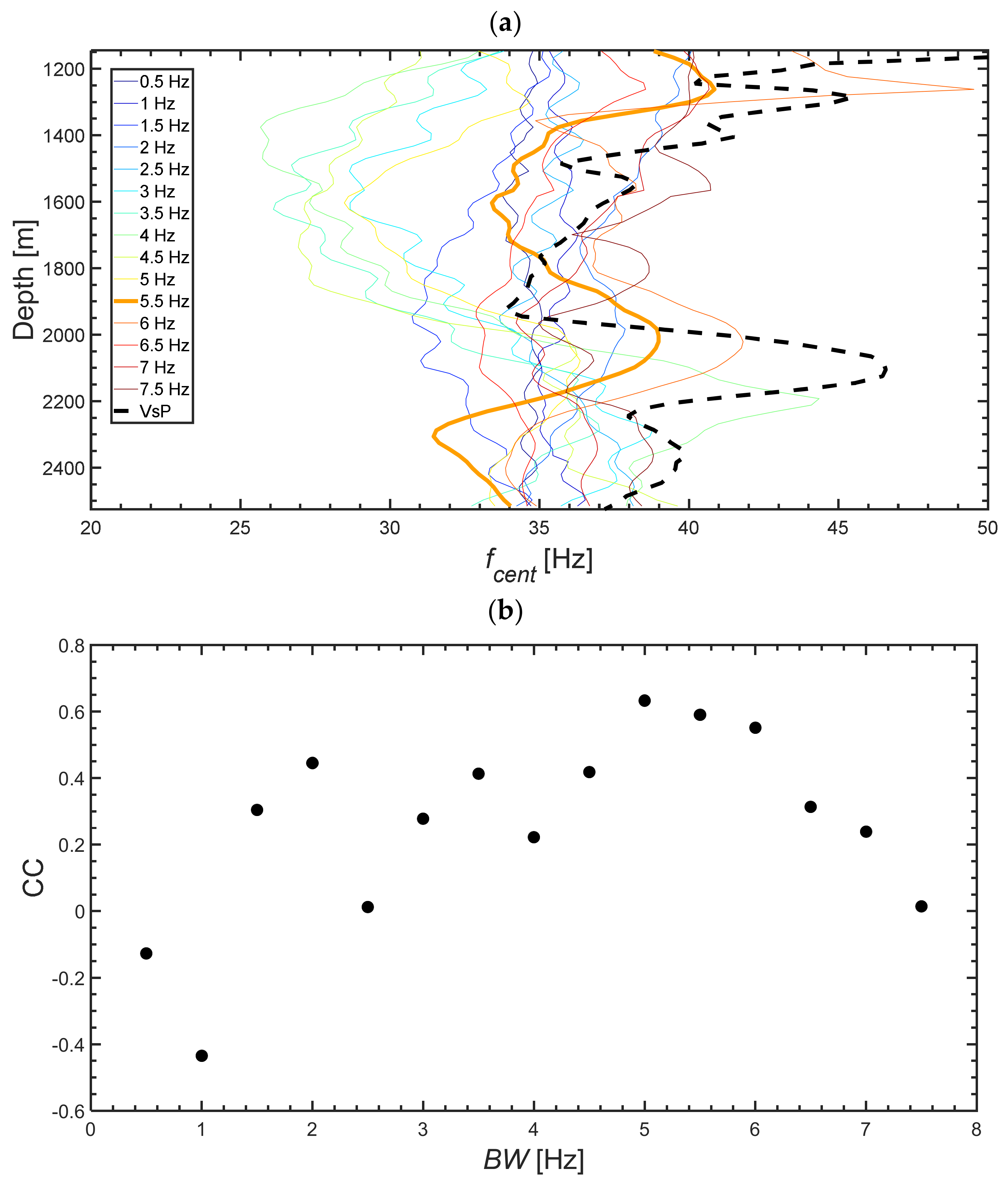
We used the linear filter proposed by Gabor [21] to create a collection of OBC spectrum traces in time domain. The bandwidth of Gabor filter was optimized by using a 3D walkaway VSP data, acquired in the same zone as surface seismic survey; Thereby, we succeed to sample the data at various known depths and made them suitable for the application of the CFS technique as in the case ZVSP;

-

The spectrum traces were converted from time to depth domain by using sonic log as a velocity model;

-

Estimation of $Q^{-1}$ by applying CFS method on traces recorded by geophones with minimum offset at each geophone line;

-

Perform linear regression of $Q^{-1}$ versus offset to calculate the intercept, which corresponds to zero offset attenuation.

The workflow developed in this study provides a high-resolution attenuation profiles with a stability and accuracy that can be checked and obtained with the assistance of VSP data. Such performance cannot be reached by the conventional methods, as the one used in the aforementioned studies.

In this study, seismic wave attenuation was not used for EOR monitoring, due to lack of seismic data during production. Nevertheless, this study provides a workflow for estimating seismic attenuation and shows the advantage of using seismic wave attenuation in delineating the zones with high oil content and fractures density, which is crucial for EOR studies.

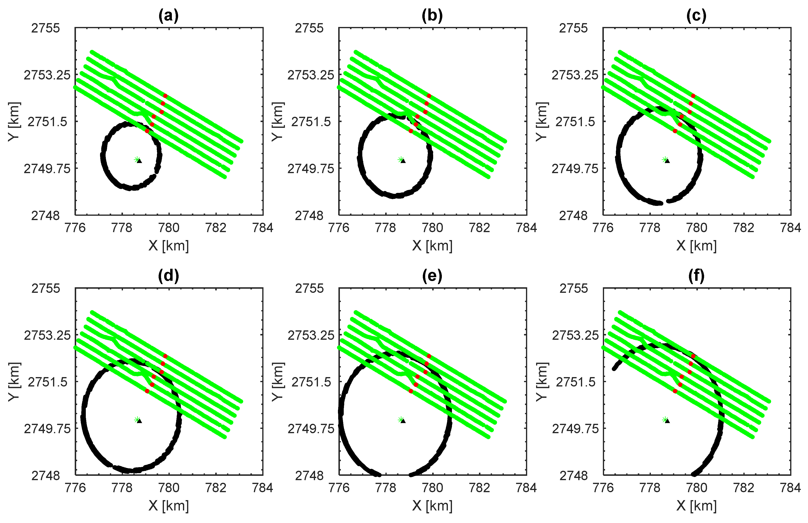
2. Study Area and Field Data

The area is one of the offshore oilfields belonging to the emirate of Abu Dhabi, United Arab Emirates (Figure 1). Its structure is an anticline with a gentle dip, having the highest magnitude in the north and northeast, where the average dip is about 2.5°. The stratigraphy of the oilfield mainly consists of Mesozoic–Cenozoic carbonates. The reservoir zones are stacked sections of porous and shallow water carbonates of the Lower Cretaceous Thamama Group.

A two-component 3D OBC seismic survey was carried out over the oilfield from 2000 to 2001. The full-fold area of the survey was 1505 km². However, in this study we focused on an area of 3 km radius around the wellhead where the 3D VSP survey was acquired (Figure 2). A series of parallel receiver cables were laid down on the seabed with sensor groups at every 50 m. The source lines were orthogonal to the receiver cables at 100 m line spacing and 25 m shot spacing on each line. For each group, hydrophone and vertical geophone data were recorded. The air gun used as source to generate data were placed 5 m below the sea surface in most of the acquisition area, and 3 m for most shallow water areas. In the shallowest area, the source was raised to 2.5 m.

The raw 3D OBC data contain an acceptable level of noise with an average magnitude of $1 \mu \mathrm{bar}$ on the hydrophones (Figure 3a) and double on the geophones (Figure 3b). The receiver lines were orientated parallel to the direction of the strongest currents to reduce the ambient noise levels. The strongest noise in the data is the dispersive ground-roll events that have velocities of around 900 ms⁻¹. Other dispersive surface waves have velocities of around 1500 ms⁻¹, but these waves have less overlap with the reflection energy.

In order to properly sum the hydrophone and geophone data, we converted the amplitudes of hydrophone data from pressure to velocity to be consistent with the geophone amplitudes. This was performed by performing an integration in the frequency domain:

$$\dot{X}\left(f\right)=\frac{\stackrel{‥}{X}\left(f\right)}{i\omega }$$

(1)

where $\stackrel{‥}{X}\left(f\right)$ is the original spectrum of hydrophone data, $\dot{X}\left(f\right)$ is the converted one, and $\omega =2\pi f$ is the angular frequency.

The summation of hydrophone and geophone data has highly reduced the ground-roll events and removed the ghost effect as well, which is due to the reverberation at sea surface (Figure 3c).

The 3D VSP survey was acquired in 2015 in the southwest part of the oilfield, where 18,364 shots were generated with an average spacing of 25 m and along a spiral pattern centered at the well head. The spiral arms were separated by an average radial interval of 50 m (Figure 2). The VSP data were acquired within an area with a radius of 3000 m from the wellhead. Seventy receivers 20 m apart were laid down in a slightly deviated well from the depth of 1145 m. Sonic and density logs were also acquired in the well (Figure 4).

Figure 3. Shot gathers of the closest shot to the VSP well (112 m from the wellhead) recorded by (a) hydrophones, (b) geophones deployed over six receiver lines during the 3D OBC survey, as shown in Figure 5 and (c) summation of hydrophones and geophones.

Figure 3. Shot gathers of the closest shot to the VSP well (112 m from the wellhead) recorded by (a) hydrophones, (b) geophones deployed over six receiver lines during the 3D OBC survey, as shown in Figure 5 and (c) summation of hydrophones and geophones.

Figure 4. (a) Sonic and (b) density logs acquired in the 3D VSP well. The dashed horizontal lines and the text labels indicate the tops and names of the various geological formations respectively.

Figure 4. (a) Sonic and (b) density logs acquired in the 3D VSP well. The dashed horizontal lines and the text labels indicate the tops and names of the various geological formations respectively.

Figure 5. Maps showing locations of selected VSP shots (black dots) at offsets of (a) 1300 m, (b) 1400 m, (c) 1650 m, (d) 1750 m, (e) 1850 m and (f) 2000 m from the wellhead (black triangle). In addition, also shown are 3D OBC receiver (geophones and hydrophones) lines (green dots) that recorded the data for the closest shot (green star) to the wellhead (black triangle) with a distance of 112 m. The geophones and hydrophones that have the smallest offset and closest to a VSP shot with same offset, at each receiver line are highlighted by red dots.

Figure 5. Maps showing locations of selected VSP shots (black dots) at offsets of (a) 1300 m, (b) 1400 m, (c) 1650 m, (d) 1750 m, (e) 1850 m and (f) 2000 m from the wellhead (black triangle). In addition, also shown are 3D OBC receiver (geophones and hydrophones) lines (green dots) that recorded the data for the closest shot (green star) to the wellhead (black triangle) with a distance of 112 m. The geophones and hydrophones that have the smallest offset and closest to a VSP shot with same offset, at each receiver line are highlighted by red dots.

3. Methodology

By assuming a wavelet spectrum of a Gaussian shape and a frequency-independent $Q$ model (Futterman, 1962), Quan and Harris (1997), estimated $Q^{-1}$ from two waveforms recorded at two receivers placed at depth $z_1$ and $z_2$ as follows:

$$Q^{-1}=\pi \Delta t\frac{f_c\left(z_1\right)-f_c\left(z_2\right)}{\pi {\sigma }_1^2\Delta t}$$

(2)

where ${\sigma }_1^2$ is the variance of the wavelet at the shallower depth $z_1$, $\Delta t$ is the travel time from $z_1$ to $z_2$ and $f_c$ is the centroid frequency of a recorded signal $A\left(z,f\right)$ defined as:

$$f_c\left(z\right)=\frac{{\displaystyle \underset{0}{\overset{\infty }{\mathsf{\int }}}f.A\left(z,f\right)df}}{{\displaystyle \underset{0}{\overset{\infty }{\mathsf{\int }}}A\left(z,f\right)df}}$$

(3)

The attenuation $Q^{-1}$ estimated by Equation (2), combines scattering ($Q_{sc}^{-1}$) and intrinsic attenuation ($Q_{\mathrm{in}}^{-1}$). As explained by [22], $Q_{sc}^{-1}$ can be estimated by appying the CFS technique on synthetic waveforms, generated from the convolution of the reflectivity with a unit amplitude spike. The reflectivity can be obtained by using Gouppillaud model [23], which is based on ray tracing and Z-transform performed in horizontally layered medium. The time interval $\Delta t$ in Gouppillaud model, is defined as the one-way travel time in each layer. The relationship between transmission ($T_k$) and reflection ($R_k$) responses of a wave propagating with an angular frequency $\omega$ in a medium of $k$th layer with an equal one-way travel time and a reflection coefficient $r_k$ at its top, is as follows:

$$\left\{\begin{array}{c}{T}_k\\ R_k\end{array}\right\}=\frac{1}{1+r_k}\left\{\begin{array}{cc}{e}^{i\omega {\tau }_k}& r_k{e}^{i\omega {\tau }_k}\\ r_k{e}^{-i\omega {\tau }_k}& e^{-i\omega {\tau }_k}\end{array}\right\}\left\{\begin{array}{c}{T}_{k+1}\\ R_{k+1}\end{array}\right\}$$

(4)

where $r_k$ can be calculated from the acoustic impedance obtained by multiplying the sonic and density logs (Figure 4), and ${\tau }_k$ is the two-way travel time of the $k\mathrm{th}$ layer.

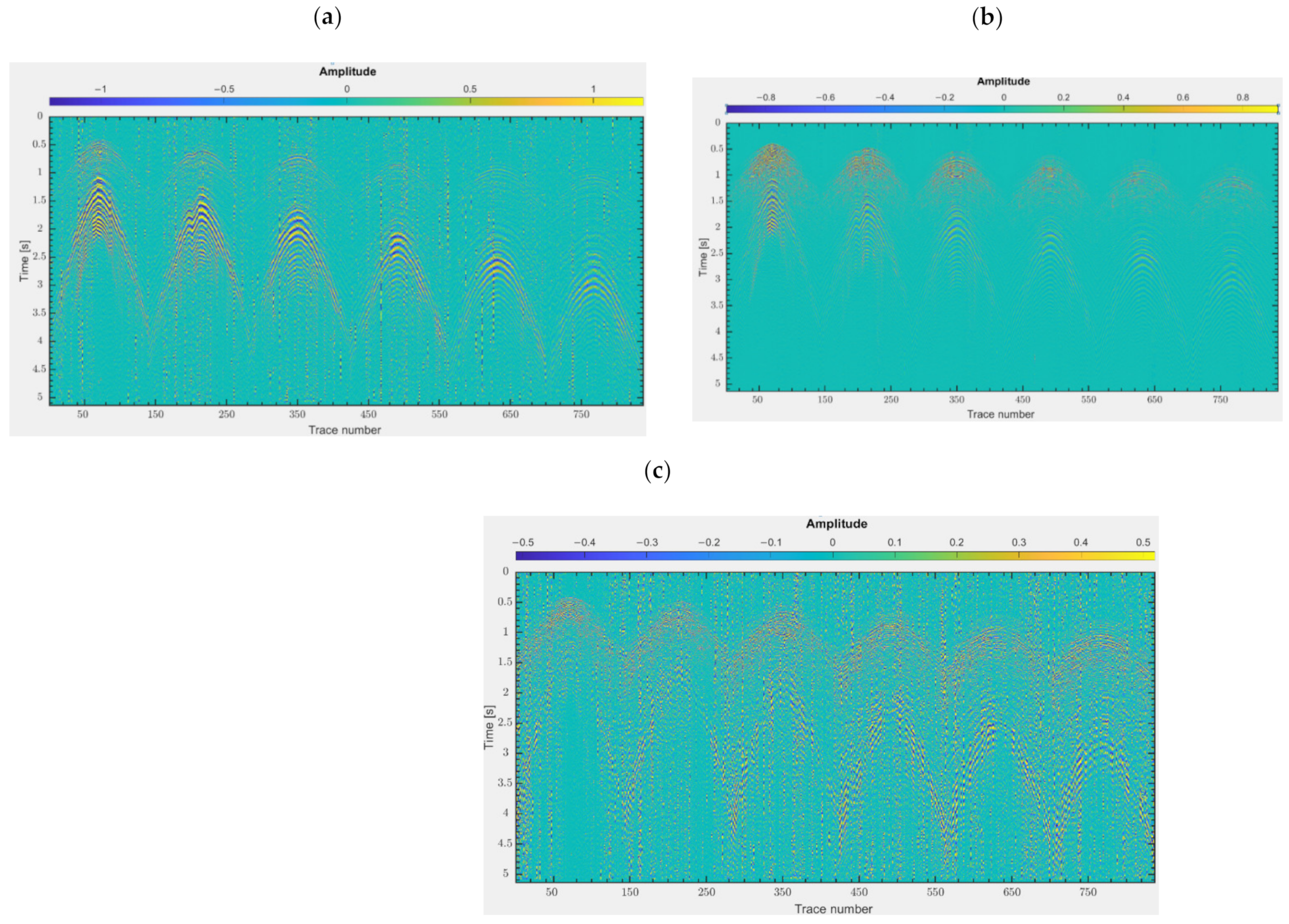
4. Attenuation Estimation from OBC Data

4.1. Workflow

A workflow (Figure 6) was developed to overcome the limitations of estimating seismic attenuation from OBC data, and to validate the calculated attenuation profiles. According to Equation (2), application of the CFS technique requires that for a given seismic shot, the spectrum must be sampled at different depths, as VSP data which are acquired at receivers placed along the vertical direction (Figure 7a). However, OBC data are acquired at receivers laid along the seafloor, which does not enable a spectrum record at different depths. This makes the application of CFS technique for a direct estimation of attenuation from OBC waveforms, not possible. In order to overcome this limitation, a collection of spectra at different depths were generated from each single seismic trace, by applying Gabor transform which is a short time Fourier transform with a Gaussian filter [21]. The Gabor transform of a signal $f\left(t\right)$ is defined by the following formula:

$$F_G\left(\omega ,\tau \right)=FT\left(f\left(t\right)W\left(t-\tau \right)\right)={\displaystyle {\mathsf{\int }}_{-\infty }^{\infty }f\left(t\right)e^{-\frac{1}{B{W}^2}{\left(t-\tau \right)}^2}}{e}^{-j\omega t}dt$$

(5)

where $FT$ indicates Fourier transform, $W$ the Gaussian filter around the time, $BW$ is the filter width and is the angular frequency.

Subsequently, a conversion from time to depth domain (Figure 7b) by using a sonic log acquired at the 3D VSP well along with a density log (Figure 4). The use of the sonic log is justified by its high depth-resolution and by the slight lateral stratigraphy changes of the subsurface.

As shows Equation (5), Gabor transform is strongly dependent on the band filter width ($BW$), which makes the generated spectra strongly dependent on $BW$. In order to correctly choose $BW$, we selected the closest 3D OBC seismic shot to the wellhead, then extracted the waveforms generated by this shot and recorded at the geophones and hydrophones that have the smallest offset at each of six receiver lines (Figure 5). According to the principal of propagation reciprocity, the waveforms extracted from the OBC data recorded at the selected geophones/hydrophones and from the 3D VSP data generated by the shots very close to the selected geophones/hydrophones (Figure 5) should be similar, and hence similar frequency profiles also. Based on that, we applied Gabor transform on the 3D OBC data by choosing a BW that produces similar OBC and VSP centroid frequency profiles. The centroid frequency profiles of the VSP and OBC seismic waveforms show the best correlation at a filter width of 5.5 Hz (Figure 8).

Eventually we obtained a $Q^{-1}$ profile at the six offsets after applying the CFS technique (Equation (2)) on the $Q^{-1}$ profiles of the waveforms acquired by the geophones and hydrophones with minimum offset at each of the six receivers. By analyzing $Q^{-1}$ cross-plots versus offset at several depths, we realized that the linear regression is the best model to fit the variation of $Q^{-1}$ with offset. Therefore, the intercept of the linear regression at each depth corresponds to the magnitude of $Q^{-1}$ at zero offset. Therefore, attenuation profile at each OBC shot position was obtained (Figure 9).

The comparison of zero offset $Q^{-1}$ with the one estimated from zero offset VSP data shows a good similarity (Figure 10). The good similarity of the $Q^{-1}$ profiles are expected since they were obtained at similar location and in the same frequency range (3–70 Hz). Such similarity also suggests that a linear relationship of $Q^{-1}$ with offset is reasonable. However, differences between the $Q^{-1}$ magnitude of OBC and VSP profiles can be noticed, which makes our study more qualitative than quantitative. Furthermore, there is a shift between $Q^{-1}$ peaks around the depth of 2000 m, which might be due to errors in velocity.

As mentioned above, the scattering $Q_{sc}^{-1}$ is obtained by applying the CFS method on synthetic seismograms. The 1D density and sonic logs were used to estimate the reflectivity of the medium by using Equation (4). In order to obtain $Q_{sc}^{-1}$ in the same frequency range as $Q^{-1}$, a band pass filter (3–70 Hz) were applied on the generated seismograms. Overall, the $Q_{sc}^{-1}$ profile shows high magnitudes (Figure 11a) which explains the high magnitudes of $Q^{-1}$. The heterogeneous nature of carbonate subsurface of Abu Dhabi, explains the high magnitudes of $Q_{sc}^{-1}$. The heterogeneity and the complex nature of the oilfield is notable through the high variation of velocity with depth (Figure 11b). Schoenberger and Levin [24] suggested that $Q^{-1}=Q_{in}^{-1}+Q_{sc}^{-1}$, meaning that by subtracting scattering from the total attenuation, the intrinsic can be obtained separately. However, it is difficult to prove this assumption, especially in complex media such as carbonates and in the case of non-zero offset data. Therefore, for sake of error we did not apply the separation between $Q_{sc}^{-1}$ and $Q_{in}^{-1}$ as suggested by [24]. Therefore, any interpretation related intrinsic attenuation in this study is based on the comparison between $Q^{-1}$ and $Q_{sc}^{-1}$.

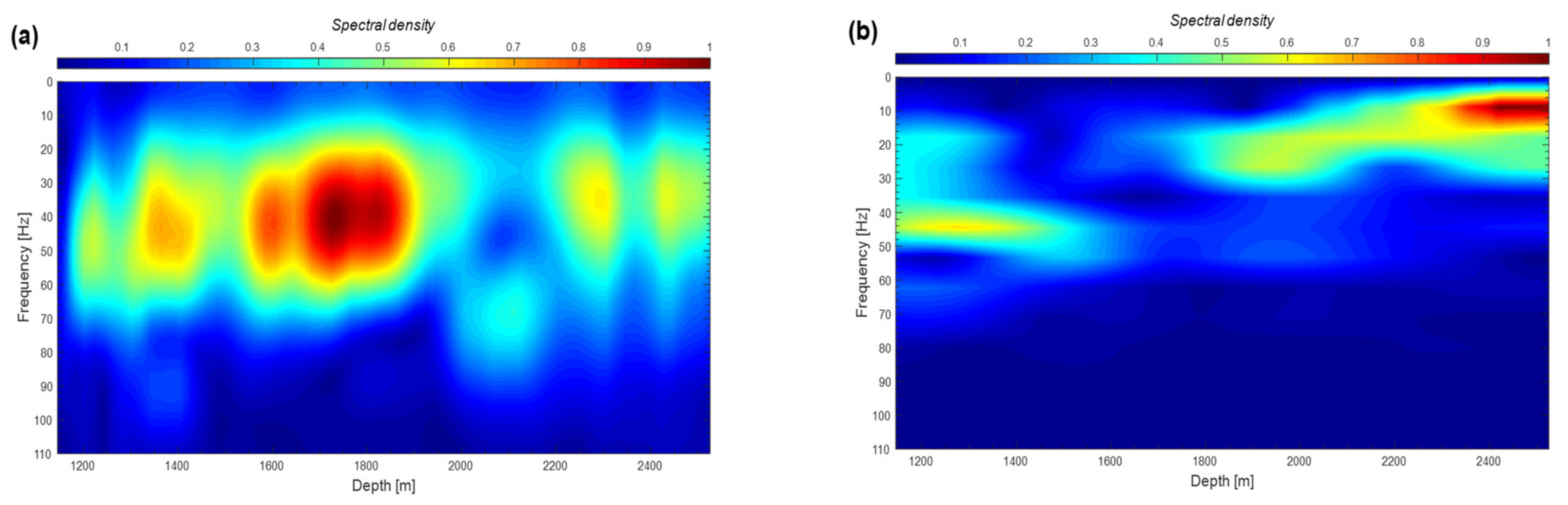
4.2. Estimation of Attenuation Profiles

By performing Gabor transform with a $BW$ of 5 Hz and estimating the zero offset $Q^{-1}$ from linear regression as shown in the workflow, 3D attenuation volumes were obtained from hydrophone, geophone data, and their summation. The results are displayed by a succession of 2D attenuation profiles obtained at selected source lines (Figure 12 and Figure 13).

We notice a good qualitative similarity between the $Q^{-1}$ profiles obtained from hydrophone (Figure 12b–d), geophone (Figure 13a,c,e) and summation (Figure 13b,d,f) data. However, the magnitude of the attenuation estimated from the hydrophone data are higher than those obtained from the other two datasets. This might be due to the noise effect, which is more prominent in the geophone and summation data than in the hydrophone data. Furthermore, due to shallow sea bottom, the wavelength is larger than the water depth (6 m–20 m), which makes reverberation removal difficult. Slight lateral variation can be observed on the 2D attenuation profiles, while the vertical variation is much significant.

The high attenuation anomalies noticed in Simsima, Fiqa and Nahr Umr Formations are due to high scattering in these formations (Figure 11a). This is in agreement with [25], where the high attenuating nature of these formations in some oilfields of Abu Dhabi was reported. The reservoir zones display high attenuation and moderate scattering, which lets us suggest that the attenuation is dominated by the intrinsic.

5. Discussion

By performing Gabor transform and a linear regression of $Q^{-1}$ with offsets, we obtained an attenuation profile at each source location used to generate the OBC data. Overall, the attenuation accuracy is reasonable, where the R-squared of the linear regression is more than 0.5 for all sources and more than 0.8 for many sources.

The attenuation magnitude shows a slight lateral variation along source lines, compared to the vertical direction. This is in agreement with seismic sections (Figure 14a) which show slight lateral variation in amplitudes. A recent velocity model obtained from a full waveform inversion (FWI) [26] generated from VSP data acquired along an azimuth of 56°, also revealed a much smaller variation of velocity in the lateral direction than in the vertical one (Figure 14b). It can be noticed that the attenuation model obtained at the same azimuthal direction (56°), displays more lateral variation than the velocity model (Figure 14c). This demonstrates the higher sensitivity of attenuation than velocity to the variation of petrophysical and lithological properties. Such sensitivity might be useful for enhancement oil recovery studies, since it can help to delineate the zones with great hydrocarbon potential, which are usually noticed by their high intrinsic attenuation anomalies.

Seismic wave attenuation was suggested as a direct detector of oil and gas, in several previous studies carried out in sandstone [27,28]. However, for subsurfaces dominated by carbonate lithology, as in the case of this study, it is still too early to consider attenuation as a direct indicator of hydrocarbon. This is because of the complex texture of carbonate media, resulting in difficulty in the understanding of attenuation mechanisms and in their estimation with reasonable acuuracy. Nevertheless, in the case of this study, the reservoir zones are clearly identifiable by their high attenuation anomaly, whereas scattering has moderate magnitudes in these zones (Figure 11). Hence, we suggest that in the reservoir zones, energy losses are dominated by intrinsic attenuation, which is the result of fluid-related mechanisms, such as WIFF mechanism known to be significant in the reservoir zones. There are two types of WIFF mechanism: global and squirt flow. The former is important in highly porous and permeable rocks [29,30], while the latter is more present in fractured media [31,32]. The high fracture density [8] and porosity in our reservoirs suggest the co-existence of global and squirt flow mechanisms. Bouchaala, et al. [33] who studied seismic attenuation in a resevoir of one of Abu Dhabi oilfields, made the evidence of the existence of global flow mechanism in porous and free-fractures zones, and of squirt flow in dense and fractured zones.

Some formations above the reservoir zones also have high attenuation anomalies, such as Nahr Umr, Salabikh, and Simsima Formations (Figure 12b,d). However, opposite to reservoir zones where fluid-related mechanisms are important, the scattering is the dominant attenuation component in these formations (Figure 11a). The high magnitudes of scattering reflect the heterogeneous and complex lithology of these formations. Indeed, fine layering is the main cause of high scattering at the base of middle cretaceous Nahr Umr Formation which is made of variegated shales and occasional thin limestones [34]. Many full-bore formation micro-imager observations in Abu Dhabi oilfields show a pronounced thin bedding planes in Nahr Umr Formation, which is usual in shaly rocks [34,35]. The upper middle cretaceous Salabikh Formation is a sequence of three members made of highly variable succession of beds and consists of lime mudstones, soft dense argillaceous limestones with very calcareous shale interbeds [34]. Such bedding explains the high scattering in this formation. The Upper Cretaceous Simsima Formation is highly heterogeneous, and its lithology is dominated by depositional packstones, in a shallow water environment, representing a regressive sea level phase. Furthermore, Simsima Formation is an important aquifer in Abu Dhabi as well as an oil-bearing reservoir in the Shah Field [36,37]. Therefore, Simsima Formation is a favorable medium for scattering and WIFF mechanisms. A previous study performed in another oilfield located in Abu Dhabi has reported high attenuation anomalies in Simsima Formation.

The NW part of the study area displays negative attenuation values at depths between 1700 m and 1850 m and below 2400 m (Figure 12d). Mateeva [38] suggested that the most probable reason behind negative attenuation is the sensitivity of the CFS technique to the interference phenomenon caused by short wavelength upgoing waves, such as small amplitude multiples. Another reason might be the disturbance caused by noise. Decreasing the vertical resolution of $Q^{-1}$ might be a solution to obtain more stable results, and to avoid the negative magnitudes of $Q^{-1}$. However, the resolution of $Q^{-1}$ is important for its comparison with the petrophysical properties of the subsurface, which are typically acquired with a vertical resolution of 0.1524 m along the wellbore. Therefore, a compromise should be performed between the resolution and stable magnitudes of $Q^{-1}$. On this basis, the resolution of our attenuation profiles was set equals to 100 m. Furthermore, negative magnitudes of scattering were noticed, such as those around the depth of 1745 m where $Q_{sc}^{-1}=-0.04$ (Figure 11a). Liner [39] explained negative scattering by negative normal reflection coefficient $\left(R_0\right)$, which is the result of negative impedance contrast. Based on the continuity relationship $R_0+T_0=1$, the normal transmission coefficient $\left(T_0\right)$ has to be larger than one, meaning an amplification in the amplitude of transmitted waves which results in negative $Q_{sc}^{-1}$.

In this study, qualitative results were presented and the 3D variation of attenuation in the subsurface of an oilfield was shown. The results pointed out the advantages of using seismic wave attenuation for detecting and delineating, heterogeneous and fluid-saturated zones, such as reservoirs and aquifers. However, estimating attenuation from large offset 3D seismic data is still challenging, because at high offsets the interference phenomenon is important, which may reduce the accuracy of attenuation estimates.

Bouchaala, et al. [40] showed through a synthetic data with similar geometry to non-zero offset VSP data, that the error induced by the offset is noticeable at offsets higher than 2000 m. Nevertheless, for larger offsets they showed that the variation of the attenuation profile remains acceptable. The offsets used in this study vary from 20 m to 4000 m.

Furthermore, a correct separation between scattering and intrinsic attenuation can eliminate negative values of $Q^{-1}$ and enhance interpretation. However, the methodology for estimating and separating scattering from 3D seismic data is still premature and challenging.

6. Conclusions

The workflow developed in this study allowed us to apply the CFS technique on OBC seismic data, in order to estimate seismic wave attenuation. The limitation of the CFS technique due to the location of OBC receivers on the seafloor, was overcome by applying an optimized Gabor transform to create a collection of spectrum traces in the time domain, followed by a conversion from time to depth domain. The results showed high attenuation anomalies in highly saturated and heterogeneous zones, such as the reservoir zones and Simsima Formation. Such results show the advantage of using seismic wave attenuation for petroleum exploration and reservoir characterization. A slight lateral variation at each seismic line was revealed by the 2D attenuation profiles, which agrees with velocity profiles and results of full waveform inversion.

References

1. Li, K.; Chen, B.; Pu, W.; Jing, X.; Yuan, C.; Varfolomeev, M. Characteristics of Viscoelastic-Surfactant-Induced Wettability Alteration in Porous Media. Energies 2021, 14, 8454. [Google Scholar] [CrossRef]
2. Khan, U.; Zevenhoven, R.; Stougie, L.; Tveit, T.-M. Prediction of Stirling-Cycle-Based Heat Pump Performance and Environmental Footprint with Exergy Analysis and LCA. Energies 2021, 14, 8478. [Google Scholar] [CrossRef]
3. Chichinina, T.; Martyushev, D. Specific Anisotropy Properties of Fractured Reservoirs: Research on Thomsen’s Anisotropy Parameter Delta; Geomodel 2021; European Association of Geoscientists & Engineers: Amsterdam, The Netherlands, 2021; pp. 1–5. [Google Scholar]
4. Ali, M.Y.; Bouchaala, F.; Bouzidi, Y.; Takam Takougang, E.M.; Mohamed, A.A.; Sultan, A. Integrated Fracture Characterization of Thamama Reservoirs in Abu Dhabi Oil Field, United Arab Emirates. SPE Reserv. Evaluation Eng. 2021, 24, 70–720. [Google Scholar] [CrossRef]
5. Hudson, J.; Liu, E.; Crampin, S. The mechanical properties of materials with interconnected cracks and pores. Geophys. J. Int. 1996, 124, 105–112. [Google Scholar] [CrossRef] [Green Version]
6. Best, A.I.; Sothcott, J.; McCann, C. A laboratory study of seismic velocity and attenuation anisotropy in near-surface sedimentary rocks. Geophys. Prospect. 2007, 55, 609–625. [Google Scholar] [CrossRef]
7. Bouchaala, F.; Ali, M.Y.; Matsushima, J.; Bouzidi, Y.; Takam Takougang, E.M.; Mohamed, A.A.; Sultan, A. Scattering and intrinsic attenuation as a potential tool for studying of a fractured reservoir. J. Pet. Sci. 2019, 174, 533–543. [Google Scholar] [CrossRef]
8. Bouchaala, F.; Ali, M.Y.; Matsushima, J.; Bouzidi, Y.; Takam Takougang, E.M.; Mohamed, A.A.; Sultan, A. Azimuthal investigation of compressional seismic-wave attenuation in a fractured reservoir. Geophysics 2019, 84, B437–B446. [Google Scholar] [CrossRef]
9. Yang, Y.; Yin, X.; Zhang, B.; Cao, D.; Gao, G. Linearized Frequency-Dependent Reflection Coefficient and Attenuated Anisotropic Characteristics of Q-VTI Model. Energies 2021, 14, 8506. [Google Scholar] [CrossRef]
10. Wu, R.S. Attenuation of short period seismic waves due to scattering. Geophys. Res. Lett. 1982, 9, 9–12. [Google Scholar]
11. Wu, R.-S.; Aki, K. Introduction: Seismic wave scattering in three-dimensionally heterogeneous earth. In Scattering and Attenuations of Seismic Waves, Part I; Springer: Berlin/Heidelberg, Germany, 1988; pp. 1–6. [Google Scholar]
12. Pride, S.R.; Berryman, J.G.; Harris, J.M. Seismic attenuation due to wave-induced flow. J. Geophys. Res. Solid Earth 2004, 109, B1. [Google Scholar] [CrossRef]
13. Müller, T.M.; Gurevich, B.; Lebedev, M. Seismic wave attenuation and dispersion resulting from wave-induced flow in porous rocks—A review. Geophysics 2010, 75, 75A147–75A164. [Google Scholar] [CrossRef]
14. Harris, J.M.; Yin, F.; Quan, Y. Enhanced oil recovery monitoring using P-wave attenuation. In SEG Technical Program Expanded Abstracts 1996; Society of Exploration Geophysicists: Houston, TX, USA, 1996; pp. 1882–1885. [Google Scholar]
15. Spencer Jr, J.W. Viscoelasticity of Ells River bitumen sand and 4D monitoring of thermal enhanced oil recovery processes. Geophysics 2013, 78, D419–D428. [Google Scholar] [CrossRef]
16. McDonal, F.; Angona, F.; Mills, R.; Sengbush, R.; Van Nostrand, R.; White, J. Attenuation of shear and compressional waves in Pierre shale. Geophysics 1958, 23, 421–439. [Google Scholar] [CrossRef]
17. Quan, Y.; Harris, J.M. Seismic attenuation tomography using the frequency shift method. Geophysics 1997, 62, 895–905. [Google Scholar] [CrossRef]
18. Dasgupta, R.; Clark, R.A. Estimation of Q from surface seismic reflection data. Geophysics 1998, 63, 2120–2128. [Google Scholar] [CrossRef]
19. Rossi, G.; Gei, D.; Böhm, G.; Madrussani, G.; Carcione, J.M. Attenuation tomography: An application to gas-hydrate and free-gas detection. Geophys. Prospect. 2007, 55, 655–669. [Google Scholar] [CrossRef]
20. Bouchaala, F.; Guennou, C. Estimation of viscoelastic attenuation of real seismic data by use of ray tracing software: Application to the detection of gas hydrates and free gas. C R Geosci. 2012, 344, 57–66. [Google Scholar] [CrossRef]
21. Gabor, D. Theory of communication. Part 1: The analysis of information. J. Inst. Electr. Eng. 1946, 93, 429–441. [Google Scholar] [CrossRef] [Green Version]
22. Matsushima, J. Seismic wave attenuation in methane hydrate-bearing sediments: Vertical seismic profiling data from the Nankai Trough exploratory well, offshore Tokai, central Japan. J. Geophys. Res. Solid Earth 2006, 111, B10. [Google Scholar] [CrossRef]
23. Goupillaud, P.L. An approach to inverse filtering of near-surface layer effects from seismic records. Geophysics 1961, 26, 754–760. [Google Scholar] [CrossRef]
24. Schoenberger, M.; Levin, F. Apparent attenuation due to intrabed multiples. Geophysics 1974, 39, 278–291. [Google Scholar] [CrossRef]
25. Bouchaala, F.; Ali, M.Y.; Farid, A. Estimation of compressional seismic wave attenuation of carbonate rocks in Abu Dhabi, United Arab Emirates. C R Geosci. 2014, 346, 169–178. [Google Scholar] [CrossRef]
26. Takam Takougang, E.; Ali, M.Y.; Bouzidi, Y.; Bouchaala, F.; Sultan, A.A.; Mohamed, A.I. Characterization of a carbonate reservoir using elastic full-waveform inversion of vertical seismic profile data. Geophys. Prospect. 2020, 68, 1944–1957. [Google Scholar] [CrossRef]
27. Rapoport, M.B.; Rapoport, L.I.; Ryjkov, V.I. Direct detection of oil and gas fields based on seismic inelasticity effect. Lead. Edge 2004, 23, 276–278. [Google Scholar] [CrossRef]
28. Ma, R.-P.; Ba, J.; Carcione, J.M.; Zhou, X.; Li, F. Dispersion and attenuation of compressional waves in tight oil reservoirs: Experiments and simulations. Appl. Geophys. 2019, 16, 33–45. [Google Scholar] [CrossRef]
29. Assefa, S.; McCann, C.; Sothcott, J. Attenuation of P-and S-waves in limestones. Geophys. Prospect. 1999, 47, 359–392. [Google Scholar] [CrossRef]
30. Gurevich, B.; Zyrianov, V.B.; Lopatnikov, S.L. Seismic attenuation in finely layered porous rocks: Effects of fluid flow and scattering. Geophysics 1997, 62, 319–324. [Google Scholar] [CrossRef]
31. Marketos, G.; Best, A. Application of the BISQ model to clay squirt flow in reservoir sandstones. J. Geophys. Res. Solid Earth 2010, 115, B6. [Google Scholar] [CrossRef] [Green Version]
32. Jakobsen, M.; Chapman, M. Unified theory of global flow and squirt flow in cracked porous media. Geophysics 2009, 74, WA65–WA76. [Google Scholar] [CrossRef] [Green Version]
33. Bouchaala, F.; Ali, M.Y.; Matsushima, J. Attenuation study of a clay-rich dense zone in fractured carbonate reservoirs. Geophysics 2019, 84, B205–B216. [Google Scholar] [CrossRef]
34. Fox, A.; Brown, R. The geology and Reservoir Characteristics of the Zakum Oil Field, Abu Dhabi; Regional Technical Symposium; Society of Petroleum Engineers: Dhahran, Saudi Arabia, 1968. [Google Scholar]
35. Nguyen, V.X.; Abousleiman, Y.N.; Hoang, S. Analyses of Wellbore Instability in Drilling through Chemically Active Fractured Rock Formations: Nahr Umr Shale. In Proceedings of the SPE Middle East Oil and Gas Show and Conference, Manama, Bahrain, 11–14 March 2007; Society of Petroleum Engineers: Manama, Bahrain, 2007. [Google Scholar]
36. Kannan, J. Successful ESP Operation ADCO-SHAH FIELD; Abu Dhabi International Petroleum Exhibition and Conference; OnePetro: Abu Dhabi, United Arab Emirates, 2015. [Google Scholar]
37. Evans, G.; Kirkham, A. A geological excursion to Jebels Rawdah, Buhays and Faiyah. Tribulus 2016, 24, 85–93. [Google Scholar]
38. Mateeva, A.A. Thin horizontal layering as a stratigraphic filter in absorption estimation and seismic deconvolution. PhD Thesis, Colorado School of Mines, Golden, CO, USA, 2003. [Google Scholar]
39. Liner, C.L. Long-wave elastic attenuation produced by horizontal layering. Lead. Edge 2014, 33, 634–638. [Google Scholar] [CrossRef]
40. Bouchaala, F.; Ali, M.; Matsushima, J. Estimation of seismic attenuation in carbonate rocks using three different methods: Application on VSP data from Abu Dhabi oilfield. J. Appl. Geophy 2016, 129, 79–91. [Google Scholar] [CrossRef]
Figure 1. Map of Abu Dhabi oilfields. The oilfield of this study is denoted by nearby red text.
Energies 15 00534 g001
Figure 2. A basemap showing the shot positions of the 3D OBC seismic and 3D VSP surveys. In addition, also shown are the positions of the downhole receivers, wellhead and a line with an azimuth of 56° passing by the center of the VSP survey.
Energies 15 00534 g002
Figure 6. The proposed workflow to estimate the filter width of Gabor transform and to validate Q−1 profile at the well location.
Energies 15 00534 g006
Figure 7. Spectrum of (a) VSP data recorded at an offset of 1300 m and (b) those obtained after applying Gabor transform with a filter width of 5 Hz and time to depth conversion, on OBC seismic data recorded at an offset of 1300 m.
Energies 15 00534 g007
Figure 8. Centroid frequencies of: (a) OBC seismic spectra obtained at different values of the filter width ( B W ) (solid curves) and VSP spectrum (dashed curve), centroid frequency curves of VSP and B W = 5.5   Hz are highlighted by thick lines; (b) coefficient of cross-correlation between OBC and VSP centroid frequency curves at different values of BW.
Energies 15 00534 g008
Figure 9. Variation of attenuation Q 1 with offset. Q 1 was estimated from hydrophones with minimum offsets at the receiver lines as shown in Figure 5. Blue dashed line is the best-fit linear regression line. R2 is the determination coefficient. R 2 = 1 i = 1 N y i Q i 1 2 i = 1 N y i Q i 1 ¯ 2 , where y i is the attenuation calculated from the equation of the linear regression y = 2.44 × 10 4 x + 0.43053 , Q i 1 is the input attenuation estimated from the 3D OBC seismic data, and N (=6) is the number of hydrophones.
Energies 15 00534 g009
Figure 10. Zero offset Q 1 profiles obtained from 3D VSP data (black) and from a linear fitting of Q 1 estimated from 3D OBC seismic data (red), generated by the closest shot (the green star in Figure 5) to the wellhead (the black triangle in Figure 5) and recorded by hydrophones that have the smallest offsets (the red dots in Figure 5).
Energies 15 00534 g010
Figure 11. (a) Scattering and (b) the relative variation of velocity. The dashed horizontal lines and the text labels indicate the tops and names of the various geological formations respectively.
Energies 15 00534 g011
Figure 12. (a) Location of the 3D OBC shots (black dots). The red circle delimits the acquisition zone of 3D VSP survey, which has a maximum offset of 3000 m from the wellhead (red dot). The green lines show location of the 2D normalized and smoothed attenuation profiles estimated from hydrophone data displayed in (b,d,f) and R-squared of the linear regression displayed in (c,e,g). The solid horizontal lines and the text labels indicate the tops and names of the various geological formations respectively.
Energies 15 00534 g012
Figure 13. The 2D smoothed attenuation profiles obtained from geophone (a,c,e) and the summation of hydrophone and geophone (b,d,f) data generated by the shots belonging to the source lines highlighted by green color Figure 12a. The solid horizontal lines and the text labels indicate the tops and names of the various geological formations respectively.
Energies 15 00534 g013
Figure 14. (a) Post-stack migrated section of the 3D VSP along an azimuth of 56°. (b) Smoothed compressional velocity profile obtained from full waveform inversion of the VSP data [26]. (c) Normalized and smoothed attenuation profile obtained from hydrophone data. All the profiles were obtained along an azimuth of 56° as highlighted in magenta color in Figure 2. The dashed horizontal lines and the text labels indicate the tops and names of the various geological formations respectively, while the black dots indicate the downhole receivers.
Energies 15 00534 g014
Publisher’s Note: MDPI stays neutral with regard to jurisdictional claims in published maps and institutional affiliations.