
Assessing Feature Importance for Short-Term Prediction of Electricity Demand in Medium-Voltage Loads


1
Department of Mathematics and Computer Science, University of Cagliari, 09124 Cagliari, Italy
2
Department of Electrical and Electronic Engineering, University of Cagliari, 09123 Cagliari, Italy
*
Author to whom correspondence should be addressed.
Energies 2022, 15(2), 549; https://0-doi-org.brum.beds.ac.uk/10.3390/en15020549
Submission received: 18 November 2021
/
Revised: 25 December 2021
/
Accepted: 5 January 2022
/
Published: 13 January 2022
(This article belongs to the Special Issue Machine Learning and Complex Networks Analysis)
Abstract
:The design of new monitoring systems for intelligent distribution networks often requires both real-time measurements and pseudomeasurements to be processed. The former are obtained from smart meters, phasor measurement units and smart electronic devices, whereas the latter are predicted using appropriate algorithms—with the typical objective of forecasting the behaviour of power loads and generators. However, depending on the technique used for data encoding, the attempt at making predictions over a period of several days may trigger problems related to the high number of features. To contrast this issue, feature importance analysis becomes a tool of primary importance. This article is aimed at illustrating a technique devised to investigate the importance of features on data deemed relevant for predicting the next hour demand of aggregated, medium-voltage electrical loads. The same technique allows us to inspect the hidden layers of multilayer perceptrons entrusted with making the predictions, since, ultimately, the content of any hidden layer can be seen as an alternative encoding of the input data. The possibility of inspecting hidden layers can give wide support to researchers in a number of relevant tasks, including the appraisal of the generalisation capability reached by a multilayer perceptron and the identification of neurons not relevant for the prediction task.
1. Introduction
Monitoring systems for intelligent distribution grids allow measurements to be gathered from the field and the state of a distribution system to be estimated over time. In particular, distribution system state estimation (DSSE) relies on different sources of information to obtain an accurate picture of the network status. The design of new approaches able to deal with DSSE challenges requires to process both real-time measurements and pseudomeasurements [1]. In particular, the former are obtained from instruments such as smart meters (SMs), distribution-level phasor measurement units and smart electronic devices, whereas the latter are typically predicted using proper models and algorithms. Pseudomeasurements are values of absorbed and generated power, predicted with a given anticipation, e.g., an hour or a day ahead, depending on the availability of historical and past data. Since real-time measurements are scarce in distribution grids, even considering rapidly changing scenarios and the ongoing upgrade of monitoring infrastructures, pseudomeasurements are and will be essential to achieve observability. Thus, a typical objective of the prediction module is to predict the behaviour of power loads and generators with a suitable accuracy. Further, the activity of predicting power (with time horizons that can vary from a few hours to days or weeks) is of fundamental importance to ensure a good management of a distribution system. In a fast changing scenario, as it is the so-called smart grid, where high penetration of renewable generation and of distributed energy resources is likely, the erratic behaviour of these sources and of new electric loads makes the prediction even more challenging [2].
Many proposals have been made over time in this research field. Without claiming to be exhaustive, some of them are recalled hereinafter, with focus on short-term forecasting. Wu et al. [3] implemented a robust state estimator for medium voltage distribution networks. In particular, two multilayer perceptrons (MLPs, hereafter) were trained to forecast nodal active and reactive power of medium-voltage (MV) nodes, with the goal of providing pseudomeasurements to the closed-loop state estimator. To this end, MLPs were retrained when a new load time series was made available. Manitsas et al. [4] proposed a system that uses MLPs to realign the average load profiles with the actual power flow measurements available at the network substation. Hayes et al. [5] used an MLP to forecast active power value one day ahead, based on MV load information obtained through low-voltage SM measurements, together with weather- and time-related information. Carcangiu et al. [6] used an MLP to generate pseudomeasurements for distribution system state estimation. In particular, an MLP was trained to predict, one step ahead, the active and reactive power demands at each medium-voltage node. Exogenous variables were used as inputs of the predictive model, together with historical load information. In [7], five machine learning methods (i.e., MLPs, support vector machines, radial basis functions, decision trees and Gaussian processes) were compared in the task of predicting the active power consumption for the next 100 h. The comparative work pointed out that MLPs performed better than other methods. In [8], genetic programming was applied to predict short-term load forecasting. Load series of the same time point, at different days, were chosen to train the system. Aprillia et al. [9] used random forests to predict the load behaviour on a daily basis. The authors proposed a statistical load forecasting system, which makes use of quantile regression random forests, probability maps and risk assessment indexes. Deep learning techniques have also been successfully applied to the problem of load forecasting. Among many proposals, let us recall the work of Hong et al. [10], who proposed a forecasting method (tailored for individual users) that uses deep neural networks to learn the spatio-temporal correlations among different kinds of electricity consumption behaviours. Chen et al. [11] proposed a model aimed at predicting short-term electric loads. In particular, a custom deep residual network was devised and implemented to improve forecasting based on historical power data. Moreover, a two-stage ensemble strategy was used to enhance the generalization capability of the proposed model. To forecast the 24-hour-ahead values of the system load at city level, Bashari et al. [12] used long short-term memory to analyse the historical load sequences, whereas a deep neural network was applied to map the predicted meteorological parameters to the system load. For further information on short-term load forecasting, the interested reader may also consult the review articles of Wang et al. [13] and of Hippert et al. [14].
Within the groundwork of predicting the demand for electricity consumption for an MV-aggregated load over the next hour using heterogeneous information, a relevant task is how to filter out ineffective features while retaining the most important ones. This issue becomes of fundamental importance when the number of features grows—the more features, the more problematic the solution. A powerful strategy aimed at contrasting this issue is feature selection (FS), which is the process of selecting a set of representative features required (or at least helpful) in the task of building the forecasting model. A simple, yet effective, way to deal with this problem consists of ranking the available features according to their importance with respect to the variable being predicted, then use the most effective ones for training a predictive model. This solution falls into the category of filter methods, which do not account for the interaction amongst features. Relevant examples in this category are the test, Fisher score, Pearson correlation coefficient and variance threshold. Wrapper methods are another general category of FS techniques, which are able to detect the interactions amongst variables. Let us recall here three representative algorithms—i.e., recursive feature elimination, sequential FS and genetic algorithms. The cited techniques are combined in the so-called embedded methods, which are able to combine their advantages while dealing, to some extent, with their drawbacks. A learning algorithm takes advantage of its own variable selection process and performs FS and classification simultaneously. Classical examples of this category are random forests and elastic net.
Without claiming to be exhaustive, some relevant works that make use of FS techniques and algorithms in the field of energy load demands are briefly recalled hereinafter. Rana et al. (2012) [15] proposed an FS approach for very short-term electricity load forecasting. After an initial selection based on weekly and daily load patterns, a further selection was performed by using two filters—i.e., RReliefF [16] and mutual information. In a subsequent work, Rana et al. showed that correlation-based FS [17] and mutual information were able to identify a small set of informative lag variables, that resulted in good quality predictions of intervals of electricity demands. In 2019, Gao et al. [18] observed that many factors affected short-term electric load and the superposition of these factors led to it being non-linear and non-stationary. To deal with the complexity of the model to be learned, the authors proposed a solution based on an empirical mode decomposition-gated recurrent unit, called EMD-GRU, which performs a preprocessing step that enforces filter methods based on Pearson correlation. Eseye et al. (2019) [19] proposed an FS approach for accurate short-term electricity demand forecasting in distributed energy systems. This proposal relies on binary genetic algorithms to perform the FS process, whereas Gaussian process regression is used for measuring the fitness score of the features. A feed-forward artificial neural network is then used to evaluate the forecast performance of the selected predictor subset. Kim et al. (2020) [20] proposed a long–short-term memory-based model to forecast the electric consumption of VRF systems according to the state information and control signals. The authors implemented two methods to overcome the difficulties of properly handling the depth of the network and the number of neurons per hidden layer. The first one is relevant, being an FS method that makes use of the Pearson correlation coefficient and random forests to assess feature importance. In 2020, Sankari and Chinnappan [21] integrated several kinds of FS techniques (i.e., fast correlation-based filter, mutual information and RReliefF) to improve short term load forecasting. Afterwards, they used cluster-based FS to group similar load patterns and eliminate the outliers. A long–short-term memory was then trained on the given data and compared against other relevant models. As expected, the performance of the proposed forecasting model was improved, due to the preprocessing step based on FS. The experimental results showed that the models with selected features (especially the one with RReliefF) outperformed the other models.
In this article, an FS technique that falls under the umbrella of filter methods is proposed and used in the task of predicting the demand of electricity consumption. The technique, based on measures [22], provides information about the effectiveness of each input feature with respect to the target. Furthermore, the same technique is also used on the hidden layers of the adopted MLP model, thus putting into practice a kind of multivariate analysis. This capability should not be surprising, as any hidden neuron is made, in fact, by combining the input features. This consideration makes clear that MLPs were selected as reference model beyond the fact that they are very effective machine learning tools. The advancement proposed in this article consists of showing that (i) diagrams can be successfully used to perform FS and that (ii) the impact of FS can be directly investigated using diagrams by looking at the patterns that arise inside MLPs. The experimental results highlight the effectiveness of the proposal in a comparative setting, where the adopted model was first trained on all available features and then on selected ones. To the best of our knowledge, this is the first time that diagrams are used in a task regarding the prediction of electrical load demands. The remainder of the article is organised as follows: Section 2 is aimed at illustrating the characteristics of data sources, the techniques adopted to perform data encoding and the algorithms used to perform model training; Section 3 summarizes experiments and the corresponding results; and Section 4 depicts conclusions and future work.
2. Materials and Methods
This section ranges over different aspects of the proposal. First, some notes on the characteristics of the data source are given, pointing in particular to the available features and to the adopted encoding technique; then, the tools and measures adopted to assess feature importance are sketched; finally, the algorithm used to train the machine learning models is briefly depicted.
2.1. Data Sources and Their Encoding
The data used in this research comes from two different sources, i.e., residential and enterprise active power consumption data recorded from 14 July 2009 to 31 December 2010 by customers involved in the Electricity Smart-Metering Customer Behaviour Trials and made available by the Commission for Regulation of Utilities (formerly Commission for Energy Regulation) [23]. The former regards the loads on a family basis, whereas the latter regards the loads of small- and medium-size enterprises (SMEs). Consumption data were recorded from customers’ SMs equipped with different communication technologies at various distribution network locations in Ireland (particularly in Limerick and Cork areas); they come, originally, from 6445 customers, of which 4225 were households and 485 SMEs. The trials were managed by Electricity Supply Board (ESB), a state-owned electricity company. The dataset followed a rigorous assessment process, from installation to data collection and analysis, thus making it well suited for further research. In addition, it was possible to associate, with a reasonable accuracy, weather data collected from the Irish Meteorological Service [24] to integrate the active power dataset. In the dataset, SME customers are also indicated as belonging to different sectors, such as entertainment (hotels, sporting facilities and restaurants), industry, offices and retail premises. Among the available SMs, 3423 residential and 287 SME customers completed the trial, thus having a full measurement record for the whole period. As a general comment, the two types of load were quite different, since household consumption is less regular, depending on the residents’ lifestyle. SME loads follow instead regular activity during the week, with different patterns in working days and weekends.
This paper focuses on active power prediction at MV nodes, which is particularly useful to define pseudomeasurements for DSSE. To this end, two equivalent MV loads were obtained aggregating SM readings, while keeping the distinction between residential and enterprise data to investigate their peculiarities. In particular, 537 residential customers (randomly selected among those that had completed the trial) and 46 enterprise customers were used to define two active power datasets. The active power ranges were 74–653 kW and 180–963 kW, respectively, for the two time series. Both datasets share the same kind of features and were encoded in the same way. Each dataset follows a standard 2D representation, in which a row corresponds to a data instance and a column to a feature. For both residential and enterprise data, an instance contains 11 values, recorded over time or calculated. The corresponding features are reported in Table 1.
The temperatures of dry bulb, wet bulb and dew point are important for determining the state of humid air, including the water vapour content and the sensible and latent energy (enthalpy) in the air. The dry bulb temperature basically refers to the ambient air temperature (its name derives from the fact that the temperature is provided by a thermometer not affected by the humidity of the air). The wet bulb temperature is the lowest temperature that can be reached under current ambient conditions by the evaporation of water only; it can be measured using a thermometer with the bulb wrapped in a light wet (muslin) fabric. The dew point is the temperature at which water vapour begins to condense out of the air (i.e., the temperature at which the air becomes completely saturated); above this temperature, moisture remains in the air. Note that, for reasons of privacy, no precise location was associated with individual SMs. Moreover, temperature and humidity values measured by different weather stations located in the same area were averaged and used to define the weather variables corresponding to the power data.
The available datasets underwent few encoding steps. The first activity was aimed at generating two new datasets, from residential and enterprise customers, by sliding a time window over the available data. This technique allows past data of arbitrary length to be embedded into a single instance, depending on the user needs. In this work, the window length was set to cover the past 7 days. Considering the granularity of an hour, the number of resulting features was . Afterwards, the features related to temperature and air humidity underwent Gaussian scaling. Then, all features were constrained in the interval by enforcing MinMax scaling. As for the target, it was encoded according to the values of two consecutive loads. First, each load underwent MinMax scaling in the interval . Let be the difference between the load value measured at time k and the one measured at time (note that falls within the range , as load values are scaled in ). The last transformation consisted of yielding a classification problem. To this end, each was projected into a nominal range of three labels, i.e., lower, equal and greater (encoded as , 0 and ).
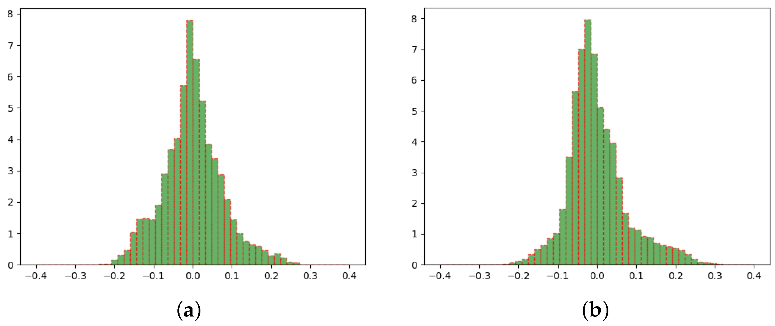
Figure 1 reports the hourly network dynamics, for both residential and enterprise customers. As data underwent MinMax scaling in the interval , in principle, both time series were bound by the interval . However, due to the dynamics of the underlying process, the actual range was approximately bound by the interval . Given the shape of the resulting distribution and the willingness to partition the data into three balanced subsets, the threshold associated to equal was . Note that defining a small interval for “equality” is also compliant with the need of predicting changes (no matter if increasing or decreasing). In so doing, two subsequent load values were considered approximately equal when . For more extreme differences, the next load values were considered lower or greater than the previous one, depending on the sign of the difference.
2.2. Tool Adopted for Feature Importance Analysis
As pointed out, a feature importance analysis was performed by means of diagrams, which are a variant of ROC curves (see, for example, Bradley, 1997 [25] and Woods, 1997 [26] on this matter). The definition of (horizontal axis) and (vertical axis) is the following:
Since both ROC curves and diagrams were built upon specificity and sensitivity, the points shown in either kind of diagram were calculated as if there were no imbalance between negative and positive examples. As for the semantics carried out by and , the former gives an estimate of the bias associated with the classifier or with the feature under analysis, whereas the latter represents the accuracy, stretched in the interval and evaluated as if the dataset were perfectly balanced. Note that this kind of accuracy (unbiased accuracy) is obtained by simply averaging specificity and sensitivity, whereas the standard definition of accuracy consists of performing a weighted average on these quantities (according to the percent of negative and positive examples).
It may be useful to briefly recall the performance evaluation mechanism, based on the concept of confusion matrix. Let us assume that both features and target label can be (equivalent to True) or (equivalent to False) and that the machine learning model used for classification outputs a value in . With () true (false) negatives and () true (false) positives, when the current data instance is labelled , we would increment if the model emitted and if the emitted value was . Similar considerations can be made when the instance is labelled , with the difference that, in this case, or would be affected by a change, depending on the value emitted by the model. A similar technique, called token sharing [22], was applied in the specific setting described in this article. This technique relaxes the calculations made to obtain a classical confusion matrix by also accepting real-valued features. In so doing, specificity and sensitivity can still be calculated; hence, and can also be calculated by applying the formulas in Equation (1). It is important to make comments on some cases of particular interest. Regarding Figure 2a, a dot close to the upper edge of the diagram would indicate that the trained model is rarely wrong, i.e., it behaves approximately as an oracle (this behaviour is characterised by , which implies that and ). Conversely, a dot close to the bottom edge would indicate that the model is almost always wrong, i.e., it behaves roughly as an anti-oracle (this behaviour is characterised by , which implies that and ). Regarding the left and right edges, they both represent “dummy” classifiers. In particular, if the classifier typically answers regardless of the target label, its performance would be represented as a dot close to the left border. Conversely, a typical answer of would be represented as a dot close to the right border. Alternatively, a dot close to the centre of the diagram would mean that the model performs a random guess on each data instance to be classified, meaning that, in this case, the classifier output would be statistically independent from the target labels.
Similar considerations can be made when dealing with features, as nothing prevents us from seeing a feature (after encoding) as a simple type of classifier in itself. Figure 2b reports some general indications on how to interpret a position in , when it represents a feature F. In particular, should F be close to the upper or lower corner, its correlation with the target would be maximal (i.e., covariant with the target at the upper corner and contravariant at the lower corner). Note that both highly covariant and highly contravariant features are equally important for classification purposes, as selecting a categorical label as positive is only a matter of arbitrary choice. If F were found close to the left edge, this would simply mean that its value is typically the same (i.e., about ) in the data instances at hand. A similar behaviour regards the right border, with a typical value for F of about . In both cases, the feature would not be useful for classification purposes. In the event that F were close to the centre of the diagram, this would indicate that it is statistically independent of the class label. More generally, the lack of correlation between a feature and the target reaches its maximum over the whole axis (for the demonstration of this property, see [22]). Notably, plotting all the characteristics in a diagram, called class signature, allows one to speculate on the difficulty of the problem at hand. In particular, in the event that one or more features stood close to the upper or lower corner, one may conclude that the problem is easy. Unfortunately, the converse is not true, as combinations of features may hold (though individually not correlated to the positive category), being able to facilitate a machine learning algorithm in the task of performing generalisation.
2.3. Few Details on the Algorithm Used for Training the Machine Learning Models
In this research study, MLPs were used as reference model for machine learning, due to their effectiveness and to their ability of performing feature combination. In particular, as the value emitted by a neuron typically consists of a combination of actual inputs, studying the correlation between a neuron and the target, in fact, puts into practice a multivariate analysis. The availability of diagrams made it easier to focus on this feature combination process, as class signatures can also be computed on the hidden layers of an MLP.
To respect the view that each hidden layer of an MLP can always be seen as an alternative input source for subsequent layers, a specific layer-wise training strategy was used, called progressive training [27,28] (PT hereafter). Let us briefly depict how PT works in principle. Being the k-th hidden layer of an MLP equipped with N hidden layers, any PT-compliant algorithm is expected to put into practice the following steps: A separate MLP that embeds as unique hidden layer is trained on the given dataset; then, is made immutable and used as encoder for training another separate MLP that embeds as unique hidden layer. As before, is made immutable and used as encoder, in pipeline with , for training . The iteration proceeds until the last hidden layer has been trained. In so doing, hidden layers are trained one at a time and used in pipeline to generate the input for the next training step. At completion, the overall MLP can be built by just adding, to the actual encoder (which embeds all in pipeline, for ), the output layer resulting from the last training step. The PT algorithm was implemented in Python. To make it easier to use, both a procedural version and an object-oriented version were made available as APIs. Further information on this aspect can be found in Armano et al. (2019) [29].
It is worth noting that PT was parametric with respect to the base algorithm used to train each single layer in isolation. For this reason, PT should be primarily considered a training strategy. In fact, many different algorithms can be implemented by fixing the characteristics of the base algorithm. In this case, classical gradient descent back-propagation with momentum was adopted. As a final remark, let us point out that a PT-compliant algorithm promotes the formation of relevant patterns that occur inside an MLP upon training. In fact, by definition, PT pushes the MLP to conform, step by step, to the actual outputs. Needless to say that these patterns can be highlighted by plotting the signature of each hidden layer, as the corresponding neurons are in fact actual inputs. There is an important difference, though; while the actual inputs are taken in isolation, the rise of generalisation patterns inside an MLP allows one to make the conjecture that the MLP has been able to successfully combine the available features, with the goal of making the classification task easier.
3. Results
Two kinds of experiments were performed. A first set of runs was made using all features, whereas a second set of runs was made after dropping features deemed irrelevant by means of a feature ranking technique based on measures. All experiments were performed on the datasets obtained by applying 7-days windowing to the available data. For the sake of clarity, these experimental benchmarks are summarised in two separate subsections.
3.1. Experiments on Datasets with the Full Set of Features
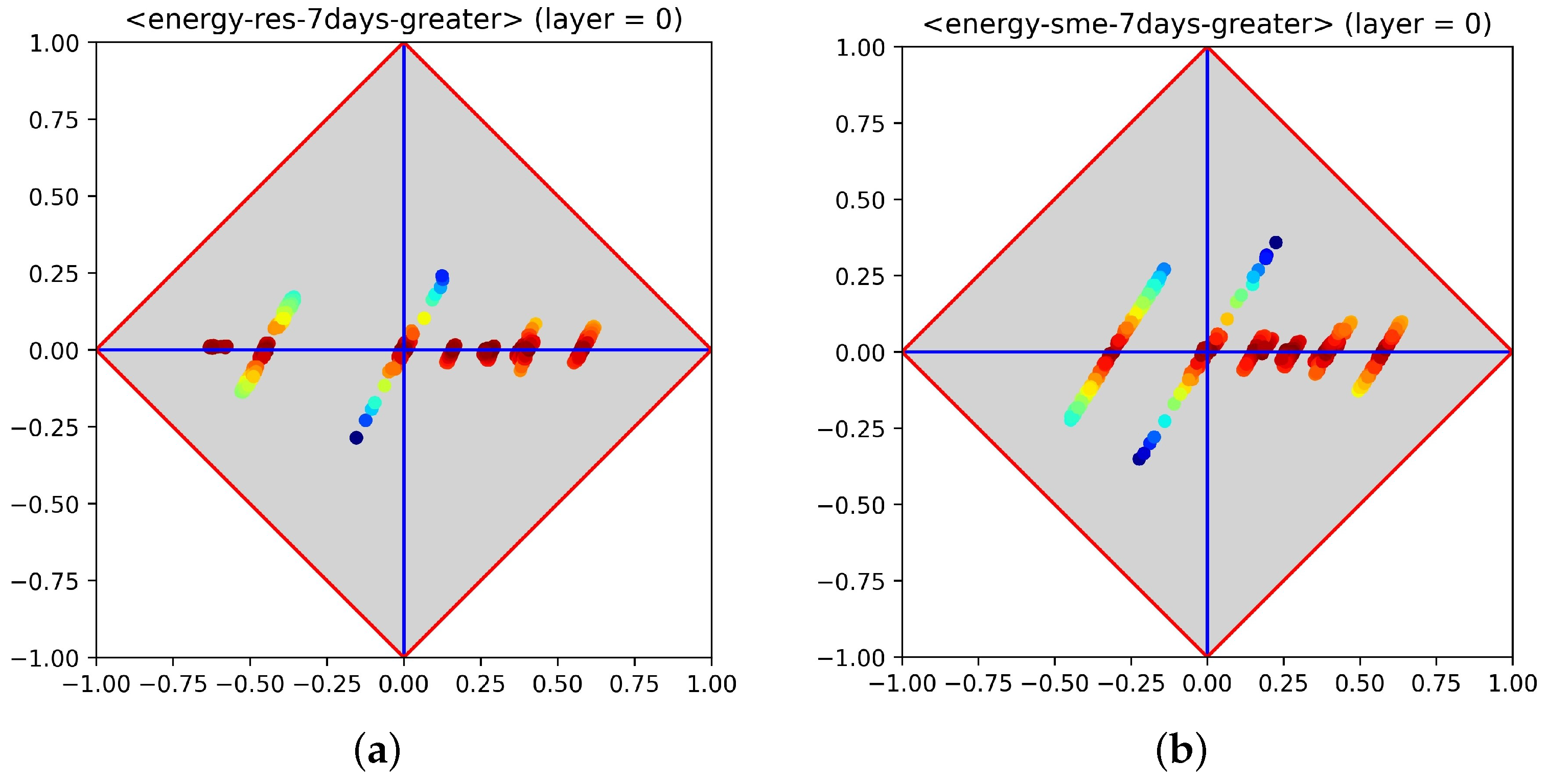
Let us recall that the underlying task consists of predicting the next-hour load, that the datasets used available for experiments were generated by applying 7-days windowing to the available raw data and that the shift from regression to classification was made by imposing a qualitative range on loads (i.e., lower, equal and greater). Since diagrams can only cope with binary problems, target labels were binarized according to the well-known “one-vs-rest” approach. As an example, Figure 3 shows the class signatures for residential and enterprise data for the label greater as positive category, whereas equal and lower (grouped together) represent the negative category. The reported diagrams provide an account of the importance that each single feature can have for the prediction. From a first glance, it is clear that both problems were apparently not easy to solve, as many features were located in proximity of the axis (recall that maximum entropy holds along this axis), whereas the remaining features appeared not far from it. Note that both diagrams highlight the presence of characteristic stripes. This fact can be explained by considering that the data used for experiments were derived by sliding a window over 7 days of recorded data, suggesting that the underlying process is quasi-stationary.
Summarizing, there was no clear cue on the existence of features with a significant impact on the classification. However, the training process might still be effective, due to the capability of MLPs to act as suboptimal feature combiners. To investigate this issue, the subsequent step was to train some MLP models, with the goal of checking whether they were able to perform generalisation on the given datasets. In particular, three models were trained on the dataset of residential customers (one for each target label, using a one-vs-rest approach) and the same was performed for enterprise customers.
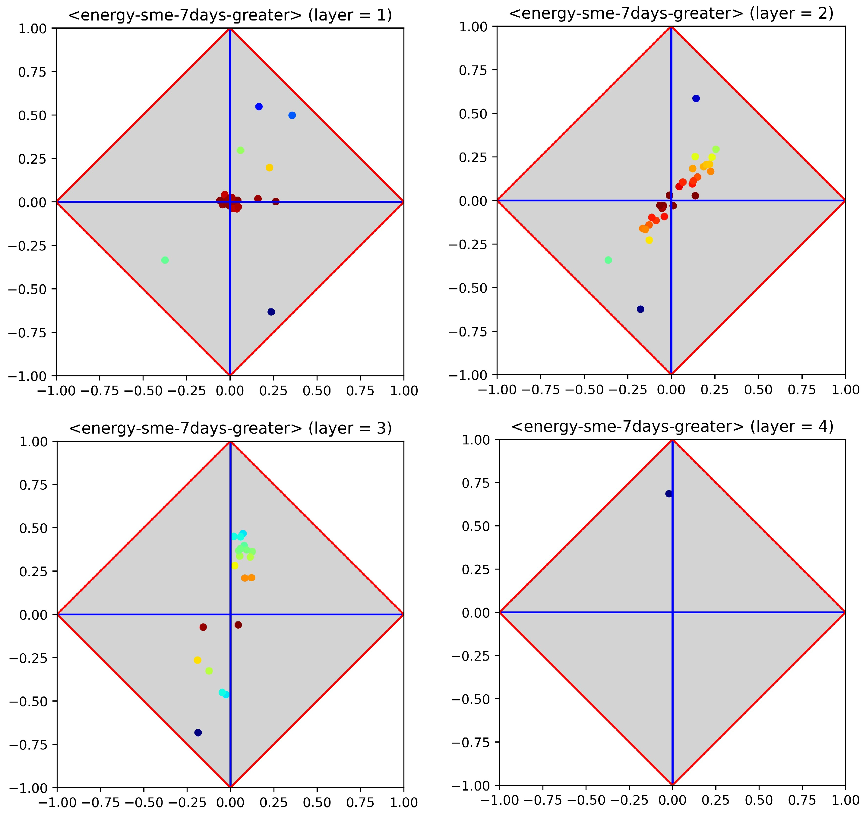
Figure 4 provides information on the encoding activity carried out by an MLP equipped with three hidden layers of 40, 30 and 20 neurons, which was trained on the dataset of residential customers, whereas Figure 5 reports the results of the training process carried out on the dataset of enterprise customers for the same problem. The focus was on electrical loads that were greater than those measured in the previous hour.
For both the MLPs dealing with residential and enterprise data, many neurons of the first hidden layer lay in proximity of the left or right corners. In fact, these MLPs reacted to the high number of features by putting some neurons in saturation, meaning that these neurons emitted the same value regardless of the input. Nevertheless, the signatures of the subsequent layers highlighted that the MLPs were able to cope with this issue. The last diagrams (bottom right, in both figures) report the performance of the MLPs after training (let us recall that, by definition, ; hence corresponds to an unbiased accuracy of ). Note that no significant changes were observed on the results while using alternative architectures, regardless of the number of hidden layers and of the number of neurons embedded therein. In particular, MLPs with between one and four hidden layers were repeatedly trained. Most of the changes in the number of neurons were experimented on the first hidden layer, varying from 40 to 200. Most likely, this lack of generalisation (observed on each test run) was due to the amount of input features. To investigate this issue, further experiments were carried out, as described in the next subsection.
3.2. Experiments on Datasets with Selected Features
Further experiments were made to assess whether the simplicity of the adopted encoding had triggered problems relating to the high number of features. The most straightforward FS strategy is dropping the features deemed less relevant after ranking them with a suitable heuristic function. In this research study, features were ranked according to their value—the lower the value, the less important the features. In particular, only 60 features out of 1848 were retained. In so doing, the threat due to the high number of features was removed, as about 97% of features were dropped.
Additionally, in this case, class signatures were calculated (on each dataset) for each target label. Figure 6 shows the signatures for residential and enterprise data using the label greater as positive category. In both cases, the signatures highlighted the presence of three separate clusters of overlapping features. This means that, given a cluster, all features that lay therein were expected to give the same performance if converted into a single-feature classifier. To check if FS was advantageous in terms of performance, further MLP models were trained, as performed with experiments designed using the full set of features. Figure 7 and Figure 8 provide information about the encoding activity performed by two MLPs equipped with three hidden layers of 40, 30 and 20 neurons and trained on the dataset of residential and enterprise customers. Again, the focus was on electrical loads greater than those measured in the previous hour and the last diagrams (bottom right, in both figures) report the performance of the MLPs after training.
In both cases, the first hidden layer highlighted that some neurons lay close to the centre of the diagram; hence, they could potentially be harmful to subsequent layers. However, the second and third layers illustrated that the MLPs were able to generalise despite the presence of these noisy neurons. In fact, as shown by the signature of the second hidden layers, the layer-wise strategy used to train the MLPs was able to properly handle this uncertainty by creating neurons that stood close to the upper or lower corners. The same pattern of generalisation was repeated in the signatures concerning the third hidden layer. After repeating the tests 10 times (using random sampling without replacement to generate training and test sets), again, no significant changes were observed in the results. Summarizing, there is evidence that the adopted FS algorithm used as preprocessing step helped the rise in generalisation.
Table 2 reports the experimental results obtained after training MLPs with PT on the two datasets. Each data instance ranged over a period of 7 days and each experiment was repeated 10 times. The average results obtained by training MLPs with the full set of 1848 features and with a selected set of 60 features point to the improvements obtained by means of FS. For residential customers, the increase was between 5% and 8% (average, 7%), whereas, for enterprise customers, it was between 2% and 5% (average, %). In fact, the differences in predicting the electrical loads of residential and enterprise customers were expected, as the latter—due to production patterns and routines—is typically more stable in terms of power demand.
4. Conclusions
The design of new monitoring systems for intelligent distribution networks, which allow the estimation of the state of the distribution system to be performed, requires both real-time measurements and pseudomeasurements to be processed. In this work, two datasets were analysed, which reported the power of the loads related to residential and enterprise customers. Using data generated by means of a 7-day time window, experiments were first carried out using the full set of 1848 features. The conjecture that the high number of features was possibly hampering the training process was further investigated by evaluating the performances obtained downstream of a feature selection step that allowed about of features to be dropped. In all the cases, the results obtained by training the MLP models with a selected set of features are better than those obtained with the full set of features. The analysis performed on the hidden layers of the trained MLP models also made clearer the dependence between the number of input features and the phenomenon of pattern formation during the training process. The approach adopted for the analysis has general applicability, as confirmed by its validity with very different types of loads (residential and SME) and different aggregation levels. This idea is strengthened by the fact that the behaviour of individual SM loads is clearly different over time and space and will change with the evolution of power grids and of the market, but aggregated loads are expected to have a more stable behaviour. Thus, the outcomes of the proposed analysis are subject to the variability in power consumption data, but we expect the methodology to be also valid for different scenarios.
The possibility of analysing the hidden layers of an MLP with diagrams opens several research scenarios that may contribute, in the near future, to an advancement of the state of the art. In particular, highlighting the presence of neurons in saturation at any hidden layer is a clear indicator that the number of neurons therein is still too high. Conversely, the occurrence of generalisation patterns inside an MLP after feature selection is a direct confirmation that the selection process has had a positive impact on the performance of the MLP at hand. The main research line for future work is guided by the considerations made above. In particular, proper pruning strategies will be devised and experimented, with the goal of removing useless neurons generated by the training process. A radical shift has also been planned for the PT algorithm. In fact, an implementation of it under TensorFlow (with Keras) will be released soon, giving users the possibility to select a number of training strategies according to the options made available by the Keras backend. Experiments with real-valued targets, framed within the applicative domain of electrical load forecasting, are also on the way, together with alternative feature selection strategies based on measures.
Author Contributions
Conceptualization, G.A. and P.A.P.; methodology and software, G.A.; validation, investigation, and data curation, G.A. and P.A.P.; writing—original draft preparation, G.A.; writing—review and editing, G.A. and P.A.P.; visualization, G.A. and P.A.P.; project administration, G.A.; funding acquisition, P.A.P. All authors have read and agreed to the published version of the manuscript.
Funding
This research was funded by “Fondazione di Sardegna”—research project IQSS (Information Quality aware and Secure Sensor networks for smart cities).
Institutional Review Board Statement
Not applicable.
Informed Consent Statement
Not applicable.
Data Availability Statement
The data used in this research, regarding the project “Electricity Smart-Metering Customer Behaviour Trials”, provided by the Commission for Regulation of Utilities (formerly Commission for Energy Regulation), can be accessed via the Irish Social Science Data Archive-www.ucd.ie/issda (accessed on 22 December 2021).
Conflicts of Interest
The authors declare no conflict of interest.
References
- Della Giustina, D.; Pau, M.; Pegoraro, P.A.; Ponci, F.; Sulis, S. Electrical distribution system state estimation: Measurement issues and challenges. IEEE Instrum. Meas. Mag. 2014, 17, 36–42. [Google Scholar] [CrossRef]
- Heydt, G.T. The Next Generation of Power Distribution Systems. IEEE Trans. Smart Grid 2010, 1, 225–235. [Google Scholar] [CrossRef]
- Wu, J.; He, Y.; Jenkins, N. A robust state estimator for medium voltage distribution networks. IEEE Trans. Power Syst. 2013, 28, 1008–1016. [Google Scholar] [CrossRef]
- Manitsas, E.; Singh, R.; Pal, B.C.; Strbac, G. Distribution system state estimation using an artificial neural network approach for pseudo measurement modelling. IEEE Trans. Power Syst. 2013, 27, 1888–1896. [Google Scholar] [CrossRef]
- Hayes, B.P.; Gruber, J.K.; Prodanovic, M. A Closed-Loop State Estimation Tool for MV Network Monitoring and Operation. IEEE Trans. Smart Grid 2015, 6, 2116–2125. [Google Scholar] [CrossRef]
- Carcangiu, S.; Fanni, A.; Pegoraro, P.A.; Sias, G.; Sulis, S. Forecasting-Aided Monitoring for the Distribution System State Estimation. Complexity 2020, 2020, 4281219:1–4281219:15. [Google Scholar] [CrossRef]
- El khantach, A.; Hamlich, M.; Belbounaguia, N.E. Short-term load forecasting using machine learning and periodicity decomposition. AIMS Energy 2019, 7, 382–394. [Google Scholar] [CrossRef]
- Huo, L.; Fan, X.; Xie, Y.; Yin, J. Short-Term Load Forecasting Based on the Method of Genetic Programming. In Proceedings of the International Conference on Mechatronics and Automation, Harbin, China, 5–8 August 2007; pp. 839–843. [Google Scholar] [CrossRef]
- Aprillia, H.; Yang, H.T.; Huang, C.M. Statistical Load Forecasting Using Optimal Quantile Regression Random Forest and Risk Assessment Index. IEEE Trans. Smart Grid 2021, 12, 1467–1480. [Google Scholar] [CrossRef]
- Hong, Y.; Zhou, Y.; Li, Q.; Xu, W.; Zheng, X. A Deep Learning Method for Short-Term Residential Load Forecasting in Smart Grid. IEEE Access 2020, 8, 55785–55797. [Google Scholar] [CrossRef]
- Chen, K.; Chen, K.; Wang, Q.; He, Z.; Hu, J.; He, J. Short-Term Load Forecasting With Deep Residual Networks. IEEE Trans. Smart Grid 2019, 10, 3943–3952. [Google Scholar] [CrossRef] [Green Version]
- Bashari, M.; Rahimi-Kian, A. Forecasting Electric Load by Aggregating Meteorological and History-based Deep Learning Modules. In Proceedings of the 2020 IEEE Power & Energy Society General Meeting (PESGM), Montreal, QC, Canada, 2–6 August 2020; pp. 1–5. [Google Scholar] [CrossRef]
- Wang, G.; Giannakis, G.B.; Chen, J.; Sun, J. Distribution system state estimation: An overview of recent developments. Front. Inf. Technol. Electron. Eng. 2019, 20, 4–17. [Google Scholar] [CrossRef]
- Hippert, H.S.; Pedreira, C.E.; Souza, R.C. Neural networks for short-term load forecasting: A review and evaluation. IEEE Trans. Power Syst. 2001, 16, 44–55. [Google Scholar] [CrossRef]
- Rana, M.; Koprinska, I.; Agelidis, V.G. Feature Selection for Electricity Load Prediction. In International Conference on Neural Information Processing, ICONIP (2); Huang, T., Zeng, Z., Li, C., Leung, C.S., Eds.; Springer: Berlin/Heidelberg, Germany, 2012; Volume 7664, pp. 526–534. [Google Scholar]
- Robnik-Šikonja, M.; Kononenko, I. Theoretical and Empirical Analysis of ReliefF and RReliefF. Mach. Learn. 2003, 53, 23–69. [Google Scholar] [CrossRef] [Green Version]
- Hall, M.A. Correlation-based Feature Selection for Discrete and Numeric Class Machine Learning. In ICML; Langley, P., Ed.; Morgan Kaufmann: Burlington, MA, USA, 2000; pp. 359–366. [Google Scholar]
- Gao, X.; Li, X.; Zhao, B.; Ji, W.; Jing, X.; He, Y. Short-Term Electricity Load Forecasting Model Based on EMD-GRU with Feature Selection. Energies 2019, 12, 1140. [Google Scholar] [CrossRef] [Green Version]
- Eseye, A.T.; Lehtonen, M.; Tukia, T.; Uimonen, S.; Millar, R.J. Machine Learning Based Integrated Feature Selection Approach for Improved Electricity Demand Forecasting in Decentralized Energy Systems. IEEE Access 2019, 7, 91463–91475. [Google Scholar] [CrossRef]
- Kim, W.; Han, Y.; Kim, K.J.; Song, K. Electricity load forecasting using advanced feature selection and optimal deep learning model for the variable refrigerant flow systems. Energy Rep. 2020, 6, 2604–2618. [Google Scholar] [CrossRef]
- Sankari, S.; Chinnappan, J. An improved short term load forecasting with ranker based feature selection technique. J. Intell. Fuzzy Syst. 2020, 39, 6783–6800. [Google Scholar]
- Armano, G. A Direct Measure of Discriminant and Characteristic Capability for Classifier Building and Assessment. Inf. Sci. 2015, 325, 466–483. [Google Scholar] [CrossRef]
- CER. Electricity Smart Metering Customer Behaviour Trials Findings Report (CER/11/080a); Commission for Energy Regulation: Dublin, Ireland, 2011. [Google Scholar]
- Met Eireann (Irish Meteorological Service). Available online: http://www.met.ie (accessed on 22 December 2021).
- Bradley, A. The use of the area under the ROC curve in the evaluation of machine learning algorithms. Pattern Recognit. 1997, 30, 1145–1159. [Google Scholar] [CrossRef] [Green Version]
- Woods, K.S.; Bowyer, K.W. Generating ROC Curves for Artificial Neural Networks. IEEE Trans. Med. Imaging 1997, 16, 329–337. [Google Scholar] [CrossRef]
- Armano, G.; Giuliani, A. A two-tiered 2d visual tool for assessing classifier performance. Inf. Sci. 2018, 463–464, 323–343. [Google Scholar] [CrossRef]
- Armano, G. Using phidelta diagrams to discover relevant patterns in multilayer perceptrons. Sci. Rep. 2020, 10, 21334. [Google Scholar] [CrossRef] [PubMed]
- Armano, G.; Giuliani, A.; Neumann, U.; Rothe, N.; Heider, D. Phi-Delta-Diagrams: Software Implementation of a Visual Tool for Assessing Classifier and Feature Performance. Mach. Learn. Knowl. Extr. 2019, 1, 121–137. [Google Scholar] [CrossRef] [Green Version]
Figure 1.
Histograms regarding the difference between hourly power demands, for residential and enterprise customers. (a) Residential customers. (b) Enterprise customers.
Figure 1.
Histograms regarding the difference between hourly power demands, for residential and enterprise customers. (a) Residential customers. (b) Enterprise customers.

Figure 2.
Semantics of diagrams, applied to classifier performance measures (a) or feature importance assessment (b). The axis is on the abscissa, while the axis is on the ordinate. (a) Semantics for classifiers. (b) Semantics for feature importance.
Figure 2.
Semantics of diagrams, applied to classifier performance measures (a) or feature importance assessment (b). The axis is on the abscissa, while the axis is on the ordinate. (a) Semantics for classifiers. (b) Semantics for feature importance.

Figure 3.
Class signatures of the datasets relating to residential loads (a) and enterprise loads (b). The reported signatures regard the greater-vs-rest binarization over the full set of features. (a) Loads of residential customers. (b) Loads of enterprise customers.
Figure 3.
Class signatures of the datasets relating to residential loads (a) and enterprise loads (b). The reported signatures regard the greater-vs-rest binarization over the full set of features. (a) Loads of residential customers. (b) Loads of enterprise customers.

Figure 4.
Hidden layers of an MLP trained on the dataset relating to residential customers (full set of features). The focus was on predicting whether the next-hour load would be greater than the previous one.
Figure 4.
Hidden layers of an MLP trained on the dataset relating to residential customers (full set of features). The focus was on predicting whether the next-hour load would be greater than the previous one.

Figure 5.
Hidden layers of an MLP trained on the dataset relating to enterprise customers (full set of features). The focus was on predicting whether the next-hour load would be greater than the previous one.
Figure 5.
Hidden layers of an MLP trained on the dataset relating to enterprise customers (full set of features). The focus was on predicting whether the next-hour load would be greater than the previous one.

Figure 6.
Class signatures of the datasets relating to residential loads (a) and enterprise loads (b). The reported signatures regard the greater-vs-rest binarization over a selected set of features (about 3% of the total number of features). (a) Loads of residential customers. (b) Loads of enterprise customers.

Figure 7.
Hidden layers of an MLP trained on the dataset relating to residential customers (full set of features). The focus was on predicting whether the next-hour load would be greater than the previous one.
Figure 7.
Hidden layers of an MLP trained on the dataset relating to residential customers (full set of features). The focus was on predicting whether the next-hour load would be greater than the previous one.

Figure 8.
Hidden layers of an MLP trained on the dataset relating to enterprise customers (full set of features). The focus was on predicting whether the next-hour load would be greater than the previous one.
Figure 8.
Hidden layers of an MLP trained on the dataset relating to enterprise customers (full set of features). The focus was on predicting whether the next-hour load would be greater than the previous one.


Table 1.
List of features that characterise the available data, for both residential and enterprise customers.
Table 1.
List of features that characterise the available data, for both residential and enterprise customers.
| Feature | Type | Explanation |
|---|---|---|
| DryBulb | Float | Temperature of dry bulb |
| WetBulb | Float | Temperature of wet bulb |
| DewPoint | Float | Dew point temperature |
| Humidity | Float | Air humidity |
| Hour | Float | Current hour |
| dayOfWeek | Integer | Current time day of the week |
| prevWeekSameHourLoad | Float | Previous week load (same hour) |
| prevDaySameHourLoad | Float | Previous day load (same hour) |
| prevHourLoad | Float | Previous hour load |
| prev24HrAveLoad | Float | Average load over the previous 24 h |
| isWorkingDay | Boolean | States whether it is a working day or not |
Table 2.
Average results obtained by repeatedly training MLPs on the datasets that stored information about hourly electrical loads, for both residential end enterprise customers.
Table 2.
Average results obtained by repeatedly training MLPs on the datasets that stored information about hourly electrical loads, for both residential end enterprise customers.
| Residential | Enterprise | ||||
|---|---|---|---|---|---|
| Specificity | Sensitivity | Specificity | Sensitivity | ||
| All features | lower-vs-rest | 0.71 | 0.71 | 0.76 | 0.80 |
| equal-vs-rest | 0.69 | 0.71 | 0.74 | 0.76 | |
| greater-vs-rest | 0.70 | 0.72 | 0.77 | 0.79 | |
| Selected features | lower-vs-rest | 0.76 | 0.78 | 0.79 | 0.82 |
| equal-vs-rest | 0.75 | 0.77 | 0.77 | 0.81 | |
| greater-vs-rest | 0.78 | 0.80 | 0.81 | 0.84 | |
Publisher’s Note: MDPI stays neutral with regard to jurisdictional claims in published maps and institutional affiliations. |
© 2022 by the authors. Licensee MDPI, Basel, Switzerland. This article is an open access article distributed under the terms and conditions of the Creative Commons Attribution (CC BY) license (https://creativecommons.org/licenses/by/4.0/).
Share and Cite
MDPI and ACS Style
Armano, G.; Pegoraro, P.A. Assessing Feature Importance for Short-Term Prediction of Electricity Demand in Medium-Voltage Loads. Energies 2022, 15, 549. https://0-doi-org.brum.beds.ac.uk/10.3390/en15020549
AMA Style
Armano G, Pegoraro PA. Assessing Feature Importance for Short-Term Prediction of Electricity Demand in Medium-Voltage Loads. Energies. 2022; 15(2):549. https://0-doi-org.brum.beds.ac.uk/10.3390/en15020549
Chicago/Turabian StyleArmano, Giuliano, and Paolo Attilio Pegoraro. 2022. "Assessing Feature Importance for Short-Term Prediction of Electricity Demand in Medium-Voltage Loads" Energies 15, no. 2: 549. https://0-doi-org.brum.beds.ac.uk/10.3390/en15020549
Note that from the first issue of 2016, this journal uses article numbers instead of page numbers. See further details here.