Integrated Structural Dependence and Stochastic Dependence for Opportunistic Maintenance of Wind Turbines by Considering Carbon Emissions

Abstract

Wind turbines have a wide range of applications as the main equipment for wind-power generation because of the rapid development of technology. It is very important to select a reasonable maintenance strategy to reduce the operation and maintenance costs of wind turbines. Traditional maintenance does not consider the environmental benefits. Thus, for the maintenance problems of wind turbines, an opportunistic maintenance strategy that considers structural correlations, random correlations, and carbon emissions is proposed. First, a Weibull distribution is used to describe the deterioration trend of wind turbine subsystems. The failure rates and reliability of wind turbines are described by the random correlations among all subsystems. Meanwhile, two improvement factors are introduced into the failure rate and carbon emission model to describe imperfect maintenance, including the working-age fallback factor and the failure rate increasing factor. Then, the total expected maintenance cost can be described as the objective function for the proposed opportunistic maintenance model, including the maintenance preparation cost, maintenance adjustment cost, shutdown loss cost, and operation cost. The maintenance preparation cost is related to the economic correlation, and the maintenance adjustment cost is described by using the maintenance probabilities under different maintenance activities. The shutdown loss cost is obtained by considering the structural correlation, and the operation cost is related to the energy consumption of wind turbines. Finally, a case study is provided to analyze the performance of the proposed model. The obtained optimal opportunistic maintenance duration can be used to interpret the structural correlation coefficient, random correlation coefficient, and sensitivity of carbon emissions. Compared with preventive maintenance, the proposed model provides better performance for the maintenance problems of wind turbines and can obtain relatively good solutions in a short computation time.

1. Introduction

With the rapid development of wind-power generation technology, wind turbines have a more comprehensive range of applications as the leading equipment for wind-power generation. However, wind turbines operate in harsh environments, such as in high temperatures, extreme cold, and high altitudes. Compared with other repairable equipment, their operation and maintenance costs are higher, accounting for more than 15% of the life-cycle cost. Thus, it is essential to select a reasonable maintenance strategy to formulate a scientific maintenance plan to reduce the operation and maintenance costs of wind turbines.

Currently, an opportunistic maintenance strategy can be applied to the maintenance of large and complex equipment, such as general aircraft, rail transit trains, and port handling systems [1,2,3]. For opportunistic maintenance (OM), when a system subsystem is shut down or preventive maintenance needs to be adopted, if other subsystems meet the predetermined maintenance conditions, the opportunity to execute preventive maintenance in advance is obtained. It can dynamically combine the subsystems for preventive maintenance based on the deterioration trend of subsystems to reduce the frequent shutdown of the system and the scheduling of maintenance resources. A wind turbine is also a large complex system, and there are three different correlation relationships among its subsystems, including economic correlations, random failure correlations, and structural correlations. Thomas provides the definition of correlation [4]. Economic correlation refers to the replacement or maintenance costs of several components being less than the sum of their individual replacement or maintenance costs. Random failure correlation means that the failure rate or operation state of other components will be affected to a certain extent when some components fail. Structural correlation implies that some components must be replaced or at least removed in order to replace or repair failed components. Thus, the correlation of subsystems is considered in comparison with traditional maintenance strategies for maintaining a single component. The opportunistic maintenance strategy can better meet the maintenance demands of wind turbines [5].

For the opportunistic maintenance strategy for wind turbines, to study the economic correlation of subsystems [6,7,8,9,10], some references assume that the subsystems are independent. In the actual operation of wind turbines, there is a coupling relationship between subsystems, and failure does not occur independently. Thus, the references further study the random failure correlation among subsystems. Li et al. used the copula function to describe a joint risk model to establish a double-layer optimization model for wind turbine preventive maintenance. The lower-level optimization model that considers the degree of risk of wind turbines related to failure effectively reduces the risk degree in the whole life cycle of wind turbines [11]. Yeter et al. considered the operation state of components in wind turbines. The proportional failure model was used to describe the deterioration process of components and established the state opportunistic maintenance model by setting the state maintenance threshold and opportunistic maintenance threshold [12]. Zhong et al. considered the failure correlation of wind turbines and used the affected degree to describe the impact on one subsystem generated by the failure of other subsystems. The affected degree was also used as the decision-making factor of the maintenance strategy. The results showed that considering the fault correlation can solve over-repair and under-repair problems to a certain extent [13]. The above research considers one or two kinds of wind-turbine subsystem correlations and fails to consider the structural correlation for an opportunistic maintenance strategy for wind turbines. Moreover, research on structural correlation is about mechanical engineering. The literature established the multi-component maintenance model that considers structural correlation from the perspectives of the disassembly sequence, the renewal method of the maintenance plan, and the importance of decision variables [14,15,16]. However, the research on the opportunistic maintenance strategies that consider structural correlation for wind-turbine maintenance is still in its infancy.

The extension of wind turbines’ operation time can reduce the preventive maintenance cost per unit, and the performance can also degrade. A poor operation is accompanied by increased energy consumption, intensified environmental damage, and increased enterprise operation cost. Thus, appropriate maintenance decisions can reduce operation costs and carbon emissions. Minne and Crittenden evaluated the impact of residential floor maintenance activities on the environment [17]. Giustozzi et al. proposed a road maintenance strategy with the optimization objectives of environmental impact, cost, and pavement performance [18]. Noland and Hanson used the life-cycle assessment method to assess the greenhouse gas emissions from road maintenance. The study found that the emissions from maintenance activities accounted for 10% of total emissions [19]. Sikos and Klemes studied the relationship between system reliability, maintainability, and environmental impact, and showed that system reliability and maintainability played important roles in the realization of cleaner production [20]. Liu et al. proposed a remanufacturing maintenance model to minimize the global warming potential based on reliability and replacement theory [21]. Chiara et al. established a regular preventive maintenance model, integrated the circular economy concept, selected the most suitable spare parts for maintenance activities from the perspective of sustainability, and proved the necessity of introducing sustainability considerations into routine maintenance procedures through described cases [22]. Jasiulewicz-Kaczmarek and Gola pointed out that the manufacturing industry was undergoing relevant changes because of the challenges brought by the sustainable economic development model. The maintenance function was also changing its role to better support value creation and expand its attention to environmental and social factors [23]. Hennequin and Ramirez Restrepo proposed a joint production and maintenance strategy model to minimize the impacts on the environment, inventory, and maintenance costs [24]. Afrinaldi et al. proposed a mathematical model to determine the optimal plan for preventive replacement of components and to minimize the economic and environmental impacts of the components [25]. Huang et al. integrated maintenance and energy saving into the same model, and introduced the opportunistic maintenance window mechanism [26]. Xia et al. proposed an oriented energy maintenance framework based on the energy saving windows [27]. The relevant work can be seen in

Table 1. The relevant work.

Articles	Wind Turbines	Correlations			Considerations
		Economic	Random	Structural
Song et al. [6]	√	√			Farm layout design
Ren et al. [7]	√	√			Carbon emissions
Li et al. [8]	√	√			Multiple-component age
Li et al. [9]	√	√			Maintenance intervals
Zhu et al. [10]	√	√			Logistic delay & weather condition
Li et al. [11]	√		√	√	Failure mode
Zhong et al. [13]	√	√			Reliability & cost
Zhou et al. [14]			√	√	Stochastic failures & disassembly sequence
Iung et al. [15]				√	Multi-dependent components
Wu et al. [16]				√	Component importance
Current study	√	√	√	√	Carbon emissions

. Most of the literature only evaluates the impact of maintenance activities on the environment in a specific context, and does not consider the impact of maintenance activities on failure rate and energy consumption, or the impact of recovery on the environment and cost rate.

To devise more accurate and practical maintenance strategies for wind turbines, this paper’s contribution is to propose an opportunistic maintenance (OM) model that considers economic correlations, random correlations, and structural correlations among wind-turbine subsystems and carbon emissions. Random correlation describes the failure rate and reliability of wind turbines among the subsystems. The improvement factor is introduced into the failure rate and carbon emission model to describe imperfect maintenance. Moreover, the operation energy consumption of wind turbines increases with performance degradation. This paper further considers the reduction effect of wind-turbine recovery on costs and emissions. The benefits of wind-turbine recovery and the emissions of maintenance activities can be introduced into the proposed model by adopting the dynamic failure rate function and carbon emission function. The total expected maintenance cost can then be described as the objective function for the proposed opportunistic maintenance model, including the maintenance preparation cost, maintenance adjustment cost, shutdown loss cost, and operation cost. The operation cost is related to the energy consumption of wind turbines. Finally, a case study is provided to analyze the performance of the proposed model. The obtained optimal opportunistic maintenance interval can be used to interpret the structural correlation coefficient, random correlation coefficient, and sensitivity of carbon emissions. Compared with preventive maintenance, the proposed model provides better performance with wind-turbine maintenance problems and can provide relatively good solutions in a short computation time.

2. The Notation and Problem Description

2.1. Notation

$\beta ,\alpha$: Weibull distribution parameters

${\chi }_{i,j}$: Random correlation coefficient

$\chi$: Random correlation coefficient matrix

$\lambda$: Structural correlation coefficient matrix

$C_{mm}$: Total minor maintenance cost

$C_{om}$: Total opportunistic maintenance cost

$C_{pm}$: Total preventive maintenance cost

$c_{i,mm}$: Minor maintenance cost of subsystem i

$c_{i,om}$: Opportunistic maintenance cost of subsystem i

$c_{i,pm}$: Preventive maintenance cost of subsystem i

$c_l$: Downtime loss per unit

$T$: Life cycle

$EC$: Total expected maintenance cost

$E{C}_F$: Total expected maintenance preparation cost

$E{C}_L$: Total expected downtime loss

$E{C}_M$: Total expected maintenance adjustment cost

$f_i\left(t\right)$: Probability density distribution function of subsystem i

$g_i\left(t_i^o,t\right)$: Opportunistic maintenance probability density function of subsystem i

$h_i\left(t\right)$: Probability density function of subsystem i

$p_i\left(m\right)$: Minor maintenance probability of subsystem i

$p_i\left(o\right)$: Opportunistic maintenance probability of subsystem i

$p_i\left(p\right)$: Preventive maintenance probability of subsystem i

$R_i\left(t\right)$: Reliability function

$t_i^o$: Opportunistic maintenance time threshold

$t_i^p$: Preventive maintenance time threshold

$t^d$: Downtime

$t^m$: Maintenance time

$t^{set}$: Maintenance preparation time

$w$: Opportunistic maintenance interval

2.2. Problem Description

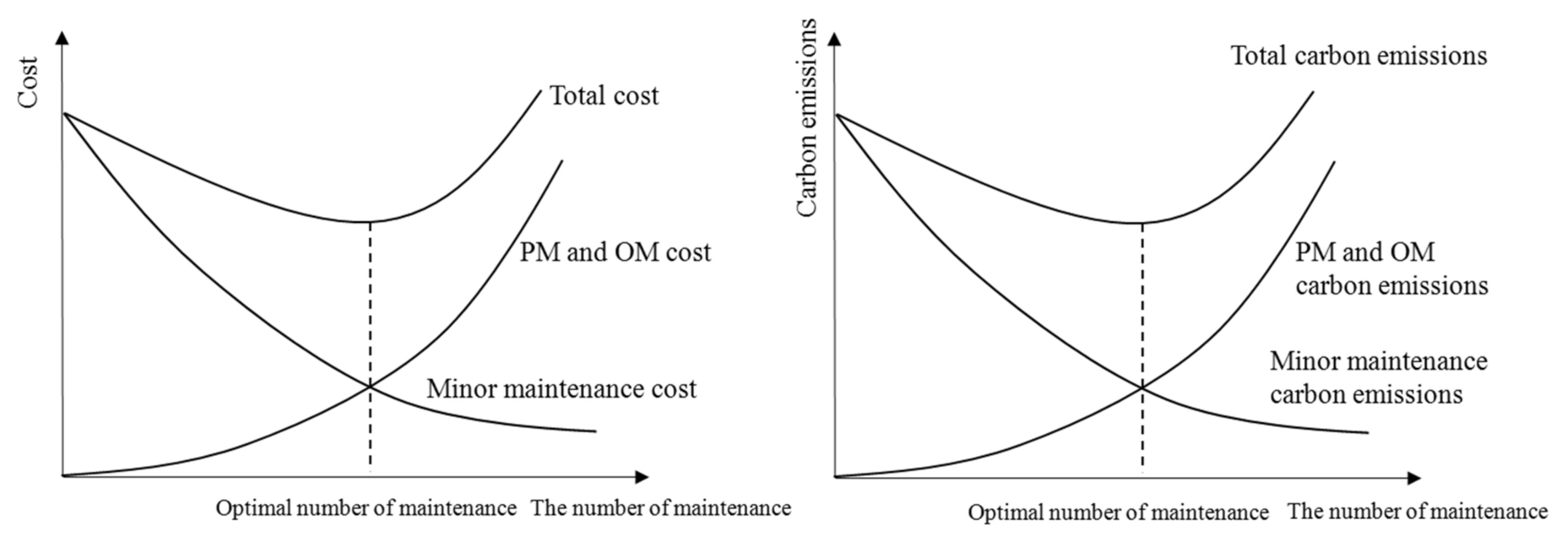
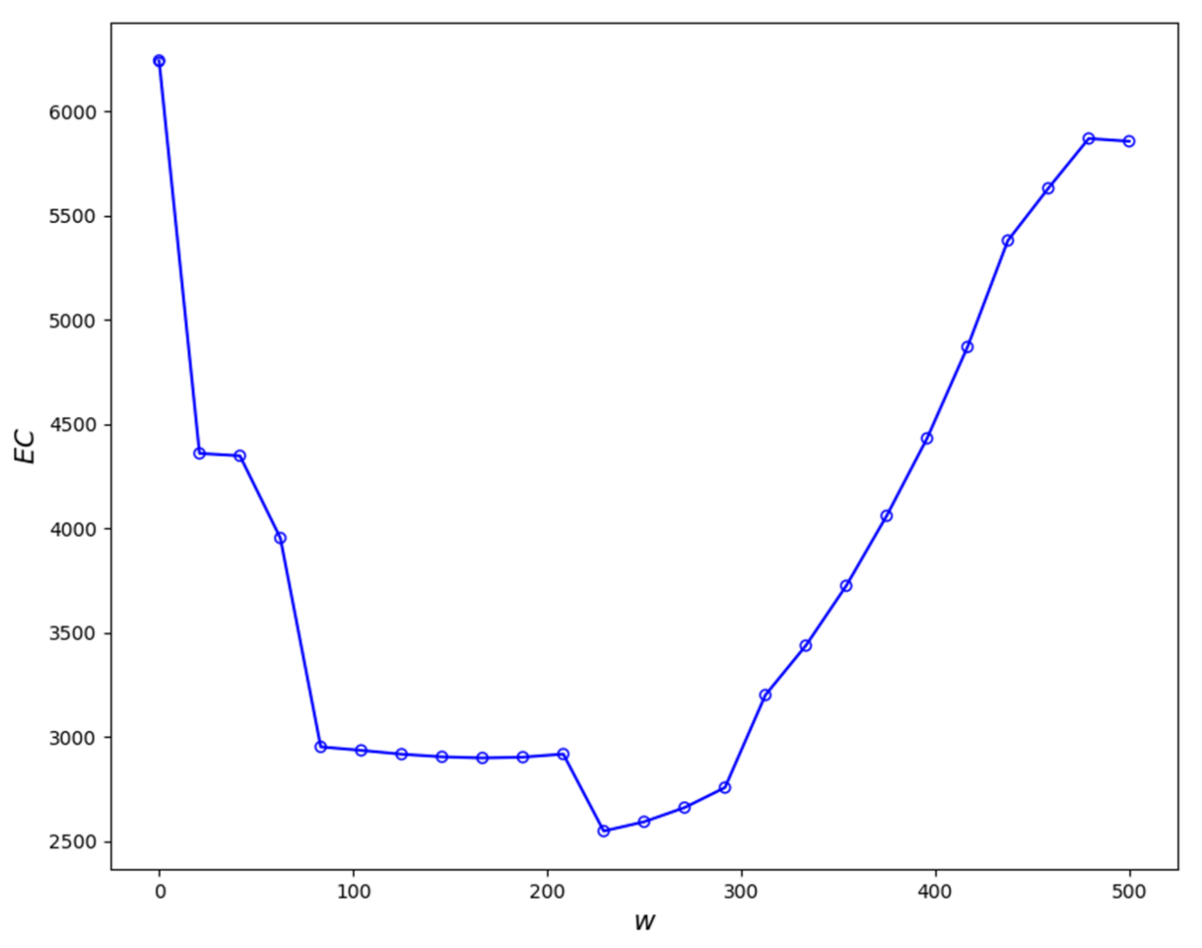
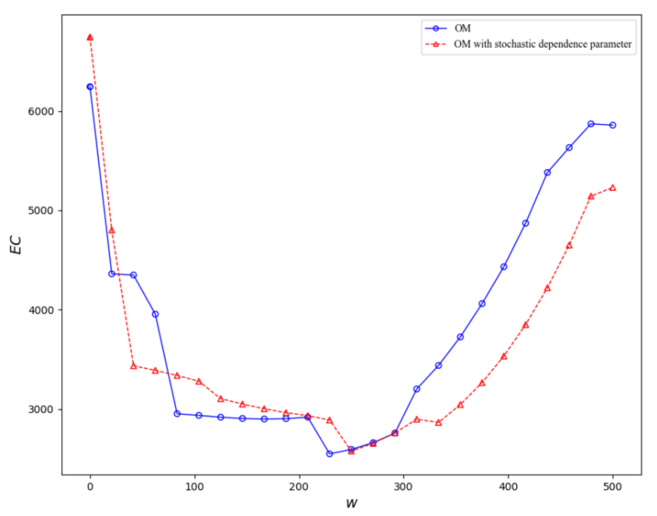
The extension of wind turbine operation time will reduce the preventive maintenance cost per unit, but the performance of the wind turbine will also degrade. For the life cycle of the wind turbine, the probability of unexpected failure becomes lower with an increase of the amount of preventive maintenance, and the amount of minor maintenance decreases. Most preventive maintenance (PM) strategies are undertaken, and the cost will increase. 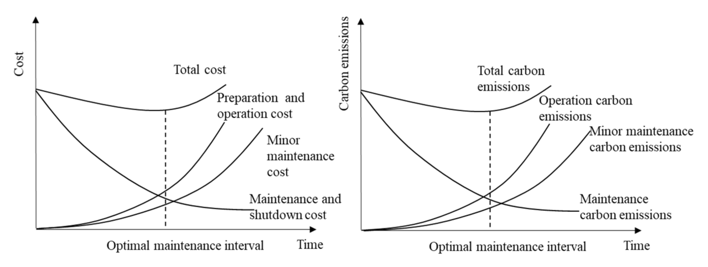The preventive maintenance cost is inversely proportional to the minor maintenance cost, as shown in Figure 1. The extension of wind turbine operation time will increase energy consumption, environmental damage, and operation cost, as shown in Figure 2.

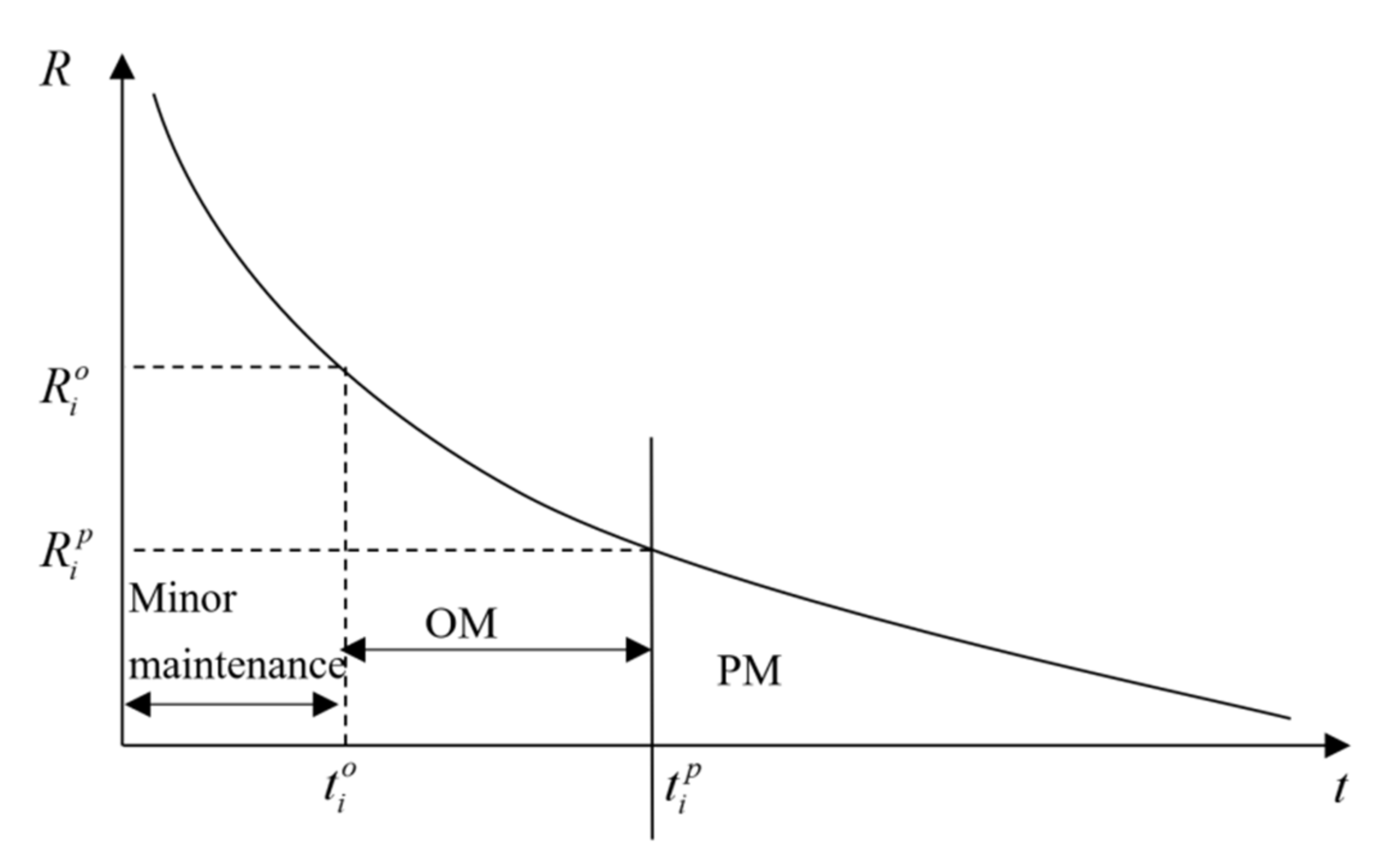
The wind turbine is taken as the research object, and the optimization goal is to minimize the expected total cost by considering the carbon emissions per unit. When a wind turbine has a sudden failure, it is necessary to carry out minor maintenance to ensure regular operation. Minor maintenance can only restore the function of the wind turbine to the state before the failure, without changing the failure rate and emission rate. Actually, wind turbine maintenance cannot affect a permanent repair as good as new, and the improvement factor is introduced to describe the impact of the maintenance actions on the wind turbine. The wind turbine consists of subsystems, and when preventive maintenance is applied to one subsystem, opportunistic maintenance can be applied to other subsystems.

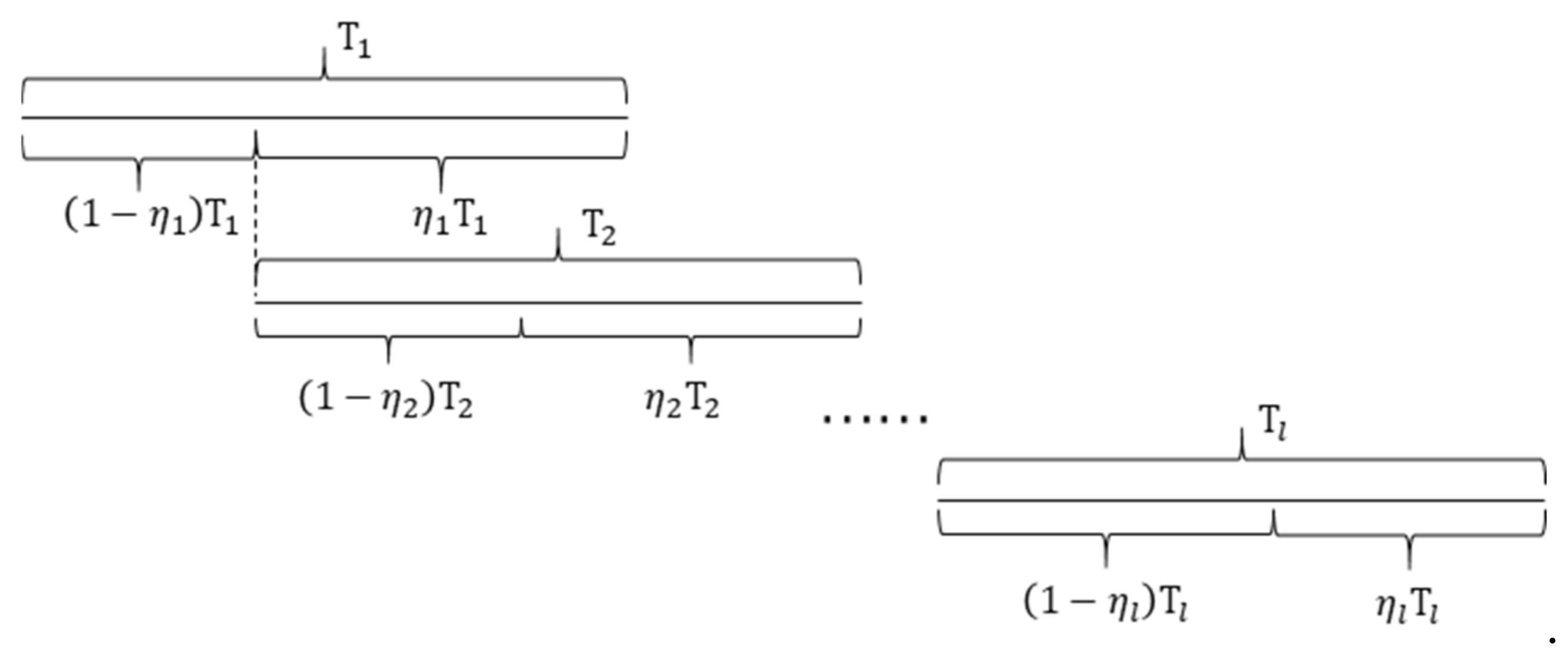
Let $t_i^p$ denote the preventive maintenance time threshold of wind turbine subsystem i, and $t_i^o$ the opportunistic maintenance time threshold. Thus, the opportunistic maintenance strategy of the wind turbine is shown in Figure 3.

Minor maintenance can be adopted for all failures of wind turbines before executing preventive maintenance and restore their operation state to that of before the fault. The instantaneous fault rate will not change. Preventive maintenance adopts the maintenance mode of replacement, which is regarded as a repair opportunity. If other subsystems meet the opportunistic maintenance conditions, they can be repaired simultaneously to the preventive maintenance of the subsystems when the wind turbine is shut down. Opportunistic maintenance can share maintenance resources during downtime and effectively reduce maintenance costs.

When the working age of subsystem i meets the condition $0<t<t_i^p$, if the subsystem i fails, minor repairs can be undertaken. This kind of maintenance aims to restore the state of the subsystem without changing its instantaneous failure rate. When the working age of subsystem i meets the preventive maintenance condition $t\ge t_i^p$, replacement can be undertaken to maintain subsystem i, and it can restore it to its initial health state.

Additionally, during the wind-turbine shutdown, other subsystems obtain maintenance opportunities. When the working age meets the condition $t_i^o<t<t_i^p$, the conditions of opportunistic maintenance are met, and all parts required for opportunistic maintenance during one shutdown are recorded in the set O, $O=\left\{1,2,\dots ,n\right\}$. Replacement can be undertaken to maintain subsystem i, and restore it to its initial health state.

3. The Model

3.1. Reliability Evolution

The traditional failure rate model usually takes the independence of component or system failure as the premise, and usually uses two parameters of a Weibull distribution to describe its degradation trend. The failure rate function and reliability function of subsystem i are respectively expressed as:

$$h_i^I\left(t\right)=\frac{{\beta }_i}{{\alpha }_i}{(\frac{t}{{\alpha }_i})}^{{\beta }_i-1}$$

(1)

$$R_i^I\left(t\right)=\exp \left[-{{\displaystyle \int }}_0^t{h}_i^I\left(t\right)dt\right]$$

(2)

where ${\beta }_i$ and ${\alpha }_i$ are the shape parameter and scale parameter of each subsystem, respectively, and ${\beta }_i>0,{\alpha }_i>0$.

During actual operation, there is a coupling relationship among subsystems, and their faults are not independent of each other. Murthy et al. proposed three types of random failure correlations [28,29]. Type I random failure correlation indicates that if a component in the system fails, it will lead to the failure of other internal components according to a certain probability. Type II random failure correlation indicates that one component failure in the system will affect other internal components’ failure rates to some extent. Type III is related to impact damage, specifically indicating that one component failure in the system will cause random damage to other internal components. The components will fail after the damage accumulates to a certain extent. In this paper, random correlation coefficient ${\chi }_{i,j}$ is introduced to describe the type II random failure correlation. Thus, the comprehensive instantaneous failure rate function of the subsystem can be expressed as:

$$h_i\left(t\right)=h_i^I\left(t\right)+{{\displaystyle \sum }}_j{\chi }_{i,j}{h}_j\left(t\right)$$

(3)

where, $i,j=1,2\dots n,i\ne j$, ${\chi }_{i,j}\in \left[0,1\right]$. ${\chi }_{i,j}=0$ indicates that there is no random failure correlation between two subsystems, and $h_i\left(t\right)=h_i^I\left(t\right)$. ${\chi }_{i,j}=1$ indicates that the two subsystems are completely related, and the failure of one subsystem will inevitably lead to the failure of the other subsystem.

Based on the failure transfer relationship among subsystems in a wind turbine, the failure transfer relationship diagram is shown as Figure 4. The matrix $\chi$ is used to record the quantized random correlation intensity coefficient ${\chi }_{i,j}$.

$$\chi =\left[\begin{array}{cccccccccccc}0& 0& 0& 0& 0& 0& 0& 0& 0& 0& 0& 0\\ {\chi }_{2,1}& 0& 0& 0& 0& 0& 0& {\chi }_{2,8}& 0& {\chi }_{2,10}& 0& 0\\ {\chi }_{3,1}& {\chi }_{3,2}& 0& {\chi }_{3,4}& {\chi }_{3,5}& {\chi }_{3,6}& 0& 0& 0& {\chi }_{3,10}& 0& 0\\ 0& 0& 0& 0& 0& 0& 0& {\chi }_{4,8}& 0& {\chi }_{4,10}& 0& 0\\ 0& 0& 0& 0& 0& 0& 0& {\chi }_{5,8}& 0& 0& 0& 0& \\ 0& 0& 0& 0& {\chi }_{6,5}& 0& 0& 0& 0& 0& 0& 0\\ 0& 0& 0& 0& 0& {\chi }_{7,6}& 0& {\chi }_{7,8}& 0& 0& 0& 0\\ 0& 0& 0& 0& 0& 0& 0& 0& {\chi }_{8,9}& 0& 0& 0\\ 0& 0& 0& 0& 0& 0& 0& 0& 0& 0& 0& 0\\ 0& 0& 0& 0& 0& 0& 0& {\chi }_{10,8}& 0& 0& 0& 0\\ 0& 0& 0& 0& 0& 0& 0& 0& 0& 0& 0& 0\\ 0& 0& 0& 0& 0& 0& 0& 0& 0& 0& 0& 0\end{array}\right]$$

Based on Equations (2) and (3), the reliability of the subsystem under the influence of comprehensive failure can be calculated. Thus, the comprehensive reliability function of the subsystem i is obtained.

$$R_i\left(t\right)=\exp \left[-{{\displaystyle \int }}_0^t{h}_i\left(t\right)dt\right]=R_i^I\left(t\right){{\displaystyle \prod }}_j{\left[R_j\left(t\right)\right]}^{{\chi }_{i,j}}$$

(4)

3.2. Improvement Factor

By adopting maintenance, the working age of a wind turbine will fall back to a previous stage. The fallback degree is related to maintenance cost and the amount of maintenance undertaken. The working age fallback factor is used to denote the effect of maintenance on the working age of wind turbines, and it can be obtained for subsystem i of a wind turbine.

$${\eta }_l={\left(a\frac{c_{i,om}}{c_{i,pm}}\right)}^{bl}$$

(5)

where, l represents l-th maintenance interval. $a$ is the cost adjustment coefficient, and it is used to adjust the opportunistic maintenance cost rate, $0\le a\le c_{i,pm}/c_{i,om}$. The opportunistic maintenance cost is higher, and the maintenance effect is better. $c_{i,om}$ is the opportunistic maintenance cost, $c_{i,pm}$ is the preventive replacement cost, and $b>1$ represents the time adjustment function. $0\le {\eta }_l\le 1$ and ${\eta }_l=0$ represent minor maintenance and ${\eta }_l=1$ shows preventive replacement. ${\eta }_l$ is larger or smaller, and it indicates whether the working age fallback after OM is more or less. When other parameters are determined, ${\eta }_l$ changes dynamically with the number of maintenance times. If the maintenance interval of a wind turbine is T, the effective working age of subsystem i after the first OM can be expressed as:

$$\begin{gathered} L_1^{-}=T_1 \\ {L}_1^{+}=t+\left(1-{\eta }_1\right)T_1 \end{gathered}$$

(6)

t is the time. In an l-th opportunistic maintenance interval, the value range of t is $t\in \left(0,T_l\right)$. By adopting OM, the working age falls back ${\eta }_1{T}_1$, and the effective working age becomes $t+\left(1-{\eta }_1\right)T_1$ after maintenance. It can then be deduced that the effective working age before and after the second OM can be expressed as:

$$\begin{gathered} L_2^{-}=L_1^{+}+T_2=t+\left(1-{\eta }_1\right)T_1+T_2 \\ {L}_2^{+}=t+\left(1-{\eta }_1\right)T_1+\left(1-{\eta }_2\right)T_2 \end{gathered}$$

(7)

The effective working age before and after $l-th$ $\left(l\ge 2\right)$ maintenance can be seen in Figure 5 and expressed as:

$$\begin{gathered} L_l^{-}=t+{{\displaystyle \sum }}_{j=1}^{l-1}\left(1-{\eta }_j\right)T_j+T_l \\ {L}_l^{+}=t+{\displaystyle \sum }_{j=1}^l\left(1-{\eta }_j\right)T_j \end{gathered}$$

(8)

where, $L_l^{-}$ represents the working age of subsystem i before $l-th$ maintenance and $L_l^{+}$ represents the working age of subsystem i after $l-th$ maintenance.

The maintenance will increase the working age of subsystem i, and change its failure rate curve. The failure rate increasing factor is used to express the impact of maintenance on the failure rate curve for subsystem i. The relationship between the failure rate functions before and after maintenance for subsystem i is as follows:

$$h_{l+1}\left(t\right)={\gamma }_l{h}_l\left(t\right)={{\displaystyle \prod }}_{j=1}^l{\gamma }_j{h}_1\left(t+{{\displaystyle \sum }}_{j=1}^l\left(1-{\eta }_j\right)T_j\right),t\in \left(0,T_{l+1}\right)$$

(9)

where, ${\gamma }_l$ is the change rate of the failure rate of subsystem i after adopting l-th maintenance, ${\gamma }_l\ge 1$. The failure rate curve changes under the action of different improvement factors, as shown in Figure 6. The red line describes the failure rate curve that considers the failure rate increasing factor. The blue line describes the failure rate curve that considers the working age fallback factor. The green line describes the failure rate curve that considers the working age fallback factor and the failure rate increasing factor.

Considering the reliability limit $R_{min}$ of subsystem i of a wind turbine, when the reliability is lower than $R_{min}$, maintenance is undertaken to restore the performance of subsystem i, and the reliability function can be obtained as follows:

$$\exp \left[-{{\displaystyle \int }}_0^{T_1}{h}_1\left(t\right)dt\right]=\exp \left[-{{\displaystyle \int }}_0^{T_2}{h}_2\left(t\right)dt\right]=\cdots =\exp \left[-{{\displaystyle \int }}_0^{T_N}{h}_N\left(t\right)dt\right]=R_{min}$$

(10)

Thus, the amount of minor maintenance for subsystem i in each maintenance interval is $-\ln R_{min}$, and each maintenance interval $\left[T_1,T_2,\cdots ,T_N\right]$ can be obtained by solving Equation (10).

3.3. Carbon Emission Model

The impact on the environment during the life cycle of a wind turbine mainly consists of carbon emissions from the energy consumption of using and recycling, and the recovery is considered to reduce carbon emissions. Carbon emissions during the life cycles of wind turbines are mainly generated by the energy consumed by operation and maintenance, construction/installation, and the decommissioning of wind turbines. Thus, the carbon emissions during the wind turbine life cycle can be expressed as follows:

$$GT=G_{use}X+\left(N+N_c\right)G_m+\left(1-{\delta }^{N-1}\right)G_p$$

(11)

where $G_{use}$ is the carbon emission generated by consuming an unit energy, $X$ is the total energy consumed during wind turbine operation, $N$ is the maintenance cycle, $N_c$ is the expected amount of minor maintenance undertaken, and $G_m$ is the carbon emission generated by undertaking one maintenance activity. Assuming that the carbon emissions generated by minor maintenance, OM and PM, are the same, $G_m$ is the same for each maintenance activity, ${\delta }^{N-1}$ is the recovery factor, and $G_p$ is the carbon emission generated by manufacturing a piece of a wind turbine.

$$X={{\displaystyle \int }}_0^{T_1}{x}_1\left(t\right)dt+{{\displaystyle \int }}_0^{T_2}{x}_2\left(t\right)dt+\cdots +{{\displaystyle \int }}_0^{T_N}{x}_N\left(t\right)dt={{\displaystyle \sum }}_{l=1}^N{{\displaystyle \int }}_0^{T_l}{x}_l\left(t\right)dt$$

(12)

$$N_c={{\displaystyle \int }}_0^{T_1}{\lambda }_1\left(t\right)dt+{{\displaystyle \int }}_0^{T_2}{\lambda }_2\left(t\right)dt+\cdots +{{\displaystyle \int }}_0^{T_N}{\lambda }_N\left(t\right)dt={{\displaystyle \sum }}_{l=1}^N{{\displaystyle \int }}_0^{T_l}{h}_l\left(t\right)dt$$

(13)

where, $x_l\left(t\right)$ is the energy consumption function of wind turbine operation. It can be obtained as follows:

$$x_1\left(t\right)=yt+z$$

(14)

where, y and z are the parameters of the wind turbine energy consumption function. The maintenance activities on wind turbines can restore performance and also change carbon emissions. Thus, the improvement factor can be introduced into the energy consumption function, and this is more in line with the actual situation. Before and after l-th maintenance, the relationship between energy consumption functions can be obtained as follows:

$$x_{l+1}\left(t\right)={{\displaystyle \prod }}_{j=1}^l{\gamma }_j{x}_1\left(t+{{\displaystyle \sum }}_{j=1}^l\left(1-{\eta }_j\right)T_j\right)={{\displaystyle \prod }}_{j=1}^l{\gamma }_j\left(y\left(t+{{\displaystyle \sum }}_{j=1}^l\left(1-{\eta }_j\right)T_j\right)+z\right)$$

(15)

The carbon emissions per unit during a wind turbine life cycle can be expressed as:

$$GWP=\frac{GT}{{{\displaystyle \sum }}_{l=1}^N{T}_l}=\frac{G_{use}X+G_m\left(N+N_c\right)+G_P\left(1-{\delta }^{N-1}\right)}{{{\displaystyle \sum }}_{l=1}^N{T}_l}=\frac{G_{use}\left({{\displaystyle \sum }}_{l=1}^N{{\displaystyle \int }}_0^{T_l}{x}_l\left(t\right)dt\right)+G_m\left(N+{{\displaystyle \sum }}_{l=1}^N{{\displaystyle \int }}_0^{T_l}{\lambda }_l\left(t\right)dt\right)+G_P\left(1-{\delta }^{N-1}\right)}{{{\displaystyle \sum }}_{l=1}^N{T}_l}$$

(16)

3.4. Expected Total Cost Model

Under the opportunistic maintenance strategy, the expected total maintenance cost of a wind turbine can be described as the objective function. For each maintenance cycle, the total maintenance cost is determined by the maintenance preparation cost $C_F$, maintenance operation cost TOC, maintenance adjustment cost $C_M$, and downtime cost $C_L$. The maintenance cost expectation is expressed as:

$$EC=E{C}_F+TOC+E{C}_M+E{C}_L$$

(17)

3.4.1. Maintenance Preparation Cost and Operation Cost

Before subsystem maintenance, maintenance personnel, vehicles, tower cranes, and other equipment are required to implement maintenance actions. Maintenance preparation costs mainly include labor services, vehicle transportation, and equipment rental fees. Assuming subsystem $i\in M$, M is the number of all the subsystems that require to be maintained in a maintenance activity. For the traditional maintenance strategy, the maintenance preparation cost depends on the total cost of the required maintenance subsystem, $E{C}_F={{\displaystyle \sum }}_{i\in M}{C}_i^0$. Under the opportunistic maintenance strategy, the economic correlation is considered when the subsystems are maintained. When multiple subsystems are maintained together, they share maintenance resources and allocate maintenance preparation costs. The expression of the maintenance preparation cost can be shown as follows:

$$E{C}_F=C_i^0$$

(18)

The wind-turbine performance degradation will increase its operation cost. The operation cost is related to its energy consumption. Let $C_e$ denote the consumption cost, and the total operation cost can be shown as follows:

$$TOC=C_{e}X=C_e{{\displaystyle \sum }}_{l=1}^N{{\displaystyle \int }}_0^{T_l}{x}_l\left(t\right)dt$$

(19)

3.4.2. Maintenance Adjustment Cost

In order to restore the subsystem to the normal operation state, different maintenance activities will produce different maintenance costs by implementing the maintenance strategy. These costs are collectively referred to as the maintenance adjustment cost, which include minor maintenance costs, preventive replacement costs, and opportunistic replacement costs. The maintenance probability is used to calculate the maintenance adjustment cost.

$p\left(m\right)$ indicates the probability for minor maintenance when the subsystem fails before preventive maintenance. $p\left(p\right)$ indicates the probability that subsystem k, which possibly executed PM, has no failure in interval $t\in \left(t_k^o,t_k^p\right)$, and subsystem i ($i\ne k$), which obtained OM, has good performance in this interval and does not need maintenance. $p\left(o\right)$ indicates the probability that subsystem k, which possibly executed PM in interval $t\in \left(t_k^o,t_k^p\right)$, is in good condition, but the subsystem r ($r\ne i\ne k$) experiences failure in this interval and needs to be replaced. The opportunistic maintenance time $t_i^o$ of subsystem i approximately obeys the exponential distribution, and its probability density function is:

$$g_i\left(t_i^o,t\right)=\frac{1}{{\alpha }_i}\exp \left[-\frac{t-t_i^o}{{\alpha }_i}\right]$$

(20)

The expectation function of the maintenance adjustment cost is obtained as follows:

$$E{C}_M=E\left(C_{mm}+C_{pm}+C_{om}\right)={{\displaystyle \sum }}_{i=1}^n\left[c_{i,mm}{p}_i\left(m\right)+c_{i,om}{p}_i\left(o\right)+c_{i,pm}{p}_i\left(p\right)\right]$$

(21)

The maintenance probability $p_i\left(m\right), p_i\left(p\right),p_i\left(o\right)$ can be shown as follows:

$$\begin{gathered} p_i\left(m\right)=\left\{\begin{array}{c}{{\displaystyle \int }}_0^{t_k^o}{f}_i\left(t\right)dt,i=k\hfill \\ {{\displaystyle \int }}_{t_k^o}^{t_k^p}{f}_k\left(t\right){\displaystyle {\displaystyle \prod }_i}\left[1-{{\displaystyle \int }}_{t_i^o}^{t_k^p}{g}_i\left(t_i^o,u\right)du\right]dt,i\in O\hfill \end{array}\right. \\ {p}_i\left(o\right)={{\displaystyle \int }}_{t_k^o}^{t_k^p}\left[\left(1-{{\displaystyle \int }}_{t_i^o}^t{f}_k\left(u\right)du\right)g_r\left(t_r^o,t\right){{\displaystyle \prod }}_{i\in O,i\ne r}\left(1-{{\displaystyle \int }}_{t_i^o}^{t_k^p}{g}_i\left(t_i^o,u\right)du\right)\right]dt \\ {p}_i\left(p\right)=\left[1-{{\displaystyle \int }}_{t_i^o}^{t_k^p}{f}_k\left(t\right)dt\right]{\displaystyle {\displaystyle \prod }_{i\in O}}\left[1-{{\displaystyle \int }}_{t_i^o}^{t_k^p}{g}_i\left(t_i^o,t\right)dt\right] \end{gathered}$$

(22)

3.4.3. Shutdown Loss Cost

The preventive replacement and opportunistic maintenance of a subsystem require the shutdown of a wind turbine to complete the maintenance activities. Thus, the wind turbine cannot generate power normally during this period, so the shutdown loss cost is calculated into the total maintenance cost. The downtime loss cost is equal to the loss cost per unit multiplied by the downtime, and can be obtained as follows:

$$C_L=c_l{t}^d=c_l\left(t^{set}+t^m\right)$$

(23)

For the maintenance process of wind turbines, the structural correlation is mainly demonstrated when multiple subsystems are maintained together, and one subsystem’s disassembly and installation process will affect other subsystems to a certain degree. The lost time of subsystem maintenance equals the summation of preventive maintenance $t_k^m$ and opportunistic maintenance $t_i^m$. The lost time of opportunistic maintenance is calculated by considering the structural correlation, and the subsystem that takes the longest time for opportunistic maintenance can be selected. The structure correlation matrix $\lambda$ is used to represent the strong relationships among the structures of subsystems. Thus, $t^m$ can be expressed as:

$$\begin{gathered} \lambda =\left[\begin{array}{cccc}{\lambda }_{1,1}& {\lambda }_{1,2}& \cdots & {\lambda }_{1,i}\\ {\lambda }_{2,1}& {\lambda }_{2,2}& \cdots & {\lambda }_{2,i}\\ ⋮& ⋮& \ddots & ⋮\\ {\lambda }_{i,1}& {\lambda }_{i,2}& \cdots & {\lambda }_{i,i}\end{array}\right] \\ {t}^m=t_k^m+{\lambda }_{k,i}\max \left\{t_i^m\right\},i\in O \end{gathered}$$

(24)

where structural correlation coefficient ${\lambda }_{i,j}\in \left[0,1\right),{\lambda }_{i,j}={\lambda }_{j,i}$. By combining with Equations (23) and (24), the expected shutdown loss cost can be obtained as follows:

$$E{C}_L=E\left(c_l{t}^d\right)=c_l\left[t^{set}+t_k^m{p}_k\left(p\right)+{\lambda }_{k,i}\max \left\{t_i^m\right\}{p}_i\left(o\right)\right]$$

(25)

Assuming that there are N maintenance cycles in the whole life cycle T, the expected total maintenance cost in the whole life cycle can be obtained as follows:

$$\begin{gathered} EC={\displaystyle \sum }_{l=1}^{N}E{C}^{\left(l\right)}={\displaystyle \sum }_{l=1}^N{\displaystyle \sum }_{i=1}^M\left[C_i^0+\left(c_{i,mm}{p}_i\left(m\right)+c_{i,om}{p}_i\left(o\right)+c_{i,pm}{p}_i\left(p\right)\right)+c_l{t}^d\right]+TOC \\ ={{\displaystyle \sum }}_{l=1}^N{{\displaystyle \sum }}_{i=1}^M\left[\begin{array}{c}{C}_i^0+\left(c_{k,mm}{{\displaystyle \int }}_0^{t_k^o}{f}_k\left(t\right)dt+c_{i,mm}{{\displaystyle \int }}_{t_k^o}^{t_k^p}{f}_k\left(t\right){{\displaystyle \prod }}_i\left[1-{{\displaystyle \int }}_{t_i^o}^{t_k^p}{g}_i\left(t_i^o,u\right)du\right]dt\right)\hfill \\ +c_{i,om}{{\displaystyle \int }}_{t_k^o}^{t_k^p}\left[\left(1-{{\displaystyle \int }}_{t_i^o}^t{f}_k\left(u\right)du\right)g_r\left(t_r^o,t\right){{\displaystyle \prod }}_{i\in O,i\ne r}\left(1-{{\displaystyle \int }}_{t_i^o}^{t_k^p}{g}_i\left(t_i^o,u\right)du\right)\right]dt\hfill \\ +c_{i,pm}\left[1-{{\displaystyle \int }}_{t_k^o}^{t_k^p}\left[f_k\left(t\right)\right]dt\right]{{\displaystyle \prod }}_{i\in O}\left[1-{{\displaystyle \int }}_{t_i^o}^{t_k^p}{g}_i\left(t\right)dt\right]\hfill \\ +c_l\left[t^{set}+t_k^m{p}_k\left(p\right)+{\lambda }_{k,i}\max \left\{t_i^m\right\}{p}_i\left(o\right)\right]\hfill \end{array}\right]+TOC \end{gathered}$$

(26)

4. The Procedure of Solving Model

In the opportunistic maintenance model, when the opportunistic maintenance threshold $t_i^o$ is being changed, subsystem $i\in O$ meeting the opportunistic maintenance conditions will change, directly affecting the maintenance plan of the next cycle, and dynamically changing the whole maintenance process and the total maintenance cost. It is assumed that the length of the opportunistic maintenance interval of each subsystem is the same, and this lets $w$ denote the length of the opportunistic maintenance interval, $t_i^o=t_i^o-w$. In $w\in \left[0,\min \left\{t_i^p\right\}\right]$, the total maintenance cost $EC$ under the opportunistic maintenance threshold is minimized by traversing $w$. $w^{*}$ is the optimal opportunistic maintenance duration and $t_i^{o*}=t_i^p-w^{*}$ is the optimal opportunistic maintenance threshold. 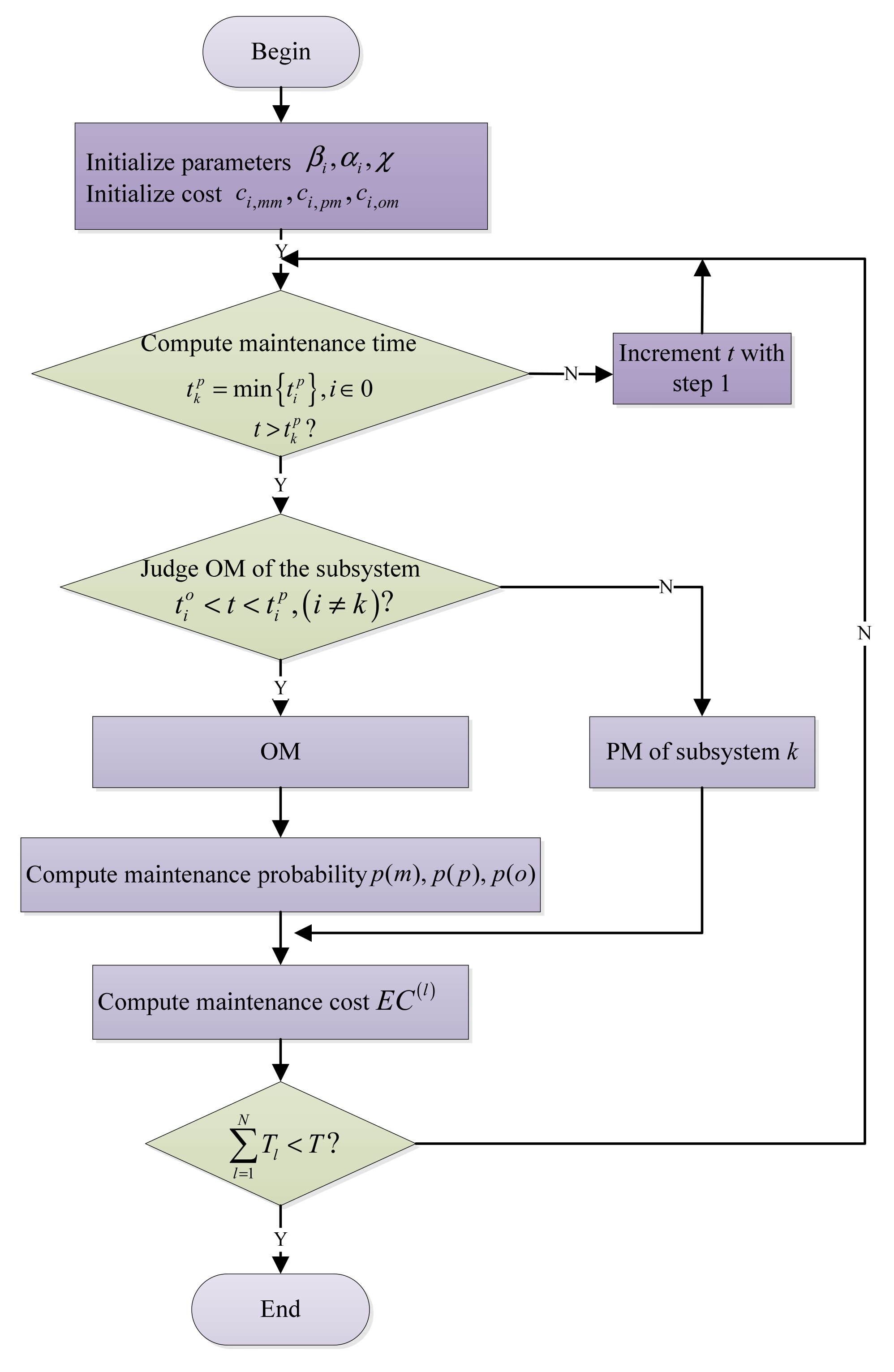Figure 7 is the solution flow chart, k describes the subsystem to possibly receive PM, and i $\left(j\ne k\right)$ describes the subsystem to possibly receive OM simultaneously. The specific calculation steps are as follows:

Step 1. Input the known condition, Weibull distribution parameters, failure correlation coefficient, and maintenance cost.

Step 2. Judge whether the running time t reaches the preventive maintenance threshold $t_k^p=\min \left\{t_i^p\right\}, i\in O$. If $t<t_k^p$, update the run time $t=t+1$ and cycle the step until the preventive maintenance conditions are met.

Step 3. For other subsystems $i\left(i\ne k\right)$ that have not experienced failure, calculate $t_i^o$ and judge whether the subsystem needs maintenance based on the value of w. If $t_i^o<t<t_i^p$, subsystem i meets the opportunistic maintenance conditions, and group maintenance is performed on subsystems i and k. If the opportunistic maintenance conditions are not met by i, subsystem k shall receive preventive maintenance separately. Calculate maintenance probability $p\left(m\right),p\left(p\right),p\left(o\right)$ and maintenance cost expectation $E{C}^{\left(l\right)}$ of the l-th maintenance cycle. Update $T_l=t_k^p+t^d$.

Step 4. If ${{\displaystyle \sum }}_{l=1}^N{T}_l<T$, return to Step2 for the next cycle of maintenance. Until ${{\displaystyle \sum }}_{l=1}^N{T}_l\ge T$. Exit the cycle.

Step 5. Calculate the expected total maintenance cost $EC$ in the whole life cycle, determine the optimal opportunistic maintenance interval $w^{*}$, and the optimal opportunistic maintenance threshold $t_i^{o*}$.

5. Case Study

5.1. Data Preparation

This paper selects the same type of wind turbine in a wind farm for case analysis. The key components of the subsystem are used to analyze the impeller system, spindle system, gearbox, and generator, numbered 1–4. The specified service life of such wind turbines is 15 years. The Weibull distribution parameters, single maintenance cost, and maintenance time of the subsystem are shown in

Table 2. Maintenance parameters.

$\mathbf{No}.\mathit{i}$	Subsystem	Weibull Distribution Parameters		Maintenance Cost (Unit: 10,000 yuan)					Maintenance Time (Unit: h)
		${\mathit{\alpha }}_{\mathit{i}}$	${\mathit{\beta }}_{\mathit{i}}$	${\mathit{C}}_0$	${\mathit{c}}_{\mathit{m}\mathit{m}}$	${\mathit{c}}_{\mathit{p}\mathit{m}}$	${\mathit{c}}_{\mathit{o}\mathit{m}}$	${\mathit{c}}_{\mathit{l}}$	${\mathit{t}}^{\mathit{s}\mathit{e}\mathit{t}}$	${\mathit{t}}_{\mathit{i}}^{\mathit{m}}$
1	Impeller system	3000	3	3.5	0.65	63.2	63.2	0.24	2	240
2	Spindle system	3750	2			65.8	65.8			480
3	Gearbox	2400	3			180.0	180.0			360
4	Generator	3300	2			75.7	75.7			168

.

The joint risk degree among components is used to describe the correlation degree of random failure among components. The random correlation coefficient matrix $\chi$ is obtained by combining the failure correlation coefficient and the wind turbine failure transmission diagram (Figure 4).

$$\chi =\left[\begin{array}{cccc}0& 0& 0& 0\\ 0.031& 0& 0& 0\\ 0.042& 0.13& 0& 0.11\\ 0& 0& 0& 0\end{array}\right]$$

(27)

Based on the reliability requirements for failure-free operation of wind turbines and referring to the reliability image of subsystems (see Figure 8), in Figure 8, the unit of values in the abscissa is a day. The preventive maintenance time threshold of the subsystem is obtained under this requirement (see

Table 3. Preventive maintenance reliability threshold and its corresponding time threshold.

$\mathbf{Subsystem}\mathbf{No}.\mathit{i}$	1	2	3	4
$R_i^p$	0.94	0.95	0.96	0.96
$t_i^p$(Unit: day)	823	536	619	529

).

5.2. Comparison of PM and OM

Compared with a preventive maintenance model based on the three-stage time delay theory proposed in the literature [30], opportunistic maintenance mainly considers the economic correlation among subsystems. The maintenance cost decreases with the reduction of downtime.

Table 4. Comparison of maintenance results between PM [30] and OM.

Cycle	PM [30]		$\mathbf{OM}(\mathit{w} = 220)$
	t (Unit: day)	$\mathbf{Subsystem}\mathit{i}$	t (Unit: day)	$\mathbf{PM}\mathbf{Subsystem}\mathit{k}$	$\mathbf{OM}\mathbf{Subsystem}\mathit{i}$
1	529	4	529	4	2
2	536	2	619	3	1
3	619	3	1058	4	2, 3
4	823	1	1442	1	2, 3, 4
5	1058	4	1971	4	2
6	1072	2	2061	3	1
7	1238	3	2500	4	2, 3
8	1587	4	2884	1	2, 3, 4
$⋮$	$⋮$	$⋮$	—	—	—
15	2476	3	5384	4	2, 3
$⋮$	$⋮$	$⋮$	—	—	—
34	5360	2	—	—	—

gives the maintenance results of wind turbines under two maintenance strategies: traditional preventive maintenance and opportunistic maintenance. Under the preventive maintenance strategy, the total number of wind turbine shutdowns in the whole life cycle is thirty-four. In the opportunistic maintenance strategy, the total number of wind turbine downtimes is fifteen, and the number of wind turbine downtimes is reduced by nineteen, accounting for about 55.88%.

Figure 9 shows the changing trend of total maintenance costs with increasing opportunistic maintenance interval $w$. In Figure 9, the unit of values in the abscissa is a day, and the unit of values in the ordinate is 10,000 yuan. For $w=0$, opportunistic maintenance is not considered. Thus, frequent downtime leads to high maintenance preparation costs, and the expected value of the total maintenance cost is $EC=6244.01$ (Unit: 10,000 yuan). After considering opportunistic maintenance, the probability of subsystems increases with the increase of $w$, and the cost of opportunistic maintenance increases continuously. Due to the reduction of downtime, the maintenance preparation cost and downtime loss cost are greatly reduced in opportunistic maintenance. For $w^{*}=220$ (unit: day), the optimal value of the objective function is 2547.98 (unit: 10,000 yuan). Finally, compared with not considering opportunistic maintenance, the expected total maintenance cost can be decreased by 3696.03 (unit: 10,000 yuan), accounting for about 59.19%.

5.3. OM Considering Structural Correlation and Random Correlation

For opportunistic maintenance, the impact of random correlation on wind turbine maintenance activities is considered. Type II random correlation accelerates the failure speed of subsystems to varying degrees. The preventive maintenance time threshold of a subsystem to meet the requirements of operation reliability will be affected by the random correlation coefficient and change.

Table 5. PM time threshold with the consideration of stochastic dependence.

$\mathbf{Subsystem}\mathbf{No}.\mathit{i}$	1	2	3	4
$t_i^p$(Unit: day)	823	530	514	529

shows the preventive maintenance time threshold calculated after considering the random correlation. Under the influence of subsystems 1, 2, and 4, subsystem 3 is 105 days ahead of that without considering the random correlation, becoming the subsystem that takes the lead in meeting the preventive maintenance reliability requirements, and the maintenance plan changes accordingly. Compared with the opportunistic maintenance strategy without considering random correlation, taking the maintenance plan when the length of opportunistic maintenance interval is 220 as an example (see

Table 6. Maintenance results under OM considering stochastic dependence ($w=220$).

Cycle	t (Unit: day)	PM Subsystem $\mathit{k}$	OM Subsystem $\mathit{i}$	Cycle	t (Unit: day)	PM Subsystem $\mathit{k}$	OM Subsystem $\mathit{i}$
1	514	3	2, 4	9	3229	1	3
2	823	1	3	10	3449	4	2
3	1043	4	2	11	3788	3	2, 4
4	1382	3	2, 4	12	4052	1	—
5	1664	1	--	13	4307	3	2, 4
6	1901	3	2, 4	14	4812	3	1, 2, 4
7	2406	3	2, 3, 4	15	5326	3	2, 4
8	2920	3	2, 4	—	—	—	—

), the expected total maintenance cost is 2888.51 (unit: 10,000 yuan). Due to the transformation of the maintenance action of subsystem 3 from OM to PM, the maintenance cost increases by 340.53.

Under OM by considering random correlation, when the opportunistic maintenance time interval is 240 (unit: day), the objective function obtains the optimal value 2576.13 (unit: 10,000 yuan) (see Figure 10). In Figure 10, the unit of values in the abscissa is a day, and the unit of values in the ordinate is 10,000 yuan. On this basis, the structural correlation among subsystems is further considered. For $w=240$ (unit: day), There are two types of maintenance classification: $M=\left\{3,2,4\right\}$, PM for subsystem 3, and OM for subsystems 2 and 4, and $M=\left\{1,2,3,4\right\}$, PM for subsystem 1, OM for subsystems 2, 3, and 4. Thus, when k executed PM equals 3 or 1, $\max \left\{t_i^m\right\}=t_2^m$. The structural correlation coefficients ${\lambda }_{3,2}$ and ${\lambda }_{1,2}$, and the impact on shutdown loss cost need to be considered.

${\lambda }_{3,2}$ and ${\lambda }_{1,2}$ are taken in sequence in units of 0.1 in the interval $\left[0,1\right]$ to calculate the shutdown loss cost. When the structural correlation coefficients are all 0, this means that only random correlation and economic correlation are considered. The shutdown loss cost is 993.24 (unit: 10,000 yuan). It can be seen from

Table 7. Downtime cost under different values of ${\lambda }_{3,2}$ and ${\lambda }_{1,2}$.

	${\mathit{\lambda }}_{1,2}$	0	0.1	0.2	0.3	0.4	0.5	0.6	0.7	0.8	0.9
${\mathit{\lambda }}_{3,2}$
0		993.24	985.30	977.36	969.41	961.47	953.53	945.59	937.65	929.70	921.76
0.1		986.83	978.88	970.94	963.00	955.06	947.12	939.17	931.23	923.29	915.35
0.2		980.41	972.47	964.53	956.59	948.65	940.70	932.76	924.82	916.88	908.94
0.3		974.00	966.06	958.12	950.17	942.23	934.29	926.35	918.41	910.46	902.52
0.4		967.59	959.64	951.70	943.76	935.82	927.88	919.93	911.99	904.05	896.11
0.5		961.17	953.23	945.29	937.35	929.40	921.46	913.52	905.58	897.64	889.69
0.6		954.76	946.82	938.87	930.93	922.99	915.05	907.11	899.17	891.22	883.28
0.7		948.34	940.40	932.46	924.52	916.58	908.64	900.69	892.75	884.81	876.87
0.8		941.93	933.99	926.05	918.11	910.16	902.22	894.28	886.34	878.4	870.45
0.9		935.52	927.58	919.63	911.69	903.75	895.81	887.87	879.92	871.98	864.04

that the shutdown loss cost decreases with the increase of the structural correlation coefficient. When ${\lambda }_{3,2}$ and ${\lambda }_{1,2}$ equal 0.9, the shutdown loss cost is 864.04 (unit: 10,000 yuan), which is reduced by 129.2 (unit: 10,000 yuan) compared with without considering the structural correlation. For ${\lambda }_{1,2}=0.9,{\lambda }_{3,2}=0$, the shutdown loss cost is reduced by 71.5 (unit: 10,000 yuan). For ${\lambda }_{1,2}=0,{\lambda }_{3,2}=0.9$, the shutdown loss cost is reduced by 57.7 (unit: 10,000 yuan). This shows that the structural correlation between subsystem 2 and subsystem 1 has a greater impact on the loss cost of a wind turbine.

5.4. Carbon Emission Analysis

The optimization results of the wind turbine carbon emission model indicates that the number of PM reaches 11, and the objective function value of the carbon emission model is the smallest and is $GWP=4015.7{\mathrm{g}\mathrm{CO}}_2-\mathrm{eq}$. Economic benefit is an essential factor that enterprises must consider. Under the comprehensive consideration of environmental and economic benefits, the best amount of preventive maintenance is optimal, and the goal involving carbon emissions is relatively good.

5.5. Sensitivity Analysis

This paper mainly analyzes the sensitivity of three parameters: carbon emission $G_{use}$ generated by wind turbine consumption per unit energy, carbon emission $G_m$ generated by wind turbine maintenance activities, and carbon emission $G_p$ generated by manufacturing one wind turbine.

(1) $G_{use}$. When $G_{use}$ is being changed, the carbon emission per unit operation of a wind turbine will also change, as will the optimal solution of the wind turbine carbon emission model. The changing trend is shown in Figure 11.

In Figure 11, the abscissa represents maintenance cycle N (i.e., the total amount of wind turbine downtime). The top line (green line) is $G_{use}=3195{\mathrm{gCO}}_2-\mathrm{eq}$, and the optimal $N^{*}=10$. The middle line (black line) is $G_{use}=2695{\mathrm{gCO}}_2-\mathrm{eq}$, and $N^{*}=11$. The bottom line (red line) is $G_{use}=1695{\mathrm{gCO}}_2-\mathrm{eq}$, and $N^{*}=14$. When the value of $G_{use}$ becomes larger (smaller), it means that the carbon emissions per unit of energy consumed by a wind turbine become larger (smaller), which will release more (less) greenhouse gas pollution into the environment during its operation. Thus, for a single carbon emission model, it is necessary to reduce (increase) the amount of preventive maintenance. Considering the cost rate comprehensively, when the value of $G_{use}$ becomes smaller, the value of the optimal solution of preventive maintenance times is more sensitive to the change. When the value of $G_{use}$ becomes larger, the value change of the optimal solution of preventive maintenance times is not sensitive.

(2) $G_m$. When $G_m$ is being changed, the change of wind turbine carbon emissions per unit operation is shown in Figure 12.

In Figure 12, the top line (green line) is $G_m=6450{\mathrm{gCO}}_2-\mathrm{eq}$, and $N^{*}=11$. The middle line (black line) is $G_{use}=\mathrm{11,450}{\mathrm{gCO}}_2-\mathrm{eq}$, and $N^{*}=11$. The bottom line (red line) is $G_{use}=1\mathrm{6,450}{\mathrm{gCO}}_2-\mathrm{eq}$, and $N^{*}=11$. It can be seen that when $G_m$ is being changed, the change of the optimal solution of the carbon emission model and the optimization decision model is not sensitive, but the carbon emission per unit operation is changed.

(3) $G_p$. When $G_p$ is being changed, the carbon emission per unit operation of a wind turbine will also change, and the optimal solution of the wind turbine carbon emission model will also change. The changing trend is shown in Figure 13.

From top to bottom, the first line (pink line) is $G_p=1{.6\times 10}^8{\mathrm{gCO}}_2-\mathrm{eq},N^{*}=16$, the second line (green line) is $G_p=9\times {10}^7{\mathrm{gCO}}_2-\mathrm{eq},N^{*}=12$, the third line (black line) is $G_p=8\times {10}^7{\mathrm{gCO}}_2-\mathrm{eq},N_g^{*}=11$, and the fourth line (red line) is $G_p=7\times {10}^7{\mathrm{gCO}}_2-\mathrm{eq},N^{*}=10$. When the value of $G_p$ becomes larger (smaller), it means that the carbon emissions generated by manufacturing one wind turbine become larger (smaller). For a single carbon emission model, it is necessary to increase (reduce) the amount of preventive maintenance to reduce the carbon emission per unit operation in the whole life cycle of a wind turbine. Considering the cost rate comprehensively, when the value of $G_p$ becomes larger, the value of the optimal solution of the preventive maintenance times is more sensitive. When the value of $G_p$ becomes smaller, the value of the optimal preventive maintenance times is not sensitive.

6. Conclusions

This paper mainly studies the opportunistic maintenance strategy of wind turbines. The economic correlation, random correlation, and structural correlation among subsystems and carbon emissions can be considered in the proposed maintenance model. The stochastic correlation coefficient matrix is constructed by a failure chain to describe the reliability of the subsystems, and the structural correlation coefficient is used to describe the downtime loss cost in order to present the opportunistic maintenance model. Moreover, the operation energy consumption of wind turbines increases with their performance degradation. The environmental benefits are combined in the maintenance model of wind turbines. The working age fallback factor and failure rate increasing factor are introduced to establish the carbon emission model and the total expected cost model. This paper further considers the reduction effect of wind turbines recovery on cost and emission. The benefits of wind turbines can introduce recovery and emissions of maintenance activities into the proposed model by adopting the dynamic failure rate function and carbon emission function. The total expected maintenance cost could be described as the objective function for the proposed opportunistic maintenance model, including maintenance preparation cost, maintenance adjustment cost, shutdown loss cost, and operation cost. The operation cost is related to the energy consumption of wind turbines. Finally, a case study is provided to analyze the performance of the proposed model. Compared with preventive maintenance, the proposed model demonstrates better performance on wind turbines maintenance problems and can obtain a relatively good solution in a short computation time. The method proposed in this paper provides certain significance for guiding the selection of a wind turbine maintenance strategy.

The proposed model does not consider the complex external operation environment and external impacts. Thus, the joint optimization model between the carbon emission model and condition-based maintenance that considers the external operation environment and effect needs to be developed in the future.

References

1. Gorbunov, V.; Kuznetsov, S.; Savvina, A.; Poleshkina, I. Methodological aspects of avionics reliability at low temperatures during aircraft operation in the Far North and the Arctic. Transp. Res. Procedia 2021, 57, 220–229. [Google Scholar] [CrossRef]
2. Lin, B.; Wu, J.; Lin, R.; Wang, J.; Wang, H.; Zhang, X. Optimization of high-level preventive maintenance scheduling for high-speed trains. Reliab. Eng. Syst. Saf. 2019, 183, 261–275. [Google Scholar] [CrossRef]
3. Appoh, F.; Yunusa-Kaltungo, A.; Sinha, J.K. Hybrid adaptive model to optimise components replacement strategy, a case study of railway brake blocks failure analysis. Eng. Fail. Anal. 2021, 127, 105539. [Google Scholar] [CrossRef]
4. Thomas, L.C. A survey of maintenance and replacement models for maintainability and reliability of multi-item systems. Reliab. Eng. 1986, 16, 297–309. [Google Scholar] [CrossRef]
5. Allal, A.; Sahnoun, M.; Adjoudj, R.; Benslimane, S.; Mazar, M. Multi-agent based simulation-optimization of maintenance routing in offshore wind farms. Comput. Ind. Eng. 2021, 157, 107342. [Google Scholar] [CrossRef]
6. Song, S.; Li, Q.; Felder, F.A.; Wang, H.; Coit, D.W. Integrated optimization of offshore wind farm layout design and turbine opportunistic condition-based maintenance. Comput. Ind. Eng. 2018, 120, 288–297. [Google Scholar] [CrossRef]
7. Ren, Z.; Verma, A.S.; Li, Y.; Teuwen, J.J.; Jiang, Z. Offshore wind turbine operations and maintenance, a state-of-the-art review. Renew. Sustain. Energy Rev. 2021, 144, 110886. [Google Scholar] [CrossRef]
8. Li, M.; Jiang, X.; Negenborn, R.R. Opportunistic maintenance for offshore wind farms with multiple-component age-based preventive dispatch. Ocean Eng. 2021, 231, 109062. [Google Scholar] [CrossRef]
9. Li, M.X.; Wang, M.; Kang, J.C.; Sun, L.P.; Jin, P. An opportunistic maintenance strategy for offshore wind turbine system considering optimal maintenance intervals of subsystems. Ocean Eng. 2020, 216, 108067. [Google Scholar] [CrossRef]
10. Zhu, W.J.; Castanier, B.; Bettayeb, B. A dynamic programming-based maintenance model of offshore wind turbine considering logistic delay and weather condition. Reliab. Eng. Syst. Saf. 2019, 190, 106512. [Google Scholar] [CrossRef]
11. Li, H.; Diaz, H.; Soares, C.G. A developed failure mode and effect analysis for floating offshore wind turbine support structures. Renew. Energy 2021, 164, 133–145. [Google Scholar] [CrossRef]
12. Yeter, B.; Garbatov, Y.; Soares, C.G. Life-extension classification of offshore wind assets using unsupervised machine learning. Reliab. Eng. Syst. Saf. 2022, 219, 108229. [Google Scholar] [CrossRef]
13. Zhong, S.; Pantelous, A.A.; Goh, M.; Zhou, J. A reliability-and-cost-based fuzzy approach to optimize preventive maintenance scheduling for offshore wind farms. Mech. Syst. Signal Processing 2019, 124, 643–663. [Google Scholar] [CrossRef] [Green Version]
14. Zhou, X.; Huang, K.; Xi, L.; Lee, J. Preventive maintenance modeling for multi-component systems with considering stochastic failures and disassembly sequence. Reliab. Eng. Syst. Saf. 2015, 142, 231–237. [Google Scholar] [CrossRef]
15. Iung, B.; Do, P.; Levrat, E.; Voisin, A. Opportunistic maintenance based on multi-dependent components of manufacturing system. CIRP Ann. 2016, 65, 401–404. [Google Scholar] [CrossRef]
16. Wu, S.; Chen, Y.; Wu, Q.; Wang, Z. Linking component importance to optimisation of preventive maintenance policy. Reliab. Eng. Syst. Saf. 2015, 146, 26–32. [Google Scholar] [CrossRef] [Green Version]
17. Minne, E.; Crittenden, J.C. Impact of maintenance on life cycle impact and cost assessment for residential flooring options. Int. J. Life Cycle Assess. 2015, 20, 36–45. [Google Scholar] [CrossRef]
18. Giustozzi, F.; Crispino, M.; Flintsch, G. Multi-attribute life cycle assessment of preventive maintenance treatments on road pavements for achieving environmental sustainability. Int. J. Life Cycle Assess. 2012, 17, 409–419. [Google Scholar] [CrossRef]
19. Noland, R.B.; Hanson, C.S. Life-cycle greenhouse gas emissions associated with a highway reconstruction, a New Jersey case study. J. Clean. Prod. 2015, 107, 731–740. [Google Scholar] [CrossRef]
20. Sikos, L.; Klemeš, J. RAMS contribution to efficient waste minimisation and management. J. Clean. Prod. 2009, 17, 932–939. [Google Scholar] [CrossRef]
21. Liu, Z.-C.; Afrinaldi, F.; Zhang, H.-C.; Jiang, Q. Exploring optimal timing for remanufacturing based on replacement theory. CIRP Ann.-Manuf. Technol. 2016, 65, 447–450. [Google Scholar] [CrossRef]
22. Franciosi, C.; Lambiase, A.; Miranda, S. Sustainable maintenance, a periodic preventive maintenance model with sustainable spare parts management. IFAC Pap. 2017, 50, 13692–13697. [Google Scholar] [CrossRef]
23. Jasiulewicz-Kaczmarek, M.; Gola, A. Maintenance 4.0 technologies for sustainable manufacturing-an overview. IFAC Pap. 2019, 52, 91–96. [Google Scholar] [CrossRef]
24. Hennequin, S.; Restrepo, L.M.R. Fuzzy model of a joint maintenance and production control under sustainability constraints. IFAC Pap. 2016, 49, 1216–1221. [Google Scholar] [CrossRef]
25. Afrinaldi, F.; Taufik; Tasman, A.M.; Zhang, H.-C.; Hasan, A. Minimizing economic and environmental impacts through an optimal preventive replacement schedule, model and application. J. Clean. Prod. 2017, 143, 882–893. [Google Scholar] [CrossRef]
26. Huang, J.; Chang, Q.; Arinez, J.; Xiao, G.X. A maintenance and energy saving joint control scheme for sustainable manufacturing systems. Procedia CIRP 2019, 80, 263–268. [Google Scholar] [CrossRef]
27. Xia, T.; Xi, L.; Zhou, X.; Du, S. Modeling and optimizing maintenance schedule for energy systems subject to degradation. Comput. Ind. Eng. 2012, 63, 607–614. [Google Scholar] [CrossRef]
28. Murthy, D.N.P.; Nguyen, D.G. Study of two-component system with failure interactions. Nav. Res. Logist. Q. 1985, 32, 239–247. [Google Scholar] [CrossRef]
29. Nakagawa, T.; Murthy, D.N.P. Optimal replacement policies for a two-unit system with failure interactions. Rairo Oper. Res. 1993, 27, 427–438. [Google Scholar] [CrossRef] [Green Version]
30. Lv, X.; Liu, Q.; Li, Z.; Dong, Y.; Xia, T.; Chen, X. A New Maintenance Optimization Model Based on Three-Stage Time Delay for Series Intelligent System with Intermediate Buffer. Shock. Vib. 2021, 2021, 6694896. [Google Scholar] [CrossRef]
Figure 1. Cost and carbon emission change with the amount of maintenance.
Energies 15 00625 g001
Figure 2. Cost and carbon emission change with the interval of maintenance.
Energies 15 00625 g002
Figure 3. Opportunistic maintenance strategies of wind turbines.
Energies 15 00625 g003
Figure 4. Fault transmission diagram of wind turbines.
Energies 15 00625 g004
Figure 5. Changes of effective working age of subsystem i before and after maintenance.
Energies 15 00625 g005
Figure 6. Change of failure rate curve before and after maintenance.
Energies 15 00625 g006
Figure 7. Solution flow chart.
Energies 15 00625 g007
Figure 8. Reliability of four subsystems.
Energies 15 00625 g008
Figure 9. Expected cost under the opportunistic maintenance strategy.
Energies 15 00625 g009
Figure 10. Expected cost under OM strategy before and after considering stochastic dependence.
Energies 15 00625 g010
Figure 11. The change of G W P and N with the change of G u s e .
Energies 15 00625 g011
Figure 12. The change of G W P and N with the change of G m .
Energies 15 00625 g012
Figure 13. The change of G W P with the change of G p .
Energies 15 00625 g013