Article

A Comparative Study of Fuzzy SMC with Adaptive Fuzzy PID for Sensorless Speed Control of Six-Phase Induction Motor

1
Department of Electrical and Computer Engineering, Bule Hora University, Bule Hora P.O. Box 144, Oromia, Ethiopia
2
Faculty of Electrical and Control Engineering, Gdańsk University of Technology, Gabriela Narutowicza 11/12, 80-233 Gdańsk, Poland
3
Faculty of Electrical Engineering, Czestochowa University of Technology, 42-201 Czestochowa, Poland
*
Author to whom correspondence should be addressed.
Submission received: 19 September 2022 / Revised: 8 October 2022 / Accepted: 13 October 2022 / Published: 2 November 2022
(This article belongs to the Special Issue Control, Operation and Protection of Multiphase Machines and Drives)

Abstract

:
Multi-phase motors have recently replaced three-phase induction motors in a variety of applications due to the numerous benefits they provide, and the absence of speed sensors promotes induction motors with variable speed drives. Sensorless speed control minimizes unnecessary speed encoder cost, reduces maintenance, and improves the motor drive’s reliability. The performance comparison of the fuzzy sliding mode controller (FSMC) with adaptive fuzzy proportional integral derivative (AFPID) control methods for sensorless speed control of six-phase induction motors was analyzed in this study, and the proposed control system has an advantage for multiphase machines, specifically six-phase induction motors (IMs) in this study, as they are the current active research area for electric vehicles, hybrid electric vehicles, aerospace, ship propulsion, and high-power applications. The speed control of a six-phase induction motor was performed by using an AFPID controller and FSMC. The comparative performance analysis was based on sensorless speed control of the six-phase induction motor. A proportional integral derivative (PID) controller is commonly employed as it is used to eliminate oscillations, but it has several drawbacks, such as taking a long time to decrease the error and stabilize the system at constant speed. The fuzzy type-2 and PID controllers were hybridized so as to obtain the advantages of both to enhance the system performance. Finally, the comparison result revealed that the FSMC preforms significantly better by achieving good tracking performance. The control technique maintains the sliding mode approach’s robustness while providing reduced overshoots with a smooth control action, and the FSMC revealed good dynamic response under load variations when compared to the AFPID controller.

1. Introduction

Multi-phase variable-speed motor drives in general, and multi-phase induction motor drives in particular, have seen significant growth in recent years and are now being employed in applications that demand fault tolerance and continuous functioning of the drives. Multi-phase machines provide a number of advantages over three-phase machines, including increased power handling capability, decreased torque pulsations, and higher reliability.
In the last few decades, the field-oriented control (FOC) technique has been the most widely used method for regulating induction motors (IMs) in high-performance applications, such as speed and position control of six-phase motors. The torque and flux control current commands for the IM are decoupled by using the FOC method. As a result, the machine is controlled as if it were an independent DC machine. However, uncertainties such as unexpected parameter variations, external load disturbances, and nonlinear dynamics continue to impact the IM’s control performance [1]. Among the nonlinear control method, the sliding mode controller (SMC) technique has become a fascinating nonlinear control method with a particular dynamic performance for IMs, such as strong robustness, quick response, and simple software and hardware implementation. However, the classical SMC does not completely remove the chattering of the discontinuous function such as switching time delay, small time constant, and high switching frequency [2]. Hence, it requires the integration of advanced intelligent controllers such as AFSMC to remove this chattering effect, such as being hybridized, as in this study.
In this research, the speed control of a sensorless induction motor drive was performed, which does not require an electro-mechanical speed sensor or encoder. This reduces the cost of speed encoders and increases the system reliability for the possibility to use the IM any where for agriculture, submarines, and industrial purposes, without being affected by external factors such as rain, dust, and temperature. Instead, it is possible to design an estimator for the rotor parameter from the machine terminal voltage and current of the stator part of the machine. In this study, the estimate of the electromagnetic torque from the rotor flux stator current of the induction motor was implemented. While using sensorless vector control, it requires a special observer to obtain good estimation instead of using speed sensors. The adaptive fuzzy proportional integral derivative (AFPID) controller was used to solve the drawbacks of both PID and FLC. For six-phase induction machine speed control, the PID controller settings were adjusted online using an adaptive fuzzy logic (AFPID) method. The PID controller parameters were determined by fuzzy rules, and the PID controller creates the control action signal in the suggested scheme. For the suggested sensorless speed control approach for six-phase induction motors, the AFPID and FSMC were compared in terms of their performances. Simulations were used to test the performance of the AFPID and FSMC. The main application areas of multi-phase induction motor drives are ship propulsion, traction (including electric and hybrid electric vehicles), and the concept of “more-electric” aircraft [3]. Other suitable applications are locomotive traction [4], aerospace, and high-power applications [5]. The six-phase motor has some advantages over other multi-phase motors: the six-phase motor, fed by the frequency converter, has one third the portion of the three magnetic flux harmonics [6]. The control of the AC drive is, in general, more complex than any direct current (DC) machine control; this complexity increases its sustainability; high performances are required. The requirement for a variable-frequency drive, a harmonically optimum converter power supply, the complex dynamics of AC machines, machine parameter fluctuation, and the difficulty of processing feedback signals in the presence of harmonics are the key causes for this complexity. In the last decade, different techniques of induction motor control have been investigated, where scalar and vector control methods are widely used. For low-performance applications, scalar control is widely used. These classical control techniques consist of applying a nonlinear transformation and feedback for asymptotic decoupling of the vector velocity and rotor flux modules along with PI control loops for each channel [7]. Various control approaches for performance improvement have recently been investigated. The active research areas include adaptive input/output linearization, adaptive back stepping, and sliding mode artificial neural networks, among others [8]. However, it is worth mentioning that all of these are not utilized much for multiphase machines, which may require more nonlinearity considerations when modeling. The sliding mode controller (SMC) has been taken as an adaptive observer, which results in the good performance of the drive system with parameter variation disturbance. The concept of the FSMC is that the machine drive response is forced to track or slide along the predefined sliding surface, and it is used as a tracking trajectory for the response of the drive system as the reference model signal with a minimized chattering effect. The sliding surface design is focused on fulfilling the reachability condition of the drive system [9]. Researchers have suggested fuzzy control design solutions based on the sliding mode control strategy to lessen or eliminate chattering [10,11]. These controllers are referred to as fuzzy sliding mode controllers (FSMCs). The key benefit of the FSMC system is that the fuzzy rules can be minimized because only one variable is defined as the fuzzy input variable. The advantages of sliding mode control and the fuzzy inference process were combined in a suggested adaptive fuzzy sliding mode controller. It is suggested that a fuzzy logic system be used instead of the typical hard nonlinear signum term to dynamically alter the parameter settings of the SMC equivalent control action in order to more effectively accommodate seed and load disturbances. To set the controller gains, the error and its time derivative were used.
It is possible to employ expert knowledge with fuzzy sliding mode control without having to understand the parameters or the layout of the control system. However, this approach has a significant drawback, namely the absence of methodical design approaches for the fuzzy rules and their membership functions [12]. Adaptive fuzzy sliding mode control systems have been developed to address this issue [13]. In recent years, a number of adaptive fuzzy sliding mode control algorithms based on field-oriented control have been presented for controlling IMs [14,15]. Numerous industrial domains, including robotics and the control of electrical drives, have used adaptive fuzzy sliding mode control [16,17].
The main contributions of this paper are;
  • The study proposes an alternative AFSMC algorithm for sensorless speed control of a six-phase induction motor. It hybridizes the FLC with the SMC to minimize the chattering effect associated with the SMC to boost the intelligence of the proposed controller.
  • High accuracy and stability were achieved, and the proposed controller was designed by self-tuning the gains.
  • This combined controller has the ability to adapt to any situation, such as to the increasing quantity of input changes. In this technique, the traditional SMC’s parameter settings were dynamically controlled by a fuzzy logic system.
The main focus of the study was achieved through simulations and the analysis of the dynamic characteristics of the motor from the developed dynamic model and speed control of the induction motor.

2. Proposed System Design

2.1. Mathematical Modeling of Six-Phase Squirrel Cage Induction Motor

Six-phase systems can be divided into two types; symmetrical six-phase and dual three-phase, sometimes known as asymmetrical six-phase. Each phase is 60 degrees shifted in a symmetrical six-phase system. In a six-phase system that is balanced, each phase’s magnitude is the same, and the phase shift is 60 degrees. A symmetrical six-phase system, also known as a quasi-six-phase system, can be thought of as a pair of three-phase systems with a phase shift of 30 degrees. In the study of this system, iron saturation was neglected. Mathematically, the symmetrical six-phase system supply voltages are represented as [18]:
V a s = V c o s ω e t
V b s = V c o s ω e t π 3
V c s = V c o s ω e t 2 π 3
V d s = V c o s ω e t 3 π 3
V e s = V c o s ω e t 4 π 3
V f s = V c o s ω e t 5 π 3
The six-phase squirrel cage induction motor is represented in its d–q synchronous reference frame. The general equations of the six-phase induction motor can be introduced as the following. The d-q axis reference frame is fixed in the rotor, which rotates at a speed of ω r . The d-q voltage equations of the six-phase induction motor are expressed as follows in the rotor reference frame [18].
V q 1 = R s 1 i q 1 + ω k ψ d 1 + p ψ q 1
V d 1 = R s 1 i d 1 ω k ψ q 1 + p ψ d 1
V q 2 = R s 2 i q 2 + ω k ψ d 2 + p ψ q 2
V d 2 = R s 2 i d 2 ω k ψ q 2 + p ψ d 2
V q r = R r i q r + p ψ q r + ψ d r ( ω k ω r )
V d r = R r i d r + p ψ d r ψ q r ( ω k ω r )
where V q 1 , V q 2 , are stator q-axis voltage components,
V d 1 , V d 2 , are stator d-axis voltage components,
V q r , V d r , are rotor q-axis and d-axis voltage components, R s 1 , R s 2 are stator q-axis resistances,
R r is the rotor resistance,
p is the d d t operator,
ω k is synchronous speed, and
ω r is rotor speed.
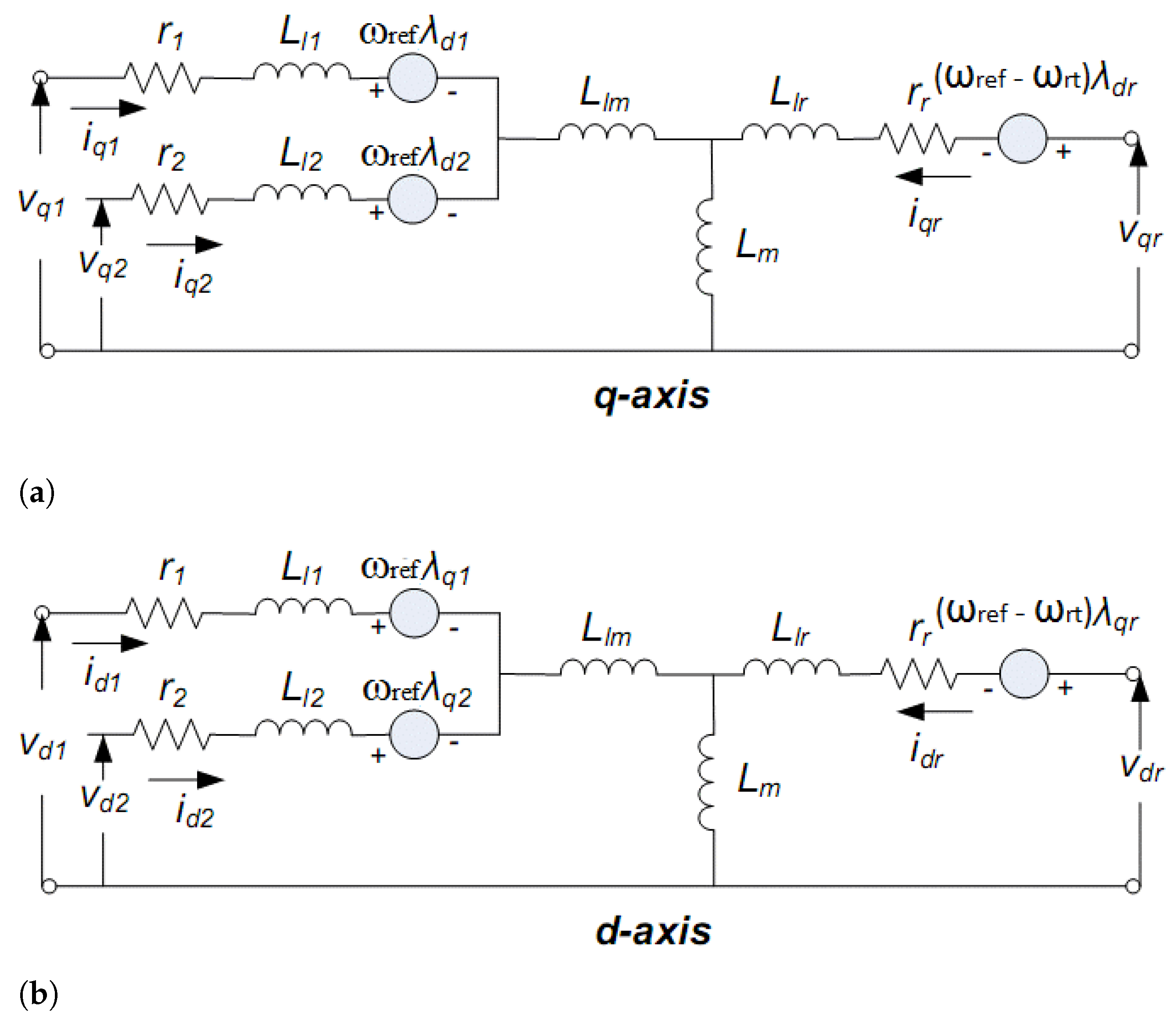
The dynamic equivalent representation was modeled and developed with the assumption of the presence of similar three-phase windings in the stator with their leakage inductance L l 1 and mutual leakage inductance L l m . The equivalent circuit of the six-phase squirrel cage induction motor is shown in Figure 1.
The flux linkage equations are given below [20].
ψ q 1 = L l 1 i q 1 + L l m ( i q 1 + i q 2 ) + L m q ( i q 1 + i q 2 + i q r )
ψ d 1 = L l 1 i d 1 + L l m ( i d 1 + i d 2 ) + L m d ( i d 1 + i d 2 + i d r )
ψ q 2 = L l 2 i q 2 + L l m ( i q 1 + i q 2 ) + L m q ( i q 1 + i q 2 + i q r )
ψ d 2 = L l 2 i d 2 + L l m ( i d 1 + i d 2 ) + L m d ( i d 1 + i d 2 + i d r )
ψ q r = L l r i q r + L m q ( i q 1 + i q 2 + i q r )
ψ d r = L l r i d r + L m d ( i d 1 + i d 2 + i d r )
where
ψ q 1 , ψ q 2 are stator q-axis flux linkage components,
ψ d 1 , ψ d 2 are stator d-axis flux linkage components,
ψ q r , ψ d r are rotor q-axis and d-axis flux-linkage components,
i q 1 , i q 2 are stator q-axis current components,
i d 1 , i d 2 are stator d-axis current components,
i q r , i d r are rotor q-axis and d-axis current components,
L l 1 , L l 2 are stator leakage inductances,
L m q is the air gap inductance of the q-axis,
L m d is the air gap inductance of the d-axis,
L m is the air gap inductance,
L l m is stator mutual leakage inductance, and
L l r is rotor leakage inductance.
The above equation suggests the overall equivalent circuit of the six-phase squirrel cage induction motor shown in Figure 1.
Substituting the flux linkage expressions, Equations (13)–(18), into voltage Equations (7)–(12), to drive the dependence of the voltages on the current in the rotating reference frame, we obtain the following: First, assume the following for simplicity [20].
L m = L m q = L m d
L 1 = L l 1 + L l m + L m
L 2 = L l m + L m
L 3 = L l 2 + L l m + L m
L r = L l r + L m
Substituting Equations (13) and (14) into Equation (7), then the following is obtained.
V q 1 = R s 1 i q 1 + ω k ( L l 1 i d 1 + L l m ( i d 1 + i d 2 ) + L m d ( i d 1 + i d 2 + i d r ) ) + p ( L l 1 i q 1 + L l m ( i q 1 + i q 2 ) + L m q ( i q 1 + i q 2 + i q r ) )
By rearranging the above equation, the following is obtained.
V q 1 = R s 1 i q 1 + ω k i d 1 ( L l 1 + L l m + L m d ) + ω k i d 2 ( L l m + L m d ) + ω k i d r L m d + p i q 1 ( L l 1 + L l m + L m q ) + p i q 2 ( L l m + L m q ) + p i q r L m q
Then, substituting Equations (19)–(21) into Equation (25), the following simplified equation is obtained.
V q 1 = R s 1 i q 1 + ω k L 1 i d 1 + ω k L 2 i d 2 + ω k L m i d r + L 1 p i q 1 + L 2 p i q 2 + L m p i q r
Substituting Equations (13) and (14) into Equation (8), then the following is obtained.
V d 1 = R s 1 i d 1 ω k ( L l 1 i q 1 + L l m ( i q 1 + i q 2 ) + L m d ( i q 1 + i q 2 + i q r ) ) + p ( L l 1 i d 1 + L l m ( i d 1 + i d 2 ) + L m q ( i d 1 + i d 2 + i d r ) )
By rearranging the above equation, then the following is obtained.
V d 1 = R s 1 i d 1 ω k i q 1 ( L l 1 + L l m + L m d ) ω k i q 2 ( L l m + L m d ) ω k i q r L m d + p i d 1 ( L l 1 + L l m + L m q ) + p i d 2 ( L l m + L m q ) + p i d r L m q
Then, substituting Equations (19)–(21) into Equation (28), the following simplified equation is obtained.
V d 1 = R s 1 i d 1 ω k L 1 i q 1 ω k L 2 i q 2 ω k L m i q r + L 1 p i d 1 + L 2 p i d 2 + L m p i d r
Substituting Equations (15) and (16) into Equation (9), then the following is obtained.
V q 2 = R s 2 i q 2 + ω k ( L l 2 i d 2 + L l m ( i d 1 + i d 2 ) + L m d ( i d 1 + i d 2 + i d r ) ) + p ( L l 2 i q 2 + L l m ( i q 1 + i q 2 ) + L m q ( i q 1 + i q 2 + i q r ) )
By rearranging the above equation, the following equation is obtained.
V q 2 = R s 2 i q 2 + ω k ( L l m + L m d ) i d 1 + ω k ( L l 2 + L l m + L m d ) i d 2 + ω k L m d i d r + p i q 2 ( L l 2 + L l m + L m q ) + p i q 1 ( L l m + L m q ) + p i d r L m q
Then, substituting Equations (19), (21), and (22) into Equation (31), the following simplified equation is obtained.
V q 2 = R s 2 i q 2 + ω k L 2 i d 1 + ω k L 3 i d 2 + ω k L m i d r + L 3 p i q 2 + L 2 p i q 1 + L m p i d r
Substituting Equations (15) and (16) into Equation (10), the following equation is obtained.
V d 2 = R s 2 i d 2 ω k ( L l 2 i q 2 + L l m ( i q 1 + i d 2 ) + L m d ( i q 1 + i q 2 + i q r ) ) + p ( L l 2 i d 2 + L l m ( i d 1 + i d 2 ) + L m q ( i d 1 + i d 2 + i d r ) )
By rearranging the above equation, the following equation is obtained.
V d 2 = R s 2 i d 2 ω k ( L l m + L m d ) i q 1 ω k ( L l 2 + L l m + L m d ) i q 2 ω k L m d i q r + p i d 2 ( L l 2 + L l m + L m q ) + p i d 1 ( L l m + L m q ) + p i d r L m q
Then, substituting Equations (19), (21) and (22) into Equation (34), the following simplified equation is obtained.
V d 2 = R s 2 i d 2 ω k L 2 i q 1 ω k L 3 i q 2 ω k L m i q r + L 3 p i d 2 + L 2 p i d 1 + L m p i d r
Substituting Equations (17) and (18) into Equation (11), the following equation is obtained.
V q r = R r i q r + ( ω k ω r ) ( L l r i d r + L m d ( i d 1 + i d 2 + i d r ) ) + p ( L l r i q r + L m q ( i q 1 + i q 2 + i q r ) )
By rearranging the above equation, the following equation is obtained.
V q r = R r i q r + ( ω k ω r ) L m d i d 1 + ( ω k ω r ) L m d i d 2 + ( ω k ω r ) ( L l r + L m d ) i d r + L m q p i q 1 + L m q p i q 2 + ( L l r + L m q ) p i d r
Then, substituting Equations (19) and (23) into Equation (37), the following simplified equation is obtained.
V q r = R r i q r + ( ω k ω r ) L m i d 1 + ( ω k ω r ) L m i d 2 + ( ω k ω r ) L r i d r + L m p i q 1 + L m p i q 2 + L r p i q r
Substituting Equations (17) and (18) into Equation (12), the following equation is obtained.
V d r = R r i d r ( ω k ω r ) ( L l r i q r + L m d ( i q 1 + i q 2 + i q r ) ) + p ( L l r i d r + L m q ( i d 1 + i d 2 + i d r ) )
By rearranging the above equation, the following equation is obtained.
V d r = R r i d r ( ω k ω r ) ( L m q ) i q 1 ( ω k ω r ) L m q i q 2 ( ω k ω r ) ( L l r + L m q ) i q r + L m d p i d 1 + L m d p i d 2 + ( L l r + L m d ) p i d r
Then, substituting Equations (19) and (23) into Equation (40), the following simplified equation is obtained.
V d r = R r i q r ( ω k ω r ) L m i q 1 ( ω k ω r ) L m i q 2 ( ω k ω r ) L r i q r + L m p i d 1 + L m p i d 2 + L r p i d r
Now, rewriting Equations (26), (29), (32), (35), (38), and (41) in the following manner:
V q 1 = R s 1 i q 1 + ω k L 1 i d 1 + 0 i q 2 + ω k L 2 i d 2 + 0 i q r + ω k L m i d r + L 1 p i q 1 + 0 p i d 1 + L 2 p i q 2 + 0 p i d 2 + L m p i q r + 0 p i d r
V d 1 = R s 1 i d 1 ω k L 1 i q 1 ω k L 2 i q 2 + 0 i d 2 ω k L m i q r + 0 i d r + 0 p i q 1 + L 1 p i d 1 + 0 p i q 2 + L 2 p i d 2 + 0 p i q r + L m p i d r
V q 2 = 0 i q 1 + ω k L 2 i d 1 + R s 2 i q 2 + ω k L 3 i d 2 + 0 i q r + ω k L m i d r + L 2 p i q 1 + 0 p i d 2 + L 3 p i q 2 + 0 p i d 2 + L m p i q r + 0 p i d r
V d 2 = R s 2 i d 2 ω k L 2 i q 1 ω k L 3 i q 2 ω k L m i q r + 0 p i q 1 + L 2 p i d 1 + 0 p i q 2 + L 3 p i d 2 + 0 p i q r + L m p i d r
V q r = 0 i q 1 + ( ω k ω r ) L m i d 1 + 0 i q 2 + ( ω k ω r ) L m i d 2 + R r i d r + ( ω k ω r ) L r i d r + L m p i q 1 + 0 i d 1 + L m p i q 2 + 0 i d 2 + L r p i q r + 0 i d r
V d r = ( ω k ω r ) L m i q 1 + 0 i d 1 ( ω k ω r ) L m i q 2 + 0 i d 2 ( ω k ω r ) L r i q r + R r i d r + 0 p i q 1 + L m p i d 1 + 0 p i q 2 + L m p i d 2 + 0 p i q r + L r p i d r
Now, using state variable method, Equations (42)–(47) can be represented in a state variable form as follows [20].
V q 1 V d 1 V q 2 V d 2 V q r V d r = R s 1 ω k L 1 0 ω k L 2 0 ω k L m ω k L 1 R s 1 ω k L 2 0 ω k L m 0 0 ω k L 2 R s 2 ω k L 3 0 ω k L m ω k L 2 0 ω k L 3 R s 2 ω k L m 0 0 ( ω k ω r ) L m 0 ( ω k ω r ) L m R r ( ω k ω r ) L r ( ω k ω r ) L m 0 ( ω k ω r ) L m 0 ( ω k ω r ) L r R r
* i q 1 i d 1 i q 2 i d 2 i q r i d r + L 1 0 L 2 0 L m 0 0 L 1 0 L 2 0 L m L 2 0 L 3 0 L m 0 0 L 2 0 L 3 0 L m L m 0 L m 0 L r 0 0 L m 0 L m 0 L r p i q 1 p i d 1 p i q 2 p i d 2 p i q r p i d r
or in a simple form X = AI + B ρ I, where
A = R s 1 ω k L 1 0 ω k L 2 0 ω k L m ω k L 1 R s 1 ω k L 2 0 ω k L m 0 0 ω k L 2 R s 2 ω k L 3 0 ω k L m ω k L 2 0 ω k L 3 R s 2 ω k L m 0 0 ( ω k ω r ) L m 0 ( ω k ω r ) L m R r ( ω k ω r ) L r ( ω k ω r ) L m 0 ( ω k ω r ) L m 0 ( ω k ω r ) L r R r
B = L 1 0 L 2 0 L m 0 0 L 1 0 L 2 0 L m L 2 0 L 3 0 L m 0 0 L 2 0 L 3 0 L m L m 0 L m 0 L r 0 0 L m 0 L m 0 L r

2.1.1. Mechanical Model

The mechanical model of a six-phase induction machine is the equation of motion of the machine and the driven load, written as [20];
J m p 2 θ m = T e B T L
The combined rotor and load viscous friction (B) is appropriately zero, so that the following equation is obtained from Equation (48).
J m d d t 2 2 θ m = T e T L
Now, decomposing Equation (49) into two first-order differential equations gives the following result. Since
d d t ( θ m ) = ω m
therefore the following result is obtained.
J m d d t ( d d t ( θ m ) ) = ( T e T L )
Substituting Equation (50) into Equation (51), the following equation is obtained.
J m d d t ω m = ( T e T L )
From
ω r = ω m d d t
and
θ r = θ m d d t
where
ω m = angular velocity of the rotor,
θ m = rotor angular position,
θ r = electrical rotor angular position,
ω r = electrical angular velocity,
J m = combined rotor and load inertia coefficient, and
T L = load torque.
According to [21], electromagnetic torque is calculated as:
T e = 6 2 P 2 ( λ d s i q s λ q s i d s )
and the drive movement is calculated as follows [22]:
J m d d t ω m + B ω m = T e T L
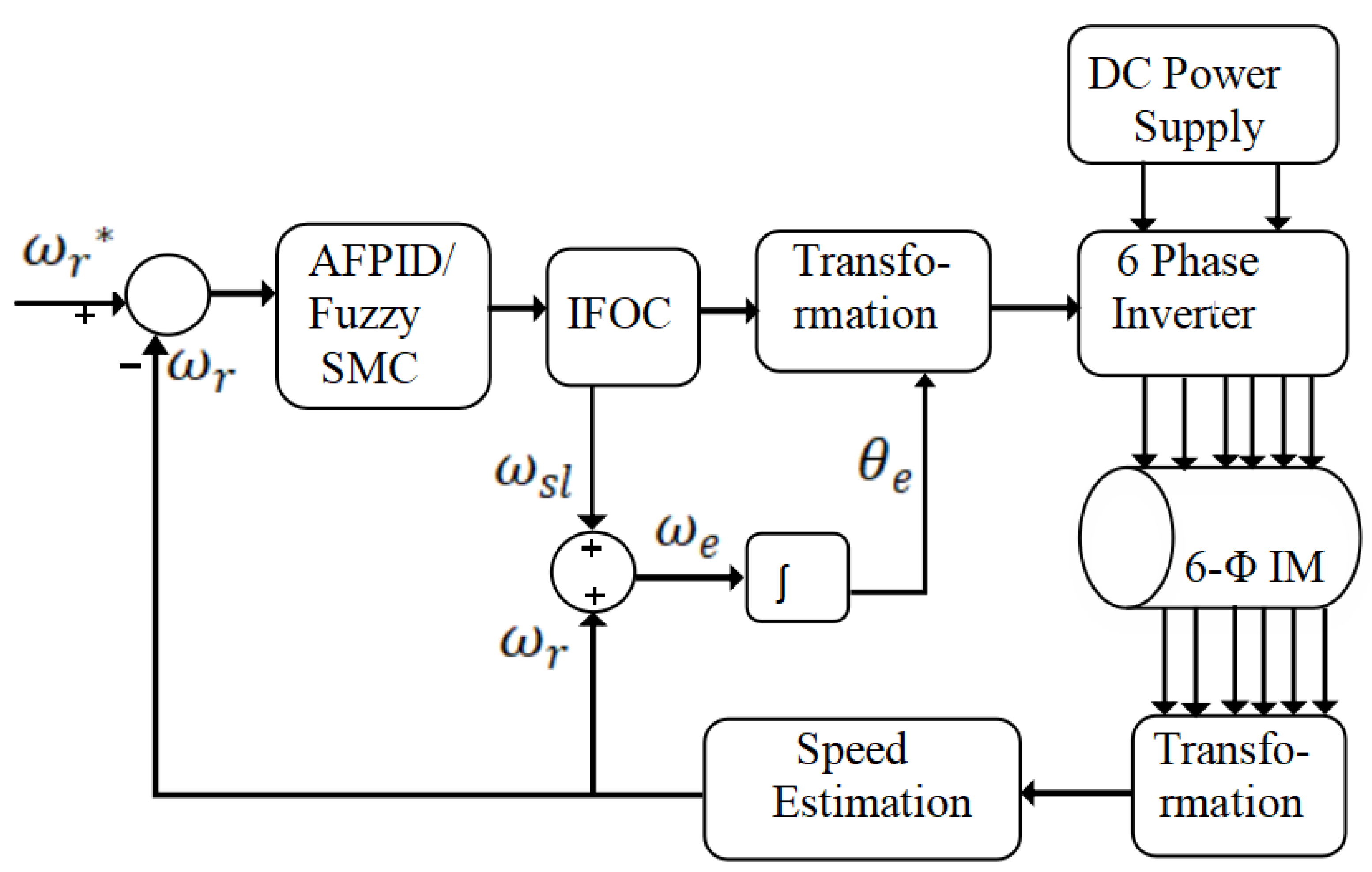
According to indirect field-oriented control (IFOC) techniques, the six-phase induction motor electromechanical torque is obtained as [23];
T e = K t λ d r i q s

2.1.2. PID Controller Design

A continuous PID and a discrete PID are the two types of integral PID speed controllers. The speed controllers employed in this simulation were both the continuous type. In general, series controllers are favored over feedback controllers because higher-order systems require a large number of state variables to detect during feedback, which necessitates a large number of transducers. As a result, series controllers are widely used. The lower-order model is connected to the controller, and the response of the closed loop is observed. The parameters of the controllers are tuned to provide a response that meets the desired specification standards. For the stability process, the parameters of controllers that were tuned are introduced into the higher-order system [24]. For the continuous system, the PID controller transfer function is given as;
G c ( s ) = K p + K i s + K d s
To meet the required performance specification, the determination of the constant values of the proportional gain ( K p ), integral gain ( K i ), and derivative gain ( K d ) are involved in the design. Because the original system transfer function is a higher-order system, we must reduce it to a lower-order system that keeps the important properties of the original system and approximates the response almost the same for the same inputs. In order to find the reduced-order model transfer function from the original higher-order system, the following process is used.
Consider an nth-order linear time-invariant stable system stated by the following transfer function.
G ( s ) = N ( s ) D ( s ) = a 0 + a 1 s + a 2 s 2 + + a i s i b 0 + b 1 s + b 2 s 2 + + b i s i
where a i and b i 0 .
The kth-order reduced model of the corresponding stable system is given in the following form.
M ( s ) = N r ( s ) D r ( s ) = d 0 + d 1 s + d 2 s 2 + + d i s i e 0 + e 1 s + e 2 s 2 + + e i s i
where d i and e i 0 .
Hence, G(s) = M(s).
a 0 + a 1 s + a 2 s 2 + + a i s i b 0 + b 1 s + b 2 s 2 + + b i s i = d 0 + d 1 s + d 2 s 2 + + d i s i e 0 + e 1 s + e 2 s 2 + + e i s i
By criss-cross multiplication and re-arranging Equation (61),
a 0 e 0 + ( a 0 e 1 + a 1 e 0 ) s + ( a 0 e 2 + a 1 e 1 + a 2 e 0 ) s 2 + + a n 1 e k s n 1 + k = b 0 d 0 + ( b 0 d 1 + b 1 d 0 ) s + ( b 0 d 2 + b 1 d 1 + b 2 d 0 ) s 2 + + b n d k 1 s n 1 + k
The following relations are obtained by equating the coefficients of the corresponding terms.
a 0 e 0 = b 0 d 0
a 0 e 1 + a 1 e 0 = b 0 d 1 + b 1 d 0
a 0 e 2 + a 1 e 1 + a 2 e 0 = b 0 d 2 + b 1 d 1 + b 2 d 0
a 0 e k 1 + a 1 e k 2 + a 2 e k 3 + = b 0 d k 1 + b 1 d k 2 + b 2 d k 3 +
a 0 e k + a 1 e k 1 + a 2 e k 2 + = b 1 d k 1 + b 2 d k 2 + b 3 d k 3 +
a 1 e k + a 2 e k 1 + a 3 e k 2 + = b 2 d k 1 + b 3 d k 2 + b 4 d k 3 +
a n 1 e k = b n d k 1
By taking any positive values either for d 0 or e 0 , the unknown parameter values are determined based on the above relation. For simplicity, let us choose either d 0 or e 0 = 1, and substituting in the above relations, the unknown parameter values are obtained. The stability of the reduced-order model system is checked by the Routh–Hurwitz criteria.
The original higher-order derived system is the fourth-order system transfer function, given as follows.
G ( s ) = 2.789 s 3 + 253.4 s 2 + 7026 s + 5.404 e 04 s 4 + 103.5 s 3 + 3672 s 2 + 5.133 e 04 s + 2.458 e 05
then consider the reduced second-order transfer function given by the following representations.
G ( s ) = d 1 s + d 0 e 2 s 2 + e 1 s + e 0
Now, equating G(s) with M(s) together and cross-multiplying, the following equation is obtained.
( 2.789 s 3 + 253.4 s 2 + 7026 s + 54040 ) ( d 0 + d 1 s ) = ( s 4 + 103.5 s 3 + 3672 s 2 + 51330 s + 245800 ) ( e 02 + e 1 s + e 2 s 2 )
2.789 e 0 s 3 + 253.4 e 0 s 2 + 7026 e 0 s + 54040 e 0 + 2.789 e 1 s 4 + 253.4 e 1 s 3 + 7026 e 1 s 2 + 54040 e 1 s + 2.789 e 2 s 5 + 253.4 e 2 s 4 + 7026 e 2 s 3 + 54040 e 2 s 2 = d 0 s 4 + 103.5 d 0 s 3 + 3672 d 0 s 2 + 51330 d 0 s + 245800 d 0 + d 1 s 5 + 103.5 d 1 s 4 + 3672 d 1 s 3 + 51330 d 1 s 2 + 245800 d 1 s
By re-arranging and equating the corresponding terms, then the following relations are obtained.
54040 e 0 = 245800 d 0
7026 e 0 + 54040 e 1 = 51330 d 0 + 245800 d 1
253.4 e 0 + 7026 e 1 + 54040 e 2 = 3672 d 0 + 51330 d 1
2.789 e 0 + 253.4 e 1 + 7026 e 2 = 103.5 d 0 + 3672 d 1
2.789 e 1 + 253.4 e 2 = d 0 + 103.5 d 1
2.789 e 2 = d 1
Now, for simplicity, let us choose d 0 = 1, and solving Equation (74), the following relation is obtained.
54040 e 0 = 245800
Solving for e 0 results in
e 0 = 4.55
A standard second-order transfer function has a unity coefficient; therefore, the e 2 value is 1.
e 2 = 1
From Equation (79), substituting the value of e 2 , the value of d 1 is obtained.
d 1 = 2.789
By substituting the values of e 0 , e 2 , d 0 , and d 1 into Equation (75) and solving, the following value of e 1 is obtained.
e 1 = 13.044
Now, the reduced-order transfer function is written as follows.
G ( s ) = d 1 s + d 0 e 2 s 2 + e 1 s + e 0
Substituting the values of the parameters, the following equation is obtained.
G ( s ) = 2.789 s + 1 s 2 + 13.044 s + 4.55
With the open-loop transfer function G(s), its closed-loop transfer function of a unity feedback system is given in Equation (86).
T F ( s ) = G ( s ) 1 + G ( s )
If the system performance requirements (e.g., output response) do not fulfill the desired specifications, a PID controller is attached to the original open-loop system, and its closed-loop transfer function is given in Equation (87).
T F c ( s ) = G c o n t ( s ) G ( s ) 1 + G c o n t ( s ) G ( s )
where G c o n t ( s ) is the transfer function of the PID controller.
The initial values of the proportional gain, integral gain, and derivative gain are obtained by using a pole zero cancellation applied to the reduced-order system. Using the initial values of the proportional gain, integral gain, and derivative gain, these initial values are tuned to obtain a unit response of the compensated system that satisfies the desired specifications. After tuning of these variables, the new tuned values are obtained, which are given in Table 1.

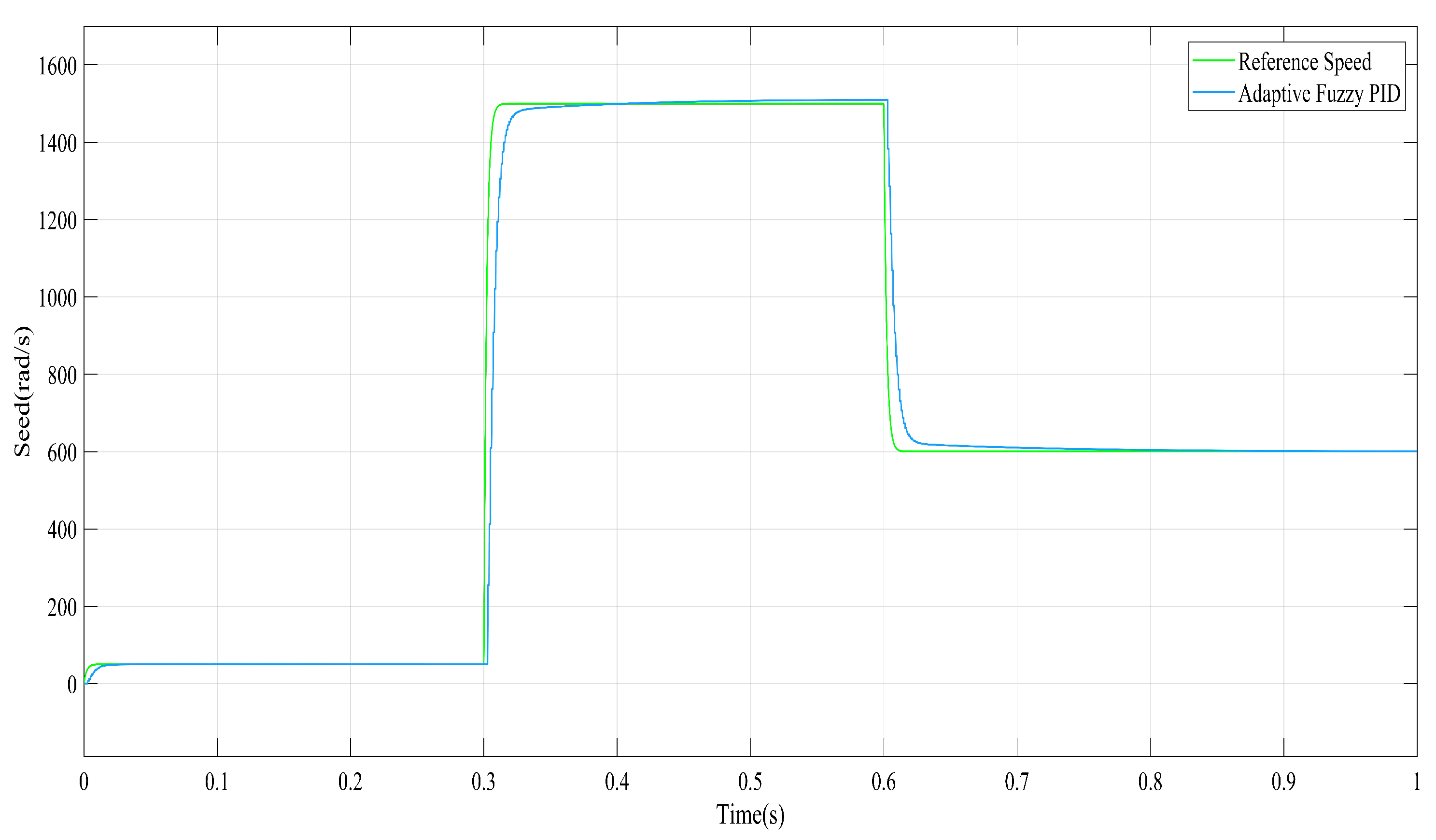
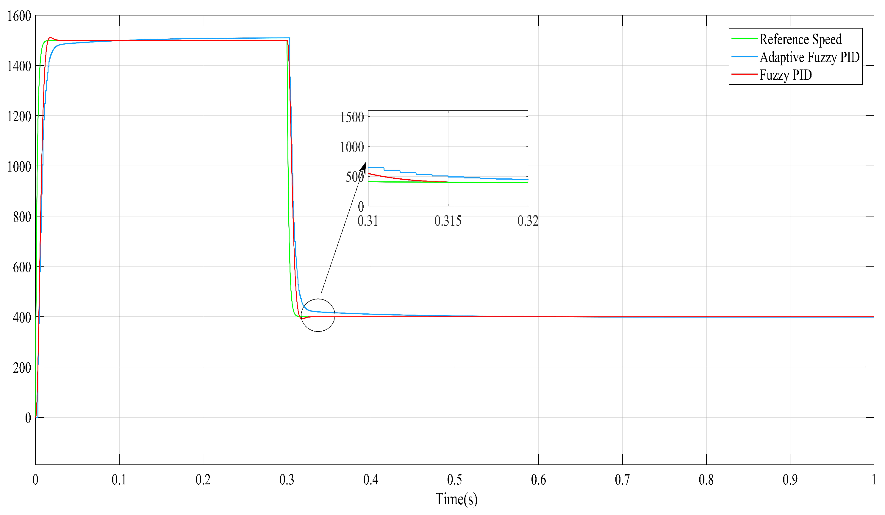
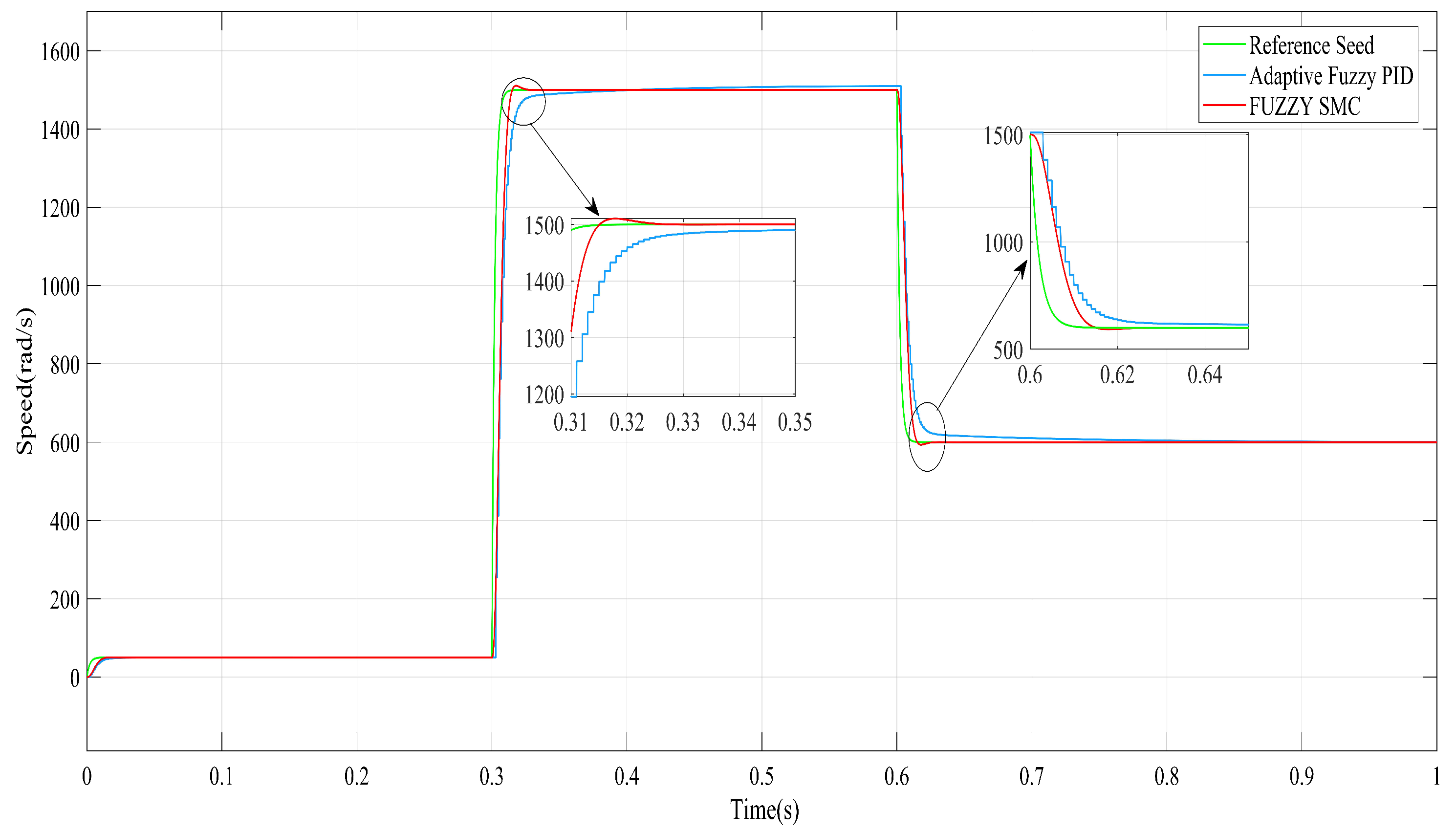
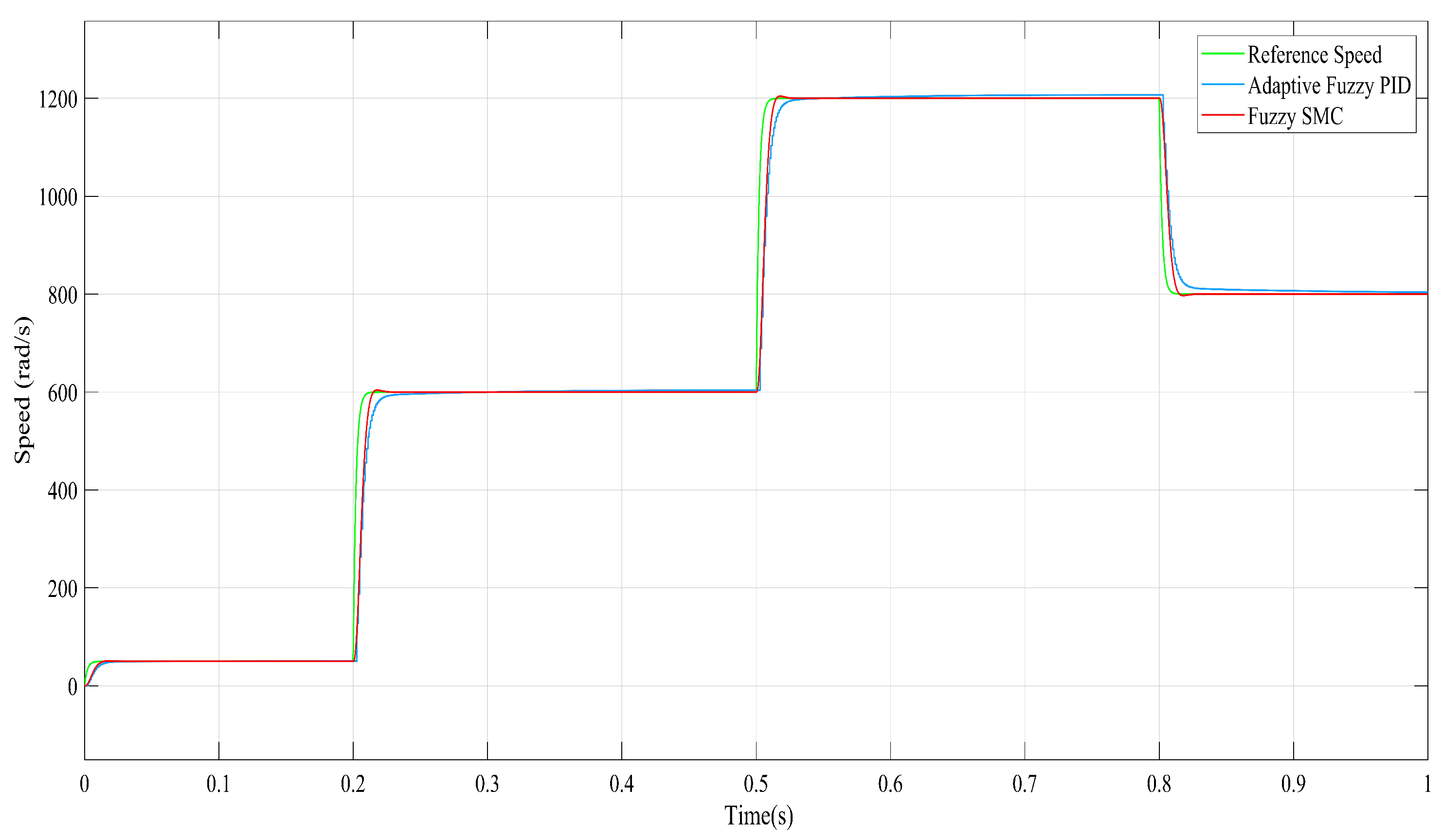
2.1.3. Adaptive Fuzzy PID Controller

The fuzzy PID is a hybrid controller that combines PID and fuzzy logic controllers [25,26]. This combined controller has the ability to adapt to any situation, such as the rising quantity of the input changes. The adaptive fuzzy PID controller’s main goals are to simplify the control techniques and improve the system’s static and dynamic performance, in particular for systems with complex parameters. In this scenario, the adaptive fuzzy controller is programmed to alter the PID parameters K p , K i , and K d to achieve the desired characteristics, such as the overshoot, rising, and settling time and steady-state error [27]. As a result, the PID controller’s proportional integral and derivative actions will be used to construct the fuzzy logic controller’s control signal [28]. There are two inputs and one output in fuzzy logic control. These are, respectively, the error (e), error change ( e c ), and control signal. Linguistic variables that imply the inputs and output have been classified as: NB, NM, NS, Z, PS, PM, and PB [29]. The adaptive fuzzy PID controller is based on two inputs and three outputs. The error speed (e) and change in error speed ( e c ) are the fuzzy control inputs, and the fuzzy outputs are Δ K p , Δ K i , and Δ K d .
Δ K p = K p × Δ K p *
Δ K i = K i × Δ K i *
Δ K d = K d × Δ K d *

The Control Rules of Fuzzy Controller

The three PID arithmetic parameters will affect the system’s stability, response speed, overshoot, and stable precision:
  • If | e | is small, the large values of Δ K p and Δ K i are thought to ensure system stability.
  • If | e | is medium, a small value of Δ K p and an appropriate value of K i are considered to increase the performance response in the situation of reducing the overshoot.
  • If | e | is large, then values of Δ K p and Δ K i equal zero are needed to have a good settling time, a good rise time, and a good overshoot.
There are seven fuzzy sets for K p control, for a total of 49 fuzzy rules in Table 2 and these rules in the table are transferred into numbers as in Table 3.
Table 3 shows a K p seven-valued function.
There are seven fuzzy sets for K i control, for a total of 49 fuzzy rules in Table 4 and these rules in the table are transferred into numbers as in Table 5.
Table 5 shows a K i seven-valued function.
There are seven fuzzy sets for K d control, for a total of 49 fuzzy rules in Table 6 and these rules in the table are transferred into numbers as in Table 7.
Table 7 shows a K d seven-valued function.

Membership Function of Linguistic Variable

The fuzzy rules are extracted from fundamental information and human experience about the process. The inputs are normalized in the range [−3, 3], and the outputs are the K p interval [−0.3, 0.3], K i interval [−0.06, 0.06], and K d interval [−0.3, 0.3]. Negative big (NB), negative medium (NM), negative small (NS), zero (Z), positive small (PS), positive medium (PM), positive big (PB) were the linguistic labels used to characterize the fuzzy sets (PM = 0.3, PM = 0.2, PS = 0.1, Z = 0, NS = −0.1, NM = −0.2, and NB = −0.3). These rules describe the control strategy by defining the input and output relationships. There are seven fuzzy sets for each control input, for a total of 49 fuzzy rules.

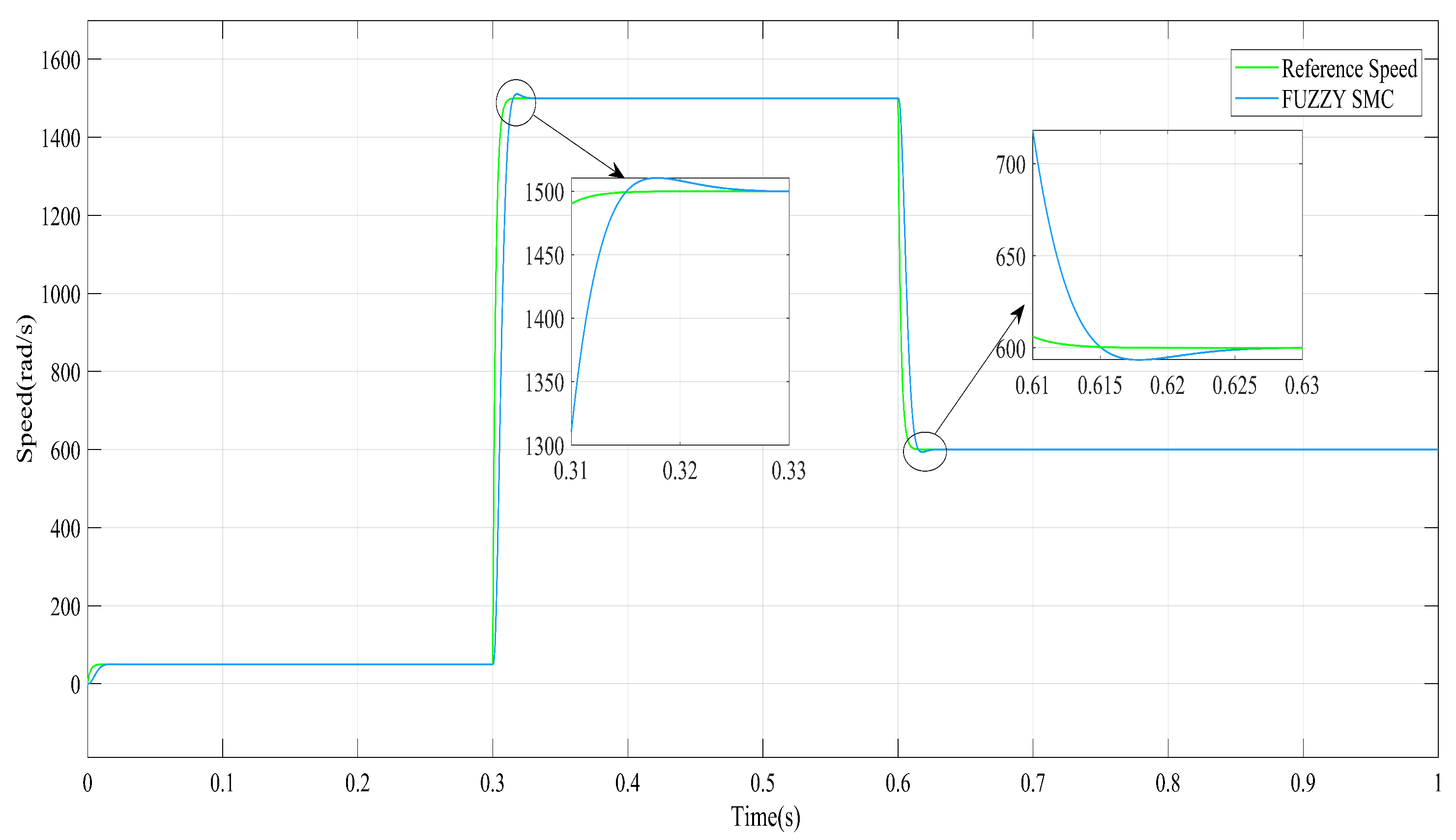
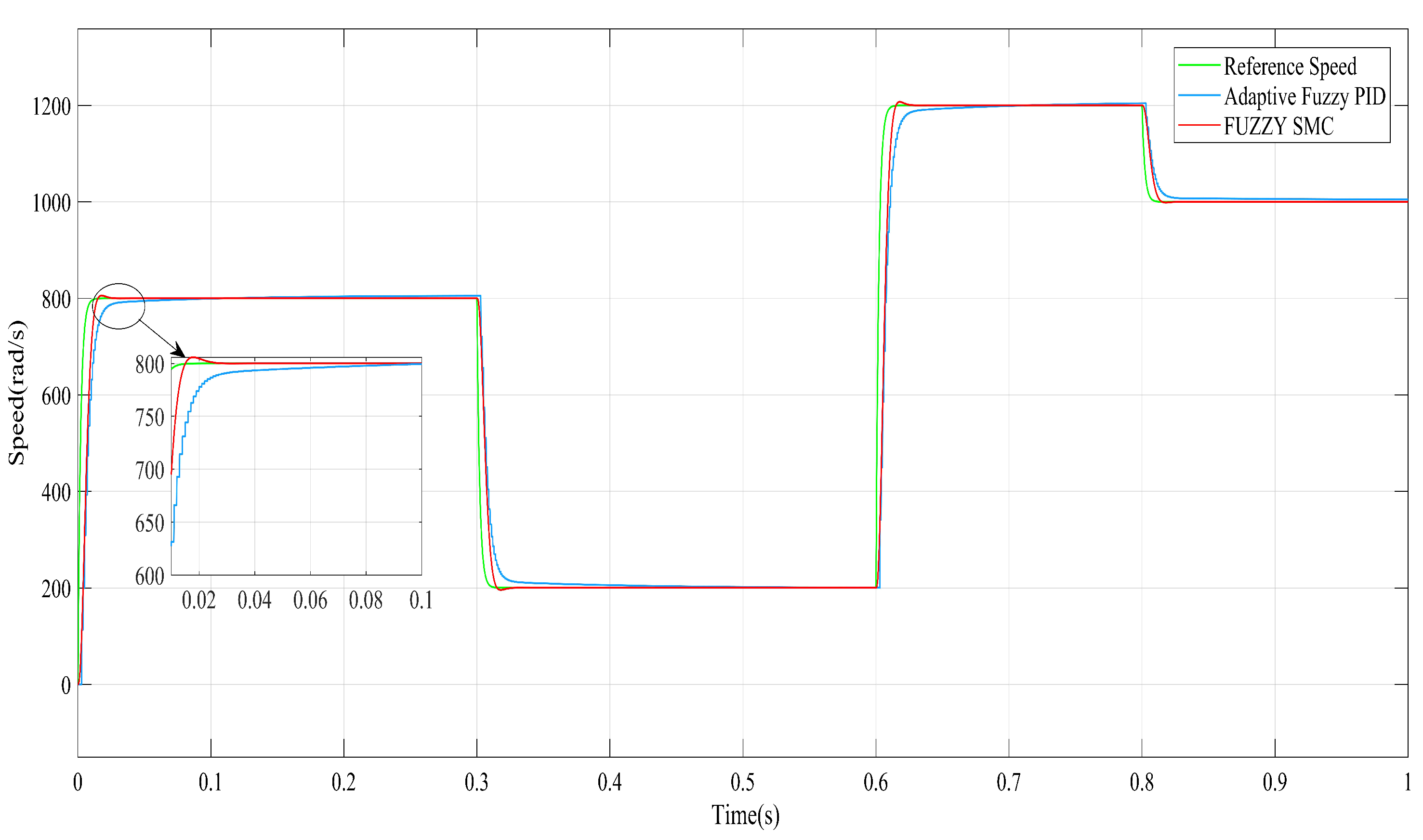
2.1.4. Proposed Fuzzy Sliding Mode Controller

Sliding mode control (SMC) has been used in linear and nonlinear controls. A sliding mode control with a variable control structure is taken as an adaptive observer, which gives the good performance of the drive system with parameter variation and load torque disturbance. The concept of SMC is that the drive response is forced to track or slide the predefined sliding surface. Sliding mode control (SMC) was utilized to create the state observer and as a tracking trajectory for the response of the drive system as the reference model signal. The sliding surface design was focused on to fulfil the reachability condition of the drive system [30,31]. The control problem obtains the motor speed to track a specific time-varying command in the presence of model imprecision, load torque disturbances, and measurement noise. In SMC, the system is intended to minimize the tracking error in the way that e = ω r ω r * , and its rate of change always moves towards a sliding surface. The sliding surface is defined in the state space by the scalar equation [32]. S ( e , e , t ) = 0 where the sliding variable, s, is:
s = e + λ e
where λ is a positive constant that depends on the bandwidth of the system. The tracking problem is similar to staying on the sliding surface indefinitely, with the sliding variable s set to zero. The switching surface of a second-order system is a line. The system state is driven onto the switching line by the control input, and once there, the system is limited to stay on the line. The control input is determined by the error trajectory’s distance from the sliding surface and its rate of convergence. At the point where the tracking error trajectory meets the sliding surface, the sign of the control input must change. As a result, the error trajectory is compelled to follow the sliding surface at all times. The system is forced to slide down the sliding surface to the equilibrium point once it reaches the sliding surface. The condition of the sliding mode is [33]:
1 2 d d t s 2 = s s η s
where η is a positive constant.
Equation (89) is stricter than the general sliding condition: s s 0, and it is equivalent to
s s g n ( s ) η
To design a sliding mode speed controller for an induction motor drive system, the steps are as follows. Substitute (88) involving the speed error e in (90):
ω r + λ e ω r s g n ( s ) η
The speed dynamics is given by
J ω r + B ω r + T L = T e = K T ϕ α r i β s
Equivalently, (92) can be expressed as
ω r = g 1 T L J
where g 1 = B ω r + K T ϕ α r i β s J is a function.
Differentiating (93) with respect to time and simplifying:
ω r = G b v β s
where
G = B g 1 + K T ϕ α r g 2 J
g 2 = ( a 1 + τ r 1 ) ρ ω r ( 1 + a 3 L m ) i α s
b = K T ϕ α r σ L s J
G is a function that may be calculated from the current and speed measurements, and d is the disturbance caused by the load torque, as well as an error in G estimates caused by measurement imperfections. The control effort is the third term, because the q-axis stator voltage command is in charge of adjusting the torque. There is no measurement or estimation in the most basic sliding mode controller. It does not consider G in any way.
It is defined as
v β s * = k ( s a t ) ϕ
where ( s a t ) ϕ is given as follows
( s a t ) ϕ = s ϕ , if | s | ϕ . s g n ( s ) , if | s | ϕ .
The parameters of sliding mode controllers are K = 1800, λ = 2, and δ = 0.15 .

2.2. Speed Observer Design

Sensorless speed control needs to design an observer to estimate the speed via a feedback loop with measured plant parameters. To estimate the speed, the model reference adaptive controller (MRAC) was used, in which the observer is used as an adaptive model. This observer was modeled based on machine d-q model of measurable variables such as stator currents i r d , i r q and rotor fluxes ψ r d , ψ r q .
The state-space representation of the dynamic system was used to design observer with gain to adjust the output error to achieve the desired fast estimated signal. The linear time-invariant system can be expressed as:
X = A x + B U
Y = C x
where x = [ i r d i r q ψ r d ψ r q ] T are the state variables in terms of the stator current and rotor flux and A, B, C, U, Y are the matrix values derived from the induction motor. Using the voltage equations of the squirrel cage induction motor in the stator frame to set up a back e m f observer, the induced back emf components, [ ψ d ψ q ] , can be considered as the disturbance with the following associated model:
d ψ d d t = 0
d ψ q d t = 0
From the equations, the extended model in the general reference model state-space representation is given as:
x ^ e = A e x ^ e + B e u
y ^ e = C e x ^ e
where x ^ e = [ i d s i q s ϕ d s ϕ q s ] , vector state variables u = [ v d v q ] T , and input vectors A e , B e , C e are the matrices of the system parameters. The error dynamics of the observer is expressed as:
x ^ e = A e x ^ e + B e u + K ( y y ^ e ) = x ^ e = A e x ^ e + B e u + K ( y C e x ^ e )
where y = [ i d , i q ] T is the output vector and K is the observer gain matrix.

2.3. Stability Analysis of the Proposed System

The adaptive model was designed based on the observer state-space model, which updates the rotor fluxes and stator currents, which are used for rotor speed adaptation. However, the estimation should be responsible for the stability of the observation, which can be best performed by determining the error dynamics and system stability, which were checked by the Lyapunov stability criterion. The Lyapunov function (V) used here to check the stability of the estimated rotor speed is
V = e T e + ( ω r ω ^ r ) c
The time derivative of the Lyapunov function ( V ) is given by:
d V d t = [ e T C ( A K C ) C T + C ( A K C ) C T ] e + 2 L m ( ω r ω ^ r ) γ L s L r ( e r q e r d ) + 2 ( ω r ω ^ r ) c d ω ^ r d t
where the q-axis flux error e r q = ϕ r q ϕ ^ r q , d-axis flux error e r d = ϕ r d ϕ ^ r d , and γ = 1 ( L m ) 2 L s L r is a coupling factor. The total flux error is therefore:
e ϕ r = e r q e r d
where K is the observer gain selected to obtain a fast response to compromise the estimation error and obtained from
d e t ( A K I ) = A
By the selection of observer gain (K) using the equivalence principle, which states that the observer pole location is selected by direct comparison, the observer poles are proportional to the motor poles. The distinctive nature or features of this observer gain are by an equation having a term that adjusts the current state estimates by an amount proportional to the prediction error, subtracting the actual measurement from the estimation of the current output. This correction ensures the stability and convergence of the observer even when the system being observed is unstable. The derivative of the Lyapunov function is always negative definite due to the sufficient conditions for asymptotic stability being that V has to decrease when the error is not zero, which means the first term of the above function is always negative definite, since the system is stable [34]. The estimation of the rotor speed can be calculated as:
d ω ^ r d t = L m γ L s L r ( K p e ϕ t o t a l + K i e ϕ t d t )

3. Simulation Results and Discussion

The proposed adaptive fuzzy PID and fuzzy SMC-based sensorless speed control of the six-phase induction motor drive were thoroughly tested in a simulation under a variety of operating situations to illustrate the proposed controller’s efficiency and advantages. The suggested approach was simulated in the MATLAB/Simulink environment to verify its effectiveness. The rated induction motor parameters are given as Table 8.
A six-phase induction motor with a 15 Nm rated torque and 1500 rpm as the rated speed at 50 Hz was used to construct the proposed sensorless six-phase induction motor drive. The motor parameter information is provided in Table 8. A block diagram of the fuzzy-slide-mode-controller-based six-phase induction motor drive is shown in Figure 2. The system consisted of a DC power supply, a six-phase squirrel cage induction motor, an inverter, an indirect field-oriented control, and a (adaptive fuzzy PID and fuzzy SMC) speed controller. The modeling of the six-phase induction motor, inverter, and indirect rotor field-oriented control of the six-phase induction motor made up the control system of the six-phase induction motor drive. For the six-phase induction motor, the indirect field-oriented control theory was used. It is easy to apply the vector control scheme to such an arrangement, and it can quickly decouple the torque and flux. In order to produce the torque component current command in Figure 2, the estimated motor speed was compared to the command speed. The error signal was then processed by the adaptive fuzzy PID and fuzzy SMC controller. The indirect rotor field-oriented control approach that was implemented determines how to compute the flux component current command. The rotor position ( θ e ) was then used to convert the torque component current command and flux component current command into six-phase current commands in the stationary reference frame.
The original higher-order system was attached to the designed PID controller Gcont(s) for improved performance. The closed loop response met the required specification after the PID controller was attached to the original system.
The simulation tests were used to examine the performance of the controller in question while varying the parameters. Different reference torques were taken into account in the simulation results due to the variable loading conditions. The steps of increasing load torque began at t = 0 and progressed to 0, 5, 10, and 20 and 0, 0.3, 0.5, 0.8 and 0.1 s, respectively, with matching variations in the stator and rotor current, torque, and speed. It was assumed that the speed was increased and decreased, starting at 50 rad/s and ending at 1500 rad/s, for this purpose. The following graphs show the simulation results produced using the simulation model in Figure 2 for various speed and load settings.
Figure 3 and Figure 4 show the stator current and rotor current response for the applied electromagnetic torque of Figure 5, respectively. Figure 5 shows that the transient of the load torque was maximum at the speed changes and lasted for 0.05 s. At the first step, the load torque was constant, which was 5 Nm for 0.3 s, then increased to 10Nm and was constant for the next 0.3 s, then fell to 3Nm for the last seconds, and there was a step change of the reference speed from 1500 rad/s for 0.3 s and 600 rad/s for the next 0.2 s. In this case, varying the load torque varied the stator and rotor current and electromagnetic torque, while there was no impact on the measured speed. The electromagnetic torque increased as the load torque increased and decreased as the load torque decreased. The motor generated strong torque in the transient state to capture the appropriate reference speeds, as shown in Figure 5. The motor current was higher in the transient state for the same reference speed values, as shown in Figure 3, and it was at the value that could create the motor’s idle running torque in the steady-state. The stator flux was constant and had the same amplitude in both constant speed zones, except in the transient state, because the V by f ratio was equal and constant at both reference speed values.
Figure 6 shows the measured and reference speed when the adaptive fuzzy PID controller was used. The reference speed was 50 rad/s for 0.3 s and 1500 rad/s for the next 0.3 s. Then, after 0.6 s, the reference speed fell to 600 rad/s and the measured speed varied with the speed reference condition, while the measured speed varied with the speed reference condition, which decreased.
Figure 7 shows the measured and reference speed when adaptive fuzzy SMC controller was used. The reference speed was 50 rad/s for 0.3 s and 1500 rad/s for the next 0.3 s. Then, after 0.6 s, the reference speed fell to 600 rad/s and the measured speed varied with the speed reference condition, while the measured speed varied with the speed reference condition, which decreased and had better performance by the adaptive fuzzy PID controller by following the reference speed.
Figure 8 depicts the results of a series of testing of the step changes in the speed reference. Time from 0 to 0.3 s, speed = 50 rad/s, time from 0.3 s to 0.6 s, speed = 1500 rad/s, and and time from 0.6 s to 1 s, speed = 600 rad/s were used to vary the reference speeds of the motors. The controllers’ performance was measured in terms of speed response in this simulation. It can be seen that with fuzzy SMC, the magnitude of the transient speed oscillations reduced. The results revealed that the fuzzy SMC controller outperformed the adaptive fuzzy PID controller. Finally, the simulation results employing the adaptive fuzzy PID and fuzzy SMC controllers for load torques and speed fluctuations were examined. These results confirmed that the fuzzy SMC controller demonstrated better performance under changing operating environments and presented satisfactory performance.

3.1. Reduction in Speed

Figure 9 shows that the transient of load torque was maximum at the start and at the point of speed changes and lasted for 0.05 s. At the first step, the load torque was constant, which was 1 Nm for 0.3 s, then increased to 5 Nm and was constant for the next 0.2 s, then fell to 3 Nm for the last seconds, and there was a step change by the reference speed from 1500 rad/s for 0.3 s and 400 rad/s for the next 0.7 s. In this case, varying the load torque varied the stator and rotor current and electromagnetic torque, while there was no impact on the measured speed. The electromagnetic torque increased as the load torque increased and decreased as the load torque decreased.
Figure 10 and Figure 11 show the stator current and rotor current of for the applied electromagnetic torque of Figure 9.
Figure 12 shows the measured speed response of the system for adaptive fuzzy PID and fuzzy SMC. It was observed that fuzzy SMC had good transient and steady-state response compared to the adaptive fuzzy PID controller when the speed was high at the start and decreased after some time. The motor was loaded with 5 Nm in the range of 0.3 to 0.8 s. The figure shows that as the load increased, the motor speed decreased. The amount of slip must be corrected by the V/f algorithm in order for the falling motor speed to capture the reference speed again. The observed rotor speed was fed back into the algorithm, which allowed for this correction procedure. The motor produced a torque that was sufficient to meet the load put on its shaft during the loading period, as shown in Figure 9.

3.2. Disturbance of Sudden Load Torque

The devices were in a constant state of operation. Then, the load torque increased from 2 Nm to 5 Nm in 0.3 s. As illustrated in Figure 9, the produced torque increased, but had no effect on the speed characteristic. Then, the load torque reduced from 5 to 3 Nm, as shown in Figure 5. As seen in this figure, the produced torque reduced, but had no effect on the speed characteristic. The developed torque dropped, and the rotor speed was unaffected. For a drive with a load torque of 5 Nm, the drive system’s beginning performance was evaluated. Figure 12 shows the motor speed during the starting transient condition, illustrating that the motor reached the set speed in around 0.015 s for fuzzy SMC and 0.2 s for adaptive fuzzy PID without oscillation. As the motor speed approached the reference speed, the motor phase currents decreased.
As the load increased, the stator current and motor torque increased. For a load variation from zero load to a varied load torque condition, adaptive fuzzy PID and fuzzy SMC had transient oscillations of the torques. When fuzzy SMC was applied, the electromagnet torque, rotor speed, and stator phase currents revealed that the system had strong transient and steady-state responsiveness under various load conditions. At the transient response, which oscillated for 0.15 s, the initial torque was considerable. The motor torque and stator current increased as the load increased, but the rotor speed remained unchanged. It can be seen that the speed closely followed the reference value and was unaffected by the load variations. When fuzzy SMC was employed, the torque had superior performance.
Figure 13 shows the measured and reference speed when the adaptive fuzzy PID and fuzzy sliding mode controller were used. The reference speed was 800 rad/s for 0.3 s and fell to 200 rad/s at 0.3 s. Then, after 0.3 s, the reference speed was constant up to 0.6 s. Starting from 0.6 s, the reference speed increased to 1200 rad/s for the next 0.2 s. Then, after 0.8 s, the reference speed fell to 1000 rad/s, and the measured speed varied with the speed reference condition, which decreased and had better performance than the adaptive fuzzy PID controller by following the reference speed.
By the comparison of the expected outputs in terms of the rising time, overshoot, settling time, and deviation from the reference speed, fuzzy SMC from Figure 13 had better performance when compared to adaptive fuzzy PID.
Figure 14 shows the stator current response to varying speed. The reference speed was 50 rad/s for 0.3 s and 1500 rad/s for the next 0.3 s. Then, after 0.6 s, the reference speed fell to 600 rad/s and the measured speed varied with the speed reference condition, which decreased. At the start, since the load was so small, the stator current was also small, and when the speed increased, the stator current oscillated and increased. At the time of speed reduction, the stator current also reduced following the speed.
Figure 15 shows the rotor current response to varying speed. The reference speed was 50 rad/s for 0.3 s and 1500 rad/s for the next 0.3 s. Then, after 0.6 s, the reference speed fell to 600 rad/s and the measured speed varied with the speed reference condition, which decreased. At the start, since the load was so small, the rotor current was high due to the low resistance and came to stationarity, and when the speed increased, the rotor current oscillated slightly toward stationarity. At the time of speed reduction, the rotor current also reduced and slightly oscillated following the speed.
Figure 16 shows the measured and reference speed when the adaptive fuzzy PID and fuzzy sliding mode controller were used, The reference speed were 50 rad/s for 0.3 s and 1500 rad/s for the next 0.3 s, respectively. Then, after 0.6 s, the reference speed fell to 600 rad/s, and the measured speed varied with speed reference condition, which decreased.

3.3. Increase in Speed

Figure 17 shows the measured and reference speed when the adaptive fuzzy PID controller and fuzzy sliding mode controller were used with increasing speed. The reference speed was 50 rad/s for 0.2 s and increased to 600 rad/s at 0.2 s. Then, after 0.2 s, the reference speed was constant up to 0.5 s. Starting from 0.5 s, the reference speed increased to 1200 rad/s for the next 0.3 s. Then, after 0.8 s, the reference speed fell to 800 rad/s and the measured speed varied with the speed reference condition, which decreased by following the reference speed.
By comparison of the expected outputs in terms of the rising time, overshoot, settling time, and deviation from the reference speed, the fuzzy SMC from Figure 17 had better performance when compared to adaptive fuzzy PID.

3.4. Speed Step Change from 50 to 1500 rad/s

The motor was exposed to a speed step change in the speed command from 50 rad/s to 1500 rad/s at t = 0.3 s to assess its performances. This was performed to analyze the dynamic response of the control system due to an increased speed step change. Figure 16 displays the motor’s measured speed together with an updated speed reference. As can be observed, the motor speed signals accelerated smoothly using fuzzy SMC, having almost nearly zero steady-state error. These findings demonstrated that, when the speed changed, fuzzy SMC had a better measured speed signal than its matching measured adaptive fuzzy PID. Figure 14 and Figure 15, respectively, depict the motor’s stator current and rotor current in response to this change in speed. It should be observed that, when the speed step increased, the frequency of the motor phase currents increased, while the value of the current remained constant since the load was constant. These outcomes demonstrated good behavior with quick step change responses and guarantee the efficacy of the suggested strategy.

3.5. Load Change from 5 to 10 Nm

Another crucial element of the six-phase IM control system is its resilience to disturbances. A step change in the motor load is considered a typical disturbance. A high-performance control system has a fast dynamic response in adjusting its control variables so that the system outputs affected by the load impact will recover to the original status as soon as possible. The motor was subjected to a load impact from 5 Nm to 10 Nm at t = 0.3 s. The motor stator and rotor current signals and developed torque corresponding to the load changes are shown in Figure 3, Figure 4 and Figure 5, respectively. Figure 6 and Figure 7 show the measured motor speed with the speed reference of adaptive fuzzy PID and fuzzy SMC corresponding to the load impact. It can be seen that the motor speed signals decelerated and recovered to their original value with acceptable time with nearly zero steady-state error. These results show a good correlation between the reference speed signal and its corresponding measured speed. It is noted that the values of the motor phase currents increases with the load impact and the frequency of the current was constant because the speed was constant. These results showed the good load disturbance rejection of the proposed system.
From Table 9 and Figure 16, it can be seen that the fuzzy SMC had a better response when compared to the adaptive fuzzy PID controller. The target of this thesis was to reduce the settling time and steady-state error, minimize the overshoot, and improve the efficiency and power factor while keeping the weight and power loss at a minimum. The settling time was fast, and a small overshoot was present in the case of fuzzy SMC; hence, fuzzy SMC had better speed control of the six-phase induction motor.

4. Conclusions

A six-phase induction motor drive was modeled, and the proposed sensorless speed control was designed. The controller performances were presented to demonstrate the effectiveness of the result. There are numerous ways to control motor speed; however, in this study, the suggested approach was developed using the AFPID controller and AFSMC. The aim of the study was to design a controller that would allow the speed of the six-phase induction motor to track specified reference values while the load torque was varied, and the proposed system was tested by considering different operating conditions, such as at no-load and a variable load torque, and the performance of induction motor control has been analyzed under different load conditions. The results showed the good dynamic performance and robustness of the AFSMC with a good rising and a better settling time. The AFSMC part of the torque component current showed a low chattering effect on the sliding surface for torque production. This ensured stability and reduced the effect of parameter variation and ripple torque. The proposed AFSMC showed good performance when compared with the AFPID controller for the speed control of the six-phase induction motor. The obtained findings showed that, in comparison to earlier research, the suggested algorithm was a powerful approach to tracking the variation of the load and speed of the studied motor. It was shown that the algorithm was adaptable to changes in the speed and load torque, and it can ensure a quick reaction with the lowest error. The proposed control technique based on the AFSMC presented a very competitive and promising solution for the control of the six-phase induction motor from the findings. Utilizing the MATLAB/SIMULINK software, modeling studies for the six-phase induction motor were created using space vector pulse width modulation (SVPWM). From the conclusion the following advantages were deduced for the proposed system.
  • A six-phase induction motor that was loaded can be powered successfully by a voltage source called a six-phase SVPWM inverter.
  • It is possible to determine the mechanical speed without a sensor by using the stator currents directly and the quadrature axis components, as well as the motor characteristics.
  • When compared to AFPID, the AFSMC’s performance was improved through a wide range of operation and load circumstances.
  • From the result, the response of the AFSMC was quicker than the AFPID controller with minimum overshoot.

Author Contributions

Methodology, T.A.; conceptualization and software validation L.W.; formal analysis and review, supervision, M.M.; writing, editing, and visualization, A.J. All authors have read and agreed to the published version of the manuscript.

Funding

This research received no external funding.

Institutional Review Board Statement

Not applicable.

Informed Consent Statement

Not applicable.

Data Availability Statement

The data that support the findings of this study are available from the authors upon reasonable request.

Acknowledgments

Polonium International Doctoral Fellowships Program at Gdańsk University of Technology.

Conflicts of Interest

The authors declare no conflict of interest.

Abbreviations

The following abbreviations are used in this manuscript:
ACAlternating current
DCDirect current
SPIMSix-Phase induction motor
V/Fvoltage-to-frequency
AFPIDAdaptive fuzzy proportional integral derivative
PIDProportional integral derivative
FSMCFuzzy sliding mode controller
SMCSliding mode controller
MRACModel reference adaptive controller
Fuzzy SMCFuzzy sliding mode controller
6- Φ IMSi-phase induction motor

References

  1. Shiravani, F.; Alkorta, P.; Cortajarena, J.A.; Barambones, O. An Enhanced Sliding Mode Speed Control for Induction Motor Drives. Actuators 2022, 11, 18. [Google Scholar] [CrossRef]
  2. Du, C.; Yang, C.; Li, F.; Gui, W. A Novel Asynchronous Control for Artificial Delayed Markovian Jump Systems via Output Feedback Sliding Mode Approach. IEEE Trans. Syst. Man Cybern. Syst. 2019, 49, 364–374. [Google Scholar] [CrossRef]
  3. Duran, M.J.; Salas, F.; Arahal, M.R. Bifuration Analysis of Five–Phase Induction Motor Drives with Third Harmonic Injection. Ind. Electron. IEEE Trans. 2008, 55, 2006–2014. [Google Scholar] [CrossRef]
  4. Mira, R.S.; Jacobina, C.B.; Lima, A.M.N. Modeling and analysis of six–phase induction machine under fault condition. In Proceedings of the Power Electronics Conference (COBEP’09), Bonito-Mato Grosso do Sul, Brazil, 27 September–1 October 2009; pp. 824–830. [Google Scholar]
  5. Levi, E. Editorial—Special Issue on Multi-Phase Motor Drives. EPE J. 2009, 14, 4. [Google Scholar]
  6. Bugenis, S.J.; Vanagas, J.; Gečys, S. Optimal phase number of induction motor with the integrated frequency converter. Electron. Electr. Eng. Kaunas Technol. 2008, 8, 67–70. [Google Scholar]
  7. Fitzgerald, A.E. Electrical Machine, 6th ed.; McGraw-Hill: Cambridge, UK, 2012. [Google Scholar]
  8. Guo, Z.; Zhang, Q. The Study on Mathematical Model and Simulation of Asynchronous Motor Considering Iron Loss. J. Phys. Conf. Ser. 2018, 1060, 012085. [Google Scholar] [CrossRef]
  9. Qiao, Z.; Shi, T.; Wang, Y.; Yan, Y.; Xia, C.; He, X. New sliding mode observer for position sensorless control of the permanent-magnet synchronous motor. IEEE Trans. Ind. Electron. 2012, 60, 710–719. [Google Scholar] [CrossRef]
  10. Wang, L.; Zhang, H. Sliding Mode Control with Adaptive Fuzzy Compensation for Uncertain Nonlinear System. Hindawi Math. Probl. Eng. 2018, 2018, 2342391. [Google Scholar] [CrossRef]
  11. Bououden, S.; Chadli, M.; Karimi, H.R. Fuzzy Sliding Mode Controller Design Using Takagi-Sugeno Modelled Nonlinear Systems. Hindawi Publ. Corp. Probl. Eng. 2013, 2013, 734094. [Google Scholar] [CrossRef]
  12. Gadoue, S.M.; Giaouris, D.; Finch, J.W. MRAS sensorless vector control of an induction motor using new sliding mode and fuzzy-logic adaptation mechanisms. IEEE Trans. Energy Convers. 2010, 25, 394–402. [Google Scholar] [CrossRef]
  13. Barrero, F.; Gonzales, A.; Torralba, A.; Galvan, E.; Franquelo, L.G. Speed control of induction motors using a novel fuzzy sliding mode structure. IEEE Trans. Fuzzy Syst. 2003, 10, 375–383. [Google Scholar] [CrossRef]
  14. Kowalska, T.O.; Dybkowski, M.; Szabat, K. Adaptive sliding mode neurofuzzy control of the two-mass induction motor drive without mechanical sensors. IEEE Trans. Ind. Electron. 2010, 57, 553–564. [Google Scholar] [CrossRef]
  15. Huang, C.I.; Hsu, K.C.; Chiang, H.H.; Kou, K.K.; Lee, T.T. Adaptive fuzzy sliding mode control of linear induction motors. In Proceedings of the 2012 International Conference on Advanced Mechatronics Systems, Tokyo, Japan, 18–21 September 2012; pp. 626–631. [Google Scholar]
  16. Cerman, O.; Husek, P. Adaptive fuzzy sliding mode control for electrohydraulic servo mechanism. Expert Syst. Appl. 2012, 39, 10269–10277. [Google Scholar] [CrossRef]
  17. Shahnazi, R.; Shanechi, H.M.; Pariz, N. Position control of induction and DC servomotor: A novel adaptive fuzzy PI sliding mode control. IEEE Trans. Energy Convers. 2008, 23, 138–147. [Google Scholar] [CrossRef]
  18. Kumbhar, P.; Udas, G.; Gandhi, N.; Ghadigaonkar, P.; Randhave, S. Open Loop V/F Control of Six Phase Induction Motor. Int. Res. J. Eng. Technol. IRJET 2021, 8, 750–755. [Google Scholar]
  19. Pal, B.K.; Prajapati, P.; Bajaj, M.; Singh, S. Control of Grid Side Converter for Grid Connected Six Phase Induction Generator. In Proceedings of the IEEE ICCCCM 2013, Allahabad, India, 3–4 August 2013; pp. 1–7. [Google Scholar]
  20. James, A.E.; Anih, L.; Okoro, O. Transient Analysis and Modeling of Sixphase Asynchronous Machine. Am. J. Electr. Power Energy Syst. 2015, 4, 77–83. [Google Scholar] [CrossRef]
  21. Abdelwanis, M.I.; El-Sehiemy, R.A. A Fuzzy-Based Controller of a Modified Six-Phase Induction Motor Driving a Pumping System; Springer: Berlin/Heidelberg, Germany, 2018; Volume 8, pp. 580–587. [Google Scholar] [CrossRef]
  22. Akpama, E.J. Modeling Of Six-Phase Induction Machine Including Saturation Effect. J. Multidiscip. Eng. Sci. Technol. JMEST 2019, 6. [Google Scholar]
  23. Abdel-Khalik, A.S. Postfault Control of Scalar (V/f) Controlled Asymmetrical Six-Phase Induction Machines. IEEE Access 2019, 6, 59211–59220. [Google Scholar] [CrossRef]
  24. Djalal, M.R.; Faisal, F. Design of Optimal PID Controller for Three Phase Induction Motor Based on Ant Colony Optimization. Sinergi 2020, 24, 125–132. [Google Scholar] [CrossRef]
  25. Singh, S.; Sharma, P. Speed Control Analysis and Performance Comparison of Induction Motor Using Improved Hybrid PID Fuzzy Controller. Int. J. Sci. Res. Eng. Trends 2021, 7, 989–993. [Google Scholar]
  26. Singh, S.; Singh, N. Performance and Comparison Analysis of Speed Control of Induction Motor using Improved Hybrid PID Fuzzy Controller. Int. J. Sci. Res. Dev. 2020, 7. [Google Scholar] [CrossRef]
  27. Tola, T.A.; Yuan, Z. Performance and Comparative Analysis of Sliding Mode Control and PID Control for Three Phase Induction Motors. Int. J. Eng. Res. Technol. IJERT 2021, 10, 420–425. [Google Scholar] [CrossRef]
  28. Bidwe Umesh, B.; Shinde Sanjay, M. Speed Control of Three Phase Induction Motor Using Fuzzy-PID Controller. Int. J. Eng. Res. Technol. IJERT 2013, 2, 3794–3799. [Google Scholar] [CrossRef]
  29. Saghafinia, A.; Amindoust, A. Development of Fuzzy Applications for High Performance Induction Motor Drive; Intech: Rang-Du-Fliers, France, 2015. [Google Scholar] [CrossRef]
  30. Tong, Y.H.; Zhong, H.W.; Fei, F.H. A New Sliding-Mode Observer for Sensorless Control of Permanent Magnet Synchronous Motor. Appl. Mech. Mater. 2015, 740, 317–320. [Google Scholar] [CrossRef]
  31. Yasien, F.R.; Nasser, W.H. Speed Controller of Three Phase Induction Motor Using Sliding Mode Controller. Int. J. Comput. Commun. Control. IJCCC 2019, 19, 52–62. [Google Scholar] [CrossRef] [Green Version]
  32. Mohanty, K. Sensorless sliding mode control of induction motor drives. In Proceedings of the TENCON 2008—2008 IEEE Region 10 Conference, Hyderabad, India, 19–21 November 2008. [Google Scholar]
  33. Dunnigan, M.W.; Wade, S.; Williams, B.W.; Xu, X. Position control of a vector controlled induction machine using Slotine’s sliding mode control approach. Proc. Inst. Elect. Eng. Elect. Power Appl. 1998, 145, 231–238. [Google Scholar] [CrossRef]
  34. Rezgui, S.E.; Benalla, H. MRAS sensorless based control of IM combining sliding mode, SVPWM, and Luenberger observer. In Proceedings of the 2011 IEEE EUROCON—International Conference on Computer as a Tool, Lisbon, Portugal, 27–29 April 2011; pp. 1–6. [Google Scholar]
Figure 1. Dynamic equivalent circuit of the six-phase induction motor in an arbitrary reference frame [19]. (a) q-axis equivalent circuit of the six-phase induction motor. (b) d-axis equivalent circuit of the six-phase induction motor.
Energies 15 08183 g001
Figure 2. A block diagram of sensorless speed control for six-phase induction motor.
Energies 15 08183 g002
Figure 3. Stator current response to step change in speed reference and load torque.
Energies 15 08183 g003
Figure 4. Rotor current response to step change in speed reference and load torque.
Energies 15 08183 g004
Figure 5. Electromagnetic torque response to step change in speed and load torque.
Energies 15 08183 g005
Figure 6. Adaptive fuzzy PID speed controller.
Energies 15 08183 g006
Figure 7. Fuzzy SMC speed controller.
Energies 15 08183 g007
Figure 8. Measured speed response to step change with reference speed when speed increased.
Energies 15 08183 g008
Figure 9. Electromagnetic torque response to step change in speed reference and load torque.
Energies 15 08183 g009
Figure 10. Rotor current response to varying load torque.
Energies 15 08183 g010
Figure 11. Stator current response to varying load torque.
Energies 15 08183 g011
Figure 12. Measured speed response to step change with speed reference when speed decreased.
Energies 15 08183 g012
Figure 13. Measured and reference speed with adaptive fuzzy PID and fuzzy sliding mode controller.
Energies 15 08183 g013
Figure 14. Stator current response to varying speed.
Energies 15 08183 g014
Figure 15. Rotor current response to varying speed.
Energies 15 08183 g015
Figure 16. Measured speed to step change with controllers.
Energies 15 08183 g016
Figure 17. Measured speed change with adaptive fuzzy PID and fuzzy SMC.
Energies 15 08183 g017
Table 1. Initial parameters of K p , K i , and K d and tuned parameters of the PID controller.
Initial VariablesValuesTuned VariablesValues
K p 13.044 K p 1 6.8134
K i 4.55 K i 1 101.18
K d 1 K d 1 0.0364
Table 2. K p fuzzy control rules.
e/ e c NBNMNSZPSPMPB
NBPBPBPMPMPSZZ
NMPBPBPMPSPSZNS
NSPMPMPMPSZNSNS
ZPMPMPSZNSNMNM
PSPSPSZNSNSNMNM
PMPSZNSNMNMNMNB
PBZZNMNMNMNBNB
Table 3. K p seven-valued function.
e/ e c −0.3−0.2−0.100.10.20.3
−0.30.30.30.20.20.100
−0.20.30.30.20.10.10−0.1
−0.10.20.20.20.10−0.1−0.1
00.20.20.10−0.1−0.2−0.2
0.10.10.10−0.1−0.1−0.2−0.2
0.20.10−0.1−0.2−0.2−0.2−0.3
0.300−0.2−0.2−0.2−0.3−0.3
Table 4. K i fuzzy control rules.
e/ e c NBNMNSZPSPMPB
NBNBNBNMNMNSZZ
NMNBNBNMNSNSZZ
NSNBNMNSNSZPSPS
ZNMNMNSZPSPMPM
PSNMNSZPSPSPMPB
PMZZPSPSPMPBPB
PBZNMNSPSPMPBPB
Table 5. K i seven-valued function.
e/ e c −0.06−0.04−0.0200.020.040.06
−0.06−0.06−0.6−0.04−0.04−0.200
−0.04−0.06−0.06−0.04−0.02−0.0200
−0.02−0.06−0.04−0.02−0.0200.020.02
0−0.04−0.04−0.0200.020.040.04
0.02−0.04−0.200.020.020.040.06
0.04000.020.020.040.060.06
0.060−0.04−0.020.020.040.60.06
Table 6. K d fuzzy control rules.
e/ e c NBNMNSZPSPMPB
NBNBNBNMNMNSZZ
NMNBNBNMNSNSZZ
NSNBNMNSNSZPSPS
ZNMNMNSZPSPMPM
PSNMNSZPSPSPMPB
PMZZPSPSPMPBPB
PBZZPSPMPMPBPB
Table 7. K d seven-valued function.
e/ e c −0.3−0.2−0.100.10.20.3
−0.3−0.3−0.3−0.2−0.2−0.100
−0.2−0.3−0.3−0.2−0.1−0.100
−0.1−0.3−0.2−0.1−0.100.10.1
0−0.2−0.2−0.100.10.20.2
0.1−0.2−0.100.10.10.20.3
0.2000.10.10.20.30.3
0.3000.10.20.20.30.3
Table 8. Parameters of the six-phase induction motor.
Motor ParameterValues
Supply Voltage380 V
No. of Poles4
Stator Resistance7.68 Ω
Rotor Resistance4.48 Ω
Stator Leakage Inductance0.022 H
Rotor Leakage Inductance0.022 H
Mutual Inductance0.42 H
Motor Speed1500 rad/s
Inertia0.01 kg m 2
Supply Frequency50 Hz
Sampling Time200 μ s
Switching Frequency5 KHz
Table 9. Comparison of controllers.
Time DomainAdaptive Fuzzy PIDFuzzy SMC
Rise Time (s)0.00460.0086
Peak Time (s)0.26000.0875
Settling Time (s)0.08400.0152
Steady State Error00
Overshoot0.14600.0047
Publisher’s Note: MDPI stays neutral with regard to jurisdictional claims in published maps and institutional affiliations.

