Surveying Dewatered Areas in the Fish Spawning Sites during Short-Term Drawdown Operations: Case Study of a Large Hydropower Plant Reservoir in the Lowland Area, Lithuania

Abstract

This paper presents research on the dewatering areas during drawdown operations in the Kaunas Hydropower Plant (HPP) reservoir situated in the lowland area of Lithuania. It is a multipurpose reservoir primarily used for power generation by two large hydropower plants. Because of the HPP peaking operation and the reservoir morphology—a shallow, gently sloping littoral zone—significant dewatered areas can occur (during drawdown operations). This is especially dangerous during the fish spawning period. Therefore, reservoir operation rules are in force that limit operation of the HPPs and secure other reservoir stakeholder needs. There is a lack of knowledge about the fish spawning locations, how they are changing, and what areas are dewatered at different stages of HPP operation. This knowledge is crucial for decision making and efficient water resources management in order to increase power generation and protect the environment at the same time. A detailed survey of an area containing several potential spawning grounds (about 5 ha) was conducted to track changes in the dewatering areas. The aim of the study is to investigate different surveying methods, gather knowledge about potential fish spawning sites, and investigate the dewatered areas that occur during water level (WL) fluctuations. The methodology and insights of this study can be used in similar lowland countries to assist in improving the usage of water resources while increasing power generation.

1. Introduction

The operation of hydropower power plants causes frequent and rapid changes in river flow and water levels, especially in downstream reaches. Many studies have shown that peaking hydropower plants, such as the Kaunas Hydropower Plant (HPP) play an important role for aquatic organisms [1,2,3,4].

In contrast, water level fluctuations upstream are not as rapid in the large reservoirs owing to the much larger water volume, but they can have negative effects on the aquatic ecosystem as well. Aquatic ecosystems in the reservoirs can be sensitive to even small water level changes. During the establishment of a minimum water level for the Plastiras Reservoir (Greece), it was found that when water levels drop, reservoirs with shallow and gently sloping littoral slopes and small shallow reservoirs experience a greater magnitude of change in water quality than those with steep slopes [5]. Periodic drawdowns in the reservoirs typically create barren shorelines with low habitat diversity and low species richness [3]. Furthermore, during the research on fish assemblages in a Mississippi reservoir, it was discovered that in shallow reservoirs, seasonal water drawdowns expose littoral areas and produce barren mudflats over time. When flooded, mudflats provide homogeneous substrates, turbid water, and eroding shorelines of limited ecological value [6]. Another study found that reductions in the water level of a reservoir are also likely to accelerate eutrophication processes, involving a higher risk of cyanobacteria blooms [3]. Similar conclusions were drawn in a study of the impacts of flow fluctuations on the spawning habitat of a riverine fish. Researchers stated that repeatedly dewatered spawning sites in spawning seasons with artificially high levels of reproductive failures may have resulted in the currently observed low levels of fish abundance [1]. Similar effects can occur in the reservoirs with a shallow nearshore as well, because fish spawning sites are also repeatedly dewatered or flooded. The littoral zone provides a spawning habitat [7] with rich benthic algae and invertebrate food resources [8]. Water level fluctuations in the reservoirs play a central role in determining the spatial and temporal dynamics of many aquatic plant communities [9]. It is a physically complex habitat (containing macrophytes, coarse woody debris, and other suitable refuges for the fish) that mediates competition and predation [10,11], and changes in aquatic plant communities can have an effect on behavioral interactions between fish predators and their prey [12]. Additionally, greenhouse gas emissions from the hydropower reservoirs have recently become a relevant topic. Research has shown a link between the drawdown zone (dewatered areas) and greenhouse gas emissions [13]. Artificial regulation of the hydrological regime affects biotic integrity [14,15] and perhaps has the greatest anthropogenic impact on the functioning of large river ecosystems [16].

In this study, the multipurpose reservoir of the Kaunas Hydropower Plant (Kaunas HPP) was explored. The Kaunas HPP reservoir is situated in the East European Plain, a typical lowland area. The littoral zone (nearshore area) of the reservoir is usually shallow and gently sloping. According to the previously mentioned studies, these types of reservoirs are susceptible to various ecological problems due to the water level fluctuations. Most fish species detected in the Kaunas HPP reservoir usually spawn in the shallow areas that contain aquatic macrophytes (where the water depth ranges from 0.2 to 2 m).

The water level in the reservoir is mostly regulated by the operations of the Kaunas HPP and the Kruonis Pumped Storage Hydropower Plant (PSP), which work in an hourly peaking mode to supply peak energy demand. The reservoir operation rules are in force to mitigate the impact on the reservoir ecosystems [17]. These rules take into consideration other multipurpose uses of the reservoir. They ensure suitable conditions for navigation, recreation, and flood management, and most importantly, they are meant to protect the spawning and nursery grounds of the fish and water birds during the spawning period.

Each year, an extensive study is conducted in the Kaunas HPP reservoir to allow the HPP operator to use the reservoir with a less restrictive regime during the fish spawning season. In the study, ichthyological and ornithological research is conducted, populations of fish and breeding water birds are evaluated, and the impact of the water level fluctuations is estimated [18].

The spawning conditions and abundance of spawning grounds in the Kaunas HPP reservoir has been studied in the past [19,20,21,22,23,24]. That information is used in the recent studies and should be updated.

According to their spawning nature, the fish of the Kaunas HPP reservoir belong to several ecological groups. The most abundant of these are phytophilic, where fish spawn in areas containing water macrophytes at the depth of 0.2–3 m [25]. The most common types of fish, their total biomass (approximated in 2018) and spawning information, are provided in

Table 1. The most common types of fish in the Kaunas HPP reservoir and their spawning information [18].

Fish Species	Spawning Depth, m	Spawning Period, (dd/mm)	Incubation Period, (dd/mm)	Approximate Total Biomass (2018), t
Pike (Esox lucius)	0.2–2.0	22.03–24.04	01.04–04.05	12.5
Perch (Perca fluviatilis)	0.3–3.0	04.04–30.04	13.04–10.05	300.7
Common roach (Rutilus rutilus)	0.2–3.0	09.04–10.05	26.04–20.05	1199.5
Sander (Sander lucioperca)	1.0–8.0	17.04–05.25	24.04–01.06	29.3
Bream (Abramis brama)	0.5–5.0	24.04–28.05	01.05–04.06	48.2
White bream (Blicca bjoerkna)	0.2–2.5	05.05–25.06	11.05–02.07	63.9

.

It was determined that the main fish species whose spawning conditions may be affected by the fluctuating water level in the Kaunas HPP reservoir are pike, common roach, perch, and bream. In total, about 150 ha of the coastal water area may be affected if the water level fluctuates up to 20 cm because of the HPP operation [26]. Not all of this area contains fish spawning grounds. The fish spawning area affected by the HPP operation is 46 ha, according to the Nature Research Centre study [18]. During the fish spawning period, the main concern is the dewatered area in fish spawning sites.

The foreshore of the Kaunas HPP reservoir is often very shallow and low sloping. Even small water level changes result in significant dewatered areas and can have a substantial impact on the water ecosystem. There is a lack of knowledge about the location of the potential fish spawning areas, how they are changing in space and time, and how the water level fluctuation affects them. Operation rules strongly limit the operation of hydropower plants and can possibly be optimized. Current estimations of the affected areas by the water level fluctuations are mostly based on the previous studies conducted in the 1990s. For this reason, detailed and accurate data are needed, which are difficult to compile. Our research on the water level fluctuations and dewatering areas in the potential fish spawning and nursery grounds in the reservoir was conducted to fill the knowledge gaps how the operation of the HPPs affect the submerged areas in the fish spawning sites and to evaluate alternative surveying methods and currently available data. At the outset, a detailed survey of the selected area in the reservoir was conducted, a digital elevation model (DEM) was created and statistically evaluated, and the occurring dewatered areas investigated.

The aim of the research was to gather knowledge and compare different surveying methods to improve the usage of water resources while increasing power generation.

Tasks were set to reach the aim of the study:

• To review the current practice of reservoir operating rules and policies;
• To explore selected potential fish spawning grounds using a traditional morphological approach;
• To determine dewatering areas in the selected potential fish spawning grounds under short-term WL drawdown operations (on an hourly and daily basis), statistically evaluate them, and create morphometric curves of the fish spawning grounds in the selected areas;
• To analyze water level fluctuation data collected by water level loggers and gauging stations operating in the reservoir area;
• To summarize the findings in order to provide insights for deriving the optimal hydropower operating rules.

As our literature analysis showed, despite the wide scope of this issue, very few studies have reported quantitative evaluations of the dewatering areas during short-term WL drawdown operations that occur in the hydropower plant reservoirs with a shallow nearshore. Although the research area of this study is rather small, the methodology can be applied to other studies and the findings can be used as a reference for different sites with a similar shallow and gently sloping nearshore.

2. Materials and Methods

2.1. Object of Study

The Kaunas HPP reservoir is the largest artificial water body in Lithuania. The reservoir was created by damming the Nemunas River in 1959. The impounded area of the Kaunas HPP reservoir at normal water level (NWL) is 63.5 km² and the volume is 0.46 km³. The effective capacity of the reservoir available for hydropower is 0.22 km³. Water resources of the Kaunas HPP reservoir are mainly used for power generation by the Kaunas Hydropower Plant (Kaunas HPP) and the Kruonis Pumped Storage Hydropower Plant (Kruonis PSP) and for recreation, navigation, irrigation, industrial water supply, flood management, and recreational fishing. Water level fluctuations in the Kaunas HPP reservoir are mostly dependent on the power plant operation and upstream inflow from the Nemunas River.

The current installed capacity of the Kaunas HPP is 101 MW, with an average annual output of 351 GWh at 20.1 m rated head. The average depth of the Kaunas HPP reservoir is 7.3 m, and the depth in the lower part of the reservoir is 10–12 m and about 4–5 m in the upper part [27].

The Kruonis PSP was built from 1978 to 1992. It is located on the southern part of the reservoir. The area of the upper basin is 306 ha at normal water level (153.5 m a.s.l.). The volume of the upper basin is 48.78 million m³ at NWL and 7.86 million m³ minimal water level. The current installed capacity is 900 MW from four turbines. The head ranges from 93.6 to 111.5 m.

The average annual water flow of the Nemunas River at the Kaunas HPP is 284 m³/s, and the annual volume of water runoff is 8.95 km³. The average spring flood flow is 1045 m³/s.

During the normal operation, permitted water levels of the reservoir are between 43.5 and 44.4 m a.s.l. according to the operation rules of the reservoir. In a normal operating regime, the operator is allowed to use water from the reservoir for electricity generation within a daily drawdown limit of ±0.4 m (from the normal headwater level NWL). During the fish spawning period the operation of the Kaunas HPP and Kruonis PSP is restricted. The fish spawning period occurs between 1 April and 30 June. Reservoir operation rules state that during the fish spawning period, headwater elevation of the Kaunas HPP reservoir must be between 43.7 and 44.0 m a.s.l. A maximum difference of 10 cm between the highest and the lowest daily water level (or in other words—drawdown) is allowed. A daily water level change of 20 cm is allowed if the operator each year commissions a study on the state of the environment according to the Environmental Research Program and compensates for the environmental damage [17].

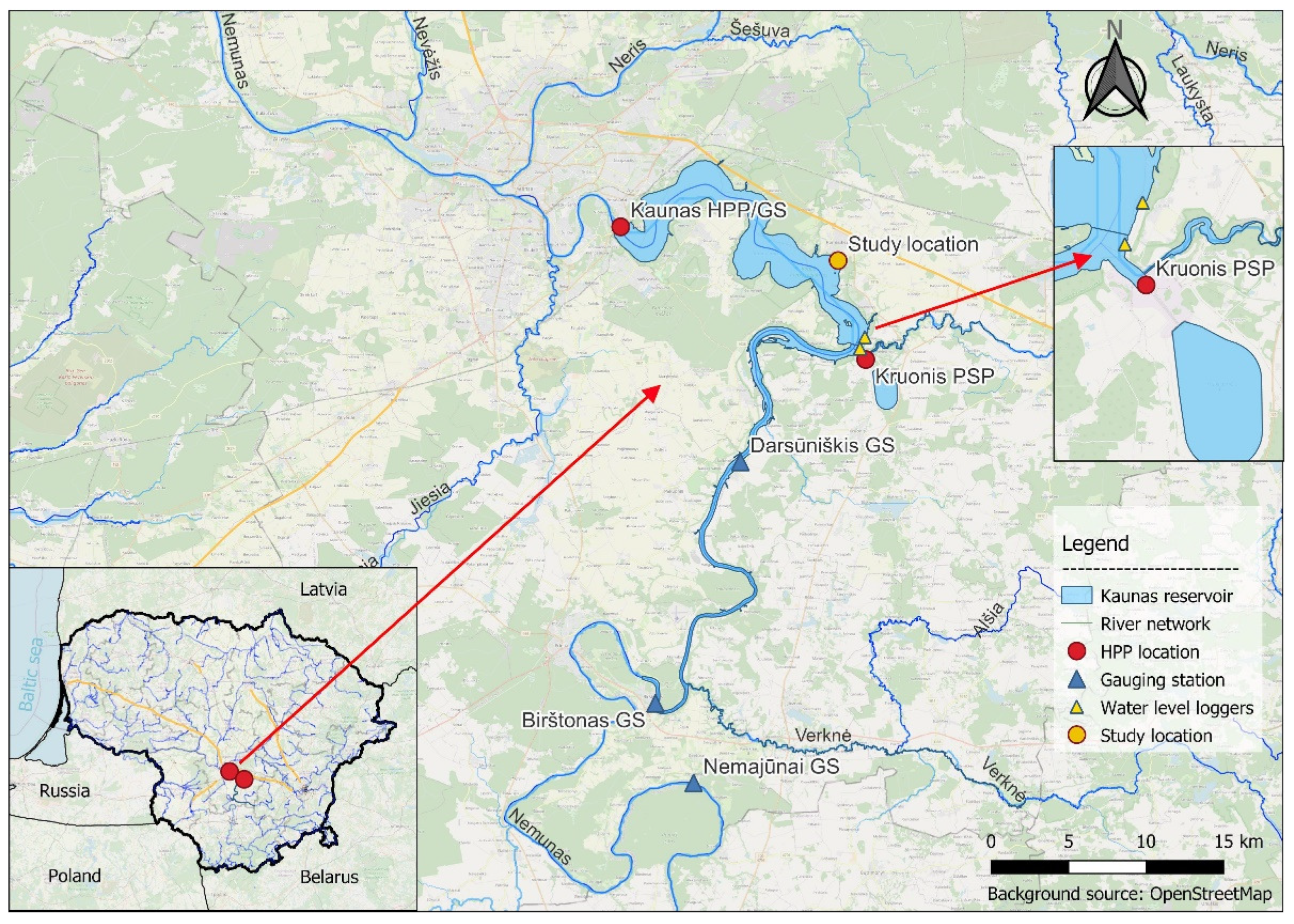
The study area was selected at the northeastern shore of the reservoir in between the Kaunas HPP and Kruonis PSP. It is one of the main spawning sites for perch, common roach, and common bream [17]. The size of the selected area was about 5 ha and contained several potential fish spawning sites. The bottom of the reservoir in this area was very shallow and gently sloping. The study area contained shallow sandy beaches, steep banks covered with land vegetation, and several areas containing aquatic macrophytes (reeds and bulrush) (Figure 1).

2.2. Bathymetric Survey

Field survey missions were conducted on 4–5 March and 8–9 June 2021. Elevation measurements of the bottom of the reservoir were collected. During the winter, the priority was to collect data in the part of reservoir with the thick vegetation of reeds and bulrush—the typical spawning site for many species of fish. March 2021 was very cold, and the data were collected from the ice, making it much easier than it would have been during a warmer period. The water depth was measured using mechanical devices for accurate readings. The advantage of this kind of survey is that it was possible to collect accurate data in places where devices based on echo-sounding (sonars) cannot operate—in the shallow waters containing aquatic macrophytes. The water depth was measured with a water measuring pole with markings every centimeter and a plate on the bottom to prevent it from sinking into the sediment. A special iron weight attached to a graduated lead-line was also used to verify the results. The principles of limnological reconnaissance and the tools that are used for water depth measurements are described in [28,29].

Data were collected in the 5 profiles (straight lines) that were perpendicular to the shoreline and parallel to each other. The profiles were 25 m apart and covered about 1.2 ha of the research area. The ice was drilled, the water measuring pole was carefully placed in the holes, and the depth was visually inspected according to the markings and the water level. Water depth measurements were collected at 1, 3, 5, 10, 15, 25, 35, 50, 75 and 100 m distance, starting from the shoreline. Measured places are presented as red circles with crosses (Figure 2).

The area more likely to be affected by the change in water level in the reservoir (in the littoral zone) was surveyed in more detail than the areas with less relevance. The exact position of each measurement was collected with the Trimble R6 GNSS receiver. The point positioning accuracy using LitPOS RTK is 3–5 cm in the horizontal axis and 5–8 cm in the vertical axis. The water level elevation was measured in 18 places, to eliminate systematic errors and the average of these measurements was set as the reference plane (0.0 m).

Elevation profiles according to the water depth measurements were drawn using AutoCAD 2021 software. The vertical scale of the profiles was 1:10 and the horizontal scale was 1:1000. Measured water depth was plotted according to the reference plane (H = 0.0 m in the drawings) for easier interpretation. The actual elevation of the reference plane was 43.85 m a.s.l. The upper and lower limits of the allowed water level during the fish spawning period are marked in the drawings.

The second part of the study was conducted on 8–9 June 2021. The elevation of the bottom of the reservoir, banks, and the terrain of the study area was measured using a geodetic-grade GNSS receiver (Trimble R6) attached to a 2 m pole. The water depth in the research areas was too shallow for echo-sounding but allowed us to measure the bottom of the reservoir using the GNSS receiver attached to a pole. Additionally, over 1000 points were measured in the study area, which appear as yellow dots (Figure 2). These measurements were used to generate the digital elevation model (DEM) of the research area.

The currently available dataset of the bathymetry of the Kaunas HPP reservoir was compared to the measured data using GIS and CAD tools. For the comparison, a currently availableDEM with a spatial resolution of 1 m was used, which was created by the Lithuanian Inland Waterways Authority (LIWA). Elevations in the exact same points as the measured data were determined in the QGIS software and plotted according to the same reference plane using AutoCAD software.

2.3. Analysis of the Digital Elevation Models

Five different digital elevation models were created using all points that were measured during the field surveys. The DEMs were created as raster files with ArcGIS Pro software, using different interpolation methods. Details of the interpolation process and results are discussed further in Section 3. These techniques are part of the Spatial Analyst tool kit based on a GIS environment and described in detail in ArcGIS Pro geoprocessing tool reference documentation [30]. IDW (inverse distance weighted), Kriging, Natural Neighbor, and Topo to Raster interpolation tools were used to create the DEM as raster files, where each pixel represents the elevation of the Kaunas HPP reservoir bottom. Ground control points (GCPs) were established at the locations where the field measurements were collected. At the same control points, the elevations were determined from the generated elevation models. This step was completed by converting the points into 3D vector features, sampling the generated DEMs, and calculating their elevation geometry. It allowed us to compare the interpolated data of each DEM with the actual measured data.

Visual analysis and statistical parameters were adopted for comparative evaluation of the interpolated surfaces. For the visual analysis, digital elevation models were analyzed for any discrepancies using the Terrain profile tool in QGIS. Elevation profiles were visually inspected and compared to measured data. Mathematical analysis was conducted by calculating deviations of the interpolated values from the corresponding measured data at GCPs in terms of root mean square error (RMSE) values. This methodology has been discussed by other authors [31,32,33]. It was also important to know how the interpolated elevation values deviated from the measured data. The mean, minimum, maximum and the standard deviation coefficient of errors were calculated. These parameters allowed us to estimate whether there were discrepancies that were overlooked by the RMSE.

A statistical analysis was conducted with two datasets—the first one included all measured points (1052) and the second included the points that only covered the allowed water level fluctuation range in the reservoir (43.4–44.5 m a.s.l). This dataset contained 531 control points. This approach allowed us to analyze the overall accuracy of the generated digital elevation models, but at the same time put more emphasis on the area that is the most important for the study.

For further examination of the accuracy of each interpolation method, the scatterplots between the interpolated and observed values were drawn and the determination and correlation coefficients were calculated. The higher the matching degree between the interpolated and observed values, the closer the correlation coefficient should be to 1 [34].

To visually compare the performances of the four interpolation methods, the error distributions of different interpolation methods were presented as box plots using MATLAB. This technique is commonly used for various applications. It was used by [34] for a comparison of the performance of different interpolation methods in replicating rainfall magnitudes under different climatic conditions [33].

2.4. Dewatering Area Analysis during Drawdown Operations

After the most representative DEM of the investigated potential spawning site and the surrounding area was selected, the data were fed into a binary-thresholding step where the DEM was intersected with the water level data. Whenever the elevation values of the DEM were lower than or equal to the set WL value, outcoming raster image values were set to 1; otherwise, they were set to 0. These raster data files were converted into vector data, which represented submerged areas (where the terrain elevation was under the set water level) and dry areas where the terrain was above the set water level. Submerged and dewatered areas were calculated throughout the water level fluctuation range that covered the entire HPP operating regime (43.5–44.4 m a.s.l.) with an additional 10 cm outside of the range for the additional data input to create a morphometric curve. Calculations were carried out from 43.4 to 44.5 m a.s.l. at intervals of 0.1 m. For the range of water levels that are allowed during the fish spawning period (43.7 to 44.0 m a.s.l.), the interval for the calculations was 0.05 m.

The researched potential fish spawning site was traced out as a polygon from the ultra-high-resolution orthographic image (with the ground sampling distance under 2 cm). Using the GIS tool, a polygon of the entire area of the potential fish spawning site was intersected with the polygons that represent submerged areas during various water levels in the reservoir. This procedure allowed us to track submerged area changes in the spawning site and determine the dewatering areas.

A curve of the submerged area of the spawning site was plotted as a function of water level in the reservoir.

2.5. Water Level Fluctuation and Dewatering Areas Analysis in the Selected Site

Two water level loggers were set nearside the Kruonis PSP. They were set 300 m and 1 km away from the water intake and outlet (Figure 3). Water level data were collected from May 2021 to May 2022. Additionally, data from the Kaunas HPP, Kruonis, Birštonas, and Nemajūnai gauging stations were used alongside the sensor data to analyze the water level fluctuations in the reservoir and how they were influenced by the operation of the hydropower plants. The mentioned gauging stations collected hourly WL data, and their locations are presented in Figure 1.

For this study, research-grade water level loggers were used (Onset HOBO U20L-04) that feature 0.1% measurement accuracy (typical error: ±0.1% FS, 0.4 cm). They use ceramic pressure sensors to continuously measure the water level and temperature. The time step of the recordings was set to 30 min, and data were collected for a year. The water level elevation was measured with a Trimble R6 GNSS receiver to reference the measured water depth data to the actual water level elevation.

The four turbines of the Kruonis PSP are able to work in power generation and water pumping modes. In power generation mode, each turbine has the power output of 225 MW and a discharge rate of 226 m³/s at full capacity. In water pumping mode, each turbine outputs at 217 MW and 189 m³/s. The effective volume of the upper reservoir of the Kruonis PSP is 41 million m³; for comparison, it is about 9% of the total volume of the entire Kaunas HPP reservoir and the stored capacity is about 11.3 GWh. Operation of the Kruonis PSP can dislocate a considerable amount of water. The Kruonis PSP has four places for additional turbines in reserve. A fifth turbine is currently in the design stage and will be installed in the near future.

Hydrographs for each month were plotted and analyzed using Microsoft Excel to study the water level fluctuations. They were analyzed according to data from the installed sensors and gauging stations mentioned earlier. The highest, the lowest, and average daily water levels were detected (for every 24 h period), and the daily WL drawdowns were calculated.

For further analysis, two time periods with very consistent inflow to the reservoir were selected to study the water level fluctuations when the power plants are operating. The first period was 13–20 June 2021. During that period, HPP operation was constricted (daily drawdown limit—0.2 m) because of the fish spawning period. The inflow data were taken from the Nemajūnai GS, where the water flow is not affected by the hydropower plants. During the first time period, the inflow to the reservoir was very constant, 166 m³/s on average. The second period was 9–16 November 2021. During that time, the HPPs were operating under a less restrictive regime, with an allowed daily drawdown of 0.4 m. The inflow to the reservoir was also very constant, 180 m³/s on average.

Furthermore, submerged area changes in the selected potential fish spawning site were analyzed in the context of time. Submerged areas in the spawning site were determined from the morphometric curve (see Section 2.4) according to average daily water levels in the site. Analysis was conducted for the time period starting 1 April 2021 to the end of the year.

3. Results

3.1. Elevation Profiles of the Litoral Zones

The measured water depth data and the data from the digital elevation model provided by the LIWA were plotted as the elevation profiles (Figure 3).

Figure 3. Elevation profiles of the littoral zones of the reservoir.

Figure 3. Elevation profiles of the littoral zones of the reservoir.

The elevation profiles revealed large differences between the measured and DEM data in the foreshore areas of the reservoir. The DEM is a combination of two data sources—LiDAR data of the terrain and echosounder data of the bottom of the reservoir. The nearshore of the reservoir was not explored because it was impossible to collect data in shallow areas using sonar, and the LiDAR data were available only for the terrain above the water. Linear interpolation was used to merge the two datasets.

Judging from the elevation profiles, the current DEM provided by the LIWA has limitations. It is fine for navigation in the reservoir, but it cannot be used to study shallow parts of the reservoir.

3.2. Analysis of the Generated Digital Elevation Models

Mathematical analysis of digital elevation models created from measured water depth data in the littoral zone was an important part of the study. The quality of generated models directly corresponded to the accuracy of the calculated dewatering areas in the fish spawning sites. The generated DEMs were compared according to the RMSE between the interpolated and measured data and the standard deviation of the errors between the corresponding measured and predicted points. Additionally, the determination and correlation coefficients are shown in

Table 2. Results of the statistical analysis of the generated digital elevation models.

	IDW	Kriging	Natural Neighbor	Topo to Raster
All points (1052)
RMSE, m	0.029	0.028	0.033	0.045
Standard deviation, m	0.027	0.026	0.029	0.040
Determination coefficient	0.998	0.998	0.997	0.995
Correlation coefficient	0.999	0.999	0.999	0.998
43.4–44.5 m a.s.l. (531 points)
RMSE, m	0.038	0.036	0.039	0.055
Standard deviation, m	0.035	0.031	0.035	0.048
Determination coefficient	0.989	0.991	0.989	0.977
Correlation coefficient	0.995	0.995	0.994	0.988

. The methodology of the statistical analysis was described in Section 2.3.

Statistical analysis indicated that all models had good accuracy. If we assume up to 0.08 m of vertical measurement error (associated with the accuracy of the GNSS receiver) and the 0.04 m error due to interpolation, our generated DEM is consistent with the highest accuracy of Exclusive Order according to the IHO standards for hydrographic surveys [35]. IDW and Kriging interpolation methods had the lowest values of RMSE and standard deviation of the errors, which meant that they fit the measured data the best, and the determination and correlations coefficients showed a very high correlation between the interpolated and measured values. The correlation was almost linear, as was expected. The RMSE and standard deviation were worse for the second dataset, which contained only the points with an elevation between 43.4–44.5 m a.s.l. The elevation changes were very gradual farther from the banks of the reservoir (Figure 3). In contrast, the elevation changes were much steeper in the range of the second dataset, which represented an area closer to the shore. The banks of the reservoir are quite steep, and this was where the interpolation errors were the highest. The accuracy of the models in these conditions was more important as it corresponded to the areas affected by the WL drawdowns. Formulas that are used for interpolation can have a bigger impact on the accuracy in the areas with steeper elevation changes, as demonstrated by the increased RMSE of all interpolation methods.

To evaluate the digital elevation models further, errors between the measured and interpolated values of the second dataset were plotted as box plots to offer a visual representation of the datasets (Figure 4).

The red line symbolizes the median value of the errors. It was essentially a zero for all methods. More interestingly, the upper and lower edges of the blue rectangle (i.e., box) were defined as the 75th and 25th percentile of the dataset, and the upper and the lower whiskers (black lines) were drawn to the 90th and 10th percentiles. This meant that 50% of the values of the dataset were in the range of the blue box and 80% of the values were between the black lines. Looking at the figure, the boxes of all methods are very small, which means that 50% of the values in the DEM were within 1 cm of the measured data. Whiskers of the IDW were close to zero, which meant that 80% of the data errors were within 1 cm of the measured data. Whiskers of the Kriging interpolation indicated that 80% of the data were within 1.7 cm of the measured values. Topo to Raster performed the worst—80% of the generated values were within ±2.5 cm of the measured data. The IDW performed the best, but the outliers (the red crosses that represent the remaining 20% of the values) emphasized the problem with the IDW method. Outliers are the furthest points from the median—the highest errors. The outliers of the IDW were distributed wider from the median compared to the Kriging. The maximum errors of the IDW were 0.24 and −0.39 m. The highest errors of the Kriging were 0.23 and −0.21 m. Disregarding the extreme values, the outliers were grouped more densely around the whiskers for the Kriging method, which meant it was more accurate in the areas where the models were struggling.

Elevation profiles in various places were plotted for each digital elevation model. During the visual inspection it was noticed that the banks of the reservoir, where the elevation changes were the steepest, had the highest difference when comparing the interpolated and measured data. The DEM created with the Kriging method showed the best results in those areas, as was expected, from the analysis of the box plots. When the elevation changes were gradual, the IDW method was the most accurate, but all interpolation methods gave good results. The Kriging method performed better in the areas with steep elevation changes, compared to the IDW. Similar results have been observed by other authors [31,36].

The digital elevation model created with the Kriging interpolation method was chosen for the analysis of dewatering areas.

3.3. Dewatered Areas during Drawdown Operations

After the binary-thresholding step, which was discussed in Section 2.4, the polygons representing the submerged and dewatered areas in the spawning site at certain water levels were determined (Figure 5).

These polygons visualize how the shoreline changed when the water level fluctuated and allowed us to calculate the dewatered areas. Using QGIS, the area of each polygon was calculated and the morphometric curve as a function of the submerged area in the spawning site to the water level was plotted using AutoCAD (Figure 6).

The selected potential fish spawning site was fully submerged when the water level reached 44.4 m a.s.l. The banks of the reservoir are steep. When the water levels rose to 44.2 m a.s.l. and above, the area of the spawning site did not change much because the site was mostly submerged. The curve flattens from 43.85 m a.s.l. and below, which means that the bottom of the reservoir was shallow with a low slope. Water level fluctuations in this range were the most impactful for the spawning site because small changes in water level resulted in large dewatered areas. The water level allowed in the reservoir during the spawning period ranged from 44.0 to 43.7 m a.s.l. At these water levels, about 89% and 42.6% of the spawning site were submerged. There was a big decrease in submerged area (from 1148 to 712 m²) when the water level changed from 43.8 to 43.7 m a.s.l. When the water level decreased from 44.0 to 43.7 m a.s.l, the total drawdown area in the spawning site was 772 m². The water level change from 43.8 to 43.7 m a.s.l. accounted for a large part of it—nearly 60% (the dewatered area was 436 m²).

3.4. Analysis of the Water Level Sensor Data

According to the water level data, there were several instances when the limit of allowed drawdown was reached during the fish spawning period in 2021 (from 1 April to 30 June). The maximum and minimum daily water levels and the drawdown height (H) are presented in

Table 3. Instances when the drawdown height limits were reached during the fish spawning period of 2021.

Location	Parameter	April	May		June
		23	6	20	13	20	23	28
Kaunas HPP	Max WL elev., m	43.93	43.98	43.92	43.95	43.94	43.93	43.92
	Min WL elev., m	43.73	43.8	43.75	43.72	43.76	43.78	43.72
	Drawdown H, m	0.2	0.18	0.17	0.23	0.18	0.15	0.20
WL logger at Kruonis PSP	Max WL elev., m	-	43.98	44.06	43.88	44.00	44.03	43.96
	Min WL elev., m	-	43.76	43.85	43.70	43.80	43.83	43.75
	Drawdown H, m	-	0.22	0.21	0.18	0.20	0.20	0.21
Darsūniškis GS	Max WL elev., m	44.05	44.08	44.06	44.05	44.06	44.12	44.06
	Min WL elev., m	43.85	43.92	43.87	43.85	43.90	43.91	43.86
	Drawdown H, m	0.20	0.16	0.19	0.20	0.16	0.21	0.20
Birštonas GS	Max WL elev., m	44.18	44.21	44.23	44.15	44.15	44.16	-
	Min WL elev., m	44.00	44.07	44.06	44.02	44.10	44.13	-
	Drawdown H, m	0.18	0.14	0.17	0.13	0.05	0.03	-

.

Hydropower plants operate on a restrictive peaking mode without breaking the operation rules. Analysis of the water level logger data indicated that the drawdowns right beside the Kruonis PSP were bigger than in the rest of the reservoir owing to the large quantity of water being released or pumped out. The effect was localized, and the drawdowns decreased in the adjacent gauging stations because of the backwater. In the same matter, on 13 June, the daily drawdown was higher than permitted at the Kaunas HP, but in the rest of the reservoir, both the daily drawdown and the water level ranges were within the limits.

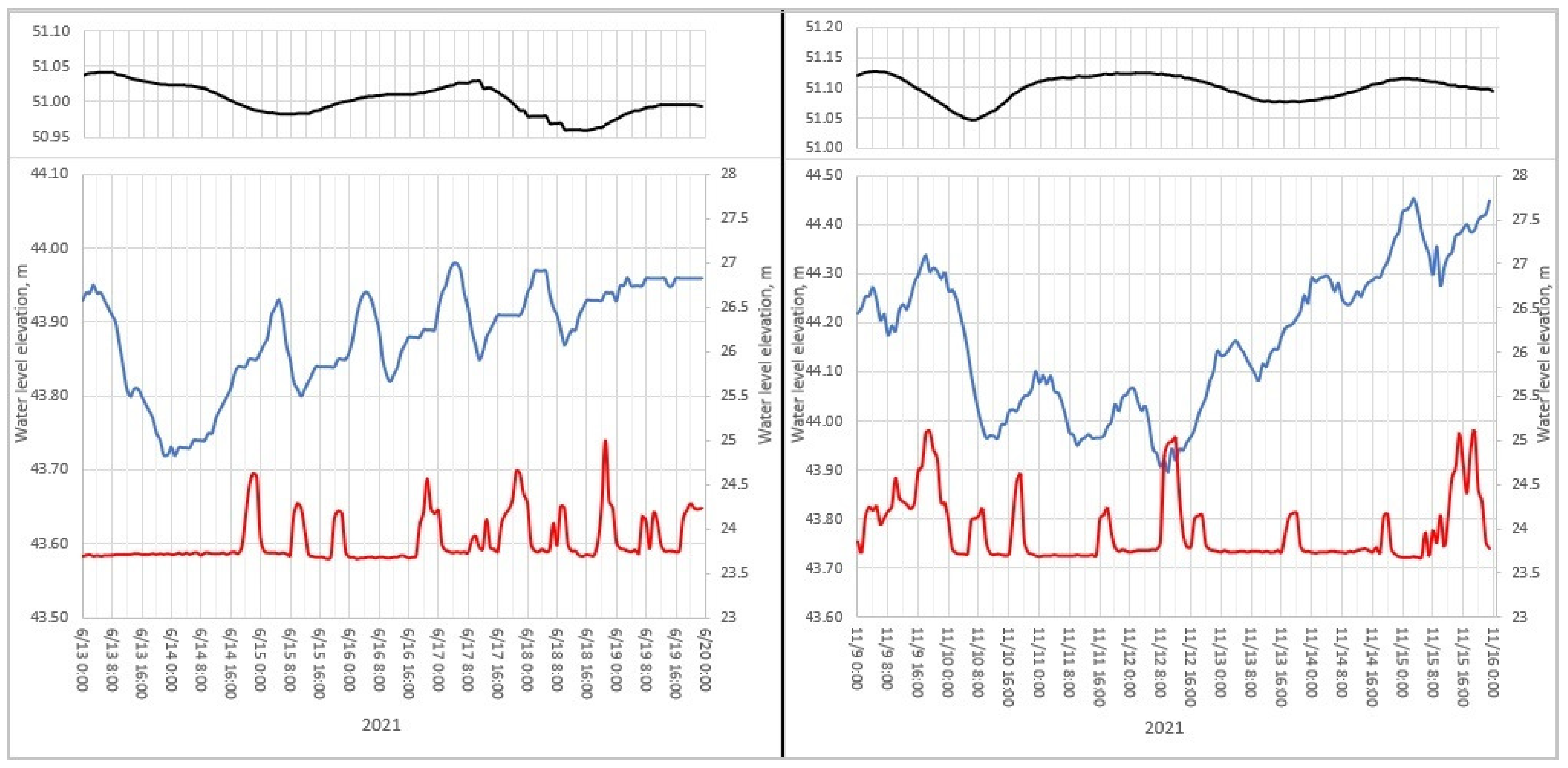
Hydrographs were plotted to better understand how the peaking operation of HPPs influenced the water level fluctuations in the reservoir (Figure 7).

On both occasions, the water level at the Nemajūnai GS (black line) was very steady, and fluctuations were under 10 cm throughout the selected time periods. The inflow to the reservoir was constant and did not cause any considerable water level fluctuation in the reservoir. There is no significant inflow to the Nemunas River downstream from the Nemajūnai GS. The hydrographs show at what time the Kaunas HPP started and stopped the turbines based on the water level data of the Nemunas River downstream from the Kaunas HPP (red line on the secondary axis). The most significant water level decreases occurred at night (blue line), usually from 4 am to 8 am when the water from the Kaunas HPP reservoir was being pumped to the upper basin of the Kruonis PSP. After 8 am, the Kruonis PSP began slowly releasing water back into the Kaunas HPP reservoir, and the Kaunas HPP started the turbines as well. When both power plants were working together, the water level in the reservoir rose slowly. Typically, a step in the uprise of the water level was detected when the Kaunas HPP was operating. After the Kaunas HPP turbines were turned off, the water level peaked until the Kruonis PSP stopped operating. In the summer, the Kaunas HPP usually produces electricity in the evenings from about 7 pm to 12 am. In the autumn–winter, the Kaunas HPP usually works twice a day—in the morning from about 8 am to 12 pm and in the evening from 5 pm to about 9 pm.

The hydrographs show the water level fluctuations in the reservoir. The resulting dewatering areas in the potential fish spawning site are presented in Figure 8.

This graph shows how the dewatered area changed in the selected potential fish spawning site from 1 April 2021 to the end of the year. The water level in the reservoir did not fluctuate much during the restricted period, and on average, 84% of the spawning site was submerged. The drawdown area changed from 167 to 444 m². During the normal operating regime, the water level fluctuations increased. With the wider permitted water level range (43.5 to 44.4 m a.s.l. instead of 43.7 to 44.0 m a.s.l.), the drawdown area changes were more substantial. With the higher permitted drawdowns, up to 75% of the spawning site area was dewatering. The water level in the reservoir is usually kept higher to maintain enough water for bigger drawdowns. After the restricted period, the drawdown area changed from 0 (fully flooded) to 1092 m² (out of a total 1671 m²).

4. Discussion

Comprehensive research on the dewatering areas during drawdown operations and water level fluctuations in the reservoir indicated that large multipurpose reservoirs in lowland countries are susceptible to various ecological problems owing to their morphology, which was discussed in the introduction. Accurate data of the most vulnerable littoral areas are crucial for the optimal operation of the reservoir.

Analysis of previous studies [17,18,19,20,21,22,23,24] and our detailed study provided valuable information on how the operation of two large hydropower plants affects the water levels and dewatering areas in the reservoir. A bathymetric survey showed that the currently used DEM does not accurately represent the shallow littoral zone (Figure 3) owing to the shortcomings of echo-sounding and cannot be used to determine the drawdowns in the reservoir. Accurate bathymetric data is needed for the shallow nearshore areas. Traditional bathymetric surveys provided reliable data about the selected area, but the application is limited as conducting this kind of survey is hard in difficult conditions. For this reason, alternative surveying methods were implemented, and the same location was used as the testing site. The data and the analysis of this research were necessary for the following research and were used as the reference.

A selected digital elevation model was used to determine the dewatering areas in the investigated potential fish spawning site according to different water levels in the reservoir. A similar technique was used for shoreline detection in the coastal area [37]. The article discussed algorithms that have been used to substantiate and extract the shoreline from the DEM created from LiDAR data and aerial images. There have been other approaches using satellite data [38,39,40]. In this instance, the DEM was created from bathymetric measurements using conventional methods. LiDAR data were also available, but the investigated areas affected by the water level fluctuations and containing water macrophytes were better represented by the field measurement data. Shoreline detection using satellite images was also a valuable option, but better suited to studying areas with gradual changes (e.g., from erosion) or areas affected by big changes (e.g., during floods). Resolution of most satellite images is not very high, and it is not very useful to track small changes, as in our case.

The results of this survey can be used in different ways. The generated morphometric curve (Figure 6) proved to be very useful as it allowed us to track the dewatering area changes over time (Figure 8) and could be used to quickly evaluate how certain water level changes can affect the spawning sites in shallow areas. This was a unique approach, showcasing the WL fluctuations from a different angle. It enabled us to track the actual measurable changes occurring in vulnerable areas in the context of HPP operations. It can be used for different purposes, such as evaluating the daily operation schedule or altering the operation regime of the powerplants.

Our analysis of water level data provided interesting results. During the fish spawning season, the daily drawdown was usually 10–15 cm (Figure 7). During the normal operating regime (cold period of the year), WL drawdowns were often quite similar, only sometimes reaching a WL change higher than 20–30 cm, and occasionally it was in the 40 cm range. The biggest difference was in the water level fluctuations. During the restricted operating regime, the water level in the reservoir was kept very steady between 44.0 and 43.8 m a.s.l., sometimes dipping to 43.7 m a.s.l., which was still within allowed limits. In the normal operating regime, daily drawdowns were not that much bigger, but the water level in the reservoir fluctuated on a wider scale, which allowed for better usage of reservoir storage for hydropower. The water level was usually kept higher, allowing for bigger drawdowns when there was higher demand for electricity (Figure 7).

Considering how these two different regimes affected the dewatered areas (Figure 8), it was noticeable that in the normal operating regime, the dewatered areas were much larger. These water level changes did not happen suddenly. For example, looking at the drawdown that occurred on 9 November, it took about 16 h for the WL to lower 0.37 m, which was close to the maximum allowed limit (0.4 m). To give more context, water level elevation change rates were analyzed for June 2021 and November 2021. In June (power plants were operating in restricted regime), the maximum drawdown rate in the reservoir was 0.04 m/h at Kaunas HPP, 0.08 m/h at Kruonis PSP and 0.06 m/h at Darsūniškis GS. The maximum refill rates were as follows: 0.05 m/h at Kaunas HPP, 0.08 m/h at Kruonis PSP and 0.07 m/h at Darsūniškis GS. In November (power plants were operating in normal regime), the maximum drawdown rate in the reservoir was 0.05 m/h at Kaunas HPP, 0.13 m/h at Kruonis PSP and 0.07 m/h at Darsūniškis GS. The maximum refill rates were as follows: 0.05 m/h at Kaunas HPP, 0.07 m/h at Kruonis PSP and 0.08 m/h at Darsūniškis GS. Even though the dewatered areas were significant during the cold period of the year, the drawdown rate was low, close to the natural fluctuations in the rivers. Numerous previous studies have explored the impact of water level fluctuations and ramping speed on the stranding of juvenile fish but have generally only addressed the effects on salmonid species [41,42,43]. These studies focused on rivers with an artificially regulated regime usually caused by hydropower plants that operate in a peaking regime. Comparatively little is known about effects on non-salmonid species as discussed in other studies [44]. Moreover, the ability of fish to resist stranding is dependent on life stage, the swimming ability of the individual, size, muscle function, and swimming biomechanics [45]. These studies were not directly applicable to a reservoir, and the evaluation of the drawdowns is not a simple question. Nevertheless, some conclusions can be drawn from the studies mentioned above. They found that water level decrease rates slower than 10 cm/h have a low probability of stranding fish. Drawdown rates in the reservoir are very low, compared to the ramping rates in the rivers downstream from the HPP. Current drawdown rates in the Kaunas HPP reservoir do not exceed 2 cm/h, which indicates that drawdowns could potentially be increased (excluding the spawning period). Additional research must be conducted using a similar methodology to the studies discussed above, but it must be tailored to the conditions of the reservoir and additional factors must be evaluated. A relevant review of the ecological impacts of winter water level drawdowns on lake littoral zones [46] showcased other factors that must be considered when evaluating regulated lakes and river reservoirs.

Since it pertains to a multipurpose reservoir, this information can be used to adjust the operating regime, allowing bigger drawdowns in the cold period of the year when there will be less impact on the environment and energy consumption increases but keeping the fish and water birds protected during the spawning period. Such decisions can increase power generation, but reliable and accurate bathymetry of the littoral zones is needed for better evaluation.

5. Conclusions

The research area of about 5 ha was very small compared to the total area of the reservoir, which is 63.5 km² at the normal water level. Different spawning sites will have different morphologies, and these results cannot be applied to the entire reservoir. The purpose of this research was to gather information and fill the knowledge gaps, as there were very few studies on the matter in lowland countries and explore the possibilities of utilizing different surveying methods to assist in improving usage of reservoir storage while increasing power generation. The findings of this study provide some insights into how the operation of the hydropower plants causes water level fluctuations in the reservoir and what areas are dewatering during drawdown operations in the very shallow nearshore areas with gently sloping banks. This study compares different surveying and data analysis techniques that can be adopted for the following studies.

The results of this study will be used as a reference in ongoing research in which the same area is monitored using remote surveying techniques and analyzed using photogrammetry and machine learning [47]. Research outcomes can be applied to larger territories, even to the entire reservoir to a degree.