Article

Fast Quasi-Static Time-Series Simulation for Accurate PV Inverter Semiconductor Fatigue Analysis with a Long-Term Solar Profile †

1
Department of Electrical Engineering, The Pennsylvania State University, University Park, PA 16802, USA
2
Department of Electrical Engineering and Computer Science, The University of Tennessee, Knoxville, TN 37996, USA
3
Oak Ridge National Laboratory, Oak Ridge, TN 37831, USA
4
Pacific Northwest National Laboratory, Richland, WA 99354, USA
5
National Renewable Energy Laboratory, Golden, CO 80401, USA
*
Author to whom correspondence should be addressed.
This paper is an extended version of our paper published in 2021 IEEE Power & Energy Society General Meeting, Washington, DC, USA, 26–29 July 2021; pp. 1–5.
Submission received: 13 October 2022 / Revised: 19 November 2022 / Accepted: 25 November 2022 / Published: 1 December 2022

Abstract

:
Power system simulations with long-term data typically have large time steps, varying from one second to a few minutes. However, for PV inverter semiconductors in grid-connected applications, the minimum thermal stress cycle occurs over the fundamental grid frequency (50 or 60 Hz). This requires the time step of the fatigue simulation to be approximately 100 μs. This small time step requires long computation times to process yearly power production profiles. In this paper, we propose a fast fatigue simulation for inverter semiconductors using the quasi-static time-series simulation concept. The proposed simulation calculates the steady state of the semiconductor junction temperature using a fast Fourier transform. The small thermal cycling during a switching period and even over the fundamental waveform is disregarded to further accelerate the simulation speed. The resulting time step of the fatigue simulation is 15 min, which is consistent with the solar dataset. The error of the proposed simulation is 0.16% compared to the fatigue simulation results using the complete thermal stress profile. The error of the proposed method is significantly less than the conventional averaged thermal profile. A PV inverter that responds to a transactive energy system is simulated to demonstrate the use of the proposed fatigue simulation. The proposed simulation has the potential to cosimulate with system-level simulation tools that also adopt the quasi-static time-series concept.

1. Introduction

Solar photovoltaic (PV) integration requires power electronic inverters to interface with 50/60 Hz power systems. Many studies have reported that powered electronic devices have shorter lifetimes compared to their associated PV panels [1,2]. For example, in a PV system, the lifetime of PV panels is normally warrantied at 20–30 years, whereas the PV inverter lifetime is usually limited to less than 15 years [1]. Semiconductors are among the most vulnerable components that lead to inverter failure [3], and they are sensitive to temperature [4,5,6]. High operating temperature and large thermal cycling are the two main causes of rapid semiconductor aging [5,6].
To extend the lifetime of PV inverters, many methods have been tested in simulation-based aging analysis to evaluate their performance. Scheuermann et al. [7] presented a lifetime model to predict the accumulated fatigue of semiconductor bond wires. Similar lifetime models were used in [6,8,9,10,11,12,13]. This lifetime model of semiconductors has the potential to be extended to grid-level simulations and incorporated into reliability studies. The lifetime model proposed in [7] uses a limited dataset, which may result in marginal accuracy for long-term aging evaluation. Other lifetime models that are widely used in inverter reliability evaluation include those presented in [6] and [14]. The derivation of such lifetime models typically involves accelerated tests and limited datasets. Once the expected lifetime of a semiconductor is derived, the result can be further extended to a proper stochastic distribution, and a Monte Carlo simulation can be conducted to determine the lifetime expectation for the entire inverter system. Some researchers have adopted a stochastic process, such as Monte Carlo simulation, to study inverter reliability [15,16,17,18]. Some studies have suggested replacing the semiconductor aging model with indirect measurements, such as IGBT turn-on losses [19] and case temperature [20], to estimate the health of the semiconductor.
Simulation-based aging analysis typically involves three steps [21,22,23,24,25]: (1) an electrothermal model to calculate the semiconductor junction temperature, (2) a rainflow-counting algorithm to assess the temperature profile, and (3) a semiconductor aging model to estimate the degradation. Some simulation-based aging analyses also include the Monte Carlo simulation to further interpret the result of the semiconductor aging model as part of a stochastic process.
Among the three steps, the junction temperature calculation and rainflow-counting (thermal cycles) can be time-consuming because the junction temperature profile is strongly related to the converter switching actions. The corresponding time step of the junction temperature calculation is approximately 100 μs, owing to the fast switching frequency (10 to 100 kHz) of the inverter if the conventional Euler–Maruyama method is applied to the simulation [26].
To accelerate the fatigue simulation, multiple solutions have been proposed in the literature. To accelerate the junction temperature calculation, a lumped thermal network is normally used for long-term thermal stress analysis of PV inverters, owing to its low computational burden [6,14,22,27,28,29,30]. Conventionally, a lumped thermal network is either based on (1) the full-order thermal model [28,29,30], which includes all the transient thermal impedances; (2) the steady-state lumped thermal model [31,32,33], which only considers the thermal resistance; or (3) the reduced-order lumped thermal model [22], which keeps the thermal capacitances with a larger time constant so that the thermal dynamics can be partially captured. Among the three major conventional methods, the full-order thermal model provides the most accurate thermal stress modeling under dynamic conditions; however, it requires a much higher computational effort during simulation compared to the steady-state thermal model and the reduced-order thermal model. In addition, several look-up-table-based methods have been proposed to eliminate the junction temperature calculation [15,23,24].
Regardless of the thermal model that a fatigue simulation may choose, most fatigue simulations need to reduce the junction temperature profile to accelerate the computational speed of rainflow counting. The most common approach to reduce the thermal profile is to average the junction temperature every fundamental cycle (50 or 60 Hz) [6,22,27,28,29,30,31,32,33,34,35,36]. However, this method may result in the loss the peak and valley information when averaging the junction temperature. Most existing acceleration methods focus on the junction temperature calculation. Few publications in the literature have reported acceleration methods for calculating reliability by focusing on rainflow counting. The current research gap of rainflow counting acceleration can be summarized as follows:
  • The acceleration of rainflow counting is generally required when conducting fatigue simulations with a long-term profile. The current approaches typically eliminate all high-frequency thermal cycling by averaging the junction temperature every fundamental cycle, which may eliminate the actual tensile peaks and compressive valleys. However, the actual junction temperature tensile peaks and compressive valleys are important data needed to conduct aging analysis. To restore junction temperature peaks and valleys, a full thermal profile must be obtained, which may significantly increase the computing time of rainflow counting.
In this paper, we leverage the quasi-static time series concept to simulate the fatigue of inverter semiconductors over long periods of time. Simulation-based aging analysis for semiconductors can be incorporated with power system simulations so that a specific grid code can be tested for its aging effect on grid-connected inverters. Power system simulations typically adopt a quasi-static time-series (QSTS) approach to evaluate a system with data ranging from several days to several years [37,38]. QSTS simulations provide a good representation of time-varying characteristics in grid objects that incorporate various control systems, such as voltage regulators and shunt capacitors [39].
In this paper, we propose a fast semiconductor fatigue simulation approach that can be extended to QSTS simulations. The proposed approach incorporates the PV inverter solar irradiance and load profiles as the input and estimates the remaining lifetime of the inverter semiconductors as the output. The proposed approach uses fast Fourier transform (FFT) to calculate the semiconductor junction temperature so that the static junction temperature calculation can be accelerated compared with a Euler–Maruyama-based electrothermal simulation. In addition, small thermal cycling during switching and the fundamental frequency are neglected to further accelerate the rainflow counting. Compared with the averaging methods that are commonly used to disregard the fundamental thermal cycling, the proposed method keeps the actual junction temperature peaks and valleys while accelerating the computation speed. A 7-day simulation and a 2-year simulation are provided to evaluate the proposed fatigue simulation. The computation speed and accuracy of the proposed simulation are benchmarked with a quasi-static time-series fatigue simulation with a complete thermal cycling profile and averaged thermal cycling profile. A PV inverter that responds to a transactive energy system (TES) is simulated to demonstrate the use of the proposed fatigue simulation. The proposed simulation can be incorporated with a semiconductor lifetime model and predict the lifetime expectancy. The major contribution of this paper is summarized as follows:
  • In this paper, we propose a fast computation method for rainflow counting, specifically for the fatigue evaluation of PV inverter semiconductors. The resulting computation time is significantly reduced compared to the conventional complete thermal profile.
  • The proposed thermal profile reduction method removes excessive high-frequency cyclic thermal profiles while maintaining the original peak–valley information. As a result, the accuracy is considerably improved compared to the conventional averaged thermal profile method.
This paper is organized as follows. In Section 2, we present a frequency-domain fast electrothermal simulation method to translate power loss into semiconductor junction temperature. In Section 3, we discuss the proposed fatigue analysis of semiconductors using a rainflow counting algorithm. In Section 4, we discusses the proposed approach in comparison with existing methods. In Section 5, we provides a case study to show the results of the proposed semiconductor fatigue simulation. Finally, Section 6 concludes this paper.
  • Some portions of this paper were presented at the 2021 IEEE PES General Meeting [40]. Section 3, Section 4 and Section 5 are new materials that have been added to the conference paper. The original conference paper includes a case study with a 7-day solar profile, whereas this paper extends the simulation to a 2-year profile to demonstrate its effectiveness for long-term profiling (Section 5). Furthermore, the original conference paper did not include a comparison study, whereas this paper includes a more detailed comparison study of the proposed method with other rainflow counting approaches (Section 4). In addition, in the original conference paper, we did not thoroughly explain the rainflow counting algorithm. This paper includes details of the rainflow counting algorithm that leads to the complete thermal profile, as well as the reduced thermal profile (Section 3).

2. Fast Electrothermal Simulation

Electrothermal simulation is a calculation used to map PV generation to a semiconductor junction temperature profile. To evaluate the junction temperature of a semiconductor, the power loss of the semiconductor needs to be calculated. The power losses modeled by the semiconductor conduction loss and switching loss are the heat source for each semiconductor. The power loss is dissipated into the ambient environment as heat. In this section, we develop a fast Fourier transform (FFT)-based approach to calculate the steady-state junction temperature so that the junction temperature can be used in fatigue analysis.

2.1. Semiconductor Power Loss Formulation

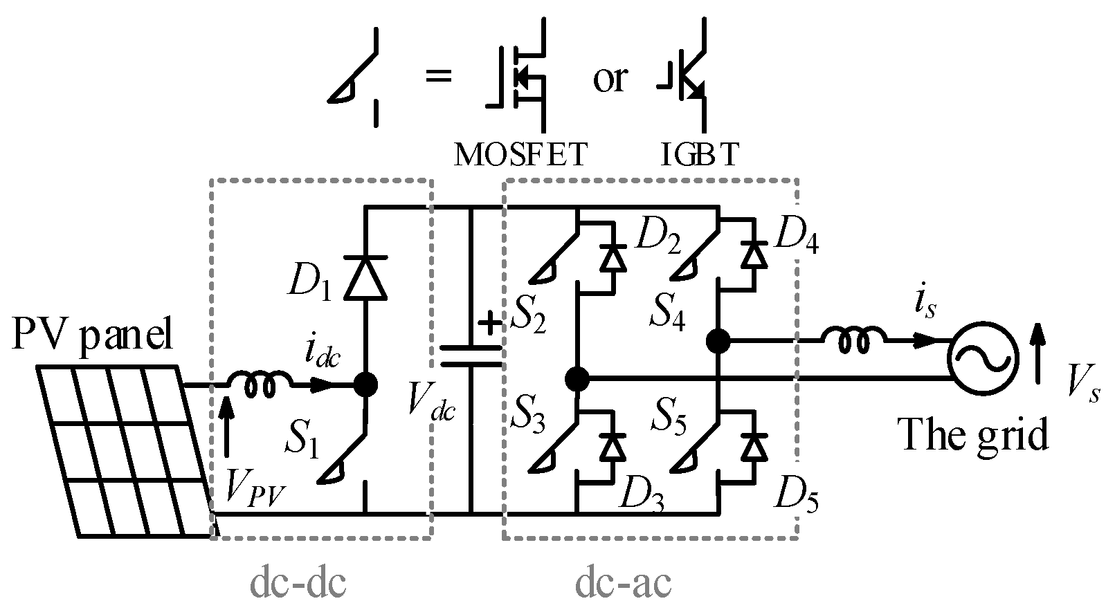
A typical two-stage, single-phase PV inverter topology is shown in Figure 1. The power switches of a PV inverter could be either MOSFETs or IGBTs. The complete semiconductor switching loss and conduction loss for both MOSFET-based and IGBT-based PV inverters are summarized in Table 1 [41], where Eon is the device turn-on energy, Eoff is the device turn-off energy, fsw is the switching frequency, Irms is the rms value of the current that flows through a semiconductor, Iavg is the average value of the current that flows through a semiconductor, RIGBT is the equivalent ON resistance of the IGBTs, RD is the equivalent ON resistance of the diodes, Rds(on) is the equivalent ON resistance of the MOSFETs, Vdc is the dc-link voltage, is is the load current, V0 is the built-in voltage of the device p–n junction, Iref and Vref are the testing current and voltage condition, respectively, provided from the device datasheets, and Err,D is the reverse recovery energy loss of diodes.

2.2. Electrothermal Model

An IGBT-based PV inverter is selected as the model for the fatigue simulation in this study, as IGBT-based PV inverters are most common, especially for high power ratings (>5 kW) [42]. The key parameters of the IGBT/diode pair are summarized in Table 2 and Table 3.
The electrothermal model of a semiconductor can be represented by a branch of an RC network (Foster model), as shown in Figure 2 [43]. The Foster model uses linear components (RC) to capture the linear properties of the thermal behavior and eliminate nonlinearities. The accuracy of a Foster model is acceptable for steady-state analysis; thus, the electrothermal model for semiconductors proposed in this paper adopts the Foster model. The power losses are passed through the device Foster model and result in the device junction temperature. The parameters of the Foster models of the diodes and IGBTs proposed in this paper are summarized in Table 4. The Foster models for the semiconductors proposed in this paper contain five RC branches to maintain consistency with the original data from the manufacturers.
The electrothermal model proposed in this paper adopts a typical discrete IGBT module with an on-chip antiparallel diode, which is commonly used in PV inverter designs. The heat generated from the power losses in the IGBT/diode junctions conduct to the case of the IGBT module through several layers of materials, such as solder, metal, ceramic, etc., finally resulting in a case temperature (Tc). An IGBT module is normally either soldered or bolted with thermal paste to facilitate thermal conduction. The resulting heat sink temperature is Th. The heat sink dissipates the heat to the ambient environment by convection for air-cooled heat sinks (assumed in this study) and by conduction for liquid-cooled heat sinks.
The detailed electrothermal model of the IGBT modules with anti-parallel diode packs is shown in Figure 2. The switching loss (Psw) and conduction loss (Pcon) are the heat sources for each IGBT and diode. The thermal impedance of thermal paste is typically low and therefore neglected in this paper. The Foster model for the heat sink used in this paper is summarized in Table 5.

2.3. Fast Junction Temperature Calculation

Common simulation algorithms such as the Euler–Maruyama method can be adopted to determine the junction temperature. The power loss of semiconductors typically cycles in fundamental cycles (50 or 60 Hz) [44]. The Euler–Maruyama method requires the time step to be much smaller than the fundamental period (a value of approximately 100 μs is typically used in simulations to capture the fast switching frequency of 10 to 100 kHz) in order to achieve an acceptable accuracy [26]. Such small time steps are computationally burdensome for long-term simulations.
Quasi-static simulations are widely adopted for long-term power system simulations [37]. The basic idea of quasi-static simulation is to calculate the steady state of the system and use the steady state to represent the system during the whole period of a time step. The time step of a quasi-static simulation varies from a second to several minutes depending on the simulation data and accuracy requirements. Additionally, quasi-static time-series simulations compute the network states depending on past states, which is useful for modeling control system interactions. In this paper, we leverage the quasi-static time-series concept to simulate the fatigue of inverter semiconductors over long periods of time. The proposed simulation has the potential to cosimulate with any simulation that also adopts the quasi-static concept. The results of the simulation can be used for grid control design and reliability study.
The quasi-static concept can effectively avoid the small time-step computation-intensive issue typically encountered when employing the Euler–Maruyama method. For example, suppose a PV dataset has a sampling rate of one measurement every 15 min. To use the Euler–Maruyama method, the simulation needs to adopt a time step of 100 μs in order to obtain the junction temperature waveform with acceptable accuracy, leading to nine million time steps to simulate a 15 min time slot. In contrast, using the quasi-static concept, the simulation only calculates the junction temperature once per sample. This means the simulation only computes once during a 15 min simulation. The accuracy of the simulation is typically limited by the data resolution. For instance, the dataset used in this study has a resolution of one sample per 15 min. The accuracies of the Euler–Maruyama method and the quasi-static method are equivalent in this case, as both methods can obtain the same junction temperature profile.
To determine the steady state of semiconductor thermal stress, the heat source (device power loss) can be decomposed into several sinusoids by FFT. The steady-state response of the electrothermal model for each sinusoid can be calculated using phasors. Then, inverse Fourier transform is applied to the phasor forms of the junction temperature to determine the time-domain waveforms. Thus, the junction temperature waveform from the inverse FFT can be recorded and sent to the rainflow-counting algorithm. 
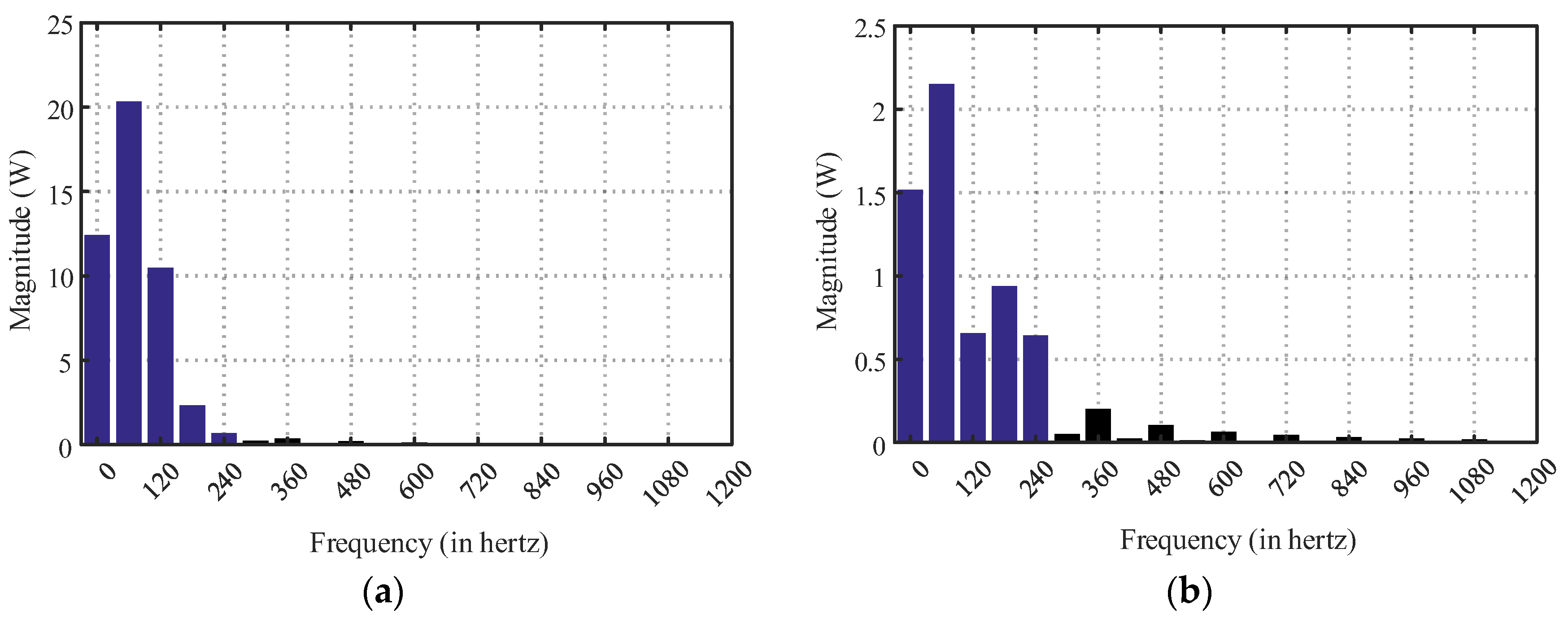
Figure 3 shows the FFTs of the sample IGBT and diode power loss waveforms.
As shown in 
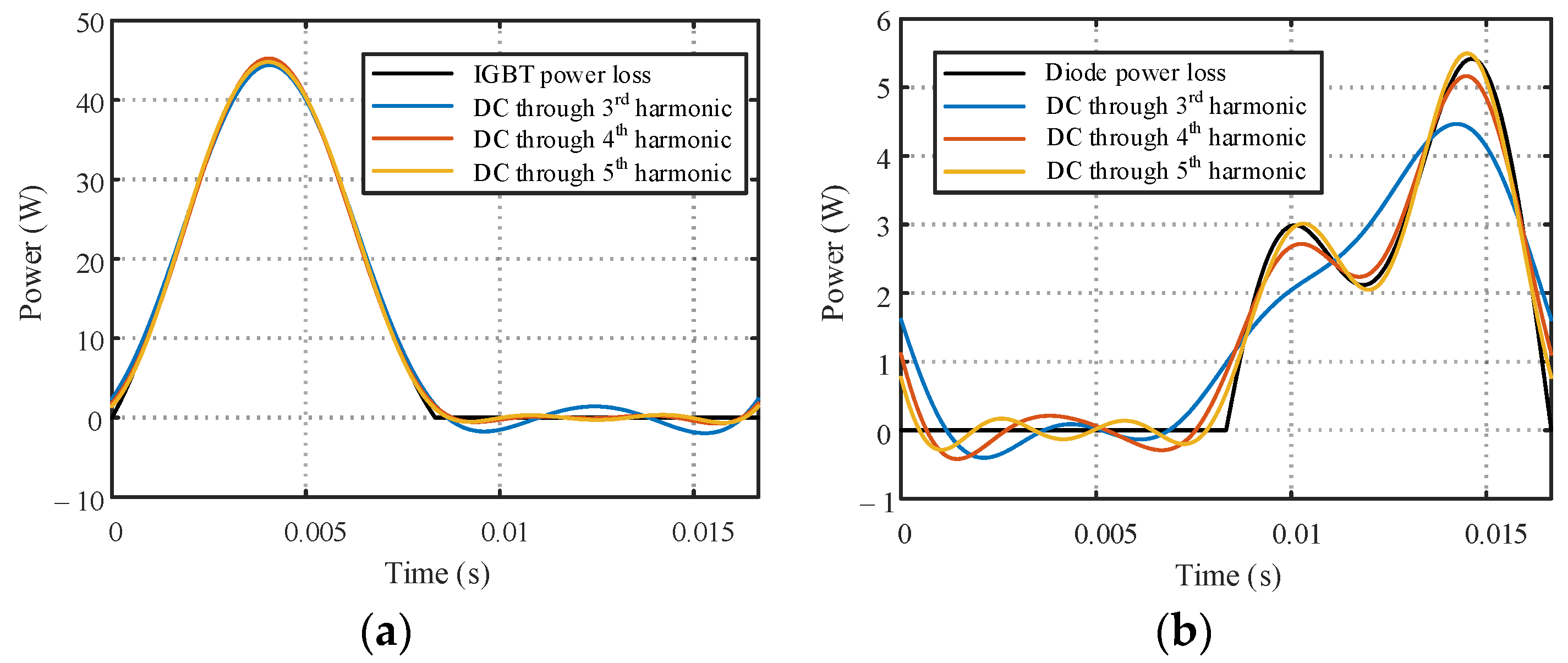
Figure 3, the magnitudes of the harmonics at frequencies greater than 240 Hz are relatively small and can therefore be neglected. The recovered power loss waveform from the inverse Fourier transform of the selected harmonics is shown in Figure 4, which contains the waveforms recovered from (1) dc to the third harmonic, (2) dc to the fourth harmonic, and (3) dc to the fifth harmonic. The recovered time-domain waveform with the dc to the fourth-order harmonics has already achieved an acceptable accuracy. Hence, in this study, we select the spectrum from dc to the fourth harmonics (240 Hz for a 60 Hz system) as the heat source for the junction temperature.
The selected harmonics from the power-loss FFT are then applied to the Foster model of the semiconductors to calculate the corresponding steady-state junction temperature in the frequency domain. The junction temperature phasors are then inversed back to the time domain to determine the junction temperature waveform. A sample of a recovered time-domain junction temperature is shown in Figure 5.

3. Fatigue Analysis

The fatigue analysis of PV inverter semiconductors involves two steps. The first step is to evaluate the junction temperature profile using a rainflow-counting algorithm. A rainflow-counting algorithm counts the number of thermal cycles and groups the thermal cycles by their average value and magnitude. The second step is to map the rainflow-counting results into semiconductor degradation. A semiconductor aging model is used to map each thermal cycle from the rainflow counting into semiconductor degradation.

3.1. Rainflow Counting

Rainflow counting is a standard algorithm used to evaluate the fatigue data of a system [45]. The basic idea of rainflow-counting algorithms is to count the strain cycle in a given period of time. Each strain cycle is described with three key parameters: the peak value, valley value, and the stress duration. For the rainflow-counting algorithm of inverter semiconductors, the strain is the junction temperature of each device. The peak and valley refer to the local maximum and minimum value of the junction temperature profile, respectively. The stress duration is the time period that starts with the valley of the cycle and ends with the peak of the cycle.
The rainflow counting algorithm is widely used in analysis of fatigue data in mechanical engineering to reduce a spectrum of varying stresses (strains) into a set of simple stress (strain) reversals. It enables the application of Miner’s rule in order to assess the accumulated fatigue of a structure subject to complex loading. The algorithm was developed by Tatsuo Endo and M. Matsuishi in 1968 to evaluate the fatigue of metals [46]. Downing and Socie created one of the most widely referenced and utilized rainflow cycle-counting algorithms in 1982, which was included as one of many cycle-counting algorithms in ASTM E 1049-85 (Standard Practices for Cycle Counting in Fatigue Analysis) [45]. Igor Rychlik proposed a mathematical definition for the rainflow-counting method, enabling closed-form computations based on the statistical properties of the load signal [47].
The rainflow-counting algorithm was named based on a comparison of the algorithm with the flow of rain falling on a pagoda and running down the edges of the roof. The rainflow-counting algorithm consists of the following steps:
  • Reduce the time history to a sequence of peaks and valleys;
  • Turn the sheet clockwise 90° (earliest time to the top);
  • Count the number of half cycles by looking for terminations in the flow occurring when either:
    • It reaches the end of the time history;
    • It merges with a flow that started at an earlier tensile peak; or
    • It flows when an opposite tensile peak has greater or equal magnitude.
  • Repeat step 3 for compressive valleys;
  • Assign a stress range (Δσ = σmax − σmin) to each half cycle equal to the stress difference between its start and termination;
  • Pair up half cycles starting from tensile peaks and compressive valleys with identical magnitude to count the number of complete cycles. Unmatched half cycles are residual half cycles.
A given half cycle may contain smaller half cycles. As a general rule, large stress cycles must not be fragmented into smaller cycles, which leads to underestimation of fatigue damage. Smaller stress cycles should be treated as temporary interruptions of larger stress reversals.
Figure 6a–c show the thermal profile preparation for rainflow counting. The junction temperature is calculated according to the PV generation based on the procedure established in Section 2.3. Then, the peaks and valleys are recorded according to the junction temperature profile. The transitions between the peaks and valleys are not of interest in the fatigue simulation and are therefore removed.
A thermal stress history of a semiconductor is shown in Figure 7a. The thermal stress history is reduced to peaks and valleys in Figure 7b. Turn the Figure 7b clockwise 90° as shown in Figure 7c. Half cycle (A) starts at tensile peak 1 and terminates opposite a thermal stress with equal magnitude, i.e., tensile peak 2; the stress range is ΔTj = T2T1. Similarly, half cycles (B)–(F) are calculated accordingly. The results of tensile-peak counting are summarized in Table 6.
Similar half cycles are calculated for compressive stresses. Figure 7d shows the half-cycles that start from compressive valleys. Half cycle (A) starts at compressive valley 1 and terminates opposite a thermal stress with equal magnitude, i.e., compressive valley 2; the stress range is ΔTj = T2T1. Similarly, half cycles (B)–(F) are calculated accordingly. The results of compressive-valley counting are summarized in Table 7.
The half cycles are then matched by the stress range and mean value. A pair of matched half cycles (one tension and one compression) is counted as a full cycle (or 1 cycle); an unmatched half cycle is counted as a half cycle (or 0.5 cycle). The results of half-cycle matching are summarized in Table 8.
The complete peak–valley profile can be fed into the rainflow-counting algorithm. However, considering the massive amount of data the complete peak–valley profile might contain, it is not be computationally efficient for a long-term simulation.

3.2. Reduced Thermal Profile

The complete peak–valley profile typically contains a massive amount of data. The semiconductor junction temperature typically cycles in a fundamental frequency (60 Hz or 50 Hz, depending on the region), as shown in Figure 6. Each fundamental period contains one peak and one valley. If all peaks and valleys are recorded, a 15 min peak–valley profile contains 108,000 data points, and a 3-year peak–valley profile contains more than one billion data points.
Studies have shown that low-frequency, large thermal cycling (which may occur only a few times each day) is the leading factor contributing to semiconductor aging [5,6,48]. High-frequency 60 Hz (or 50 Hz) thermal cycling contributes minimally to semiconductor aging [5,6,48] because 60 Hz (or 50-Hz) thermal cycling typically involves small strains (∆Tj), which fall into the elastic region of the stress–strain curve [6]. In the elastic region, it is assumed that no damage occurs during cycling [5]. Similar results were reported in [48].
The complete strain profile is typically reduced to a smaller set of profiles by discarding small stress cycles before applying the rainflow-counting algorithm [49]. Therefore, the 60/50 Hz thermal cycling in the semiconductor junction temperature profile can be neglected to accelerate the rainflow-counting algorithm.
In this study, only the first fundamental thermal cycling is kept for each PV sampling period. For example, if the PV sampling rate is one data point per 15 min, then only the first peak and valley are recorded in a 15 min simulation. The remaining peaks and valleys are disregarded. Peak–valley profile reduction can be explained with the aid of Figure 6d. The reduced thermal profile considerably reduces the number of data points if the sampling rate of PV generation is much slower than the fundamental period (60 Hz or 50 Hz). The detailed steps of rainflow counting using a reduced thermal profile are shown in Figure 8.
A sample thermal stress history of a semiconductor is shown in Figure 8a. The thermal stress history is reduced to peaks and valleys in Figure 8b. Fundamental frequency (50/60 Hz) thermal cycles are disregarded, except for the first peak and valley of each load change. Turn the Figure 8b clockwise 90° as shown in Figure 8c. Half cycle (A) starts at tensile peak 1 and terminates opposite a thermal stress with a larger magnitude, i.e., tensile peak 2; the stress range is ΔTj = T2T1. Similarly, half cycles (B) and (C) are calculated accordingly. The results of tensile-peak counting are summarized in Table 9.
Similar half cycles are calculated for compressive stresses. Figure 8d shows the half-cycles that start from compressive valleys. Half cycle (A) starts at compressive valley 1 and terminates opposite a thermal stress with an equal magnitude, i.e., compressive valley 2; the stress range is ΔTj = T2T1. Similarly, half cycles (B) and (C) are calculated accordingly. The results of compressive-valley counting are summarized in Table 10.
The half cycles are then matched by the stress range and mean value. The results of half-cycle matching are summarized in Table 11. A comparison of the results presented in Table 8 and Table 11 reveals the following: (1) the number of cycles of the stress range (T2T1) in Table 11 is less than that in Table 8; (2) Table 11 does not include the stress range (T4T3), whereas Table 8 includes one cycle in the stress range (T4T3); and (3) the number of cycles of the stress range (T4T1) is one in both Table 8 and Table 11. The reduced thermal profile only decreases the number of cycles for the small stress range, which cycles in the fundamental period (60 Hz in this example), and does not influence the number of cycles for the larger stress ranges.

3.3. Accumulated Fatigue Model

The rainflow-counting result can be mapped to semiconductor fatigue using the semiconductor aging model. The aging model of semiconductors is an empirical equation used to associate aging factors with lifetime expectation. For instance, the semiconductor aging model used in this study is based on [6,7,22,27],
N f = A × ( Δ T j ) α × ( a r ) β 1 Δ T j + β 0 × [ C + ( t o n ) γ C + 1 ] × exp ( E 1 k b × T ¯ j ) × f d
where Nf is the number of cycles to failure, indicating that a new semiconductor device will fail after Nf cycles of use under a given operating condition; T ¯ j is the mean junction temperature of a semiconductor; Δ T j is the junction temperature variation in a thermal cycle; and ton is the time from the valley to the peak. The other parameters are related to the semiconductor material physics and are given in Table 12 [27]. The aging model is tested in such a way that a periodic thermal stress is applied to a semiconductor until it fails. The thermal stress is applied from 0 to ton of each period, and the thermal stress is released from ton to the end of the period. The applied thermal stress has a variation of Δ T j and a mean temperature of T ¯ j . The semiconductor is expected to fail after Nf cycles under this test condition. The aging model presented in (1) is derived based on limited experimental conditions. The accuracy of such a model with larger ton has not yet been experimentally validated. However, the derivation and the accuracy of such a lifetime model is not the focus of this paper.
The rainflow-counting algorithm decomposes the thermal profile into several groups. Each group may contain thermal cycles that have identical thermal stress magnitudes ( Δ T j ), average junction temperatures ( T ¯ j ), and stress durations (ton). Each group can be mapped onto the number of semiconductor cycles to failure by calculating (1). The resulting Nf is the number of cycles to failure given the conditions Δ T j , T ¯ j , and ton. For example, if the rainflow-counting algorithm indicates that the mission profile contains n cycles of thermal stress under condition i, the number of cycles to failure (Nf) of this condition can be calculated using (1). In other words, the semiconductor is expected to fail after Nf cycles if continuously operated under this condition. Because the mission profile contains n cycles under such conditions, the accumulated life consumption under such conditions is n/Nf. Thus, the remaining life of the semiconductor is (100%—n/Nf). This accumulated damage calculation is also called Miner’s rule [50].
Various cumulative damage models have been proposed in the literature for reliability assessment [50,51,52]. The accumulated damage model used in this study follows Miner’s rule, which is a linear cumulative damage model [50]. The assumption of Miner’s rule is that the damage of the IGBT modules is independent of the stresses experienced during its life cycle, which means that each stress cycle from rainflow counting creates separate, independent damage. The sum of the damage from all rainflow cycles is the accumulated damage of the device. The accumulated fatigue can be expressed as follows,
A F = i n f , i N f , i
where Nf,i is the number of cycles to failure under condition i, and nf,i is the number of cycles to which the device is exposed under condition i. nf,i is obtained by the rainflow-counting algorithm.

4. Comparison Study

Most fatigue simulations need to reduce the junction temperature profile to accelerate the computational speed of the rainflow counting. The most common approach to reduce the thermal profile is to average the junction temperature every fundamental cycle (50 or 60 Hz). The basic idea of junction temperature averaging is to find the average junction temperature of the semiconductor over the fundamental cycle and disregard the small thermal cycling dynamics of the semiconductor. In this section, we discuss the differences between the common averaging approach and the FFT approach proposed in this paper.
The junction temperature-averaging approach is essentially a special case of the FFT approach proposed in this paper. Instead of restricting the dc to fourth harmonics, the averaging approach is equivalent to keeping just the dc component of the power loss. Figure 9 shows the junction temperature profile in a fundamental cycle using the FFT approach and the averaging approach.
The average approach can effectively disregard the small temperature cycles including the actual peak-and-valley values, which slightly modifies the rainflow-counting result. 
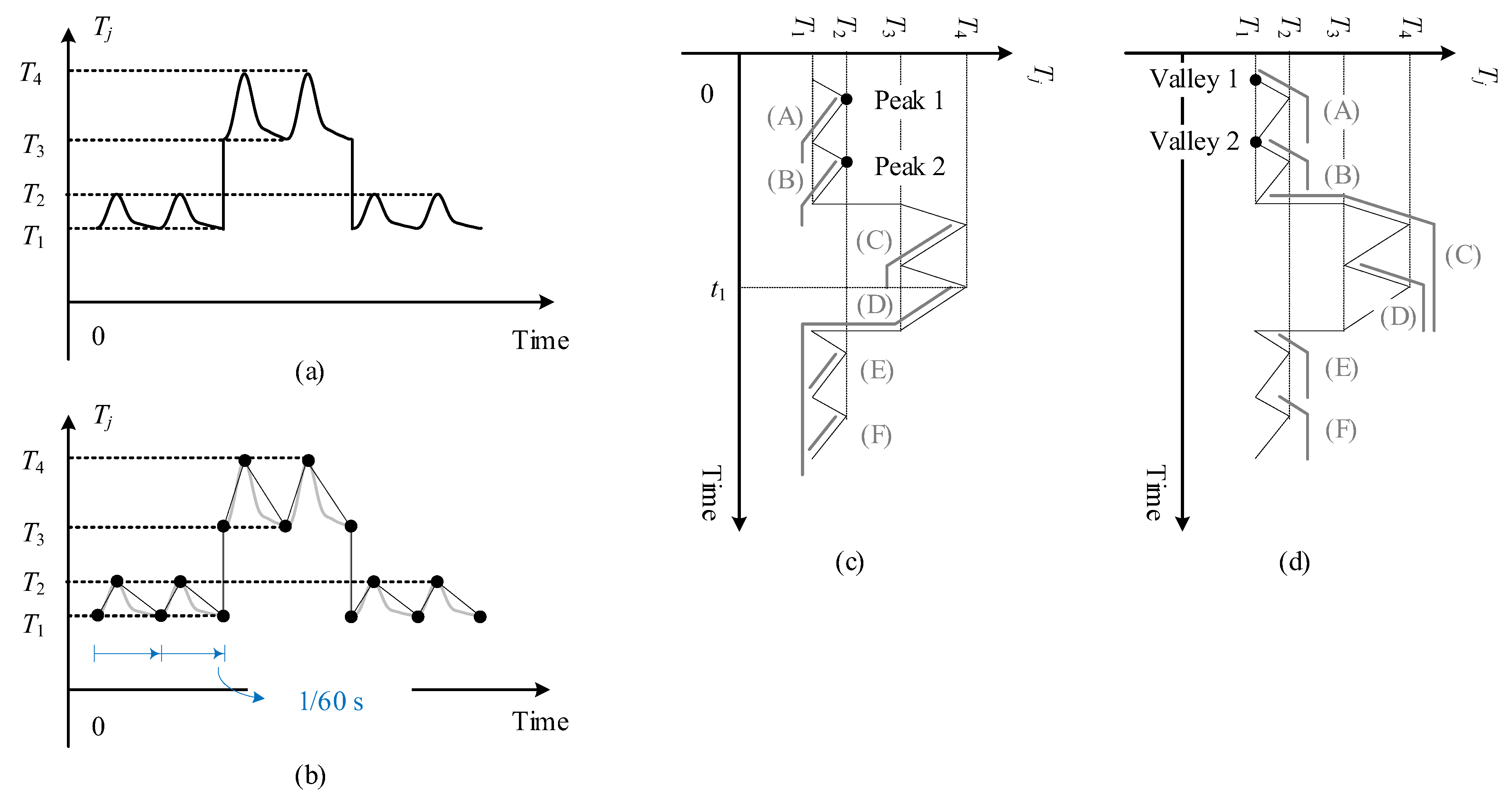
Figure 10 shows a sample rainflow counting applied to a semiconductor thermal profile using the average approach. The result of the rainflow counting shown in Figure 10 is that the profile contains one full cycle of thermal stress with a stress range of ∆Tj, where ∆Tj is less than T4T1. A comparison of the result of the average approach with that of the FFT approach shows that the average approach, in general, results in smaller thermal cycle magnitudes than the FFT approach. The average approach may not differ significantly from the FFT approach when the fundamental thermal cycling is small, for example, when the inverter is under a light loading condition. The averaging approach results in a more significant difference when the fundamental thermal cycling is large, for example, when the inverter is under a heavy loading condition.
To map the rainflow counting result onto the actual semiconductor aging, empirical semiconductor aging models are typically used [6,7,14]. Differences relative to available aging models will not be discussed in this paper. A comparison of the available fatigue simulations is summarized in Table 13. The proposed method (FFT + reduced thermal profile) can effectively keep the peak-and-valley profile for the semiconductors while accelerating the computational speed of rainflow counting.
In the following section, case studies are provided, and the proposed method is compared with the rainflow-counting algorithm using the complete peak–valley profile to demonstrate the effectiveness of the reduced thermal profile in accelerating the simulation speed.

5. Case Study

The proposed fatigue simulation was developed in MATLAB, a flow chart of which is shown in Figure 11. The PV generation profile is provided to the simulation, and the power loss of each semiconductor is then calculated accordingly. The power loss is fed into the FFT-based junction temperature calculation. Then, the semiconductor thermal profile is fed into the rainflow-counting algorithm to determine the device stress profile. The stress profile from rainflow counting is mapped to the accumulated fatigue result. A two-year PV inverter generation dataset is provided to the fatigue simulation. The data are from a sampled MPPT profile of a PV inverter in Chattanooga, Tennessee, from 1st August 2014 to July 2016. The time step of the dataset is 15 min. In the following case study, the first seven-day data from the two-year dataset are tested using (1) the complete thermal profile, (2) the reduced thermal profile, and (3) the averaged thermal profile. The complete two-year dataset is tested using the reduced and averaged thermal profiles only.

5.1. Junction Temperature Profile

Both the complete and reduced peak–valley plot of the semiconductor junction temperature are analyzed in this section. As discussed in Section 3.2, the complete peak–valley profile may contain 108,000 datapoints in a 15 min simulation, whereas the reduced peak–valley profile contains 4 datapoints. The complete and reduced peak–valley profiles from the simulation are shown in Figure 12. Four representative days are selected over the period from August 2014 to May 2015, among which 4 August 2014 is a sunny day, 11 May 2015 is partially cloudy, and 11 November 2014 and 15 February 2015 are cloudy. The zoomed-in figure for the complete peak–valley profile shows the 60 Hz cyclic junction temperature. The reduced peak–valley profile only keeps the first 60 Hz cyclic junction temperature and removes the rest. The overall picture for both complete and reduced peak–valley plots are similar, owing to the low resolution once the peak–valley plots are zoomed-out.

5.2. Rainflow Counting

The rainflow-counting algorithm is tested with (a) 7-day complete peak–valley profile, (b) 7-day reduced peak–valley profile, (c) 7-day averaged peak–valley profile, (d) 2-year reduced peak–valley profile, and (e) 2-year averaged peak–valley profile. The rainflow-counting results are displayed in Figure 13. Figure 13a–c show the 7-day rainflow counting results using the complete peak–valley profile, reduced peak–valley profile, and averaged peak–valley profile, respectively. The rainflow-counting results shown in Figure 13a,b are similar. Both results show that the thermal cycles can be categorized into three groups. Group 1 refers to the cycles with low frequency; these cycles are caused by solar irradiance variation, which typically varies from a few seconds to a few hours. The main causes of changes in solar irradiance are solar angle change, cloud cover, and temporary bird (or other object or animal) shading. Diurnal temperature variation also contributes to the low-frequency cycles in group 1. Group 2 refers to cycles with a 60 Hz frequency during the period in which the PV inverter generates active power (daylight). Group 3 refers to cycles with a 60 Hz frequency while the PV inverter is idling (night). Figure 13c does not show a 60 Hz cycle, as the averaged approach eliminates high-frequency cyclic temperatures in general.
The number of cycles for each group is summarized in Table 14. Group 1 refers to the peak–valleys with large Δ T j (greater than 5 °C). Group 2 refers to the peak–valleys with relatively small Δ T j (between 0.02 to 5 °C). Group 3 refers to the peak–valleys with extremely small Δ T j (less than 0.02 °C). The complete thermal profile contains a large number of thermal cycles from groups 2 and 3 (on the order of 107), whereas a relatively small number of thermal cycles from group 1 (125 cycles) is included. The reduced thermal profile and the averaged thermal profile have a similar number of thermal cycles from group 1 as the complete thermal profile. However, there a significantly fewer thermal cycles from groups 2 and 3 than from the complete thermal profile.

5.3. Accumulated Fatigue

The accumulated fatigue results from the 7-day simulation are summarized in Table 14. The accumulated fatigue of the IGBT is 0.4890% from the complete thermal profile, whereas the accumulated fatigue of the IGBT is 0.4882% from the reduced thermal profile and 0.3543% from the averaged thermal profile. The error of the reduced thermal profile is 0.16%, which is acceptable in fatigue simulation. However, the error of the averaged thermal profile is 27.55%, which may not be acceptable in fatigue simulations. The accumulated fatigue of the diode is 0.3228% for both the complete and reduced thermal profiles, whereas the accumulated fatigue of the diode is 0.2849% for the averaged thermal profile. The error of the averaged thermal profile is 11.74%, which may not be acceptable in fatigue simulations. Because the averaged thermal profile eliminates all original peaks and valleys, the simulated thermal cycle magnitude is reduced. As a result, the accumulative fatigue results tend to be underestimated.
The accumulated fatigue result shows that low-frequency thermal cycling is the leading factor contributing to the aging of the PV inverter semiconductor. In contrast, 60 Hz thermal cycling (groups 2 and 3) only contributes to a minor aging effect.
Table 15 and Table 16 show the two-year accumulated fatigue results from the reduced thermal profile and averaged thermal profile, respectively. For the reduced thermal profile, the 2-year simulation shows that the accumulated fatigues of the IGBT and diode are 20.85% and 13.98%, respectively, over the 2-year simulation (summarized in Table 15). This means that the remaining life of the IGBT and diode are 79.15% and 86.02%, respectively. The expected lifetime can be calculated as
t l i f e = 100 % 100 % A F t s i m
where AF is the accumulated fatigue (20.85% for IGBT and 13.98% for the diode), and tsim is the simulation time (two years). The IGBT and diode are expected to have a lifetime of 9.59 years and 14.31 years, respectively, given the simulated condition. Thus, the IGBTs determine the overall lifetime of the PV inverter instead of the diodes in this case.
For the averaged thermal profile shown in Table 16, the accumulated fatigue is 10% to 25% less than the result from the reduced profile. As stated in Section 4, the averaged method tends to underestimate the accumulated fatigue result because all 60 Hz cyclic data are eliminated.

5.4. Computation Time

The computation time of each stage of the fatigue simulation is recorded. The computation time is summarized in Table 17. Rainflow counting takes 20.21 s to process the 7-day data using the complete peak–valley profile, whereas it only takes 0.0012 s to process the same dataset using the reduced thermal profile. The total computation time of the 2-year simulation is 18.68 s using the reduced thermal profile. The junction temperature calculation accounts for most of the computation time in the 2-year simulation, whereas rainflow counting only takes 0.044 s. The averaged thermal profile requires the least computation time among all three profiles. The averaged thermal profile can save 1 s in junction temperature calculation and 0.3 s in rainflow-counting calculation compared to the proposed reduced thermal profile. The reduced thermal profile mainly focuses on reducing the peak–valley profile for rainflow counting, whereas the junction temperature calculation remains the same as the complete thermal profile. Therefore, the speed of junction temperature calculation with the reduced thermal profile is similar to that with the complete thermal profile. Accordingly, the junction temperature calculation accounts for most of the computation time for the 2-year simulation.

5.5. Transactive Energy System

In this case study, a PV inverter that serves a transactive energy system (TES) is simulated using the fatigue simulation proposed in this paper to demonstrate the potential use of the proposed simulation. A TES is a concept for distributed systems or microgrid operation to engage more distributed energy resources (DERs), especially non-utility-owned DERs connected to the power grid [53,54,55,56,57]. The basic idea of TES is to provide an incentive to customers to engage support from non-utility-owned DERs. A double-auction method is applied to determine the cleared price of a bidding. The PV inverter considered in this case study adopts the double-auction bidding strategy to determine the reactive power production [53]. PV inverters that adopt TES are requested to provide reactive power during extreme events. Therefore, the expected lifetime of such inverters is shorter compared to inverters that generate active power only. In this study, we use the proposed simulation to quantify the lifetime reduction caused by the TES. The active power generation of the PV inverter follows maximum power point tracking (MPPT).
Two electric rates (USD 0.101/kWh and USD 0.201/kWh) are tested in the simulation. PV owners are paid if any inverter power loss is introduced by reactive power generation. If the electric rate is high for real power, the utility may not be willing to purchase reactive power from customer-owned DERs because they need to monetarily compensate for any power loss generated by reactive power production [53,57]. Therefore, an increased electric rate leads to reduced reactive power generation from the PV inverter. Similarly, a reduced electric rate incentivizes increased reactive power generation. The power generation from the PV inverter during the 2-year simulation is summarized in Table 18. The active power production under the two electric rates is equivalent, whereas the reactive power production in the two TES cases differs by 2 Mvarh. The MPPT case presented in Table 18 refers to the test case discussed in Section 5.3 and Table 17. The 0.29 Mvarh reactive power from the MPPT case is the inverter’s inherent reactive power production.
Table 17 also summarizes the remaining lifetime for the inverter semiconductors. Compared with the MPPT case, the PV inverter semiconductors have less lifetime remaining for TES cases as a result of reactive power production. In the two TES cases with differing reactive power production, the TES case with less reactive power production (2.59 Mvarh) has more lifetime remaining in the 2-year simulation. The simulation also shows that IGBTs are more vulnerable than diodes in a PV inverter for all three test cases, as the remaining lifetime of IGBTs is less than that of diodes in general. The detailed monthly remaining-lifetime results are shown in Figure 14. The remaining-lifetime result could potentially guide the bidding strategy of the TES to help prevent overuse of the PV inverter.

6. Conclusions

In this paper, we propose a quasi-static time-series fatigue simulation for PV inverter semiconductors. The proposed fatigue simulation is suitable for degradation evaluation with long-term data and cosimulation with other quasi-static simulation platforms for power systems. The proposed simulation increases the time step from 100 μs (as used in conventional Euler–Maruyama-based simulation tools) to 15 min so that the simulation time step is consistent with the solar data time step. Small-junction temperature cycling is disregarded to accelerate the rainflow counting. The simulation results show that small thermal cycling contributes to an insignificant aging effect on the semiconductors. The reduced thermal profile can correctly predict the accumulated fatigue. The error of the reduced thermal profile is 0.16%, which is acceptable in fatigue simulation. Compared to the conventional averaged thermal profile, the proposed reduced thermal profile can successfully maintain the actual peak and valley information with only a moderate computation time. As a result, the reduced thermal profile is significantly more accurate than the averaged thermal profile. A TES test case is presented to demonstrate the use of the proposed fatigue simulation. The proposed simulation can potentially be used to develop new system control strategies and evaluate inverter semiconductor degradation for a given grid code.

Author Contributions

Conceptualization, Y.L. and L.M.T.; methodology, Y.L., L.M.T. and P.K; software, Y.L.; validation, Y.L.; formal analysis, Y.L.; investigation, Y.L., L.M.T., P.K., J.D., L.Z., K.P.S. and K.P.; resources, L.M.T., P.K. and K.P.S.; data curation, Y.L. and L.M.T.; writing—original draft preparation, Y.L.; writing—review and editing, Y.L., L.M.T., P.K., J.D., L.Z., T.B.O., K.P.S. and K.P.; visualization, Y.L.; supervision, L.M.T. and K.P.S.; project administration, L.M.T. and K.P.S.; funding acquisition, L.M.T. and K.P.S. All authors have read and agreed to the published version of the manuscript.

Funding

This work was primarily supported by the U.S. Department of Energy Grid Modernization Laboratory Consortium. This work also made use of Engineering Research Center shared facilities supported by the Engineering Research Center Program of the National Science Foundation and the Department of Energy under NSF Award Number (EEC-1041877) and the CURENT Industry Partnership Program.

Data Availability Statement

Not applicable.

Conflicts of Interest

The authors declare no conflict of interest.

References

  1. Woodhouse, M.; Jones-Albertus, R.; Feldman, D.; Fu, R.; Horowitz, K.; Chung, D.; Dirk, J.; Sarah, K. On the Path to SunShot: The Role of Advancements in Solar Photovoltaic Efficiency, Reliability, and Costs; NREL/TP-6A20-65872; National Renewable Energy Lab: Golden, CO, USA, 2016. [Google Scholar]
  2. Golnas, A. PV system reliability: An operator’s perspective. IEEE J. Photovolt. 2013, 1, 416–421. [Google Scholar] [CrossRef]
  3. Yang, S.; Bryant, A.; Mawby, P.; Xiang, D.; Ran, L.; Tavner, P. An industry-based survey of reliability in power electronic converters. IEEE Trans. Ind. Appl. 2011, 47, 1441–1451. [Google Scholar] [CrossRef]
  4. Yuan, Q.; Endoh, R.; Ima, T.; Kajita, Y.; Luo, Y. Failure Mode Verification of Power IGBT under Different Thermal Stress Application Conditions in Power Cycling Test Environment. In Proceedings of the 2018 International Conference on Electronics Packaging and iMAPS All Asia Conference (ICEP-IAAC), Mie, Japan, 17–21 April 2018; pp. 367–370. [Google Scholar] [CrossRef]
  5. McPherson, J.W.; Ogawa, E.T. Reliability Physics and Engineering Time-to-Failure Modeling, 2nd ed; Springer: Berlin/Heidelberg, Germany, 2007. [Google Scholar]
  6. Wang, H.; Ma, K.; Blaabjerg, F. Design for Reliability of Power Electronic Systems. In Proceedings of the IECON 2012-38th Annual Conference on IEEE Industrial Electronics Society, Montreal, QC, Canada, 25–28 October 2012; pp. 33–44. [Google Scholar] [CrossRef]
  7. Scheuermann, U.; Schmidt, R.; Newman, P. Power Cycling Testing with Different Load Pulse Durations. In Proceedings of the 7th IET International Conference on Power Electronics, Machines and Drives, Manchester, UK, 8–10 April 2014; pp. 1–6. [Google Scholar] [CrossRef]
  8. Andresen, M.; Buticchi, G.; Liserre, M. Thermal Stress Analysis and MPPT Optimization of Photovoltaic Systems. IEEE Trans. Ind. Electron. 2016, 63, 4889–4898. [Google Scholar] [CrossRef] [Green Version]
  9. Yang, Y.; Wang, H.; Blaabjerg, F. Improved Reliability of Single-Phase PV Inverters by Limiting the Maximum Feed-in Power. In Proceedings of the 2014 IEEE Energy Conversion Congress and Exposition (ECCE), Pittsburgh, PA, USA, 14–18 September 2014; pp. 128–135. [Google Scholar] [CrossRef] [Green Version]
  10. Sangwongwanich, A.; Yang, Y.; Sera, D.; Blaabjerg, F. Impacts of PV Array Sizing on PV Inverter Lifetime and Reliability. In Proceedings of the 2017 IEEE Energy Conversion Congress and Exposition (ECCE), Cincinnati, OH, USA, 1–5 October 2017; pp. 3830–3837. [Google Scholar] [CrossRef] [Green Version]
  11. He, J.; Sangwongwanich, A.; Yang, Y.; Iannuzzo, F. Lifetime Evaluation of Three-Level Inverters for 1500-V Photovoltaic Systems. IEEE J. Emerg. Sel. Top. Power Electron. 2020, 9, 4285–4298. [Google Scholar] [CrossRef]
  12. Ravyts, S.; Van De Sande, W.; Daenen, M.; Driesen, J.; Cappelle, J. Impact of Conduction Mode and Phase-Shedding Strategy on Transistor Lifetime in Building-Integrated Photovoltaics Module-Level Converters. In Proceedings of the 2021 23rd European Conference on Power Electronics and Applications, Ghent, Belgium, 6–10 September 2021; pp. P.1–P.10. [Google Scholar] [CrossRef]
  13. Acuna, J.; Rupp, T.; Sonner, M.; Klingler, M.; Metais, B.; Kallfass, I. Influence of Power Cycle On-State Duration on the Lifetime of Power Module Die-Attach Layers. In Proceedings of the 2019 25th International Workshop on Thermal Investigations of ICs and Systems (THERMINIC), Lecco, Italy, 25–27 September 2019; pp. 1–6. [Google Scholar] [CrossRef]
  14. Bayerer, R.; Herrmann, T.; Licht, T.; Lutz, J.; Feller, M. Model for Power Cycling lifetime of IGBT Modules—Various Factors Influencing Lifetime. In Proceedings of the 5th International Conference on Integrated Power Electronics Systems, Nuremberg, Germany, 11–13 March 2008; pp. 1–6. [Google Scholar]
  15. Ceccarelli, L.; Kotecha, R.M.; Bahman, A.S.; Iannuzzo, F.; Mantooth, H.A. Mission-Profile-Based Lifetime Prediction for a SiC mosfet Power Module Using a Multi-Step Condition-Mapping Simulation Strategy. IEEE Trans. Power Electron. 2019, 34, 9698–9708. [Google Scholar] [CrossRef]
  16. Ristow, A.; Begovic, M.; Pregelj, A.; Rohatgi, A. Development of a Methodology for Improving Photovoltaic Inverter Reliability. IEEE Trans. Ind. Electron. 2008, 55, 2581–2592. [Google Scholar] [CrossRef]
  17. Aziz, T.; Ketjoy, N. PV Penetration Limits in Low Voltage Networks and Voltage Variations. IEEE Access 2017, 5, 16784–16792. [Google Scholar] [CrossRef]
  18. Yang, Y.; Wang, H.; Blaabjerg, F. Reliability Assessment of Transformerless PV Inverters considering Mission Profiles. Int. J. Photoenergy 2015, 2015, 968269. [Google Scholar] [CrossRef]
  19. Wei, W.; Xu, G.; Qiu, X. A Novel Assessment Method of Gate Oxide Degradation Based on IGBT Turn-on Losses for on-Line Reliability Monitoring. In Proceedings of the 2019 International Conference on Intelligent Computing, Automation and Systems (ICICAS), Chongqing, China, 6–8 December 2019; pp. 243–248. [Google Scholar] [CrossRef]
  20. Wang, Z.; Tian, B.; Qiao, W.; Qu, L. Real-Time Aging Monitoring for IGBT Modules Using Case Temperature. IEEE Trans. Ind. Electron. 2015, 63, 1168–1178. [Google Scholar] [CrossRef]
  21. Givaki, K.; Jamieson, P.; Parker, M. Estimation of the Power Electronic Converter Lifetime in Fully Rated Converter Wind Turbine for Onshore and Offshore Wind Farms. In Proceedings of the 7th IET International Conference on Power Electronics, Machines and Drives, Manchester, UK, 8–10 April 2014; pp. 1–6. [Google Scholar] [CrossRef] [Green Version]
  22. Sangwongwanich, A.; Wang, H.; Blaabjerg, F. Reduced-Order Thermal Modeling for Photovoltaic Inverters Considering Mission Profile Dynamics. IEEE Open J. Power Electron. 2020, 1, 407–419. [Google Scholar] [CrossRef]
  23. Bryant, A.T.; Mawby, P.A.; Palmer, P.R.; Santi, E.; Hudgins, J.L. Exploration of Power Device Reliability Using Compact Device Models and Fast Electrothermal Simulation. IEEE Trans. Ind. Appl. 2008, 44, 894–903. [Google Scholar] [CrossRef]
  24. Ma, X.; Guo, Y.; Wang, L.; Ji, W. Exploration of the Reliability of Automotive Electronic Power Steering System Using Device Junction Electrothermal Profile Cycle. IEEE Access 2016, 4, 7054–7062. [Google Scholar] [CrossRef]
  25. Lv, G.; Lei, W.; Wang, M.; Lv, C.; Zhao, J. Reliability Analysis and Design of MMC Based on Mission Profile for the Components Degradation. IEEE Access 2020, 8, 149940–149951. [Google Scholar] [CrossRef]
  26. Shen, Z.; Dinavahi, V. Real-Time Device-Level Transient Electrothermal Model for Modular Multilevel Converter on FPGA. IEEE Trans. Power Electron. 2015, 31, 6155–6168. [Google Scholar] [CrossRef]
  27. Sangwongwanich, A.; Yang, Y.; Sera, D.; Blaabjerg, F. Lifetime Evaluation of Grid-Connected PV Inverters Considering Panel Degradation Rates and Installation Sites. IEEE Trans. Power Electron. 2017, 33, 1225–1236. [Google Scholar] [CrossRef] [Green Version]
  28. Sintamarean, N.C.; Wang, H.; Blaabjerg, F.; Rimmen, P.D.P. A design tool to study the impact of mission-profile on the reliability of SiC-based PV-inverter devices. Microelectron. Reliab. 2014, 54, 1655–1660. [Google Scholar] [CrossRef]
  29. Reigosa, P.D.; Wang, H.; Yang, Y.; Blaabjerg, F. Prediction of bond wire fatigue of IGBTs in a PV inverter under a long-term operation. IEEE Trans. Power Electron. 2015, 31, 7171–7182. [Google Scholar]
  30. Felgemacher, C.; Araujo, S.; Noeding, C.; Zacharias, P.; Ehrlich, A.; Schidleja, M. Evaluation of Cycling Stress Imposed on IGBT Modules in PV Central Inverters in Sunbelt Regions. In Proceedings of the CIPS 2016-9th International Conference on Integrated Power Electronics Systems, Nuremberg, Germany, 8–10 March 2016; pp. 1–6. [Google Scholar]
  31. De León-Aldaco, S.E.; Calleja, H.; Chan, F.; Jiménez-Grajales, H.R. Effect of the mission profile on the reliability of a power converter aimed at photovoltaic applications—A case study. IEEE Trans. Power Electron. 2012, 28, 2998–3007. [Google Scholar] [CrossRef]
  32. Chan, F.; Calleja, H. Reliability Estimation of Three Single-Phase Topologies in Grid-Connected PV Systems. IEEE Trans. Ind. Electron. 2010, 58, 2683–2689. [Google Scholar] [CrossRef]
  33. Koutroulis, E.; Blaabjerg, F. Design optimization of transformerless grid-connected PV inverters including reliability. IEEE Trans. Power Electron. 2013, 28, 325–335. [Google Scholar] [CrossRef] [Green Version]
  34. Flicker, J.; Johnson, J.; Hacke, P.; Thiagarajan, R. Automating Component-Level Stress Measurements for Inverter Reliability Estimation. Energies 2022, 15, 4828. [Google Scholar] [CrossRef]
  35. Kshatri, S.S.; Dhillon, J.; Mishra, S.; Tariq, R.; Sharma, N.K.; Bajaj, M.; Rehman, A.U.; Shafiq, M.; Choi, J.-G. Reliability Analysis of Bifacial PV Panel-Based Inverters Considering the Effect of Geographical Location. Energies 2021, 15, 170. [Google Scholar] [CrossRef]
  36. Choi, U.-M.; Lee, J.-S. Comparative Evaluation of Lifetime of Three-Level Inverters in Grid-Connected Photovoltaic Systems. Energies 2020, 13, 1227. [Google Scholar] [CrossRef] [Green Version]
  37. Mather, B.A. Quasi-Static Time-Series Test Feeder for PV Integration Analysis on Distribution Systems. In Proceedings of the 2012 IEEE Power and Energy Society General Meeting, San Diego, CA, USA, 22–26 July 2012; pp. 1–8. [Google Scholar] [CrossRef]
  38. Dugan, R.; Short, T.; Forsten, K. Modeling Energy Efficiency Alternatives for Distribution System Power Delivery. In Proceedings of the CIRED 2009-20th International Conference and Exhibition on Electricity Distribution-Part 1, Prague, Czech Republic, 8–11 June 2009. [Google Scholar] [CrossRef] [Green Version]
  39. Schneider, K.P.; Fuller, J.C. Voltage Control Devices on the IEEE 8500 Node Test Feeder. In Proceedings of the IEEE PES Transmission and Distribution Conference and Exposition, New Orleans, LA, USA, 19–22 April 2010; pp. 1–6. [Google Scholar] [CrossRef]
  40. Liu, Y.; Tolbert, L.M.; Kritprajun, P.; Dong, Q.; Zhu, L.; Hambrick, J.C.; Schneider, K.; Prabakar, K. Quasi-Static Time Series Fatigue Simulation for PV Inverter Semiconductors with Long-Term Solar Profile. In Proceedings of the 2021 IEEE Power & Energy Society General Meeting (PESGM), Washington, DC, USA, 26–29 July 2021; pp. 01–05. [Google Scholar] [CrossRef]
  41. Liu, Y.; Tolbert, L.M.; Kritprajun, P.; Dong, J.; Zhu, L.; Hambrick, J.; Schneider, K.P.; Prabakar, K. Aging Effect Analysis of PV Inverter Semiconductors for Ancillary Services Support. IEEE Open J. Ind. Appl. 2020, 1, 157–170. [Google Scholar] [CrossRef]
  42. Blake, C.; Bull, C. IGBT or MOSFET: Choose Wisely. International Rectifier. El Segundo, CA, USA. Available online: http://w5jgv.com/hv-ps1/pdf/choosewisely.pdf (accessed on 24 November 2022).
  43. Anurag, A.; Yang, Y.; Blaabjerg, F. Thermal Performance and Reliability Analysis of Single-Phase PV Inverters With Reactive Power Injection Outside Feed-In Operating Hours. IEEE J. Emerg. Sel. Top. Power Electron. 2015, 3, 870–880. [Google Scholar] [CrossRef]
  44. Wang, Z. Real-Time Internal Temperature Estimation and Health Monitoring for IGBT Modules. Ph.D. Thesis, The University of Nebraska-Lincoln, Lincoln, NE, USA, 2017. [Google Scholar]
  45. ASTM E1049; Standard Practices for Cycle Counting in Fatigue Analysis. ASTM Standards: West Conshohocken, PA, USA, 2017.
  46. Matsuishi, M.; Endo, T. Fatigue of metals subjected to varying stress. Jpn. Soc. Mech. Eng. 1968, 68, 37–40. [Google Scholar]
  47. Rychlik, I. A new definition of the rainflow cycle counting method. Int. J. Fatigue 1987, 9, 119–121. [Google Scholar] [CrossRef]
  48. Lai, W.; Chen, M.; Ran, L.; Alatise, O.; Xu, S.; Mawby, P. Low ΔTj stress cycle effect in IGBT power module die-attach lifetime modeling. IEEE Trans. Power Electron. 2015, 31, 6575–6585. [Google Scholar] [CrossRef]
  49. Schluter, L.L.; Sutherland, H.J. User’s Guide for LIFE2′s Rainflow Counting Algorithm; SAND90-2259; Sandia National Laboratories: Albuquerque, NW, USA; Livermore, CA, USA, 1991.
  50. Miner, M.A. Cumulative Damage in Fatigue. J. Appl. Mech. 1945, 12, A159–A164. [Google Scholar] [CrossRef]
  51. Ashby, M.F.; Jones, D.R.H. Engineering Materials 1—An Introduction to Properties, Applications and Design, 3rd ed.; Butterworth-Heinemann: Oxford, UK, 2005; p. 228. [Google Scholar]
  52. Huang, H.; Mawby, P.A. A Lifetime Estimation Technique for Voltage Source Inverters. IEEE Trans. Power Electron. 2012, 28, 4113–4119. [Google Scholar] [CrossRef]
  53. Alam, J.E.; Somani, A.; Melton, R.; McDermott, T. Transactive Approach for Engaging Distribution Network Assets for Voltage Management in Southern California Edison Distribution Feeders; Pacific Northwest National Lab. (PNNL): Richland, WA, USA, 2018. [Google Scholar] [CrossRef]
  54. Bhattarai, B.P.; Alam, J.; Hansen, J.; Schneider, K.; Radhakrishnan, N.; Somani, A.; Du, W. Enhancing Distribution System Resiliency through a Novel Transactive Energy Systems Framework. In Proceedings of the 2019 IEEE Power & Energy Society General Meeting (PESGM), Atlanta, GA, USA, 4–8 August 2019; pp. 1–5. [Google Scholar] [CrossRef]
  55. Li, J.; Zhang, C.; Xu, Z.; Wang, J.; Zhao, J.; Zhang, Y.-J.A. Distributed transactive energy trading framework in distribution networks. IEEE Trans. Power Syst. 2018, 33, 7215–7227. [Google Scholar] [CrossRef]
  56. Liu, Z.; Wu, Q.; Huang, S.; Zhao, H. Transactive Energy: A Review of State of the Art and Implementation. In Proceedings of the 2017 IEEE Manchester PowerTech, Manchester, UK, 18–22 June 2017; pp. 1–6. [Google Scholar]
  57. Liu, Y.; Kritprajun, P.; Tolbert, L.M.; Dong, J.; Zhu, L.; Hambrick, J.C.; Schneider, K.; Bhattarai, B.P. Modeling of Marginal Cost for PV Inverter Ancillary Services Considering Inverter Aging under Transactive Energy Framework. In Proceedings of the 2020 IEEE Power & Energy Society General Meeting (PESGM), Montreal, QC, Canada, 2–6 August 2020; pp. 1–5. [Google Scholar] [CrossRef]
Figure 1. Typical two-stage, single-phase PV converter topology [41].
Energies 15 09104 g001
Figure 2. Detailed thermal model of a PV inverter using a discrete IGBT diode pack [40].
Energies 15 09104 g002
Figure 3. PV inverter (a) typical IGBT power-loss FFT and (b) typical diode power-loss FFT.
Energies 15 09104 g003
Figure 4. Inverse Fourier transform of (a) IGBT power loss and (b) diode power loss in a PV inverter.
Energies 15 09104 g004
Figure 5. Recovered time-domain diode and IGBT junction temperature for one electric cycle (60 Hz) in a PV inverter [40].
Energies 15 09104 g005
Figure 6. Thermal profile preparation for rainflow counting. (a) PV solar incidence data; (b) IGBT/diode junction temperature; (c) complete peak–valley profile; and (d) reduced peak–valley profile.
Energies 15 09104 g006
Figure 7. Example of rainflow counting for the semiconductor thermal profile. (a) Thermal stress history of a semiconductor. (b) Peak–valley history of a semiconductor. (c) Half cycles that start from tensile peaks. (d) Half cycles that start from compressive valleys.
Energies 15 09104 g007
Figure 8. Example of rainflow counting for a reduced thermal profile. (a) Thermal stress history of a semiconductor. (b) Peak–valley history of a semiconductor using a reduced thermal profile. (c) Half cycles that start from tensile peaks. (d) Half cycles that start from compressive valleys.
Energies 15 09104 g008
Figure 9. Comparison of the diode and IGBT junction temperatures for one electric cycle (60 Hz) using the FFT approach and the average approach.
Energies 15 09104 g009
Figure 10. Example of rainflow counting for the semiconductor thermal profile using the average approach. (a) Thermal stress history of a semiconductor. (b) Peak–valley history of a semiconductor.
Energies 15 09104 g010
Figure 11. Flow chart of the proposed fatigue simulation [40].
Energies 15 09104 g011
Figure 12. IGBT and diode junction temperature profile for a PV inverter with 7 days of insolation data. (a) Sample complete peak–valley profile for 4 August 2014; (b) sample reduced peak–valley profile for 4 August 2014; (c) sample complete peak–valley profile for 11 November 2014; (d) sample reduced peak–valley profile for 11 November 2014; (e) sample complete peak–valley profile for 15 February 2015; (f) sample reduced peak–valley profile for 15 February 2015; (g) sample complete peak–valley profile for 11 May 2015; and (h) sample reduced peak–valley profile for 11 May 2015.
Energies 15 09104 g012aEnergies 15 09104 g012b
Figure 13. Rainflow-counting results of the diode junction temperature profile for (a) 7-day complete peak–valley profile, (b) 7-day reduced peak–valley profile, and (c) 7-day averaged peak–valley profile.
Energies 15 09104 g013
Figure 14. Monthly remaining-lifetime remaining from the fatigue simulation. (a) MPPT; (b) TES with USD 0.101/kWh rate; and (c) TES with USD 0.201/kWh rate.
Energies 15 09104 g014aEnergies 15 09104 g014b
Table 1. Semiconductor power loss.
IGBTSwitching Loss ( E o n , I + E o f f , I ) f s w
Conduction Loss I r m s , I G B T 2 R I G B T + I a v g , I G B T V 0 , I G B T
MOSFETSwitching Loss ( E o n , M + E o f f , M ) f s w
Conduction Loss I r m s , M 2 R d s ( o n )
DiodeSwitching Loss ( 2 π I s V d c I r e f V r e f E r r , D ) f s w
Conduction Loss I r m s , D 2 R D + I a v g , D V 0 , D
Table 2. IGBT key parameters.
Part No.IKW60N60H3
ManufacturerInfineon
V0,IGBT1.06 V
RIGBT0.024 Ω
Tj175 °C
VGE0/15 V
VCE400 V
IC60 A
Eon2.63 mJ
Eoff1.46 mJ
Table 3. Diode key parameters.
Part No.IKW60N60H3
ManufacturerInfineon
V0,D0.76 V
RD0.025 Ω
Tj175 °C
Qrr2.8 μC
Vref400 V
Iref60 A
Table 4. Diode and IGBT (IKW60N60H3) Foster model.
Thermal Resistance (K/W)
R1R2R3R4R5
Diode0.0490.230.310.270.2
IGBT0.00340.0720.0820.1960.0093
Thermal Capacitance (s)
τ1τ2τ3τ4τ5
Diode7.50 × 10−62.20 × 10−42.3 × 10−31.55 × 10−20.108
IGBT3 × 10−52.7 × 10−43 × 10−31.56 × 10−20.2275
Table 5. Heat sink thermal parameters.
Heat sink part numberC247-025
ManufacturerOhmite
Surface area7312 mm2
Thermal resistance3~9 °C/W (5 °C/W for this paper)
Thermal capacitance1000 s
Table 6. Half-cycle counting for tensile peaks.
Tensile Half CycleStress Range ΔTj (°C) Mean   T ¯ j (°C)
(A)T2T1(T1 + T2)/2
(B)T2T1(T1 + T2)/2
(C)T4T3(T3 + T4)/2
(D)T4T1(T1 + T4)/2
(E)T2T1(T1 + T2)/2
(F)T2T1(T1 + T2)/2
Table 7. Half-cycle counting for compressive valleys.
Compressive Half CycleStress Range ΔTj (°C) Mean   T ¯ j (°C)
(A)T2T1(T1 + T2)/2
(B)T2T1(T1 + T2)/2
(C)T4T1(T1 + T4)/2
(D)T4T3(T3 + T4)/2
(E)T2T1(T1 + T2)/2
(F)T2T1(T1 + T2)/2
Table 8. Half-cycle matching and rainflow-counting results.
Stress Range ΔTj (°C)Full CyclesHalf Cycles
T2T140
T4T310
T4T110
Table 9. Half-cycle counting for tensile peaks in a reduced thermal profile.
Tensile Half CycleStress Range ΔTj (°C) Mean   T ¯ j (°C)
(A)T2T1(T1 + T2)/2
(B)T4T1(T1 + T4)/2
(C)T2T1(T1 + T2)/2
Table 10. Half-cycle counting for compressive valleys in a reduced thermal profile.
Compressive Half CycleStress Range ΔTj (°C) Mean   T ¯ j (°C)
(A)T2T1(T1 + T2)/2
(B)T4T1(T1 + T4)/2
(C)T2T1(T1 + T2)/2
Table 11. Half-cycle matching and rainflow-counting results using the reduced thermal profile.
Stress Range ΔTj (°C)Full CyclesHalf Cycles
T2T120
T4T110
Table 12. Parameters of the lifetime model of an IGBT module.
ParameterValueExperimental Condition
A3.4368 × 10145 °C ≤ ∆Tj ≤ 80 °C
α−4.923
β19.012 × 10⁻³
β01.9420.19 ≤ ar ≤ 0.42
C1.434
γ−1.2080.07 s ≤ ton ≤ 63 s
fd0.6204
Ea0.06606 eV 32.5   ° C     T ¯ j ≤ 122 °C
kB8.6173324 × 10−5 eV/K
Table 13. Comparison of the proposed aging simulation and aging simulations available in the literature.
Creating Mission ProfileRainflow CountingSemiconductor Aging Model
Proposed methodFull-order lumped thermal network + FFTReduced thermal profileAging model in [7] and Miner’s rule
Method in [6,27]Look-up table, full-order lumped thermal network + Euler methodAverage thermal profileAging model in [6,7] or [14] and Miner’s rule
Method in [28,29,30]Full-order lumped thermal network + Euler methodAverage thermal profileAging model in [14] and Miner’s rule
Method in [22]Reduced-order lumped thermal network + Euler methodAverage thermal profileAging model in [14] and Miner’s rule
Method in [31,32,33,34,35,36]Steady-state lumped thermal network + Euler methodAverage thermal profileAging model in [14] and Miner’s rule
Table 14. Accumulated fatigue results from the 7-day simulation.
Complete Thermal Profile
IGBTDiode
Fatigue Typeton (s)Number of CyclesAccumulated FatigueNumber of CyclesAccumulated Fatigue
Low-frequency cycling>1/1201250.4882%1250.3228%
60 Hz cycling1/1202.0304 × 1077.9904 × 10−4%2.0304 × 1079.0085 × 10−6%
Inverter idling1/1201.5984 × 1072.8396 × 10−18%1.5984 × 1076.4579 × 10−19%
Accumulated Fatigue0.4890%Accumulated Fatigue0.3228%
Reduced Thermal Profile
IGBTDiode
Fatigue Typeton (s)Number of CyclesAccumulated FatigueNumber of CyclesAccumulated Fatigue
Low-frequency cycling>1/1201270.4882%1270.3228%
60 Hz cycling1/1203231.0103 × 10−8%3231.1447 × 10−10%
Inverter idling1/1202224.6369 × 10−23%2229.5791 × 10−24%
Accumulated Fatigue0.4882%Accumulated Fatigue0.3228%
Averaged Thermal Profile
IGBTDiode
Fatigue Typeton (s)Number of CyclesAccumulated FatigueNumber of CyclesAccumulated Fatigue
Low-frequency cycling>1/1201250.3543%1250.2849%
60 Hz cycling1/12000%00%
Inverter idling1/12000%00%
Accumulated Fatigue0.3543%Accumulated Fatigue0.2849%
Table 15. Accumulated fatigue results from the two-year simulation with reduced thermal profile.
IGBTDiode
Fatigue TypeNumber of CyclesAccumulated FatigueNumber of CyclesAccumulated Fatigue
Low-frequency cycling12,89820.8543%12,88713.9768%
60 Hz cycling28,5244.5591 × 10−7% 5.0886 × 10⁻⁹%
Inverter idling28,6504.8181 × 10−21%28,5082.6372 × 10−21%
Accumulated Fatigue20.8543%Accumulated Fatigue13.9768%
Table 16. Accumulated fatigue results from the two-year simulation with averaged thermal profile.
IGBTDiode
Fatigue TypeNumber of CyclesAccumulated FatigueNumber of CyclesAccumulated Fatigue
Low-frequency cycling12,38115.3078%12,37312.3812%
60 Hz cycling00%00%
Inverter idling00%00%
Accumulated Fatigue15.3078%Accumulated Fatigue12.3812%
Table 17. Computation time comparison.
Junction Temperature CalculationRainflow Counting
Complete thermal profile7-day data2.34 s20.21 s
Reduced thermal profile7-day data0.18 s0.0012 s
2-year data18.64 s0.044 s
Averaged thermal profile7-day data0.20 s0.00072 s
2-year data17.71 s0.015 s
Table 18. Simulation result from the TES test cases.
MPPTTES
Electric Rate, USD 0.101/kWhElectric Rate, USD 0.201/kWh
P, MWh7.287.167.16
Q, Mvarh0.294.502.59
Remaining LifetimeDiode86.02%76.31%80.46%
IGBT79.15%68.17%72.93%
Publisher’s Note: MDPI stays neutral with regard to jurisdictional claims in published maps and institutional affiliations.

