

OrcaFlex Modelling of a Multi-Body Floating Solar Island Subjected to Waves

INNOSEA, Bâtiment Insula, 11 Rue Arthur III, 44200 Nantes, France
*
Author to whom correspondence should be addressed.
Energies 2022, 15(23), 9260; https://0-doi-org.brum.beds.ac.uk/10.3390/en15239260
Submission received: 17 November 2022
/
Revised: 28 November 2022
/
Accepted: 30 November 2022
/
Published: 6 December 2022
(This article belongs to the Special Issue Solar Photovoltaics and Solar Power Plants)
Abstract
:Floating solar energy is an industry with great potential. As the industry matures, floating solar farms are considered in more challenging environments, where the presence of waves must be accounted for in mismatch studies and fatigue and mechanical considerations regarding electrical cables and mooring lines. Computational modelling of floating solar islands is now a critical step. The representation of such islands on industry-validated software is very complex, as it includes a large number of elements, each interacting with its neighbours. This study focuses on conditions with small waves (amplitude of <1 m) that are relevant to sheltered areas where generic float technologies can be utilized. A multi-body island composed of 3 × 3 floats is modelled in OrcaFlex. A solution to model the kinematic constraint chain between floats is presented. Three different modelling solutions are compared in terms of results and computation time. The most accurate model includes a multi-body computation of float responses in a potential flow solver (OrcaWave). However, solving the equations for a single float and applying the results to each float individually also gives accurate results and reduces the computation time by a factor of 3. These results represent a basis for further works in which larger and more realistic floating islands can be modelled.
1. Introduction
As the demand for clean energy increases, new solutions must be found to extend its possibilities. One of the most predictable and abundant sources of energy is solar. Floating photovoltaics (FPV) presents numerous advantages compared to ground-mounted PV. Efficiency can be higher due to the cooling effect of water [1]. The shade provided by the installation helps to reduce evaporation in reservoirs and algae growth [2], while also promoting the recovery of unused space. Many floating solar technologies are under development [3,4] and floating solar farms are currently being installed across the globe [5,6]. There is a large potential worldwide for floating solar capacity [2] and, as the projects become larger and move to harsher environments, the engineering becomes more complex. At this point, cost optimization is one of the main drivers in their design. Offshore and nearshore projects are particularly adapted to countries with small inland space and with strong population concentrations near the shore, such as Singapore, Japan or the Netherlands. Furthermore, numerous projects on very large lakes have been developed or under development. Most of these large-scale locations (very large lakes, nearshore and offshore) present waves.
Amongst the many challenges posed by floating solar farms, the design of the mooring to withstand environmental loads is a major challenge [3]. This aspect was investigated in a previous study for environments with small to no waves [7]. It was highlighted that, when the waves become intense, they can represent up to 50% of environmental loads. Recent incidents [8] have also shown that wave-induced fatigue can no longer be dismissed and must be accounted for in the design of floats, mooring lines and cable lay-out to avoid structural failures. Wave-induced abrasive wear is also critical, as it can lead to insulation faults and, in worst case scenarios, fires. Furthermore, modelling the island dynamics also allows the characterisation of the panel mismatch and allows us to more precisely anticipate power production. As such, it is highly important to develop an adapted methodology to predict the wave-induced island motions.
The most common Island lay-out, which has already been developed at an industrial scale, is composed of a multitude of unitary floats (one float for each PV panel). However, in strong wave environments (offshore), a better adapted floating island design is necessary. Many technologies are under development to respond to these harsh environments (undulating membranes, floating decks, semi-submersible platforms, etc.). This article focuses on environments in sheltered areas (nearshore inlets, large lakes and lagoons) with wave amplitudes up to 1m, for which typical multi-float assemblies are still applicable [7]. This specific situation is becoming more and more present in the floating photovoltaic (FPV) industry, as illustrated in [3].
To respond to the requirements of the FPV industry, a system was modelled using a well-known, industry-validated software. Based on the author’s knowledge of the offshore energy industry and on the need identified in the floating solar market, the software developed by Orcina was used, OrcaFlex [9]. It is a widely used software in the FPV community (engineering procurement construction (EPC), float designers, projects developers and engineering companies). It performs non-linear time-domain analyses for several types of marine systems. OrcaFlex is commonly used in the offshore industry to anticipate the dynamic response of a floating system and subsequent loads in the mooring lines. OrcaFlex is also commonly used to represent floating wind turbines [10] or floating bridges [11,12].
Multi-float assemblies are complicated to model, as they are composed of a large number of elements with a small draft and complex interactions between them. FPV islands are typically composed of over 1000 floats, which are not straightforward to efficiently model on OrcaFlex. Such problems have been investigated for pontoons [11,12] and very large floating bodies [13]. However, the topic of large-scale platforms composed of multiple bodies with a small draft (compared to the platform dimensions) is rare in the literature, especially when looking at the problem from an industry perspective, i.e., with a robust industry-validated software, such as OrcaFlex. The main examples are [13] and [14], with the latter using OrcaFlex. However, in [15], the authors studied a geometry with a larger draft, considering an ensemble of rigid floats. They represented inter-float connections using beams and hinged connections, which, although simplifying the model, gives an unexpected dynamic response. In this paper, a different and more refined approach is proposed for inter-float connections.
The purpose of this study is to develop a methodology to represent the response of an FPV island under wave loading, using Orcaflex. The goal is to investigate and to compare simplified modelling strategies to reduce the computation time. The first step is to look at small-scale interactions between floats. Hence, a 3 × 3 float island is studied. The extension of those results to a large-scale island is proposed as in this article and will be developed at a later stage.
The geometry of the studied technology and the environmental conditions are first described. Details on the OrcaFlex models are given regarding inter-float connection and potential flow theory. Then, the reference case is detailed and its hydrodynamic properties are presented. The two other modelling strategies investigated in the paper are presented. Finally, the results are detailed for regular and irregular waves, for the three modelling strategies, and the main conclusions are drawn.
2. Test Case Definition
2.1. Floats and PV Panel Properties
There are many float technologies available on the market [1,3,5]. Most of them can be categorized into three families. The first family can be referred to as the “individual floats family”, in which each PV panel is supported by an individual float (examples: Ciel & Terre, Isifloating, etc. [1]). The second contains all the technologies that include super structures mounted onto floats or pontoons (examples: Zimmermann, SunGrow, SunRise, etc. [1]). The last family contains all the other technologies that are less common, such as undulating membranes, tracking technologies, etc. (OceanSun [16], etc.), which are usually developed for nearshore or offshore environments.
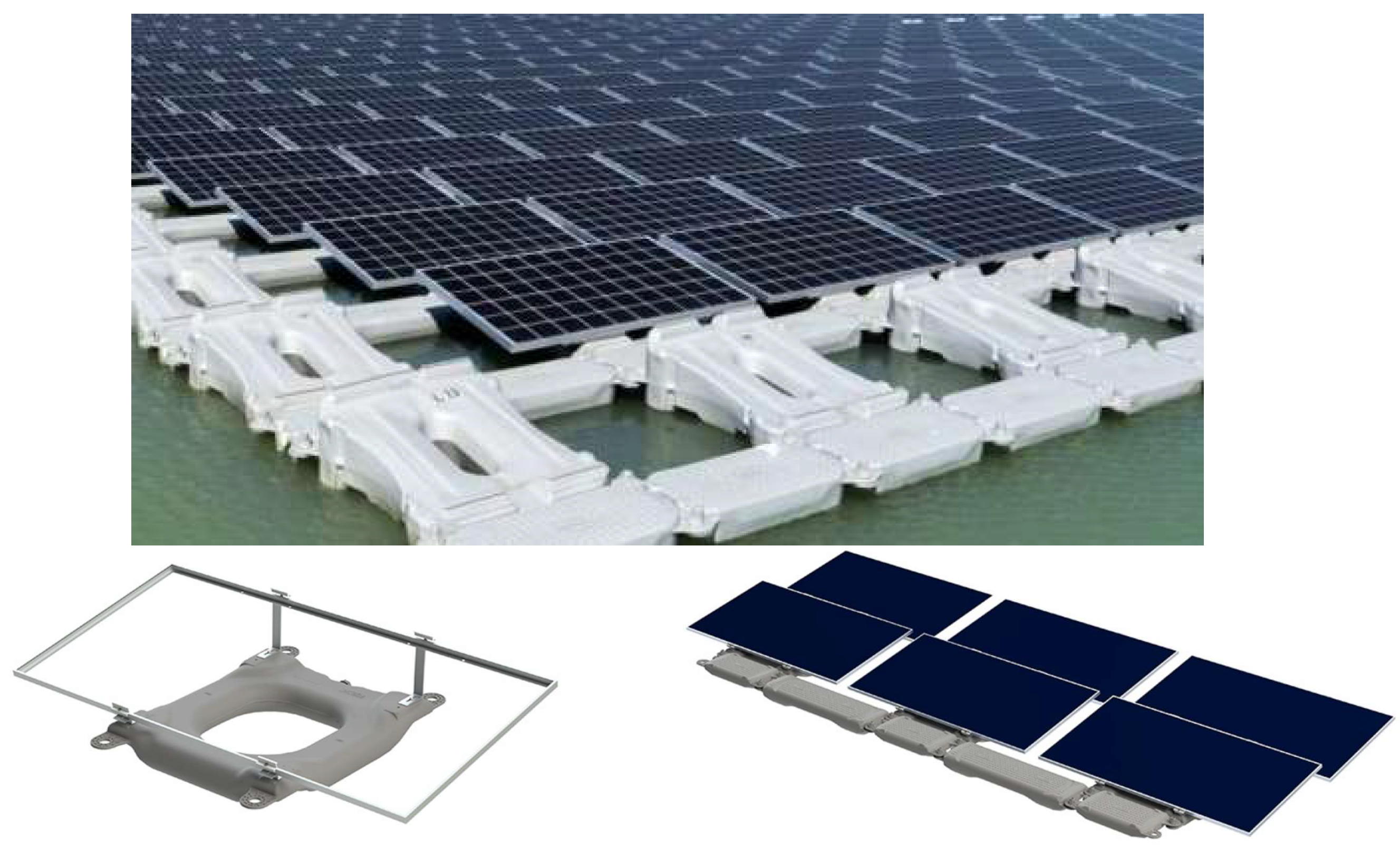
In this study, only the first category is considered, including mono-tilt panels supported by unitary floats (i.e., one float for one PV panel) aligned in parallel rows. Indeed, this type of float arrangement is common among operating FPV farm projects. The chosen float characteristics are adapted from existing cases, although some values were modified for confidentiality reasons. The modelling strategy proposed here could also be used for the second float-type family. The third family requires analysis specific to each individual design.
The PV panels are generic. They are arranged in a landscape position. A 10° inclination angle is considered, as is usually the case to optimize the energy yield and reduce the surface exposed to wind (in Europe for instance). However, the tilt value will not impact the results of this study. The float draft is based on hydrostatic calculations that account for the panel and float weight. As mooring lines are not considered in this study (see Section 3), their weight on the floats is not considered. The geometry is summed up in Table 1 and represented in Figure 1.
2.2. Island Definition
In this article, the proposed floating solar island is composed of unitary floats. To simplify the associated problems, walkways and electrical components were not considered. Mooring was also not considered. These aspects will require inclusion at a later stage; however, this will not change the methodology developed here.
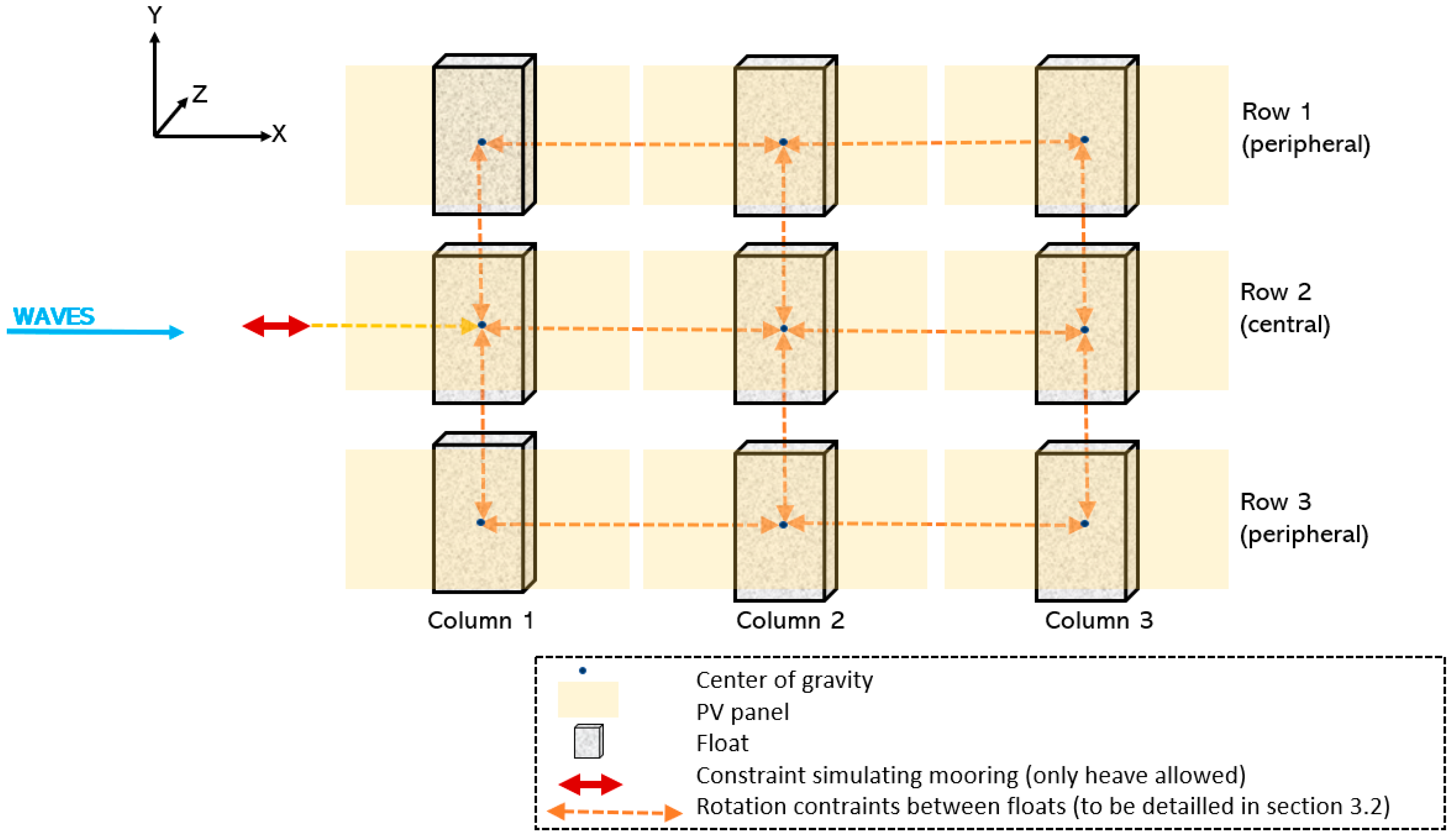
In order to understand the interactions between floats and to limit the computation time, an island composed of nine floats (three rows and three columns) is considered. As illustrated in Figure 2, waves propagate from left to right, along the X-axis. Floats and PV panels are defined as per the properties given in Table 1.
2.3. Environmental Conditions
As the focus of this study is wave-induced dynamic response, the wind and current loads on the FPV island are not included. However, these aspects were studied in [7] using analytical considerations.
The environment is assumed to be a large lake with only wind-generated waves. A rough environment is considered, as it would be considered for mooring design. It should be noted that strong conditions are chosen so that the waves are consistent; however, the waves must not be so strong that the classical multi-float assembly is no longer appropriate. All the environmental conditions are described in Table 2. The waves are calculated based on the available fetch, as per the methodology developed in [7]. Under these conditions, the wavelength is 7.6 m, whereas the spacing between the centres of gravity of the two floats is 2.09 m.
MSL is the mean sea level, Hs is the significant wave height and Tp is the peak wave period. The water level varies for various reasons, such as the following: water extraction and replacement, rainfall patterns, tides, etc. At the preliminary design phase, considering only the mean water level is acceptable. However, at the detailed design phase, water level variation can be a major issue and will need to be considered. It is assumed that these sites are free from extreme weather events, such as typhoons. Environmental conditions are adapted from existing projects, although the data are modified for confidentiality issues. Wind and waves are considered for the ultimate load case, i.e., with a 50-year return period [18]. The wind speed is set as a 10-min wind speed, as is usually the case [7,18]. A Jonswap spectrum is used for the waves, as we are considering a severe environment and it is the most appropriate spectrum [18].
3. OrcaFlex Modelling
OrcaFlex is a commercial software that is commonly used in the offshore industry to perform non-linear time-domain analyses, and to anticipate floating structures’ motions and subsequent loads in the mooring lines.
3.1. Presentation of the Modelled System
As explained in Section 2.2, a 3 × 3 island (composed of nine floats in total) is considered. The OrcaFlex model is based on the following assumptions:
- PV panels are represented by 6D buoys (OrcaFlex objects defined by their mass, volume and inertial properties, with six degrees of freedom).
- Each PV panel is mounted on an individual float.
- No pathway for intervention is considered.
- No electrical component is considered.
- Mooring is not considered. The float ensemble is limited by a constraint that blocks all the motions but heave, which is located upstream of the first row.
- Panels are interconnected by rotation constraints (detailed in Section 3.2).
3.2. Definition of Mechanical Joints between Floats
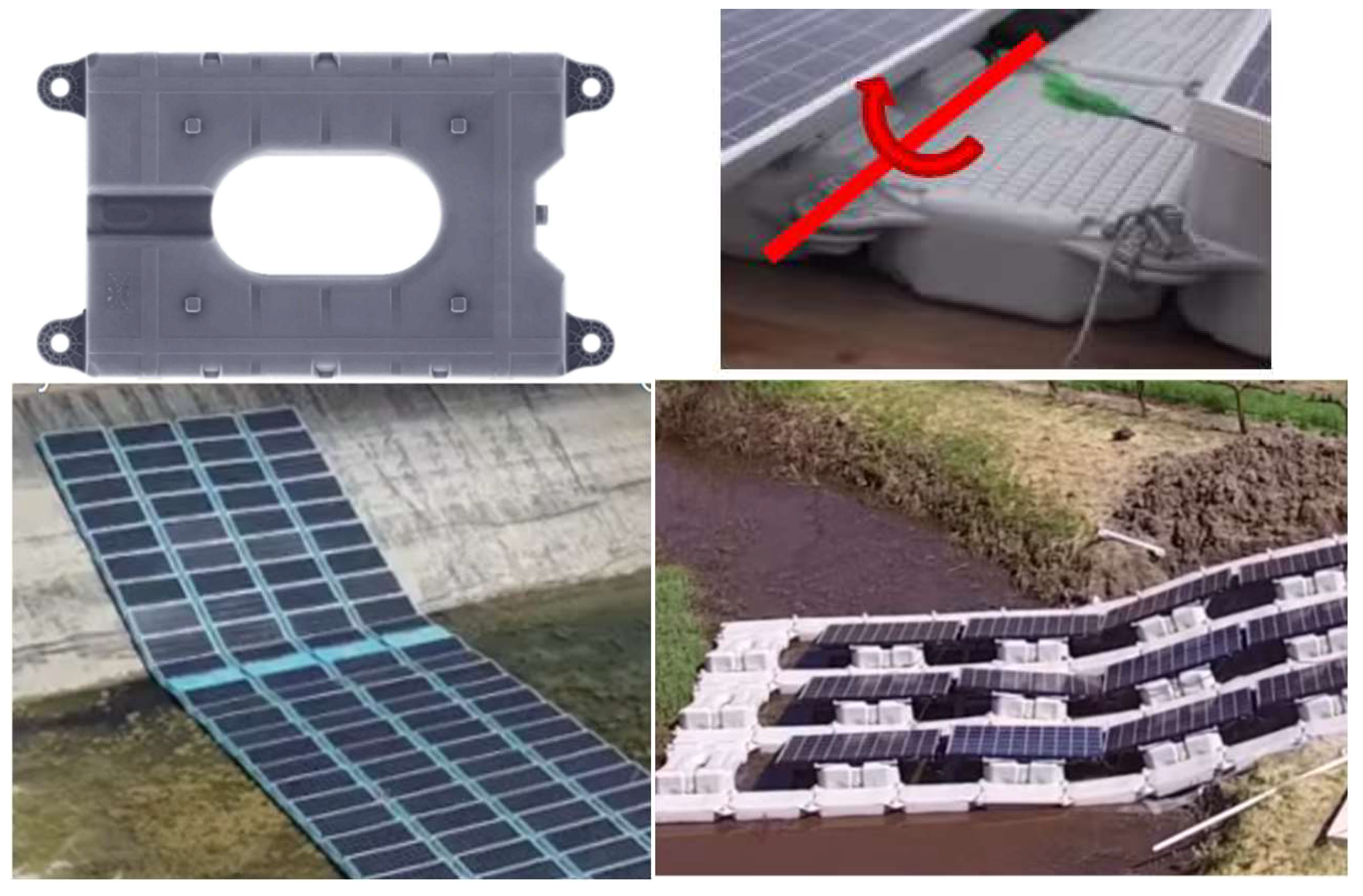
In most cases, floats are connected to one another with two bolted connections to handle waves, soil irregularities in cases of beaching and for deployment (launch ramp). For instance, Ciel & Terre and Isifloating technologies are represented Figure 3.
There is a limit in the admissible angles between the two floats. Based on industrial experience and confidential data from float manufacturers, a 15° limit is considered for this study (i.e., movements allowed in the (−15°; 15°) interval). Several possibilities can be explored to represent inter-float connections. Using only beams or links is not sufficient. Furthermore, it may cause unexpected and unrealistic dynamic behaviour, as can be observed in [15] when using beams. Only the constraints and pivot linkage properly represent the connections and can integrate an angle limit in a straightforward manner. In this study, connections are modelled as the pivot linkage with a 15° limit.
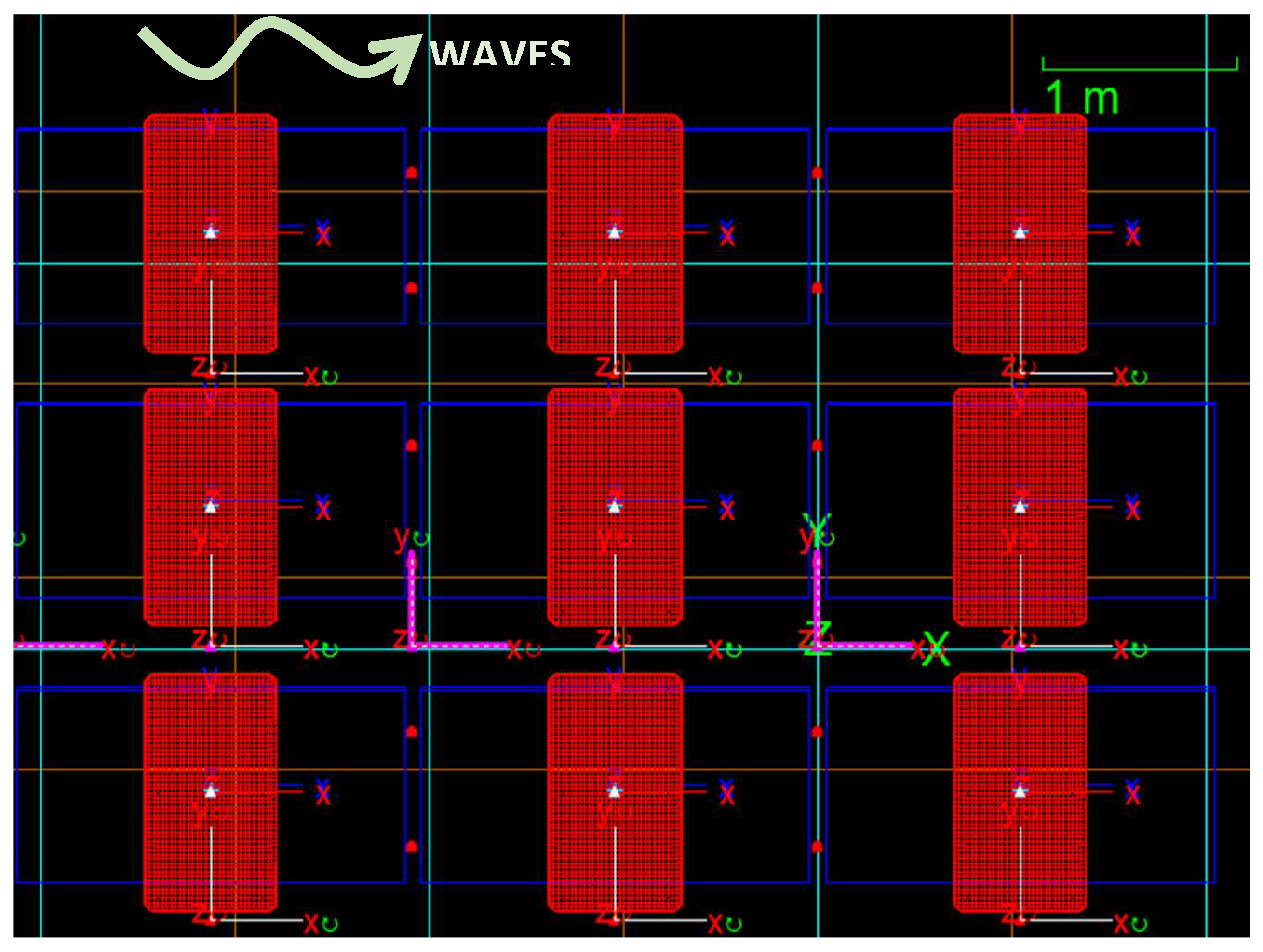
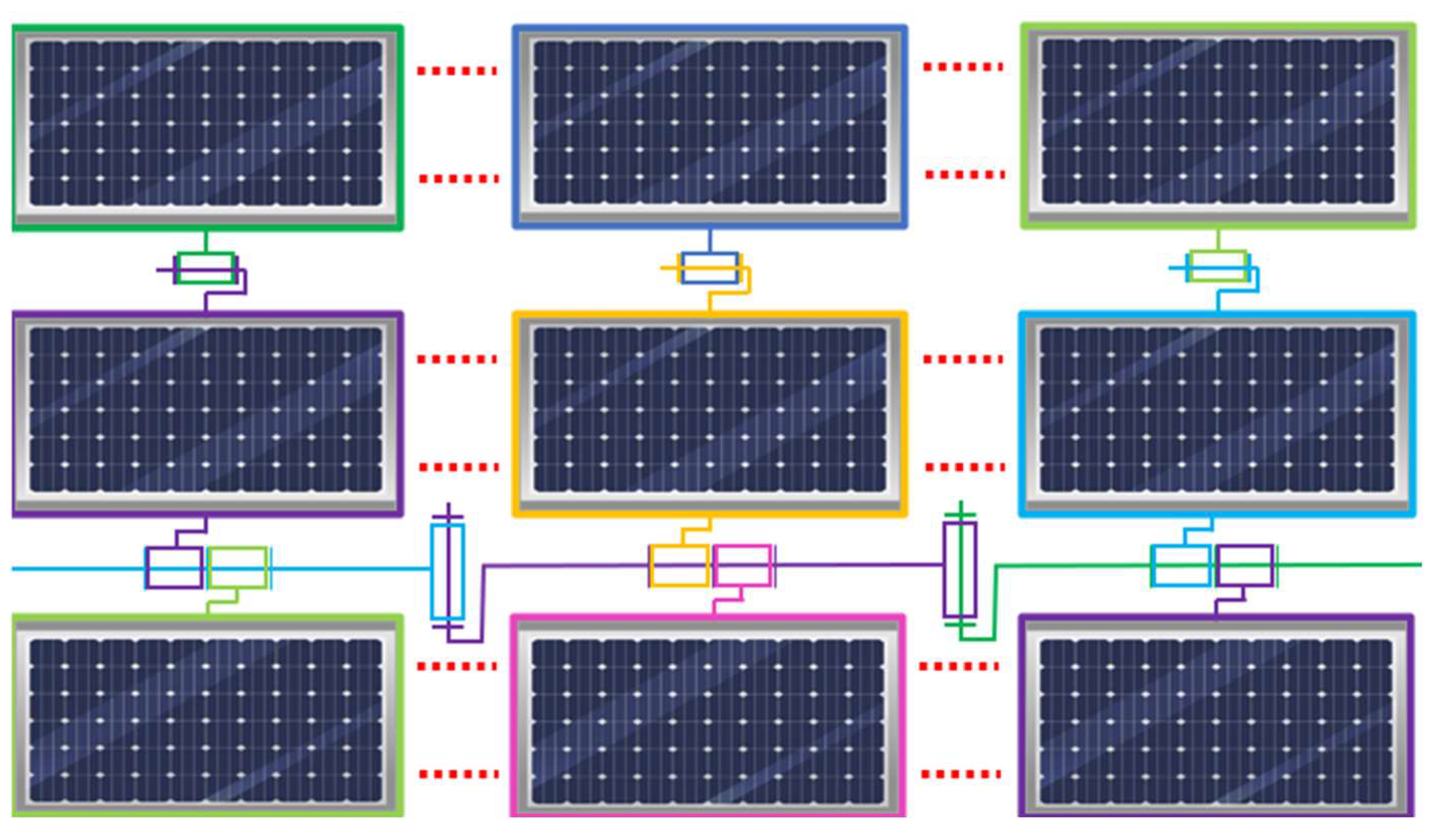
In OrcaFlex, connecting elements with a closed-loop kinematic chain is not possible. To resolve this problem, the kinematic connections in-between floats must be considered at the scale of the whole island, as a kinematic chain of constraints. Eventually, the combination illustrated in Figure 4 and Figure 5 is proposed for the 3 × 3 island (it can be applied to islands of any size, as long as it remains a rectangle).
All the connections represent pivot linkages. All the constraints that limit the rotation around the Y-axis (resp. X-axis) with a 15° limit shall be called Y-constraints (resp. X-constraints).
Between the central row and the lower peripheral row, there is a Y-constraint (Y-constraint-l) and an X-constraint (X-constraint-l). All the Y-constraints-l are connected to one another to form a “constraint chain line”. All the X-constraints-l are connected to the corresponding Y-constraints-l. All the floats in the central row are connected to a X-constraint-l. All the peripherical floats are connected to a new X-constraint, which is connected to the float in the central row. It is not possible to add a new Y-constraint for the peripheral floats, as it would close the kinematic loop, so a solution composed of two springs of quasi-infinite stiffness is proposed (two springs are necessary to insure a pivot linkage). The springs are positioned between floats, on the X-axis. These links are not considered by OrcaFlex as a kinematic constraint, although they provide the same function and solve the problem associated with closed kinematic loops. A schematic representation of the chain of the constraint is shown in Figure 5.
The exact positions and properties of the connections are as follows:
- -
- All the constraints have a 15° limit. In the model, this translates to a connection with no stiffness for an angular displacement lower than 15° and with a quasi-infinite stiffness when the angular displacement exceeds 15°. The 15° limit is imposed gradually to avoid hysteresis movements. Constraints (both X- and Y-constraints) are connected to the floats’ centres of gravity.
- -
- All springs have infinite stiffness. The length of the links is the result of an optimisation between the smallest length and the smallest computation time. Eventually, the best compromise was found to be m. Springs are located at the following positions:
- ∘
- Mid-distance between two floats’ centres of gravity in the horizontal direction.
- ∘
- Mid-distance between the float’s centre and the float’s extremity in the vertical direction (both up and down).
This representation of the chain of constraints accounts for all motions and constraints within a floating solar island. However, it is complex and requires a large number of elements compared to the number of floats. Further works must focus on simplifying this methodology, whilst maintaining realistic interactions between floats.
3.3. Interactions between Waves and Potential Flow Theory
The aim of the study is to propose a method to model FPV multi-body farms using an industry-adapted software, such as OrcaFlex.
In this section, float refers to the float that supports the PV panels (composed of an immersed and not immersed part), body refers to any floating object studied in a fluid–structure interaction (here, it will often refer to the float). Vessels and buoys refer to OrcaFlex systems. Vessels are rigid bodies that are large enough for wave diffraction to be significant. Vessel motions are calculated through diffraction analyses, and then imported into OrcaFlex. Buoys are rigid bodies with both mass and moments of inertia. The corresponding forces and moments are used for Morison’s theory. As opposed to vessels, object motions cannot be applied to buoys.
When studying wave–structure interactions, one must consider radiation and excitation forces. In order to understand the global behaviour of the system and how it interacts with the waves, one must calculate the Keulegan–Carpenter number (KC number). It allows us to estimate the relative importance of drag forces over inertia forces and is defined by the following formula:
where is the maximal amplitude of the flow velocity oscillation, is the period of the oscillation and is the characteristic length of the floating object.
Here and are derived from the wave kinematics and wave period respectively while corresponds to the object length submitted to waves.
is evaluated using Airy wave theory with infinite depth, from which the following relationship may be derived:
There are two possible lengths that can be considered when calculating the KC number and these are as follows: when considering the whole island and m when considering only one float. In the first case, and in the second, . For both cases, the KC number is small (), which suggests that the amplitude of the motion of water particles is relatively small compared to the characteristic length and indicates the predominance of inertial effects over viscous effects [20]. In this case, it is necessary to consider wave excitation forces, which can be divided into the following two categories: Froude–Krylov and diffraction forces. To do so, the linear potential flow solver OrcaWave [21] is used.
Before using OrcaWave, the submerged part on the body (i.e., the part of the body that interacts with the water) is meshed using Ansys software [22].
In OrcaWave, as described in [21], the fluid is assumed to be incompressible, inviscid and irrotational. The fluid velocity is given by , where the velocity potential, , satisfies Laplace’s equation in the fluid domain and boundary conditions on the seabed, on the body surface, and on the free surface.
First-order equations are linear, which allows the expression of as follows:
is the potential of the incident waves, is the scattered potential, and is the radiation potential.
Each component satisfies the boundary value problem that is solved by using Green’s theorem [23]. More details on the resolution of the potential equations can be found in [21].
OrcaWave solves the boundary value problem described above in the frequency domain and yields the velocity potential for all mesh panels. Pressure calculation is performed by means of Bernoulli’s equation, which is as follows:
X is the position of the mesh panel centre and is the time step. The boundary conditions are described accurately in [21]. OrcaWave solves the above-mentioned equations for all the points defined in the mesh. The equations are solved for a range of frequencies that are predefined by the user.
Eventually, OrcaWave calculates the diffraction radiation coefficients that are used in OrcaFlex to solve the Cummins equations in the time domain [24], as shown by the following equation:
M is the mass of the body, is the frequency-dependent added mass, B is the frequency-dependent damping matrix, C is the hydrostatic matrix and is the external forces applied over the body. In this problem, is the Froude–Krylov wave excitation forces. These parameters are outputs of OrcaWave, and they are imported into OrcaFlex in the form of a hydrodynamic database (HDB).
An Implicit scheme (generalized-α integration scheme) is utilized to solve the equation of motion. A constant timestep is used.
OrcaWave also offers the possibility of conducting a multi-body approach. It means that all wave excitation forces in-between floats are accounted for. In this case, the equations detailed in [21] of the radiation potential are extended to the number of bodies. The 15° limit cannot be implemented in OrcaWave; however, this will not be a problem, as the assumption of small float motions is made by the potential flow solver.
The multi-body approach is already used for pontoon interactions in the case of a floating bridge in OrcaFlex modelling, albeit using a different potential flow solver [12].
This approach is the most precise, but the computation time is high for HDB calculations. Furthermore, the number of elements that can be considered in this approach is limited. Indeed, with the means available on standard calculation computers, the number of elements in OrcaWave is limited, and so is the number of floats that can be modelled.
In the case where the KC number is high and viscous effects dominate, only drag forces can be considered. In this case, buoy elements with drag coefficients can be used in OrcaFlex. However, this case is not realistic under the environmental conditions presented in this study, and is thus not considered here.
3.4. Modelling Strategies
The goal is to model a 3 × 3 floating island that is composed of nine floats. In order to assess the methodology that optimises the computation time without compromising the accuracy of the results, different modelling strategies are investigated. They are denoted A, B and R for reference. For all models, floats are modelled with OrcaFlex vessel elements. Each float is represented by a vessel and they are combined together to form the floating island. An HDB is calculated for each float using potential flow theory to account for diffraction–radiation forces (see Section 3.3).
For each modelling strategy, the hydrodynamic and physical interactions between the floats are different. The goal is to compare different refinements of the following models:
- Model A: a single float is considered alone. In this case, the HDB is calculated for a single float and is applied to each float separately. Therefore, all floats behave as if they were alone and hydrodynamic interactions are not considered. It is considered to be a “single-body” approach.
- Model B: a rigid ensemble with all nine floats is considered. It is considered to be a “rigid body” approach.
- Model R: all nine floats are considered in the OrcaWave model and the potential equations are solved for each float individually. Hydrodynamic interactions between the floats are accounted for. It is considered to be a “multi-body” approach.
Afterwards, the HDB is imported into OrcaFlex for the following models:
- For model A: the same HDB is applied to all floats.
- For model B: only one HDB is applied to the rigid 3 × 3 ensemble.
- For model C: an HDB, including different data for each float, is applied to the ensemble.
For each model, the mesh is the same (see Section 3.5); however, meshing is carried out for one or nine floats depending on the modelling strategy. The specificities of each modelling strategy are detailed in Table 3.
As it accounts for most of the physical effects, model R is chosen as the reference model. It is, thus, used as a starting point for modelling strategy optimization. However, this case requires the highest computation time. It should be noted that the goal is to reduce the computation time (or to reduce the refinement of the model), whilst remaining as close as possible to reality. Hence, other methodologies (A and B) will be compared to model R.
3.5. Hydrodynamic Interactions between Floats
Model R is the most refined model and it is considered as a reference in this study. The results for model R are presented in this section.
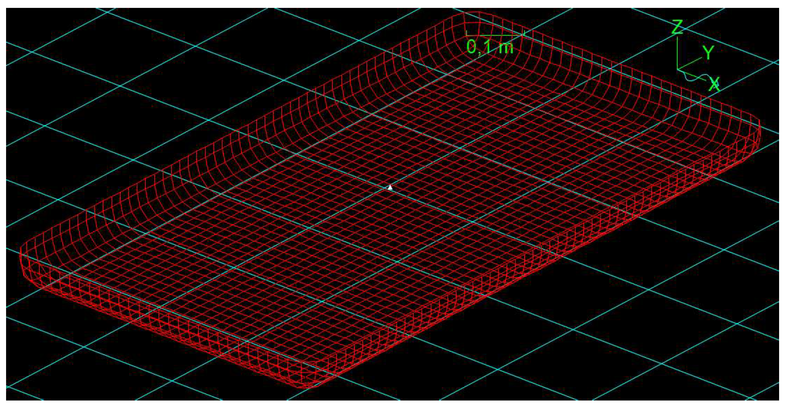
A convergence study concluded that 1948 panel elements are required to mesh each float (see Figure 6). With the computation limitations of our machines, a maximum of 16 floats can be considered. In this study, only nine are considered. Only the submerged part of the float (at equilibrium) is represented in OrcaWave, considering that the submerged volume will not change. This is a valid assumption when considering small motions.
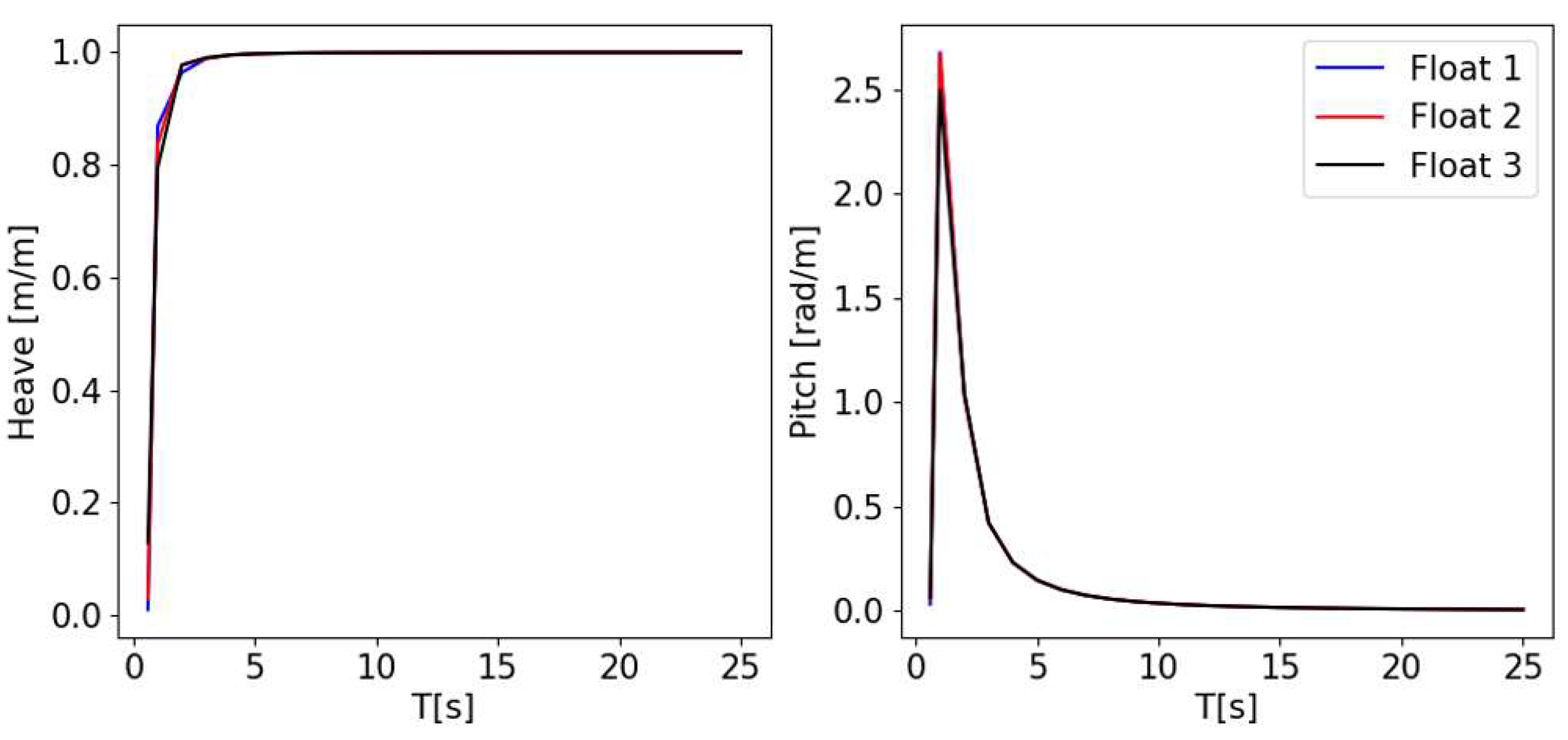
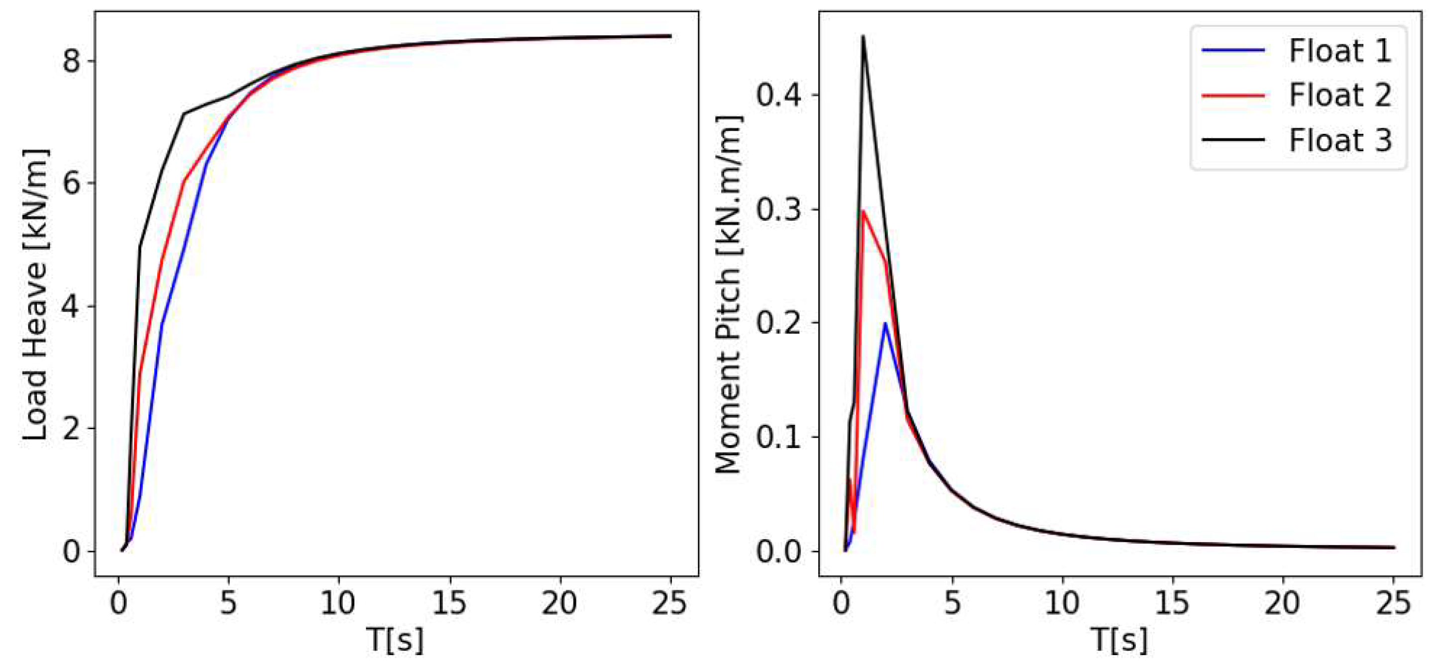
First, RAOs (response amplitude operators) of model R are investigated. The main load and displacement RAOs are depicted in Figure 7 and Figure 8 for the three floats of the central row. Number 1 is the first float impacted by waves and number 3 is the last. Heave is quite similar between all three floats, although pitch is slightly higher for the middle float. Load (and moment) shows great differences. During low periods, float 1 always has the lowest load and moment compared to float 3, which has the highest (almost twice as high). Float 2 stands in-between. During high periods, all three floats stabilise around the same values. Hence, although the motion responses of all the floats are similar, waves will induce forces with a greater magnitude on the last float. It is assumed that this is due to interactions between floats that induce stronger effects on the last float. This illustrates the complexity of hydrodynamic interactions between floats that are only accounted for in the R model (which includes multi-body calculations on OrcaWave).
By definition, potential flow theory does not account for drag. It assumes small motions and that the object is large compared to the waves. The fluid is assumed to be irrotational. Damping is not accounted for neither in the waves’ motions, the floats’ motions, nor the floats’ connections.
For model B, the HDB is calculated for nine floats, rigidly connected (thus considered as one single body) and without the multi-body approach. The mesh for model B is the same as the one presented for case R. For model A, only one float is considered, thus simplifying the process of OrcaWave calculations. The HDB is calculated for the single float and is then applied to all nine floats.
4. Results and CPU Time Optimization
This study focuses on the modelling of the island and the representation of float interactions. It must be noted that the mooring lines and the anchors are not represented, and they will be studied in further works. In this model, the island offsets are simply restricted in surge and sway by a constraint. This simplification is acceptable, as long as mooring is not the topic of the study.
One-hour simulations are performed. The compliance of the seed with the norm [25] is checked in order to ensure that it is representative of the sea state. A timestep of 0.02 s is used, as proposed by OrcaFlex as the optimal timestep for computation. The first 50 s of simulation are not considered for analysis in this section, as they correspond to a transitional phase.
4.1. Results of Regular Waves
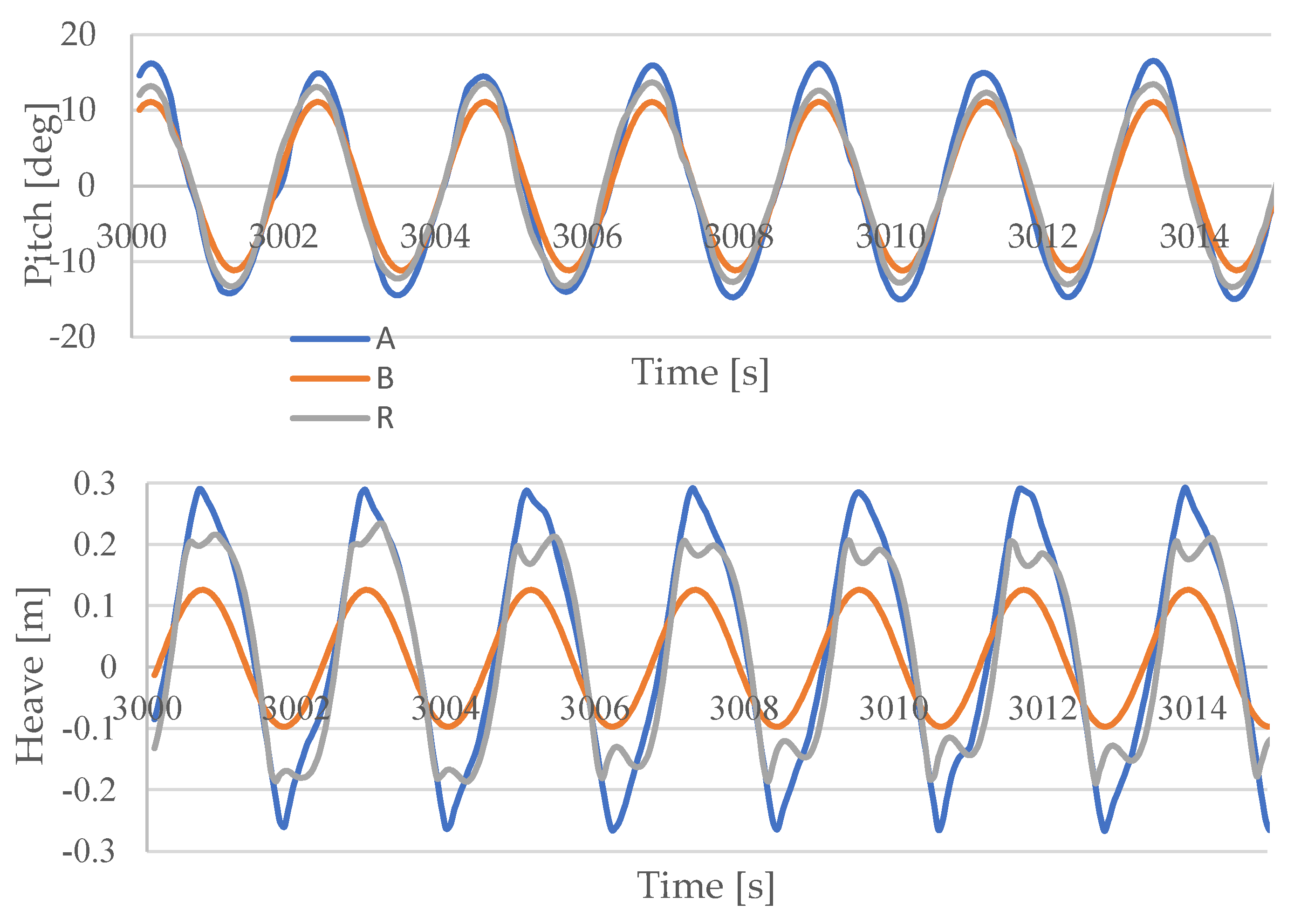
The conditions described in Table 2 are considered, first as a regular Airy wave approximation. This means that the regular waves have the following properties: and The results are presented in Figure 9, Figure 10 and Figure 11 for the central float. All the motions are recorded at the centres of gravity of the floats.
Figure 9 shows that pitch motion is very similar for all models, although model A overestimates the motion amplitude compared to the reference R. Model B underestimates it.
However, heave motions are dissimilar. For these wave conditions, heave motions for model B have the lowest amplitude and it is almost 50% lower than the reference model R, at maximum amplitude. In this case, as all floats are rigidly connected to each other and considering the wave period, when the central float is at the wave trough, the neighbouring floats are at the wave crest (see figure for model B in Table 3). Consequently, the central float stays above the water level, thus reducing the amplitude of heave motions. Similar reasoning is applicable when the central float is at the wave crest. Hence, model B’s amplitude is too low to be realistic. Model A is the closest to reference R. The amplitude and overall behaviour appear to be realistic. The only difference occurs at the amplitude extrema. Model R shows a secondary peak at the wave crest, corresponding to a harmonic, which does not show on model A’s curve. As model A does not account for float interactions, whereas model R does (using the multi-body approach), it is concluded that this secondary peak is due to float interactions. Such periodic movements are very relevant when considering fatigue, for instance, at fairleads.
Pitch amplitude reaches the 15° angle limit between floats, which is an input of the model. If the waves were different in wave period and amplitude, it might have been exceeded, thus underlining the importance of adding an angle limit to such models.
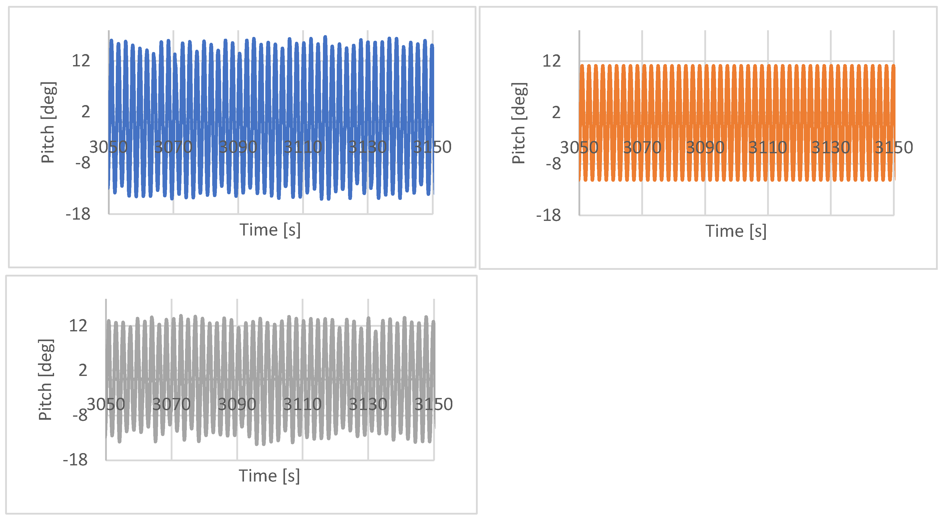
By looking at the pitch signals illustrated Figure 10, a low frequency envelop can be observed. This envelop is present for models R and A and is absent for model B. The hydrodynamic characteristics of model B are different to the reference model. Nonetheless, a frequency analysis must be performed in further works to better understand the hydrodynamic behaviour and differences in the floats’ motions in models R and A.
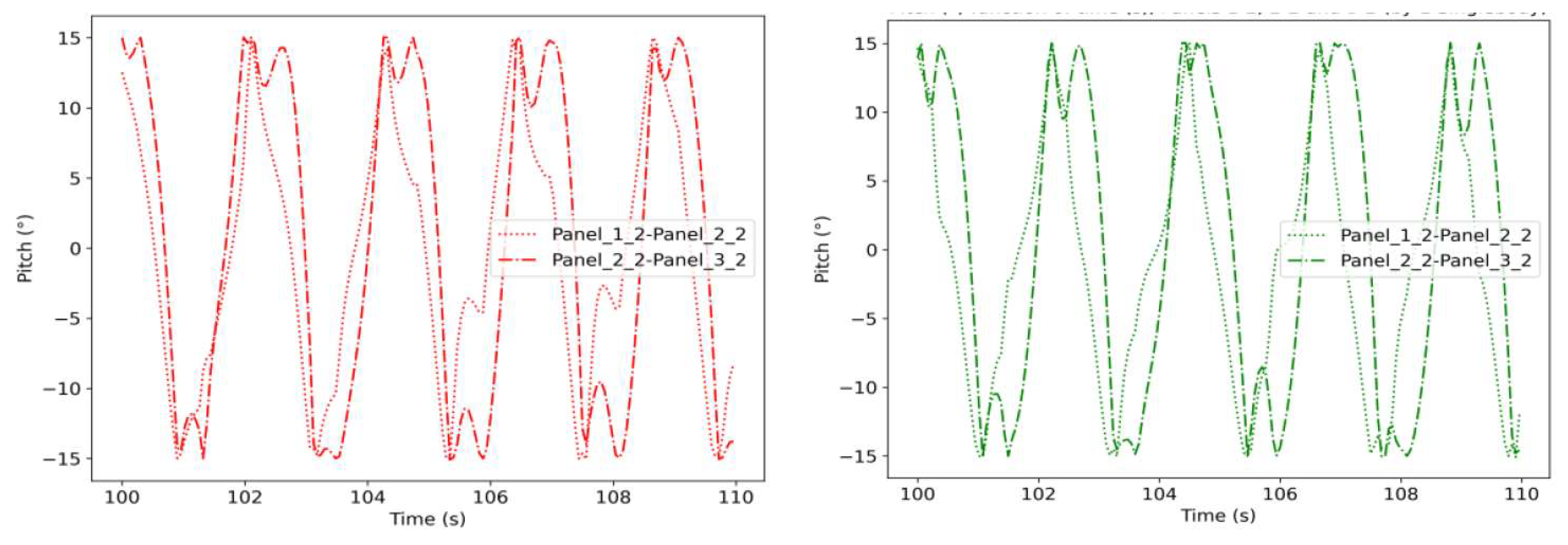
Figure 11 illustrates the relative rotation of each column to the next column. Model B is a rigid ensemble; hence, the motion difference between floats is zero and is not represented here. It is noticed that both graphs show more complex motions between columns 2 and 3 compared to columns 1 and 2, including higher frequency events. This is explained by the fact that column 1 is fixed by a constraint, simulating the mooring.
In order to have a better grasp of the differences between different models, numerical values for heave are summarized in Table 4. They illustrate that the average heave amplitudes are very close for all three models. However, the standard deviation of model A is closer to the reference R (a 16% difference compared to model B, with a 48% difference).
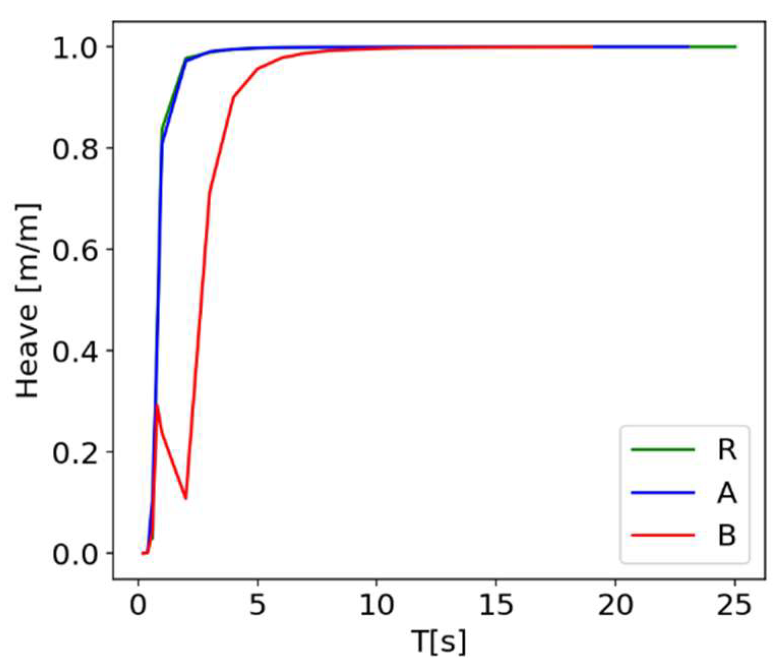
In order to understand the motion differences between all cases, heave RAOs are plotted for the three modelling strategies in Figure 12. All the RAOs are extracted at the centres of gravity of the floats. Similarities between models A and R are clearly illustrated; some small differences are visible for the frequencies between 2 s and 3 s. However, model B is considerably different. It follows the trend of model R up to 0.8 s, then decreases up to 2 s and increases again. This illustrates that model B is not adequate to represent the assembly of a floater, particularly because it is a large rigid body and its natural frequency is not representative.
4.2. Results of Irregular Waves
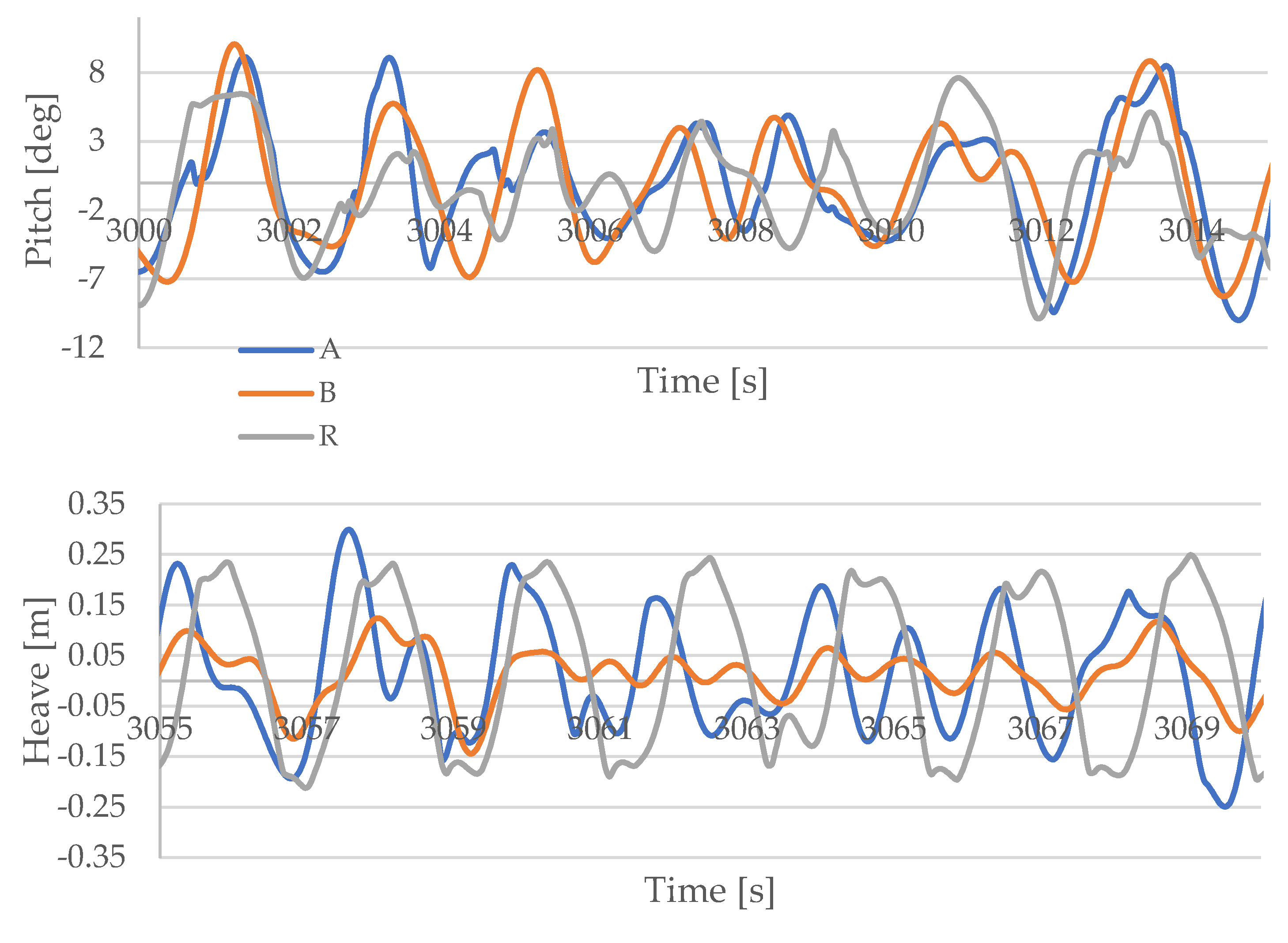
The conditions described in Table 2 are considered for irregular waves. Pitch and heave plots are presented in Figure 13 for all three modelling strategies and for the central float. All the motions are recorded at the centres of gravity of the floats.
In irregular waves, the behaviour differences between all models are heightened. Again, the amplitude of model B motions is lower, especially for heave. Model A is again the closest to the reference, especially for heave. The motions remain higher overall than model R, due to the absence of interactions between floats.
It is worth mentioning that, although model A does not account for all hydrodynamic phenomena, its dynamic is close to the reference model R and its amplitude is larger than model R, ensuring conservative results. This remark is very relevant when considering FPV island design, as using model A rather than model R would save time and ensure conservative results.
The numerical values obtained for heave are summarized in Table 5. As per regular waves, the average heave motion is almost equal between all three cases. Compared to the reference R, the standard deviation is lower for model B and close for model A. However, the difference is 19% in the standard deviation between models A and R and 43% between B and R.
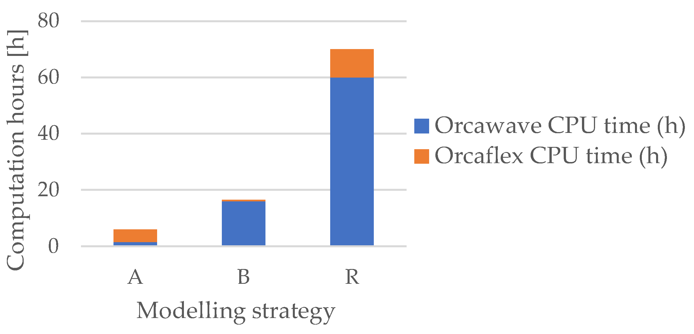
4.3. CPU Time
It has been established at the beginning of this work that the multi-body model is the closest model to reality. However, it is also the most time-consuming. Computation time was recorded for each modelling strategy and presented in Figure 14. It must be kept in mind that these values were used for comparison only and that they vary depending on the computational resource. In addition, this study focuses on one environmental condition only. In reality, we would use the same model for various design load cases. Then, the HDB would have to be calculated only once for all the design load cases. Therefore, modelling strategies such as reference R, which require a long time for HDB calculations but are actually fast on OrcaFlex, would become more advantageous when running a significant number of simulations.
When considering only one simulation, the figure clearly shows that the reference model is up to 3 times more time-consuming than the other strategies. Model A is also two times more effective than model B.
5. Conclusions and Perspectives
In this work, the need for modelling strategies for large multi-body floating islands, using an industry-validated software, is highlighted. Multi-float islands are adapted for sheltered areas, such as lagoons or large lakes, where small waves can occur. In these environments, wave loads, mismatch, fatigue of floats, mooring lines or cables and cable friction can be significant. The non-linear time-domain software OrcaFlex is used in this work. The geometry of one of the most common float types is presented and its dynamic constraints are detailed (connections between floats cannot exceed 15°).
The first challenge presented in this paper deals with the representation on OrcaFlex of the kinematic chain of constraints between floats. It is a complex issue because OrcaFlex cannot deal with the closed loops of constraints. In order to account for all the interactions and to be able to limit the rotation to 15°, a combination of rotation constraints and link elements is considered.
In the environmental conditions chosen in this paper, which are representative of a sheltered area, the float motions are large compared to wave motions, indicating the predominance of inertial effects over viscous effects. In this case, it is necessary to consider wave excitation forces. These forces can be calculated using a potential flow solver, such as OrcaWave. A small 3 × 3 float island is considered at first, to understand how floats interact with each other and which modelling strategy is the most efficient.
Three different modelling strategies are developed, named A, B and R. For model R, the HDB (hydrodynamic database, output of the potential flow solver) is calculated for all nine floats, considering the hydrodynamic interactions between the floats (multi-body approach). This is the most refined model and it is, thus, considered as the reference model. Model A considers one single float for the HDB. The float is considered separately and its HDB is then applied to all nine floats. Model B considers all nine floats, rigidly connected together.
The results show that calculating a HDB for a rigid ensemble underestimates the motions and lacks a large portion of the hydrodynamic content, due to the absence of relative float motions. Modelling strategy A, which uses a HDB that considers each float individually, is effective. It is the least time-consuming strategy and it gives results close to the reference model. There is a 16% difference between models R and A in the heave standard deviation for regular waves and a 19% difference for irregular waves. For model A, float behaviour is close to the reference and motion amplitudes are higher than the reference case. It is, therefore, conservative. However, it does not account for all the harmonic frequencies and lacks the dynamics of float interactions. Nonetheless, it can be considered as a good estimation.
These results are obtained for a specific environmental condition. In order to fully comprehend the behaviour of the system, the model must be run under other environmental conditions and comparisons must be made in further works. Once the model is validated, it can be adapted for a complete mooring design. Mooring lines must be included in the model and full simulations, representative of actual sea states, must be run.
Hence, this paper proposes solutions used to model small-scale floating solar islands. When considering a large-scale island (over 100 floats), the question of the refinement of the model is of high importance. It is possible to consider that, for central floats, waves are dissipated through front float damping. Consequently, the central part of the island can be considered as a large plate. However, for side floats subjected to waves, the model must be refined further and the modelling strategy can be inspired from the work presented in this paper. The refinement of the model, the extension of the present work to larger float assemblies and the representation of multi-float assemblies using flat plates must be investigated in further works. The different strategies and hypotheses presented in this paper must also be validated with in-site or tank measurements.
Author Contributions
Conceptualization, M.I. and B.D.; methodology, M.I. and A.B.; software, A.B. and M.I.; formal analysis, A.B., M.I. and J.-C.G.; investigation, M.I., A.B., B.D. and J.-C.G.; writing—original draft preparation, M.I.; writing—review and editing, J.-C.G.; supervision, J.-C.G. All authors have read and agreed to the published version of the manuscript.
Funding
This research was funded by the INTERREG North-West Europe Marine Energy Alliance project funded under the FEDER program and the TRUST PV project funded by the European Commission under the Horizon 2020 program, under Grant Agreement 952957.
Acknowledgments
The authors are grateful to INNOSEA’s team and especially to Simon Tonnel, Valentin Arramounet and Quentin Trébaol for their advice, guidance and participation in this work.
Conflicts of Interest
The authors declare no conflict of interest.
References
- World Bank Group; ESMAP; SERIS. Where Sun Meets the Water, Floating Solar Market Report; World Bank Group: Washington, DC, USA, 2018. [Google Scholar]
- Perez, M.; Perez, R.; Ferguson, C.R.; Schlemmer, J. Deploying effectively dispatchable PV on reservoirs: Comparing floating PV to other renewable technologies. Sol. Energy 2018, 174, 837–847. [Google Scholar] [CrossRef]
- Claus, R.; López, M. Key issues in the design of floating photovoltaic structures for the marine environment. Renew. Sustain. Energy Rev. 2022, 164, 112502. [Google Scholar] [CrossRef]
- Friel, D.; Karimirad, M.; Whittaker, T.; Doran, W.; Howlin, E. A review of photovoltaic design concepts and installed variations. In Proceedings of the 4th International Conference on Offshore Renewable Energy, Glasgow, UK, 29–30 August 2019. [Google Scholar]
- Sahu, A.; Yadav, N.; Sudhakar, K. Floating photovoltaic power plant: A review. Renew. Sustain. Energy Rev. 2016, 66, 815–824. [Google Scholar] [CrossRef]
- Trapani, K.; Redón Santafé, M. A review of floating photovoltaic installations: 2007–2013. Prog. Photovolt. Res. Appl. 2015, 23, 524–532. [Google Scholar] [CrossRef] [Green Version]
- Ikhennicheu, M.; Danglade, B.; Pascal, R.; Arramounet, V.; Trébaol, Q.; Gorintin, F. Analytical method for loads determination on floating solar farms in three typical environments. Sol. Energy 2021, 219, 34–41. [Google Scholar] [CrossRef]
- [Reportage] Akuo Revient sur les Causes de L’incendie sur sa Centrale Flottante O’MEGA 1. PV Magazine, 28 February 2022.
- OrcaFlex ©, Version 11.0; Orcina: Ulverston, UK.
- Sethuraman, L.; Venugopal, V. Hydrodynamic response of a stepped-spar floating wind turbine: Numerical modelling and tank testing. Renew. Energy 2013, 52, 160–174. [Google Scholar] [CrossRef]
- Viuff, T.; Xiang, X.; Leira, B.; Øiseth, O. Code-to-code verification of end-anchored floating bridge global analysis. In Proceedings of the 37th International Conference on Offshore Mechanics and Arctic Engineering, Madrid, Spain, 17–22 June 2018; pp. 1–9. [Google Scholar]
- Xiang, X.; Viuff TLeira, B.; Øiseth, O. Impact of hydrodynamic interaction between pontoons on global responses of a long floating bridge under wind waves. In Proceedings of the ASME 2018 37th International Conference on Ocean, Offshore and Arctic Engineering, Madrid, Spain, 17–22 June 2018; Volume 7A. [Google Scholar]
- Suzuki, H.; Bhattacharya, B.; Fujikubo, M.; Hudson, D.A.; Riggs, H.R.; Seto, H.; Shin, H.; Shugar, T.A.; Yasuzawa, Y.; Zong, Z. ISSC Committee Vi.2: Very large floating structures. In Proceedings of the 16th International Ship and Offshore Structures Congress, Southampton, UK, 20–25 August 2006. [Google Scholar]
- Sree, D.; Law, A.; Pang, D.; Tan, S.; Wang CKew, J.; Seow, W.; Lim, V. Fluid-structural analysis of modular floating solar farms under wave motion. Sol. Energy 2022, 233, 161–181. [Google Scholar] [CrossRef]
- Song, J.; Kim, J.; Lee, J.; Kim, S.; Chung, W. Dynamic response of multiconnected floating solar panel systems with vertical cylinders. J. Mar. Sci. Eng. 2022, 10, 189. [Google Scholar] [CrossRef]
- Ocean Sun Technology. Available online: https://oceansun.no/ (accessed on 21 April 2022).
- Ciel et Terre Technology. Available online: www.ciel-et-terre.net (accessed on 12 June 2022).
- DNVGL-RP-C205; Environmental Conditions and Environmental Loads. DNV: Høvik, Norway, 2019.
- Isifloating Technology. Available online: www.isifloating.com (accessed on 14 August 2022).
- Molin, B. Hydrodynamique des Structures Offshores; Editions TECHNIP: Paris, France, 2020. [Google Scholar]
- OrcaWave ©, Version 11.0; Orcina: Ulverston, UK.
- Ansys, Version 15; Ansys: Canonsburg, PA, USA.
- Newman, J.N. Algorithms for the free-surface Green function. J. Eng. Math. 1985, 19, 57–67. [Google Scholar] [CrossRef]
- Cummins, W.E. The Impulse Response Function and Ship Motions; Report no. DTMB-1661; Washington, DC, USA, 1962. [Google Scholar]
- DNVGL-RP-0584; Design, Development and Operation of Floating Solar Photovoltaic Systems. DNV: Høvik, Norway, 2021.
Figure 1.
Example of FPV farm (top) and Hydrelio float representation (bottom) by Ciel & Terre [17].
Figure 1.
Example of FPV farm (top) and Hydrelio float representation (bottom) by Ciel & Terre [17].

Figure 2.
Schematic representation of the system modelled.

Figure 3.
Floater assembly and angle limitation for Isifloating [19] (top and bottom left) and Ciel & Terre [17] (top and bottom right) technologies.

Figure 4.
OrcaFlex representation of a 3 × 3 island (top view). Floats are in red and panels are in blue. Waves propagate along the X-axis (from left to right).
Figure 4.
OrcaFlex representation of a 3 × 3 island (top view). Floats are in red and panels are in blue. Waves propagate along the X-axis (from left to right).

Figure 5.
Schematic representation of the chain of constraints on a 3 × 3 island. Red dots represent the pivot linkage (2 parallel springs) and colored boxes are the kinematic constraint pivots. Colors are only used to differentiate the different floats.
Figure 5.
Schematic representation of the chain of constraints on a 3 × 3 island. Red dots represent the pivot linkage (2 parallel springs) and colored boxes are the kinematic constraint pivots. Colors are only used to differentiate the different floats.

Figure 6.
Mesh for one float on OrcaWave.

Figure 7.
Displacement RAOs for floats of the central row: heave (left) and pitch (right) for model R (multi-body approach).
Figure 7.
Displacement RAOs for floats of the central row: heave (left) and pitch (right) for model R (multi-body approach).

Figure 8.
Load RAOs for floats of the central row: heave (left) and pitch (right) for model R (multi-body approach).
Figure 8.
Load RAOs for floats of the central row: heave (left) and pitch (right) for model R (multi-body approach).

Figure 9.
Pitch (top) and heave (bottom) motions on the central float for all 3 modelling strategies in regular waves.
Figure 9.
Pitch (top) and heave (bottom) motions on the central float for all 3 modelling strategies in regular waves.

Figure 10.
Pitch for case A (top left), case B (top right) and case R (bottom) on the central float in regular waves.
Figure 10.
Pitch for case A (top left), case B (top right) and case R (bottom) on the central float in regular waves.

Figure 11.
Relative rotation along Y-axis between each column (P1_2 = relative rotation of column 1 to column 2) for models A (left) and R (right) in regular waves.
Figure 11.
Relative rotation along Y-axis between each column (P1_2 = relative rotation of column 1 to column 2) for models A (left) and R (right) in regular waves.

Figure 12.
Heave RAOs for cases A, B and R for the central floater.

Figure 13.
Pitch (top) and heave (bottom) motions on the central float for all 3 test cases in irregular waves.
Figure 13.
Pitch (top) and heave (bottom) motions on the central float for all 3 test cases in irregular waves.

Figure 14.
Comparison of computation time for all modelling strategies when running one simulation.


Table 1.
Characteristics of a single float and PV panel. (*): spacing between centers of gravity (CoG).
Table 1.
Characteristics of a single float and PV panel. (*): spacing between centers of gravity (CoG).
| Property | Unit | Value |
|---|---|---|
| Float length (x) | (m) | 1.23 |
| Float width (y) | (m) | 0.69 |
| Float height (z) | (m) | 0.40 |
| Float draft | (m) | 0.05 |
| Spacing between floats (x) * | (m) | 2.09 |
| Spacing between floats (y) * | (m) | 1.50 |
| Float mass | (kg) | 16 |
| PV panel mass | (kg) | 30 |
| PV panel tilt | (deg) | 10 |
| PV panel CoG position above water surface | (m) | 0.43 |
Table 2.
Summary of conditions for the environment and the floating island layout. Waves are irregular.
Table 2.
Summary of conditions for the environment and the floating island layout. Waves are irregular.
| Environmental Condition | Unit | Value |
|---|---|---|
| Wind speed | (m/s) | 40 |
| Fetch | (m) | 3000 |
| Water depth MSL | (m) | 90 |
| Wave Hs | (m) | 0.9 |
| Wave Tp | (s) | 2.2 |
Table 3.
Summary of modelling strategies (images for visualisation purpose only).
| Pros | Cons | Example of Behavior in Regular Waves | |
|---|---|---|---|
| Single body-A | Requires very little computation time. | No hydrodynamic interactions between floats. |  |
| Rigid body-B | Very fast OrcaFlex calculations. | No hydrodynamic interactions nor dynamic motions between floats. |  |
| Multi-body-R | Accounts for hydrodynamic interactions between floats. | Requires high computation time. |  |
Table 4.
Mean and standard deviation of heave for all modelling strategies in regular waves.
| R | A | B | |
|---|---|---|---|
| Mean (Z) (m) | 0.442 | 0.449 | 0.441 |
| Std (Z) (m) | 0.152 | 0.176 | 0.079 |
Table 5.
Mean and standard deviation of heave for all modelling strategies in irregular waves.
| R | A | B | |
|---|---|---|---|
| Mean (Z) (m) | 0.443 | 0.443 | 0.444 |
| Std (Z) (m) | 0.107 | 0.127 | 0.061 |
Publisher’s Note: MDPI stays neutral with regard to jurisdictional claims in published maps and institutional affiliations. |
© 2022 by the authors. Licensee MDPI, Basel, Switzerland. This article is an open access article distributed under the terms and conditions of the Creative Commons Attribution (CC BY) license (https://creativecommons.org/licenses/by/4.0/).
Share and Cite
MDPI and ACS Style
Ikhennicheu, M.; Blanc, A.; Danglade, B.; Gilloteaux, J.-C. OrcaFlex Modelling of a Multi-Body Floating Solar Island Subjected to Waves. Energies 2022, 15, 9260. https://0-doi-org.brum.beds.ac.uk/10.3390/en15239260
AMA Style
Ikhennicheu M, Blanc A, Danglade B, Gilloteaux J-C. OrcaFlex Modelling of a Multi-Body Floating Solar Island Subjected to Waves. Energies. 2022; 15(23):9260. https://0-doi-org.brum.beds.ac.uk/10.3390/en15239260
Chicago/Turabian StyleIkhennicheu, Maria, Arthur Blanc, Benoat Danglade, and Jean-Christophe Gilloteaux. 2022. "OrcaFlex Modelling of a Multi-Body Floating Solar Island Subjected to Waves" Energies 15, no. 23: 9260. https://0-doi-org.brum.beds.ac.uk/10.3390/en15239260
Note that from the first issue of 2016, this journal uses article numbers instead of page numbers. See further details here.