Electro-Hydraulic Variable-Speed Drive Networks—Idea, Perspectives, and Energy Saving Potentials

Abstract

Electro-hydraulic differential cylinder drives with variable-speed displacement units as their central transmission element are subject to an increasing focus in both industry and academia. A main reason is the potential for substantial efficiency increases due to avoidance of throttling of the main flows. Research contributions have mainly been focusing on appropriate compensation of volume asymmetry and the development of standalone self-contained and compact solutions, with all necessary functions onboard. However, as many hydraulic actuator systems encompass multiple cylinders, such approaches may not be the most feasible ones with respect to efficiency or commercial feasibility. This article presents the idea of multi-cylinder drives, characterized by electrically and hydraulically interconnected variable-speed displacement units essentially allowing for completely avoiding throttle elements, while allowing for hydraulic and electric power sharing as well as the sharing of auxiliary functions and fluid reservoir. With drive topologies taking offset in communication theory, the concept of electro-hydraulic variable-speed drive networks is introduced. Three different drive networks are designed for an example application, including component sizing and controls in order to demonstrate their potentials. It is found that such drive networks may provide simple physical designs with few building blocks and increased energy efficiencies compared to standalone drives, while exhibiting excellent dynamic properties and control performance.

1. Introduction

The improvement of energy efficiency of hydraulic drives and systems has been a focus of academia and industry for several decades, with this increasing especially within the past 4–5 years. This trend is confirmed by the recent acquisition of Artemis Intelligent Power by Danfoss Power Solutions focusing on digital displacement technology (https://www.danfoss.com/en/about-danfoss/news/dps/danfoss-completes-full-acquisition-of-artemis-intelligent-power/ (accessed on 11 January 2022)), the development of digitally flow controlled multi chamber cylinders by Norrhydro and Volvo Construction (https://www.volvoce.com/global/en/news-and-events/press-releases/2020/pioneering-electro-hydraulic-solution-significantly-improving-fuel-efficiency-in-construction-equipm/ (accessed on 11 January 2022)), the development of variable-speed pump based power units and linear actuators by e.g., Bosch Rexroth (https://apps.boschrexroth.com/rexroth/en/connected-hydraulics/products/cytrobox/ (accessed on 11 January 2022)) (https://apps.boschrexroth.com/rexroth/en/connected-hydraulics/products/cytroforce/ (accessed on 11 January 2022)), the development of efficient floating cup piston pumps and motors by Innas and produced by Bucher Hydraulics (https://www.bucherhydraulics.com/ax (accessed on 11 January 2022)), and so forth. Furthermore, efforts have been placed on the development of hydraulic transformer technology, e.g., the IHT developed by Innas. However, this technology remains to be introduced commercially. Hence, the main current trends are related to either digital hydraulics technology and technology based on variable-speed pumps and motors (henceforward abbreviated variable-speed displacement units).

The field of digital hydraulics has mainly evolved via two paths being digital flow control units and digital displacement units. In both cases, the switching valves and their control play a crucial role for system performance and efficiency [1,2,3,4,5]; however, the energy saving perspectives of digital hydraulics are indeed present and potential application areas broad [6,7,8,9,10,11,12,13,14,15].

Considering drive and systems technology based on variable-speed displacement units, major focus has been placed on their application to differential cylinders for use in both industrial and mobile applications, with special emphasis on standalone cylinder drives, and the handling of the volume asymmetry in various ways. Here, developments encompassing single displacement unit drives [16,17,18,19,20,21,22,23], dual displacement unit drives [24,25,26,27,28,29] and even triple displacement unit drives [30,31,32], all utilizing a single electric motor have been considered. Furthermore, dual displacement unit drives with two motors have also been considered [33,34,35,36,37]. For such drives, the cost of electric components may be considered a challenge for their broad application, and this has been addressed e.g., via component downsizing approaches. These include the use of hydraulic energy storages [38] and the use of valves enabling flow regenerative functionalities [39,40,41,42]. Comprehensive reviews on developments of such types of drives are available in [43,44].

In general, developments have mainly concerned individual standalone electro-hydraulic variable-speed drives, and to a high extent self-contained compact versions with fully enclosed fluid circuits and flexible reservoirs taking only electrical power and control signals as inputs. Hence, their installation and application are somewhat similar to that of linear electro-mechanical linear actuators such as ball screws, spindles etc., however with higher force density, simpler overload protection and resilience to impact loads. Furthermore, similar to electro-mechanical actuators, many developments provide for four quadrant operation, connection to common DC-bus’, and may be equipped with electrical storage devices for increased efficiency. From the perspective of multi-cylinder systems, the main drawbacks with standalone drives are that all functionalities are onboard each drive and that each electric motor must be designed for the maximum power required by the individual cylinder. Hence, in case of a system with n actuators, one basically needs n sets of flexible reservoirs (in case of self-contained solutions), n sets of volume asymmetry compensation mechanisms, n sets of cooling/filtering aggregates, and so forth. Furthermore, auxiliary low power functions are not easily integrated into standalone solutions. Hence, if such functions are required, separate actuation systems need to be installed.

Whereas displacement control at multi-cylinder/motor systems level has been considered for several years [45,46], enabling fairly simple inclusion of valve actuated low power functions, developments extending beyond standalone cylinder drives with variable-speed displacement units have only recently begun to emerge. These may allow both to downsize electric motors and for easy implementation of valves for low power functions. Here, developments include standalone electro-hydraulic variable-speed drives for each cylinder/motor, combined with directional valve connections to common pressure rails (CPR) [47,48,49,50], and variable-speed drives combined with a common supply pump and directional valves [51]. In both cases, control is potentially complicated by the directional valves used.

In many industry segments, current key performance indicators are reliable functionality, cost and efficiency (in that order) (Bosch Rexroth A/S, Denmark). Hence, in order for a broader application of electro-hydraulic variable-speed drive technology, one needs to enable cost reductions, further increased energy efficiency, while reliable functionality obviously is mandatory. Considering the fact that most hydraulic systems include two or more cylinders (or hydraulic motors), it may be appropriate to address these challenges by allowing several cylinders to share reservoir, cooling, filtering, etc., to allow for both electric and hydraulic power sharing and storage, with the functionality realized completely without the use of throttle valves. One approach to realize this is to interconnect hydraulic chambers across cylinders either by variable-speed displacement units or by short-circuiting these, while sharing DC-bus’, essentially constituting networks of variable-speed drives. Such types of drives are proposed in the following, and their design, component sizing, energy efficiencies, and control are considered and exemplified in case studies.

2. The Idea of Electro-Hydraulic Variable-Speed Drive Networks

The idea of electro-hydraulic variable-speed drive networks is inspired by the possibility for not only allowing electric power sharing, but also hydraulic power sharing in electro-hydraulic variable-speed drive systems, and to realize this entirely without conceptual losses (i.e., with losses only related to components). Similar to an electric transformer, a variable-speed displacement unit (VsD) may be considered an electro-hydraulic transformer where the electric motor/drive is the primary side and the hydraulic displacement unit the secondary side. A VsD allows for transforming electric power to hydraulic power and with the appropriate choice of displacement unit, a VsD may operate in four quadrants allowing for passing power back and forth between the primary (electric) and secondary (hydraulic) sides.

The use of four quadrant VsD’s offers the unique possibility to pass flow under pressure between any two chambers, i.e., power can be distributed between any two chambers. Hence, systems with multiple chambers interconnected by VsD’s fed by a common electric DC-bus may ideally allow for improved kinetic energy distribution compared to standalone drive types. However, the possible interconnections may be numerous for a given system, and the most efficient solution may generally not be intuitively clear.

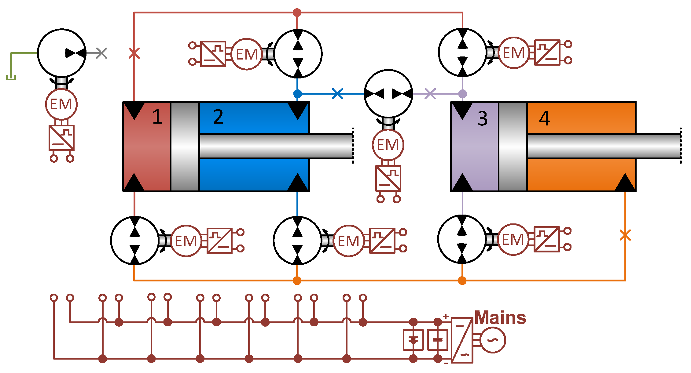
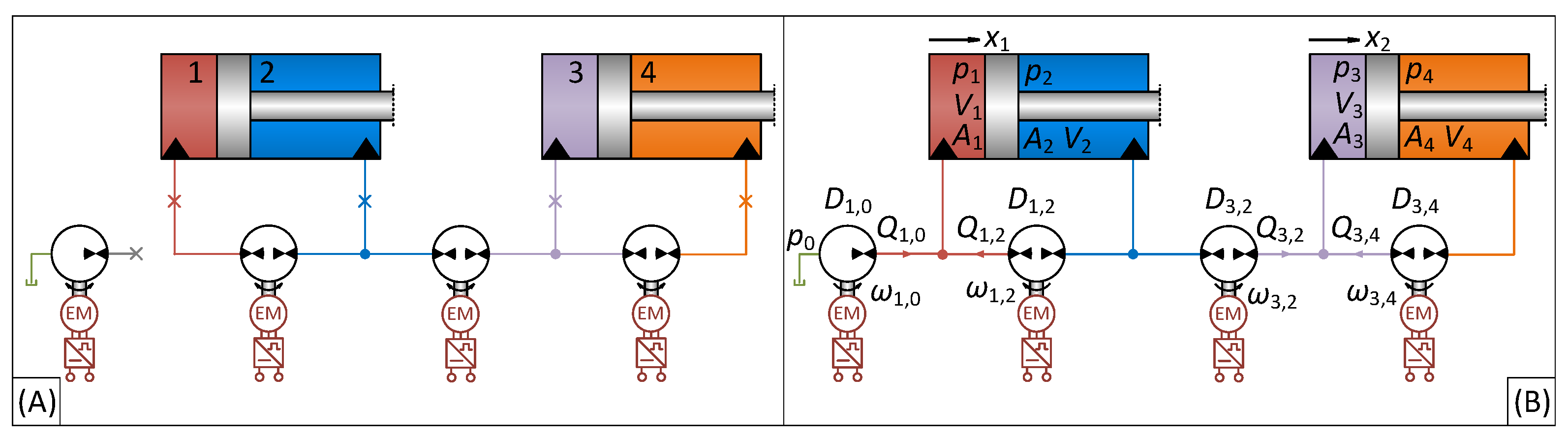
Considering, as an example, the dual cylinder system depicted in Figure 1, any of the cylinder chambers 1, 2, 3, 4 may be interconnected to any other chamber by a VsD. Hence, e.g., chamber 1 may be interconnected to chambers 2, 3, 4, chamber 2 may be interconnected to chambers 1, 3, 4, chamber 3 may be interconnected to chambers 1, 2, 4 and chamber 4 may be interconnected to chambers 1, 2, 3. Noting that, e.g., interconnecting chamber 1 with chamber 4 is the same as interconnecting chamber 4 with chamber 1, the number of chamber interconnections for a dual cylinder system is six. Furthermore, in order to account for volume asymmetry, compression and thermal expansion of the fluid and to accommodate displacement unit drain flows and minor external leakages over cylinder rod seals, at least one VsD should interconnect a chamber to a reservoir, adding at least one additional VsD.

It is notable that electro-hydraulic variable-speed networks (VDN’s) basically can be realized by few building blocks, namely VsD’s, DC-bus’, pipes/hoses, hydraulic cylinders/motors. Furthermore, storage devices (electric batteries/hydraulic accumulators) may allow for further increasing efficiency. These building blocks should be combined in an appropriate manner that enables the desired system functionalities, while controls may realize these functionalities. The strong couplings between the chambers resulting from the interconnections and possible over-actuation entails more complex controls than conventionally used in hydraulic actuator systems. However, with appropriate control designs and a sufficient number of VsD’s, the lower chamber pressure may be controlled to a desired level while controlling motion/forces of the individual cylinders concurrently.

The VDN example illustrated in Figure 1 comprises seven VsD’s in the actuation of only two cylinders. This provides maximum power sharing capability and degrees of freedom in regard to control, but also an excessive amount of VsD’s. Indeed, a main drawback of this example is the cost of realization, especially in relation to the electrical components. However, the potentially high energy efficiency, power distribution ability, few types of building blocks, etc. renders the idea intriguing. From this example, a natural consideration is to what extent the number of VsD’s can be reduced. This opens up a large number of possible topologies and ways to interconnect chambers.

2.1. Classification of VDN Topologies

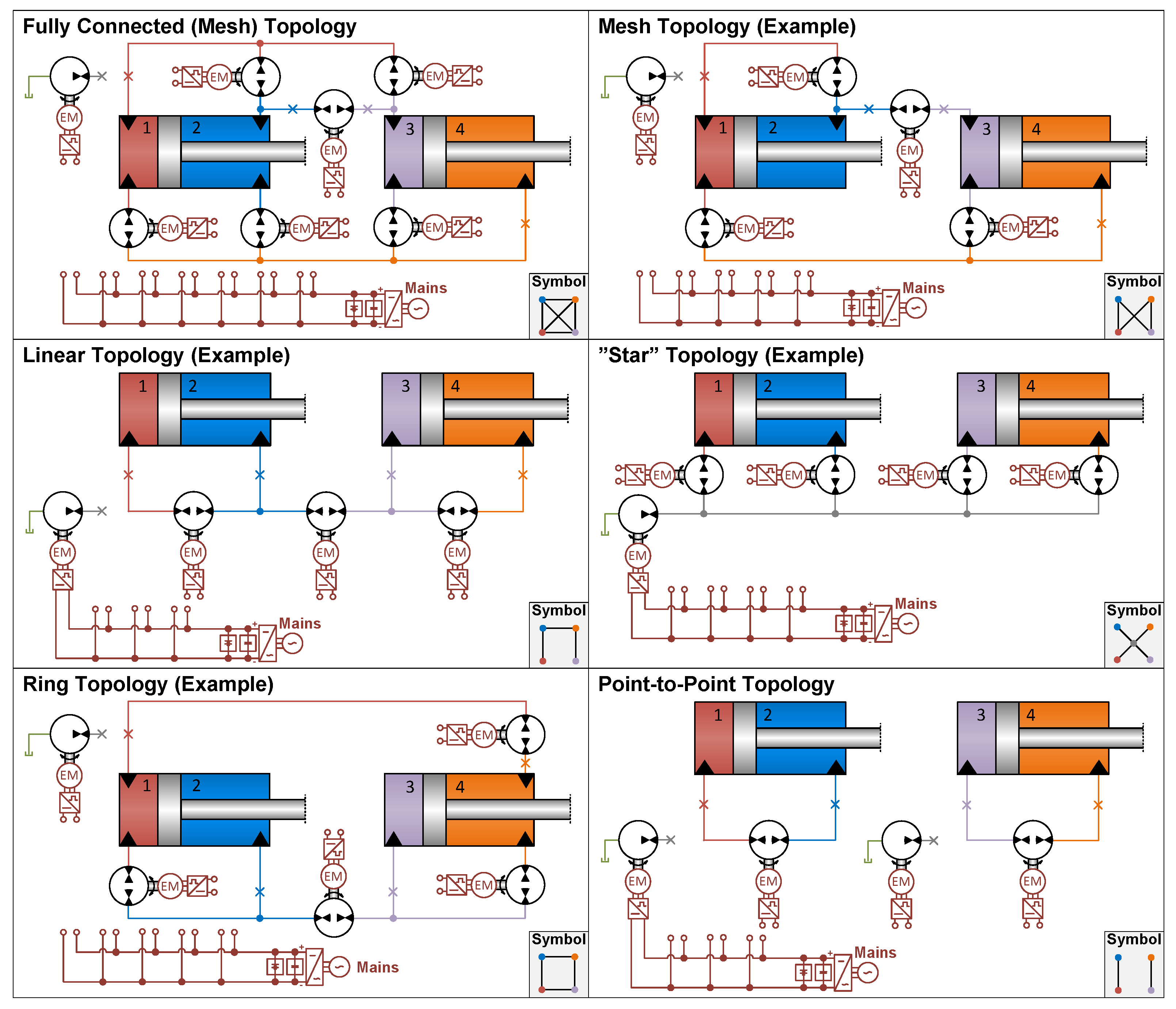
Evidently, a high number of possible VDN topologies may exist for any system containing two or more cylinders/motors. The following aims to classify types of VDN topologies, exemplified with a dual cylinder system; however, the classification also applies to systems with an arbitrary number of cylinders/motors. Even for a dual cylinder system, there exists a significant number of potential VDN topologies, i.e., topologies related to the hydraulic side. To aid the classification of topologies, consider the classification from data communication network theory illustrated in Figure 2 inspired by [52], (https://www.certiology.com/computing/computer-networking/network-topology.html (accessed on 11 January 2022)).

In Figure 2, the devices (computers) are referred to as nodes, whereas the lines/branches are links allowing data communication. Adopting this terminology, the corresponding VDN topologies may be depicted as in Figure 3. Here, hydraulic chambers/lines are the nodes instead of computers/devices, and VsD’s plus adjacent lines are the branches, transmitting power instead of data.

Indeed, the majority of the VDN topologies illustrated in Figure 3 is only examples, as these may be realized in numerous ways, i.e., with many different interconnection schemes. The main features of the individual topologies are considered in the following.

2.1.1. Fully Connected VDN Topology (VDN-F)

The fully connected VDN topology (VDN-F), which is coincident with the example in Figure 1, is essentially a mesh interconnecting all hydraulic chambers via VsD’s. Hence, hydraulic power may be guided from any chamber to another as desired, but also requires six VsD’s for a dual cylinder system plus an additional VsD connected to a reservoir to account for the asymmetric volume flows, fluid compression, thermal fluid expansion, drain flows, and cylinder rod seal leakages. Furthermore, the tank interconnecting VsD may be connected to each of the hydraulic lines. Indeed, the high degree of flexibility of the topology also comes with a high cost related to the large amount of VsD’s used. Furthermore, the seven control inputs cause this to be over-actuated dependent on the number of control objectives, consequently adding significant complexity to the control design.

2.1.2. Mesh VDN Topology (VDN-M)

The mesh network topology (VDN-M) is similar to the fully connected topology, with the difference that not all individual chambers are connected to all other chambers. Hence, mesh topologies allow for guiding hydraulic power from any one chamber to some of the other chambers, but not all of them. Hence, feasible mesh topologies strongly depend on the specific application and the power requirements locally in the system. As may be evident, there exist numerous possible interconnection schemes that may be classified as mesh topologies. Furthermore, the number of control inputs would generally render the system over-actuated, complicating the control design process.

2.1.3. Linear VDN Topology (VDN-L)

A linear network topology (VDN-L) is interconnecting one chamber to a second chamber, the second chamber to a third chamber and so forth, in a bus-like manner. Similar to the mesh topology, there exist several interconnection schemes depending on the order in which the lines are chosen to succeed each other. As opposed to the fully connected and mesh topologies, the number of VsD’s equals the number of chambers, when taking into account the VsD interconnecting the system to the reservoir. Hence, if the motion/force and the pressure levels of the actuators are the control objectives, the system is not over-actuated, simplifying the control design process significantly.

2.1.4. Star VDN Topology (VDN-S)

The start topology (VDN-S) is somewhat similar to a more conventional hydraulic power distribution system. In the event that VsD’s are connecting the chambers to the tank interconnecting VsD, a conventional-like hydraulic power supply would be achieved. However, in such a case, energy regeneration directly between chambers will not be possible. Control design for this topology is not straightforward, as there are more inputs than forces/motions and pressure levels to be controlled.

2.1.5. Ring VDN Topology (VDN-R)

The ring topology (VDN-R) is similar to the linear topology with the only difference that an additional VsD is applied to interconnect the end point chambers. This topology enables the possibility for a controlled fluid circulation between the chamber connecting lines and the reservoir, while concurrently controlling the pressure level and piston forces/motion. The fluid exchange rate depends on pipe/hose lengths and physical connection points. Hence, if fluid exchange is a control objective similar to the actuator motion/force and lower pressure level, such a system is not to be considered over-actuated. In addition, similar to the linear and mesh topologies, several interconnection schemes exist.

2.1.6. Point-to-Point VDN Topology (VDN-PP)

The point-to-point topology (VDN-PP) was already introduced for more than two decades ago, and its control and different applications investigated in [34,53,54,55,56,57]. This topology includes pairwise interconnected VsD’s, and with the individual actuator control objectives defined as e.g., force/motion and the lower pressure at cylinder levels, the control design is fairly straightforward.

2.1.7. VDN Topologies with Shared Actuator Chambers

Indeed, several of the topologies above utilize a high number of VsD’s, potentially causing these to be commercially infeasible, at least with current cost levels on electric components and if axial piston units are preferred over e.g., external gear units. However, the number of VsD’s may be reduced in the event that chambers can be shared/short circuited, as exemplified in Figure 4. The successful realization of such VDN’s strongly depends on the specific application, but renders these physically simpler and potentially more commercially feasible. In addition, the losses may be reduced due to the reduced level of loss mechanisms.

3. Design Considerations and Perspectives of VDN Technology

The perspectives of VDN technology are believed by the authors to be substantial. These include their potential significance in the ongoing electrification and e-mobility transformation in various industries and in relation to trends like Industry 4.0 including condition monitoring, prognosis, and predictive maintenance. That being mentioned, achieving a feasible VDN design with regard to energy efficiency and commercial aspects (component sizes and number of components) may not be straightforward. These considerations and perspectives are discussed in the following.

3.1. Design Aspects

Selection of Feasible Interconnection Schemes As may be evident, the most feasible topology and especially the most feasible interconnection scheme for a given system may not be intuitively clear. Whereas this may be analyzed for dual cylinder systems with reasonable efforts when the load is known (as will be exemplified in Section 4), the related efforts required for systems with three or more actuators may generally be significant. Hence, the development and utilization of optimization routines may greatly reduce the efforts required for these tasks. Furthermore, in case of existing machines, intelligent design methods based on e.g., machine learning methods and online access to the machines states such as pressures, speeds, positions, etc., may aid the topology and interconnections scheme design process, including component sizing.

Integration of Hydraulic Energy Storages Indeed, the loss mechanisms of VsD’s are subject to the main VDN losses. Hence, the efficiency of VDN’s may be increased further by reducing the conversion losses, i.e., limiting the necessity for converting hydraulic power to electric power during operation. This may be achieved by integration of hydraulic accumulators where this is sensible. If one or more cylinders/motors in a system is/are subject to two quadrant operation, one or more chamber pressures may be kept a lower pressure level. If these furthermore are connected to an accumulator, hydraulic power entering these chambers may be converted to potential hydraulic energy in the accumulator. Even though this process is subject to losses, these may generally be considered significantly lower than the conversion losses of VsD’s. Doing so may also allow for downsizing VsD components.

Drive Compactness The approach of entirely avoiding throttle valves possesses some interesting perspectives. The lack of throttle control of the main flows by e.g., proportional valves with large pressure drops over valve control lands reduces the formation of air bubbles in the fluid substantially and hence the requirements for de-gasification of the fluid at the reservoir level. Hence, the necessary period for fluid relaxation and de-gasification is ideally zero. However, VsD leakage flows may be subject to large pressure drops which should be taken into account. Compared to valve controlled systems where all flow is throttled, VsD leakages in VDN’s are limited to a few percentages of the total system flow. Hence, conventional tank solutions may be applied including conventional cooling and filtration methods, however with volumes amounting only to the total rod volumes of cylinders plus some percentages to account for de-gasification of throttled leakage flows, fluid compression, thermal fluid expansion and minor cylinder rod seal leakages. The resulting tank volume requirements will generally be dramatically reduced, substantially increasing system compactness and system level power density. In addition, the potentially highly increased system compactness may allow for installation in close proximity of the machine to be actuated, eliminating potentially long fluid lines, the necessity for dedicated factory space for large decentralized hydraulic power units, etc. In the event of using accumulators as reservoirs, carefully conducted de-gasification procedures should be undertaken similar to existing commercially available self-contained standalone variable-speed drives.

Control Design While it may be evident that VDN architectures should enable a desired system functionality, the VDN controls should enable the functionality. This is not different from many other drive solutions, but the tight hydraulic couplings between the chambers in most VDN topologies/interconnection schemes do not allow common single axis controls. Hence, the controls need to be considered at a systems level. One approach is to consider multi-input-multi-output control structures, including e.g., physically motivated input/output transformation methods combined with single output control methods for motion/force/pressure level control, etc.

3.2. Electrification and E-Mobility Transformation

The electrification and E-mobility trends are rapidly expanding in these years. Due to the inherent electrical interfaces, VDN’s are obvious candidates to bring into play in electrified machinery similar to existing standalone electro-hydraulic actuators based on variable-speed drives. Considering E-mobility applications in terms of mobile machinery such as construction machines and so forth, the up-time of battery powered electric machines naturally depend strongly on their loss levels. The energy saving potentials of VDN’s may play an important role in reducing losses of such machines, and furthermore cleverly engineered interconnection schemes may allow for integrating not only the working hydraulics but also the vehicle transmission.

3.3. Condition Monitoring, Prognosis, Digital Twins, and Predictive Maintenance

Condition monitoring, digital twins, machine prognostics, and predictive maintenance are also areas for which VDN’s may be especially suitable. The reason for this is the few component types used, i.e., VsD’s, DC-bus’, hydraulic cylinders/motors, and potentially electric and hydraulic storage, rendering VDN’s physically simple. This significantly limits the types of potential component failures, as well as the types of uncertainties. As VsD’s basically are the only active components, the main failure critical parameters related to the systems function, besides external leakage, are displacement unit leakages, displacement unit friction, and fluid properties such as viscosity, etc. Generally, a large amount of information about the electric motor, inverter parameters and states may be acquired online, which may be valuable for condition monitoring, etc. In addition, VDN functionalities will generally rely on rather sophisticated controls from which much system information can be extracted online. Hence, when combined with pressure measurements, cylinder positions, etc., solid foundations for the development of online monitoring methods, etc., are present. Such functionalities may indeed allow for the realization of machine prognosis tools, digital twin functionalities and to carry out maintenance when necessary, rather than being based on a maintenance schedule.

4. Case Study on VDN’s Used in Crane Application

It may be difficult to gain an overview of how to choose the most feasible interconnection scheme for a given VDN topology, how to size components, conduct the control design, and the influence on the amount of power to be installed, energy efficiency and power consumption for a given application. Hence, the following aims to exemplify this for a dual cylinder crane application, considering three basic VDN topologies (without the use of hydraulic storages), namely the point-to-point topology (VDN-PP), linear topology (VDN-L) and the linear topology with shared chambers (VDN-LS).

The crane application in consideration is illustrated in Figure 5. Detailed information on the crane modeling, dimensions, mass properties, etc. may be found in [31].

The purpose of the case study is to illustrate possible design and control approaches and to demonstrate the energy saving potential of VDN’s. Hence, it is assumed that all possible component sizes may be chosen, i.e., that arbitrary sizes of hydraulic displacement units, electric motors and inverters can be chosen. Furthermore, the case study is subject to the following constraints and limitations:

• Hydraulic displacement units; The type of displacement unit considered in all cases is the Bosch Rexroth A4FM fixed displacement hydraulic motor that allows operation in all four quadrants.
• Electric motors; The electric motor type considered in all cases is the water cooled Bosch Rexroth MS2N permanent magnet synchronous machine (PMSM). Even though potentially conservative, in the following, a given maximum torque suggested by the displacement unit sizing is chosen as the nominal torque, when choosing the motor.
• Electric inverters; The losses of the inverter may be difficult to estimate in a reliable way similar to the electric motor and hydraulic displacement unit, and, for this reason, a reference loss model of an electric variable frequency drive proposed in [58] is used.
• Electric motor and inverter dynamics; Electric motor and inverter dynamics are excluded in the following, as industry grade components (which are considered here) generally are appropriately controlled with closed loop bandwidths generally comfortably above dominant frequencies of crane dynamics.
• Safety functions, fluid cooling and filtration; VDN’s, as all other hydraulic systems, should encompass safety components limiting pressures in terms of relief and anti-cavitation valves. These are, however, left out in the following, as these are not active in nominal operation. Furthermore, fluid cooling and filtration may be implemented offline at a tank/reservoir level similar to conventional systems, and for this reason left out in the following.

4.1. Design Specification and Commercial Feasibility Considerations for Crane Drive

Even though focus on energy efficiency is increasing, cost remains to be of main significance for obvious reasons. The main costs are related to component types and sizes, but to a high degree also component integration, i.e., the number of components to be built into hydraulic manifolds, electric cabinets, structural machine frames, the amount of working hours required to build a given system, and so forth. Hence, the VDN designs considered in the following aim to realize the crane drive functionality with the least possible amount of displacement and amount of electric motor torque, with the latter prioritized over the former due to their generally higher cost in comparison. Furthermore, the designs aim to satisfy the following overall specifications:

• Maximum piston speeds of $|{\dot{x}}_{1,\max }|=|{\dot{x}}_{2,\max }|=|{\dot{x}}_{\max }|=50$ mm/s.
• Maximum VsD shaft speeds of $|{\omega }_{\max }|=3000$ rpm.
• A minimum chamber pressure of $p_{\min }=20$ bar.

In addition, the loss mechanisms are based on those of existing components, and scaled accordingly by appropriate scaling laws.

4.2. Main VsD Losses

The main losses of a VsD are related to those of the hydraulic displacement unit, the electric motor and the inverter. Detailed steady state losses of these components are modeled in the following, including considerations on the scaling of losses to appropriate component sizes.

4.2.1. Hydraulic Displacement Unit Loss Model

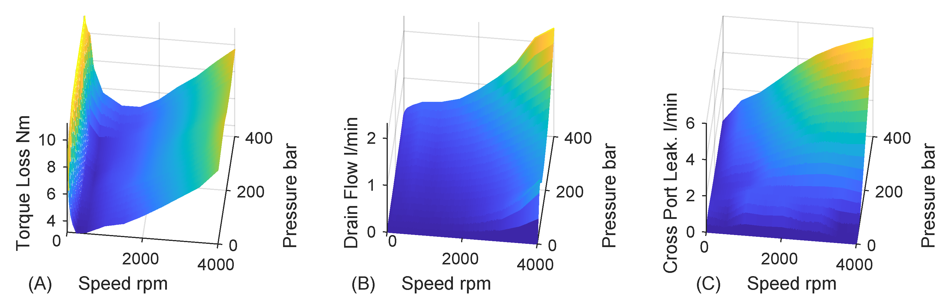
As mentioned above, the displacement unit loss model is based on the Bosch Rexroth A4FM fixed displacement axial piston motor. The associated loss model is based on the leakage, torque loss and total loss measurements of an A4FM unit with a theoretical displacement of $D_{\mathrm{A}4\mathrm{FM}}=27.75$ ccm, presented in [59]. It is thus assumed that a drain flow is present via both displacement unit ports, i.e., that there is a drain flow from the pressurized ports through the housing to the drain line. In addition, it is assumed that the drain line is checked, such that only a drain line flow out of the displacement unit can take place. Based on measurements, approximations of the torque loss, drain flow, and cross port leakage flow (port 1 ↔ port 2) as functions of pressure and speed appear are depicted in Figure 6.

The scaling laws [17] given by Equation (1) are used to scale the reference displacement unit friction torque ${\tau }_{\mathrm{F},\mathrm{ref}}$, the drain flow $Q_{\mathrm{Ld},\mathrm{ref}}$, and the cross-port leakage flow $Q_{\mathrm{Lc},\mathrm{ref}}$ to other displacement unit sizes, where $D_{\mathrm{ref}}=D_{\mathrm{A}4\mathrm{FM}}$ in this case:

$$\begin{array}{cc}\hfill {\tau }_{\mathrm{F}}& =\frac{D}{D_{\mathrm{ref}}}{\tau }_{\mathrm{F},\mathrm{ref}},Q_{\mathrm{Ld}}={\left(\frac{D}{D_{\mathrm{ref}}}\right)}^{\frac{2}{3}}{Q}_{\mathrm{Ld},\mathrm{ref}},Q_{\mathrm{Lc}}={\left(\frac{D}{D_{\mathrm{ref}}}\right)}^{\frac{2}{3}}{Q}_{\mathrm{Lc},\mathrm{ref}}\hfill \end{array}$$

(1)

4.2.2. Electric Motor and Inverter Loss Models

The main losses of an electric motor are associated with its copper and core losses. The electric motor loss model is based on the water cooled versions of the Bosch Rexroth MS2N series, as mentioned above. The copper loss $P_{\mathrm{cu}}$ for a controlled PMSM, not in field weakening, may be described by Equation (2), where $R_{\mathrm{s}}$, $p_{\mathrm{b}}$, $K_{\tau }$, $i_{\mathrm{s}}$, ${\tau }_{\mathrm{L}}$ are the stator resistance, number of pole pairs, torque constant, stator current and load torque, respectively:

$$\begin{array}{cc}\hfill P_{\mathrm{cu}}& =\frac{3}{2}{R}_{\mathrm{s}}{i}_{\mathrm{s}}^2,i_{\mathrm{s}}=\frac{2}{3}\frac{1}{p_{\mathrm{b}}{\Psi }_{\mathrm{m}}}{\tau }_{\mathrm{L}},{\Psi }_{\mathrm{m}}=\frac{2}{3}\frac{K_{\tau }}{p_{\mathrm{b}}}\Rightarrow P_{\mathrm{cu}}=K_{\mathrm{cu}}{\tau }_{\mathrm{L}}^2,K_{\mathrm{cu}}=\frac{3}{2}\frac{R_{\mathrm{s}}}{K_{\tau }^2}\hfill \end{array}$$

(2)

The relation between the core loss $P_{\mathrm{core}}$ and the rotor speed may be approximated by the proportionality $P_{\mathrm{core}}\sim {\omega }_{\mathrm{m}}^{3/2}$ [60]. In addition, the core loss magnitude may be described by some scalar ${\epsilon }_{\mathrm{c}}$ of the copper loss at nominal conditions, i.e., $P_{\mathrm{core},\mathrm{nom}}={\epsilon }_{\mathrm{c}}{P}_{\mathrm{cu},\mathrm{nom}}$. From this, the relation Equation (3) may be established:

$$\begin{array}{c}\hfill P_{\mathrm{core},\mathrm{nom}}={\epsilon }_{\mathrm{c}}{P}_{\mathrm{cu},\mathrm{nom}}\Rightarrow K_{\mathrm{core}}{\omega }_{\mathrm{m},\mathrm{nom}}^{3/2}={\epsilon }_{\mathrm{c}}{K}_{\mathrm{cu}}{\tau }_{\mathrm{L},\mathrm{nom}}^2\Rightarrow K_{\mathrm{core}}=\frac{{\epsilon }_{\mathrm{c}}{K}_{\mathrm{cu}}{\tau }_{\mathrm{L},\mathrm{nom}}^2}{{\omega }_{\mathrm{m},\mathrm{nom}}^{3/2}}\end{array}$$

(3)

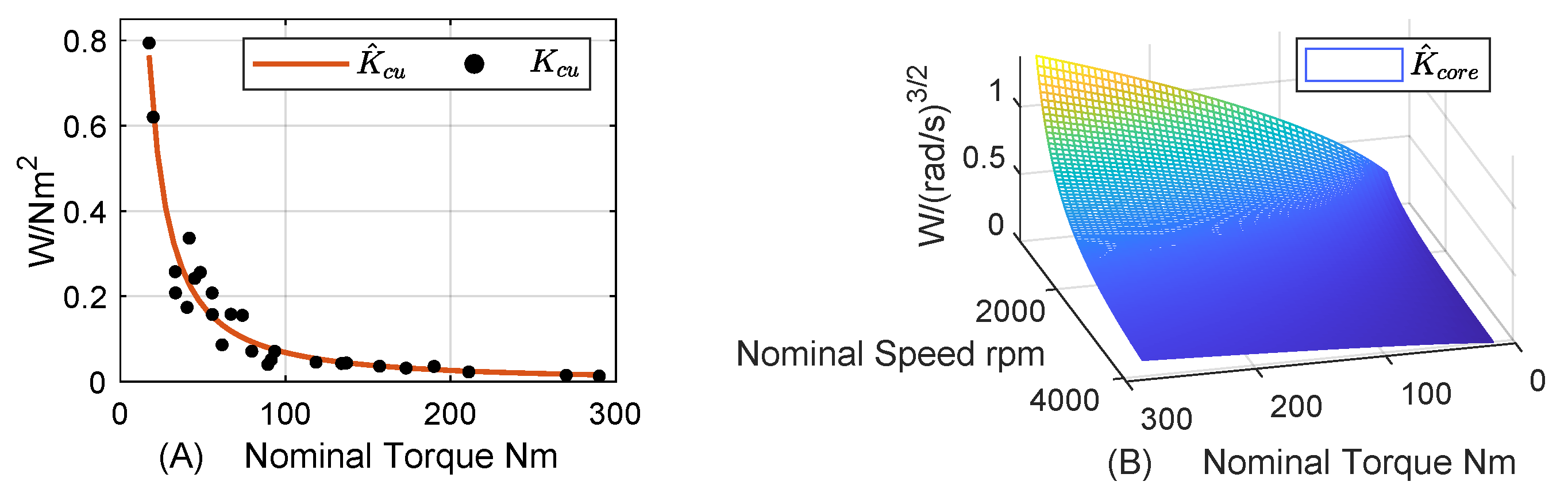
Considering the water cooled versions of the MS2N series, i.e., the water cooled versions of the MS2N07, MS2N10, and MS2N13, the trend of the copper loss coefficients $K_{\mathrm{cu}}$ as functions of nominal torque and speed, respectively, appear as the discrete points depicted in Figure 7A. In order to be able to choose motors of a desired size, and estimate the related losses appropriately, the $K_{\mathrm{cu}}$-coefficients are estimated by a function covering the nominal torque and speed ranges of the considered MS2N’s. By curve fitting, the $K_{\mathrm{cu}}$-trends, the estimate ${\widehat{K}}_{\mathrm{cu}}$, and subsequently the estimate ${\widehat{K}}_{\mathrm{core}}$ appear as Equation (4), with $a_{\mathrm{cu}}=39.85$, $b_{\mathrm{cu}}=-1.384$:

$$\begin{array}{c}\hfill {\widehat{K}}_{\mathrm{cu}}=a_{\mathrm{cu}}{\tau }_{\mathrm{L},\mathrm{nom}}^{b_{\mathrm{cu}}},{\widehat{K}}_{\mathrm{core}}=\frac{{\epsilon }_{\mathrm{c}}{\widehat{K}}_{\mathrm{cu}}{\tau }_{\mathrm{L},\mathrm{nom}}^2}{{\omega }_{\mathrm{m},\mathrm{nom}}^{3/2}}\end{array}$$

(4)

The estimates ${\widehat{K}}_{\mathrm{cu}}$, ${\widehat{K}}_{\mathrm{core}}$ are depicted in Figure 7, with ${\widehat{K}}_{\mathrm{cu}}$ showing good resemblance with the trend of the discrete $K_{\mathrm{cu}}$ points.

4.2.3. Total VsD Losses

Considering a VsD with $D=D_{\mathrm{ref}}=D_{\mathrm{A}4\mathrm{FM}}=27.75$ ccm with maximum speed and pressure of 4000 rpm and 400 bar, respectively (corresponding to a maximum torque of 177 Nm), the electric motor nominal torque and nominal speed chosen are ${\tau }_{\mathrm{L},\mathrm{nom}}=177$ Nm and $n_{\mathrm{m},\mathrm{nom}}=4000$ rpm. The corresponding total VsD efficiency and the efficiencies of the displacement unit, motor, and inverter are illustrated in Figure 8. Here, ${\eta }_{\mathrm{T}}$, ${\eta }_{\mathrm{D}}$, ${\eta }_{\mathrm{M}}$ and ${\eta }_{\mathrm{I}}$ correspond to the total, the displacement unit, the motor, and the inverter efficiencies, whereas ${\overline{\eta }}_{\mathrm{T}}$ and ${\eta }_{\mathrm{T},\max }$ correspond to the total mean and total maximum efficiencies.

4.3. Design of VDN with Point-to-Point Topology (VDN-PP)

Consider initially the well-known VDN with point-to-point topology (VDN-PP) depicted in Figure 9A. Indeed, from a cylinder point of view, these are hydraulically disconnected and only share the electric supply side.

For this topology, a VsD is interconnecting the chambers of each cylinder, while the VsD’s interconnecting each cylinder to tank can be connected to either the piston or rod side chambers.

4.3.1. Possible Displacement Unit Sizes for VDN-PP

The possible displacement unit sizes are investigated based on the specification in Section 4.1, with offset in the static flow continuities. Considering the example with the VDN-PP topology depicted in Figure 9B with 0 ↔ 1 and 0 ↔ 3, the pressure dynamics appear as Equations (5) and (6):

$$\begin{array}{cc}\hfill {\dot{p}}_1=\frac{\beta }{V_1}(Q_{1,0}+Q_{1,2}-A_1{\dot{x}}_1),& {\dot{p}}_2=\frac{\beta }{V_2}(A_2{\dot{x}}_1-Q_{1,2})\hfill \end{array}$$

(5)

$$\begin{array}{cc}\hfill {\dot{p}}_3=\frac{\beta }{V_3}(Q_{3,0}+Q_{3,4}-A_3{\dot{x}}_2),& {\dot{p}}_4=\frac{\beta }{V_4}(A_4{\dot{x}}_4-Q_{3,4})\hfill \\ \hfill Q_{1,0}=D_{1,0}{\omega }_{1,0},Q_{1,2}=D_{1,2}{\omega }_{1,2},& Q_{3,2}=D_{3,0}{\omega }_{3,0},Q_{3,4}=D_{3,4}{\omega }_{3,4}\hfill \end{array}$$

(6)

Applying the maximum speed specification from Section 4.1, $|{\omega }_{1,0,\max }|=|{\omega }_{1,2,\max }|=|{\omega }_{3,2,\max }|=|{\omega }_{3,4,\max }|=|{\omega }_{\max }|$ and maximum piston design velocities $|{\dot{x}}_{1,\max }|=|{\dot{x}}_{2,\max }|=|{\dot{x}}_{\max }|$, the necessary displacements under steady state conditions are expressed as Equations (7) and (8), bearing in mind that $A_1>A_2$, $A_3>A_4$, resulting in the displacement unit sizes in Equation (9):

$$\begin{array}{cc}\hfill D_{1,0}& =\pm \frac{(A_1-A_2)\left|{\dot{x}}_{max}\right|}{|{\omega }_{\max }|}\le \frac{(A_1-A_2)\left|{\dot{x}}_{max}\right|}{|{\omega }_{\max }|},D_{1,2}=\pm \frac{A_2\left|{\dot{x}}_{max}\right|}{|{\omega }_{\max }|}\le \frac{A_2\left|{\dot{x}}_{max}\right|}{|{\omega }_{\max }|}\hfill \end{array}$$

(7)

$$\begin{array}{cc}\hfill D_{3,0}& =\pm \frac{(A_3-A_4)\left|{\dot{x}}_{max}\right|}{|{\omega }_{\max }|}\le \frac{(A_3-A_4)\left|{\dot{x}}_{max}\right|}{|{\omega }_{\max }|},D_{3,4}=\pm \frac{A_4\left|{\dot{x}}_{max}\right|}{|{\omega }_{\max }|}\le \frac{A_4\left|{\dot{x}}_{max}\right|}{|{\omega }_{\max }|}\hfill \end{array}$$

(8)

$$\begin{array}{cc}\hfill \Rightarrow & D_{1,0}=32\left[ccm\right],D_{1,2}=31\left[ccm\right],D_{3,0}=26\left[ccm\right],D_{3,4}=24\left[ccm\right]\hfill \end{array}$$

(9)

Doing similar calculations for the tank interconnection schemes 0 ↔ 2, 0 ↔ 4 and 0 ↔ 1, 0 ↔ 4 and 0 ↔ 2, 0 ↔ 3, the necessary displacements appear as depicted in

Table 1. Necessary displacements in crane application for different interconnection schemes with VDN-PP topology. The blue colored case marks the scheme with the lowest displacement sum and the red colored case marks the scheme with the highest displacement sum.

Configuration	0 ↔ 1 & 0 ↔ 3	0 ↔ 2 & 0 ↔ 4	0 ↔ 1 & 0 ↔ 4	0 ↔ 2 & 0 ↔ 3
	[ccm]	[ccm]	[ccm]	[ccm]
1 ↔ 2 & 3 ↔ 4	32, 31, 26, 24	32, 62, 26, 50	32, 31, 26, 50	32, 62, 26, 24

. From this, the tank interconnection scheme 0 ↔ 1, 0 ↔ 3 appears as the more attractive one due to the lowest displacement unit sizes.

4.3.2. Possible Motor Sizes for VDN-PP

Considering the maximum torques for the different VDN-PP interconnection schemes as a result of the necessary displacements, the load, and the desired lower pressure level, these appear as depicted in

Table 2. Maximum shaft torques resulting from cylinder loads, lower pressure level, and necessary displacements for different interconnection schemes with VDN-PP topology. The Blue colored case marks the scheme with the lowest torque sum and the red colored case marks the scheme with the highest torque sum.

Configuration	0 ↔ 1 & 0 ↔ 3	0 ↔ 2 & 0 ↔ 4	0 ↔ 1 & 0 ↔ 4	0 ↔ 2 & 0 ↔ 3
	[Nm]	[Nm]	[Nm]	[Nm]
1 ↔ 2 & 3 ↔ 4	67, 56, 38, 57	10, 111, 70, 118	67, 56, 70, 118	10, 111, 38, 57

(see Appendix B for the pressure spectrum corresponding to the crane load). Evidently, the lowest maximum torques are achieved with the interconnection scheme 0 ↔ 1, 0 ↔ 3 and the largest maximum torques are achieved with the interconnection scheme 0 ↔ 2, 0 ↔ 4. Hence, the interconnection scheme with the lowest displacement is coincident with the one yielding the lowest displacement unit torque, and hence the lowest electric motor torque.

4.3.3. Choice of VDN-PP Interconnection Scheme

The VDN-PP with the tank interconnection scheme 0 ↔ 1, 0 ↔ 3 depicted in Figure 10 is found to be the more feasible one in relation to the crane application, as this is subject to both the lowest total displacement as well as the lowest shaft torques, i.e., with displacements $D_{1,0}=$ 32 [ccm], $D_{1,2}=$ 31 [ccm], $D_{3,0}=$ 26 [ccm], $D_{3,4}=$ 24 [ccm] and nominal motor torques ${\tau }_{1,0,\mathrm{nom}}$ = 67 [Nm], ${\tau }_{1,2,\mathrm{nom}}$ = 56 [Nm], ${\tau }_{3,0,\mathrm{nom}}$ = 38 [Nm], ${\tau }_{3,4,\mathrm{nom}}$ = 57 [Nm]. With the nominal shaft speeds equal to ${\omega }_{\max }$, the ideal nominal installed power is given by $P_{\mathrm{nom}}=({\tau }_{1,0,\mathrm{nom}}+{\tau }_{1,2,\mathrm{nom}}+{\tau }_{3,0,\mathrm{nom}}+{\tau }_{3,4,\mathrm{nom}}){\omega }_{\max }=$ 68.49 [kW].

The schematic of this VDN-PP is already depicted in Figure 9B, and when including the cross-port leakage and drain flows, its pressure dynamics may be described by Equations (11)–(13). Here, $Q_{\mathrm{L}1,0}=Q_{\mathrm{L}1,0}({\omega }_{1,0},p_1,p_0)$, $Q_{\mathrm{L}1,2}=Q_{\mathrm{L}1,2}({\omega }_{1,2},p_1,p_2)$, $Q_{\mathrm{L}3,0}=Q_{\mathrm{L}3,0}({\omega }_{3,0},p_3,p_0)$, $Q_{\mathrm{L}3,4}=Q_{\mathrm{L}3,4}({\omega }_{3,4},p_3,p_4)$ and $Q_{\mathrm{D}1,0|1}=Q_{\mathrm{D}1,0|1}({\omega }_{1,0},p_1,p_0)$, $Q_{\mathrm{D}1,2|1}=Q_{\mathrm{D}1,2|1}({\omega }_{1,2},p_1,p_0)$, $Q_{\mathrm{D}1,2|2}=Q_{\mathrm{D}1,2|2}({\omega }_{1,2},p_2,p_0)$, $Q_{\mathrm{D}3,0|3}=Q_{\mathrm{D}3,0|3}({\omega }_{3,0},p_3,p_0)$, $Q_{\mathrm{D}3,4|3}$$=Q_{\mathrm{D}3,4|3}({\omega }_{3,4},p_3,p_0)$, $Q_{\mathrm{D}3,4|4}=Q_{\mathrm{D}3,4|4}({\omega }_{3,4},p_4,p_0)$ are leakage and drain flows, respectively.

$$\begin{array}{cc}\hfill {\dot{p}}_1& =\frac{\beta }{V_1}(D_{1,0}{\omega }_{1,0}+D_{1,2}{\omega }_{1,2}-A_1{\dot{x}}_1-Q_{\mathrm{L}1,0}-Q_{\mathrm{L}1,2}-Q_{\mathrm{D}1,0|1}-Q_{\mathrm{D}1,2|1})\hfill \end{array}$$

(10)

$$\begin{array}{cc}\hfill {\dot{p}}_2& =\frac{\beta }{V_2}(A_2{\dot{x}}_1-D_{1,2}{\omega }_{1,2}+Q_{\mathrm{L}1,2}-Q_{\mathrm{D}1,2|2})\hfill \end{array}$$

(11)

$$\begin{array}{cc}\hfill {\dot{p}}_3& =\frac{\beta }{V_3}(D_{3,0}{\omega }_{3,0}+D_{3,4}{\omega }_{3,4}-A_3{\dot{x}}_2-Q_{\mathrm{L}3,0}-Q_{\mathrm{L}3,4}-Q_{\mathrm{D}3,0|3}-Q_{\mathrm{D}3,4|3})\hfill \end{array}$$

(12)

$$\begin{array}{cc}\hfill {\dot{p}}_4& =\frac{\beta }{V_4}(A_4{\dot{x}}_4-D_{3,4}{\omega }_{3,4}+Q_{\mathrm{L}3,4}-Q_{\mathrm{D}3,4|4})\hfill \end{array}$$

(13)

4.4. Design of VDN with Linear Topology (VDN-L)

Consider the linear VDN topology depicted in Figure 11A. In this example, VsD’s are interconnecting chambers 1 ↔ 2, 2 ↔ 3 and 3 ↔ 4; however, several interconnection schemes exist.

The possible chamber interconnections, disregarding the tank interconnecting VsD, are shown in

Table 3. Possible chamber interconnection schemes of VDN with linear topology in dual cylinder crane application. Blue colored combinations represent redundant interconnection schemes.

1↔2↔3↔4	1↔3↔2↔4	1↔2↔4↔3	1↔4↔3↔2	1↔3↔4↔2	1↔4↔2↔3
2↔1↔3↔4	2↔3↔1↔4	2↔1↔4↔3	2↔4↔1↔3	2↔3↔4↔1	2↔4↔3↔1
3↔1↔2↔4	3↔2↔1↔4	3↔1↔4↔2	3↔4↔1↔2	3↔2↔4↔1	3↔4↔2↔1
4↔1↔2↔3	4↔2↔1↔3	4↔1↔3↔2	4↔3↔1↔2	4↔2↔3↔1	4↔3↔2↔1

where the first entry corresponds to the interconnection scheme depicted in Figure 11A. In total, 24 possible interconnection schemes exist, of which half are redundant as e.g., 1 ↔ 2 ↔ 3 ↔ 4 equals 4 ↔ 3 ↔ 2 ↔ 1, and so forth. Hence, 12 unique chamber interconnection schemes exist. In addition, the reservoir may be interconnected to either of the four cylinder chambers for each of the 12 chamber interconnection schemes, amounting to a total of 48 unique interconnection schemes for a dual actuator VDN with linear topology.

4.4.1. Possible Displacement Unit Sizes for VDN-L

Consider the schematics of Figure 11B with chamber 1 connected to 0, i.e., the interconnection scheme 1 ↔ 2 ↔ 3 ↔ 4, 0 ↔ 1. Assuming ideal components, the pressure dynamics of this VDN-L may be modeled by Equations (14)–(16):

$$\begin{array}{cc}\hfill {\dot{p}}_1=\frac{\beta }{V_1}(Q_{1,0}+Q_{1,2}-A_1{\dot{x}}_1),& {\dot{p}}_2=\frac{\beta }{V_2}(A_2{\dot{x}}_1-Q_{1,2}-Q_{3,2})\hfill \end{array}$$

(14)

$$\begin{array}{cc}\hfill {\dot{p}}_3=\frac{\beta }{V_3}(Q_{3,2}+Q_{3,4}-A_3{\dot{x}}_2),& {\dot{p}}_4=\frac{\beta }{V_4}(A_4{\dot{x}}_4-Q_{3,4})\hfill \end{array}$$

(15)

$$\begin{array}{cc}\hfill Q_{1,0}=D_{1,0}{\omega }_{1,0},Q_{1,2}=D_{1,2}{\omega }_{1,2},& Q_{3,2}=D_{3,2}{\omega }_{3,2},Q_{3,4}=D_{3,4}{\omega }_{3,4}\hfill \end{array}$$

(16)

Still applying the design requirement of maximum shaft speeds of $|{\omega }_{1,0,\max }|=|{\omega }_{1,2,\max }|=|{\omega }_{3,2,\max }|=|{\omega }_{3,4,\max }|=|{\omega }_{\max }|$ and maximum piston velocities $|{\dot{x}}_{1,\max }|=|{\dot{x}}_{2,\max }|=|{\dot{x}}_{\max }|$, the ideal displacement sizes may be found from Equations (14)–(16) under steady state conditions as Equations (17)–(20), noting that $A_1>A_2$, $A_3>A_4$.

$$\begin{array}{cc}\hfill D_{1,0}& =\pm \frac{(A_1-A_2)\left|{\dot{x}}_{\max }\right|}{|{\omega }_{\max }|}\pm \frac{(A_3-A_4)\left|{\dot{x}}_{\max }\right|}{|{\omega }_{\max }|}\le \frac{(A_1-A_2)\left|{\dot{x}}_{\max }\right|}{|{\omega }_{\max }|}+\frac{(A_3-A_4)\left|{\dot{x}}_{\max }\right|}{|{\omega }_{\max }|}\hfill \end{array}$$

(17)

$$\begin{array}{cc}\hfill D_{1,2}& =\pm \frac{A_2\left|{\dot{x}}_{\max }\right|}{|{\omega }_{\max }|}\pm \frac{(A_4-A_3)\left|{\dot{x}}_{\max }\right|}{|{\omega }_{\max }|}\le \frac{A_2\left|{\dot{x}}_{\max }\right|}{|{\omega }_{\max }|}+\frac{(A_4-A_3)\left|{\dot{x}}_{\max }\right|}{|{\omega }_{\max }|}\hfill \end{array}$$

(18)

$$\begin{array}{cc}\hfill D_{3,2}& =\pm \frac{(A_3-A_4)\left|{\dot{x}}_{\max }\right|}{|{\omega }_{\max }|}\le \frac{(A_3-A_4)\left|{\dot{x}}_{\max }\right|}{|{\omega }_{\max }|}\hfill \end{array}$$

(19)

$$\begin{array}{cc}\hfill D_{3,4}& =\mp \frac{A_4\left|{\dot{x}}_{\max }\right|}{|{\omega }_{\max }|}\le \frac{A_4\left|{\dot{x}}_{\max }\right|}{|{\omega }_{\max }|}\hfill \end{array}$$

(20)

By evaluation, the displacement sizes necessary to realize the desired motion functionality are given by Equaiton (21):

$$\begin{array}{c}\hfill D_{1,0}=57\left[ccm\right],D_{1,2}=56\left[ccm\right],D_{3,2}=26\left[ccm\right],D_{3,4}=24\left[ccm\right]\end{array}$$

(21)

Doing similar calculations for all 48 unique interconnection schemes, the corresponding necessary displacements appear as given in

Table 4. Necessary displacements for linear VDN topology interconnection schemes in crane application. The Blue colored case marks the scheme with the lowest displacement sum and the red colored cases mark the scheme with the highest displacement sum.

Configuration	0 ↔ 1	0 ↔ 2	0 ↔ 3	0 ↔ 4
	[ccm]	[ccm]	[ccm]	[ccm]
1 ↔ 2 ↔ 3 ↔ 4	58, 57, 26, 24	58, 62, 26, 24	58, 62, 32, 24	57, 62, 32, 81
1 ↔ 3 ↔ 2 ↔ 4	58, 54, 57, 24	58, 112, 62, 24	58, 54, 62, 24	57, 111, 62, 81
1 ↔ 2 ↔ 4 ↔ 3	58, 57, 26, 50	58, 62, 26, 50	58, 62, 32, 57	57, 62, 32, 50
1 ↔ 4 ↔ 3 ↔ 2	58, 31, 57, 80	58, 88, 62, 86	58, 31, 62, 86	57, 31, 62, 80
1 ↔ 3 ↔ 4 ↔ 2	58, 31, 57, 54	58, 88, 62, 112	58, 31, 62, 54	57, 31, 62, 111
1 ↔ 4 ↔ 2 ↔ 3	58, 80, 50, 57	58, 86, 50, 62	58, 86, 57, 62	57, 80, 50, 62
2 ↔ 1 ↔ 3 ↔ 4	58, 31, 26, 24	58, 88, 26, 24	58, 31, 32, 24	57, 31, 32, 81
2 ↔ 3 ↔ 1 ↔ 4	58, 31, 80, 24	58, 88, 86, 24	58, 31, 86, 24	57, 31, 80, 81
2 ↔ 1 ↔ 4 ↔ 3	58, 31, 26, 50	58, 88, 26, 50	58, 31, 32, 57	57, 31, 32, 50
2 ↔ 4 ↔ 1 ↔ 3	58, 50, 54, 31	58, 50, 112, 88	58, 57, 54, 31	57, 50, 111, 31
3 ↔ 1 ↔ 2 ↔ 4	58, 54, 50, 24	58, 112, 50, 24	58, 54, 57, 24	57, 111, 50, 81
3 ↔ 2 ↔ 1 ↔ 4	58, 50, 80, 24	58, 50, 86, 24	58, 57, 86, 24	57, 50, 80, 81

. Evidently, the necessary displacements vary significantly across the 48 interconnection schemes with a least total displacement of 139 [ccm] for the scheme 2 ↔ 1 ↔ 3 ↔ 4, 0 ↔ 1 (blue font) and a maximum total displacement of 320 [ccm] for the scheme 1 ↔ 3 ↔ 4 ↔ 2, 0 ↔ 2 (red font).

4.4.2. Possible Motor Sizes for VDN-L

The pressure differences are dictated by the load and the desired minimum pressure level as illustrated in Appendix B. Therefore, the different displacements give rise to very different displacement unit torques, hence the required electric motor sizes. The maximum shaft torques resulting from the load, desired pressure level and the necessary displacements are tabulated in

Table 5. Maximum shaft torques for linear VDN topology interconnection schemes in crane application. The Blue colored case marks the scheme with the lowest torque sum and the red colored cases mark the schemes with the highest torque sum.

Configuration	0 ↔ 1	0 ↔ 2	0 ↔ 3	0 ↔ 4
	[Nm]	[Nm]	[Nm]	[Nm]
1 ↔ 2 ↔ 3 ↔ 4	120, 100, 30, 57	18, 111, 30, 57	84, 111, 37, 57	152, 111, 37, 191
1 ↔ 3 ↔ 2 ↔ 4	120, 62, 82, 57	18, 128, 91, 57	84, 62, 91, 57	152, 128, 91, 191
1 ↔ 2 ↔ 4 ↔ 3	120, 100, 61, 118	18, 111, 61, 118	84, 111, 75, 132	152, 111, 75, 118
1 ↔ 4 ↔ 3 ↔ 2	120, 36, 100, 188	18, 102, 111, 203	84, 36, 111, 203	152, 36, 111, 188
1 ↔ 3 ↔ 4 ↔ 2	120, 73, 82, 127	18, 207, 91, 261	84, 73, 91, 127	152, 73, 91, 261
1 ↔ 4 ↔ 2 ↔ 3	120, 188, 58, 100	18, 203, 58, 111	84, 203, 65, 111	152, 188, 58, 111
2 ↔ 1 ↔ 3 ↔ 4	120, 56, 38, 57	18, 158, 38, 57	84, 56, 47, 57	152, 56, 47, 191
2 ↔ 3 ↔ 1 ↔ 4	120, 36, 118, 43	18, 102, 127, 43	84, 36, 127, 43	152, 36, 118, 145
2 ↔ 1 ↔ 4 ↔ 3	120, 56, 47, 118	18, 158, 47, 118	84, 56, 57, 132	152, 56, 57, 118
2 ↔ 4 ↔ 1 ↔ 3	120, 74, 97, 73	18, 74, 199, 207	84, 82, 97, 73	152, 74, 199, 73
3 ↔ 1 ↔ 2 ↔ 4	120, 97, 74, 57	18, 199, 74, 57	84, 97, 82, 57	152, 199, 74, 191
3 ↔ 2 ↔ 1 ↔ 4	120, 58, 143, 43	18, 58, 154, 43	84, 65, 154, 43	152, 58, 143, 145

. The interconnection scheme subject to the lowest maximum torque sum is the scheme 2 ↔ 1 ↔ 3 ↔ 4, 0 ↔ 3 (blue font), which is not the one with the lowest necessary displacements. The interconnection schemes having the largest maximum torque sums are the schemes 1 ↔ 3 ↔ 4 ↔ 2, 0 ↔ 2 and 1 ↔ 3 ↔ 4 ↔ 2, 0 ↔ 4 (both with red font), with different distributions between the four VsD’s. Hence, for the crane application, the VDN-L scheme with the lowest displacement does not yield the lowest individual displacement unit torques and hence required motor sizes.

4.4.3. Choice of the VDN-L Interconnection Scheme

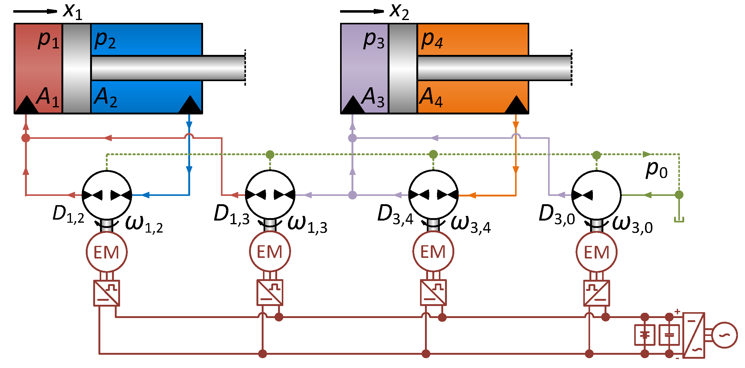
From the above, the most feasible VDN-L interconnection scheme for the crane application is the one characterized by the interconnections 2 ↔ 1 ↔ 3 ↔ 4, 0 ↔ 3, viewed in the context of component sizes and the assumption that the electric motor and associated inverter in general are the more cost intensive VsD components. Hence, this scheme is chosen for further consideration, with the schematics depicted in Figure 12.

The displacement sizes are $D_{3,0}$ = 58 [ccm], $D_{1,2}$ = 31 [ccm], $D_{1,3}$ = 32 [ccm], $D_{3,4}$ = 24 [ccm], and the nominal motor torques ${\tau }_{3,0,\mathrm{nom}}$ = 84 [Nm], ${\tau }_{1,2,\mathrm{nom}}$ = 56 [Nm], ${\tau }_{1,3,\mathrm{nom}}$ = 47 [Nm], ${\tau }_{3,4,\mathrm{nom}}$ = 57 [Nm]. With the nominal shaft speeds equal to ${\omega }_{\max }$, the nominal installed power then amounts to $P_{\mathrm{nom}}=({\tau }_{1,3,\mathrm{nom}}+{\tau }_{1,2,\mathrm{nom}}+{\tau }_{3,0,\mathrm{nom}}+{\tau }_{3,4,\mathrm{nom}}){\omega }_{\max }=$ 76.65 [kW].

The describing equations for the pressure dynamics are given by Equations (22)–(25), where $Q_{\mathrm{L}3,0}=Q_{\mathrm{L}3,0}({\omega }_{3,0},p_3,p_0)$, $Q_{\mathrm{L}1,2}=Q_{\mathrm{L}1,2}({\omega }_{1,2},p_1,p_2)$, $Q_{\mathrm{L}1,3}=Q_{\mathrm{L}1,3}({\omega }_{1,3},p_1,p_3)$ and $Q_{\mathrm{L}3,4}=Q_{\mathrm{L}3,4}({\omega }_{3,4},p_3,p_4)$ are the displacement unit cross-port leakage flows and $Q_{\mathrm{D}3,0|3}=Q_{\mathrm{D}3,0|3}({\omega }_{3,0},p_3,p_0)$, $Q_{\mathrm{D}1,2|1}=Q_{\mathrm{D}1,2|1}({\omega }_{1,2},p_1,p_0)$, $Q_{\mathrm{D}1,2|2}$$=Q_{\mathrm{D}1,2|2}({\omega }_{1,2},p_2,p_0)$, $Q_{\mathrm{D}1,3|1}=Q_{\mathrm{D}1,3|1}({\omega }_{1,3},p_1,p_0)$, $Q_{\mathrm{D}1,3|3}=Q_{\mathrm{D}1,3|3}({\omega }_{1,3},p_3,p_0)$, $Q_{\mathrm{D}3,4|3}=Q_{\mathrm{D}3,4|3}({\omega }_{3,4},p_3,p_0)$, $Q_{\mathrm{D}3,4|4}=Q_{\mathrm{D}3,4|4}({\omega }_{3,4},p_4,p_0)$ are the displacement unit drain flows.

$$\begin{array}{cc}\hfill {\dot{p}}_1& =\frac{\beta }{V_1}(D_{1,3}{\omega }_{1,3}+D_{1,2}{\omega }_{1,2}-A_1{\dot{x}}_1-Q_{\mathrm{L}1,2}-Q_{\mathrm{L}1,3}-Q_{\mathrm{D}1,2|1}-Q_{\mathrm{D}1,3|1})\hfill \end{array}$$

(22)

$$\begin{array}{cc}\hfill {\dot{p}}_2& =\frac{\beta }{V_2}(A_2{\dot{x}}_1-D_{1,2}{\omega }_{1,2}+Q_{\mathrm{L}1,2}-Q_{\mathrm{D}1,2|2})\hfill \end{array}$$

(23)

$$\begin{array}{cc}\hfill {\dot{p}}_3& =\frac{\beta }{V_3}(D_{3,0}{\omega }_{3,0}-D_{1,3}{\omega }_{1,3}+D_{3,4}{\omega }_{3,4}-A_3{\dot{x}}_2-Q_{\mathrm{L}3,0}+Q_{\mathrm{L}1,3}-Q_{\mathrm{L}3,4}\hfill \\ \hfill & -Q_{\mathrm{D}3,0|3}-Q_{\mathrm{D}1,3|3}-Q_{\mathrm{D}3,4|3})\hfill \end{array}$$

(24)

$$\begin{array}{cc}\hfill {\dot{p}}_4& =\frac{\beta }{V_4}(A_4{\dot{x}}_2-D_{3,4}{\omega }_{3,4}+Q_{\mathrm{L}3,4}-Q_{\mathrm{D}3,4|4})\hfill \end{array}$$

(25)

4.5. Design of VDN with Linear Topology and Shared Chambers (VDN-LS)

The possibility for sharing chambers will allow for reducing the number of components compared to the VDN-PP and VDN-L. If feasible, this may in addition reduce conversion losses and simplify component integration on a systems level, all features of commercial relevance.

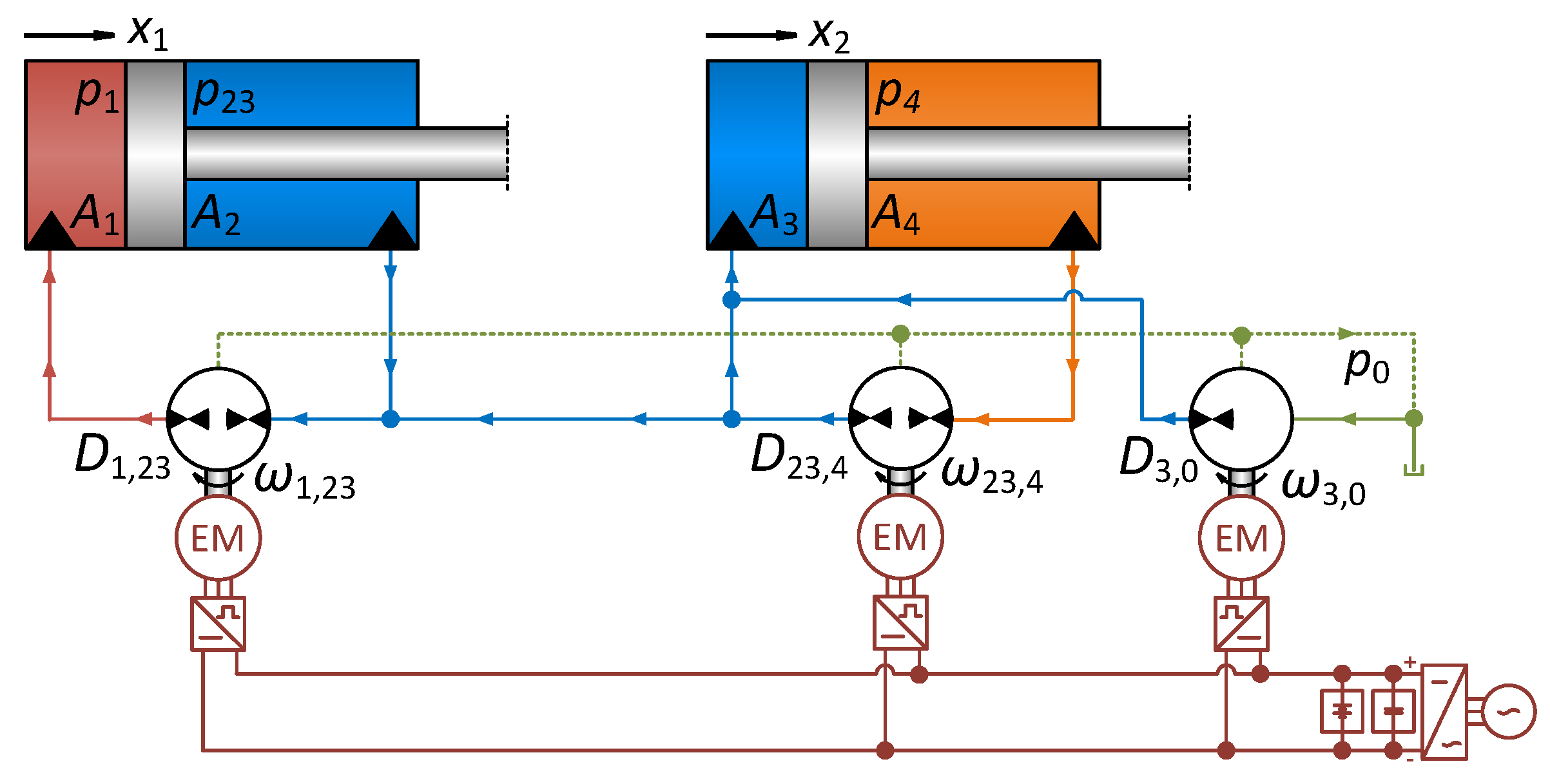
Consider the linear VDN topology with shared chambers (VDN-LS) depicted in Figure 13A. This is similar to the VDN-L depicted in Figure 11A, with the difference that the VsD interconnecting chambers 2 and 3 have been omitted, directly short circuiting these.

Considering each chamber and its possible interconnections to the other chambers, 24 possible interconnection schemes also exist here due to the different possibilities of sharing chambers. Again, half of these are redundant as illustrated in

Table 6. Possible chamber interconnection schemes of VDN with linear topology and shared chambers in dual cylinder crane application. Blue colored combinations represent redundant interconnection schemes.

13↔2↔4	13↔4↔2	2↔13↔4	1↔23↔4	23↔4↔1	23↔1↔4
14↔2↔3	14↔3↔2	2↔14↔3	24↔1↔3	24↔3↔1	1↔24↔3
4↔2↔13	2↔4↔13	4↔13↔2	4↔23↔1	1↔4↔23	4↔1↔23
3↔2↔14	2↔3↔14	3↔14↔2	3↔1↔24	1↔3↔24	3↔24↔1

. In addition, each of the three resulting chambers may be interconnected to the tank, yielding 36 unique VDN-LS interconnection schemes.

4.5.1. Possible Displacement Unit Sizes for VDN-LS

Considering the interconnection scheme illustrated in Figure 13B, the pressure dynamics may be modeled as Equations (26) and (27):

$$\begin{array}{cc}\hfill {\dot{p}}_1& =\frac{\beta }{V_1}(Q_{1,0}+Q_{1,23}-A_1{\dot{x}}_1),{\dot{p}}_{23}=\frac{\beta }{V_{23}}(Q_{23,4}-Q_{1,23}+A_2{\dot{x}}_1-A_3{\dot{x}}_2)\hfill \end{array}$$

(26)

$$\begin{array}{cc}\hfill {\dot{p}}_4& =\frac{\beta }{V_4}(A_4{\dot{x}}_4-Q_{23,4}),Q_{1,0}=D_{1,0}{\omega }_{1,0},Q_{1,23}=D_{1,23}{\omega }_{1,23},Q_{23,4}=D_{23,4}{\omega }_{23,4}\hfill \end{array}$$

(27)

Again, applying the design specifications, i.e., $|{\omega }_{1,0,\max }|=|{\omega }_{23,4,\max }|=|{\omega }_{1,23,\max }|=|{\omega }_{\max }|$ and $|{\dot{x}}_{1,max}|=|{\dot{x}}_{2,max}|=|{\dot{x}}_{max}|$, the necessary displacements may be found as Equation (31) under steady state conditions.

$$\begin{array}{cc}\hfill D_{1,0}& =\pm \frac{(A_1-A_2)\left|{\dot{x}}_{\max }\right|}{|{\omega }_{\max }|}\pm \frac{(A_3-A_4)\left|{\dot{x}}_{\max }\right|}{|{\omega }_{\max }|}\hfill \\ \hfill & \le \frac{(A_1-A_2)\left|{\dot{x}}_{\max }\right|}{|{\omega }_{\max }|}+\frac{(A_3-A_4)\left|{\dot{x}}_{\max }\right|}{|{\omega }_{\max }|}\hfill \end{array}$$

(28)

$$\begin{array}{cc}\hfill D_{1,23}& =\mp \frac{(A_4-A_3)\left|{\dot{x}}_{\max }\right|}{|{\omega }_{\max }|}\pm \frac{A_2\left|{\dot{x}}_{\max }\right|}{|{\omega }_{\max }|}\le \frac{(A_4-A_3)\left|{\dot{x}}_{\max }\right|}{|{\omega }_{\max }|}+\frac{A_2\left|{\dot{x}}_{\max }\right|}{|{\omega }_{\max }|}\hfill \end{array}$$

(29)

$$\begin{array}{cc}\hfill D_{23,4}& =\pm \frac{A_4\left|{\dot{x}}_{\max }\right|}{|{\omega }_{\max }|}\le \frac{A_4\left|{\dot{x}}_{\max }\right|}{|{\omega }_{\max }|}\hfill \end{array}$$

(30)

$$\begin{array}{cc}\hfill & \Rightarrow D_{1,0}=58\left[ccm\right],D_{1,23}=57\left[ccm\right],D_{23,4}=24\left[ccm\right]\hfill \end{array}$$

(31)

Doing similar calculations for all 36 unique interconnection schemes, their necessary displacements appear as in

Table 7. Necessary displacements for linear VDN topology interconnection schemes with shared chambers in crane application. The Blue colored cases mark the schemes with displacement sums below 150 [ccm] and the red colored case marks the scheme with the highest displacement sum.

Configuration	0 ↔ 13	0 ↔ 2	0 ↔ 4
13 ↔ 2 ↔ 4	54, 58, 24 [ccm]	112, 58, 24 [ccm]	112, 58, 81 [ccm]
13 ↔ 4 ↔ 2	54, 58, 31 [ccm]	112, 58, 88 [ccm]	112, 58, 31 [ccm]
2 ↔ 13↔ 4	31, 58, 24 [ccm]	88, 58, 24 [ccm]	31, 58, 81 [ccm]
Configuration	0 ↔ 14	0 ↔ 2	0 ↔ 3
14 ↔ 2 ↔ 3	80, 58, 50 [ccm]	86, 58, 50 [ccm]	86, 58, 57 [ccm]
14 ↔ 3 ↔ 2	80, 58, 31 [ccm]	86, 58, 88 [ccm]	86, 58, 31 [ccm]
2 ↔ 14 ↔ 3	31, 58, 50 [ccm]	88, 58, 50 [ccm]	31, 58, 57 [ccm]
Configuration	0 ↔ 23	0 ↔ 1	0 ↔ 4
23 ↔ 1 ↔ 4	86, 58, 24 [ccm]	80, 58, 24 [ccm]	80, 58, 81 [ccm]
23 ↔ 4 ↔ 1	86, 58, 62 [ccm]	80, 58, 57 [ccm]	80, 58, 62 [ccm]
1 ↔ 23 ↔ 4	62, 58, 24 [ccm]	57, 58, 24 [ccm]	62, 58, 81 [ccm]
Configuration	0 ↔ 24	0 ↔ 1	0 ↔ 3
24 ↔ 1 ↔ 3	112, 58, 50 [ccm]	54, 58, 50 [ccm]	54, 58, 57 [ccm]
24 ↔ 3 ↔ 1	112, 58, 62 [ccm]	54, 58, 57 [ccm]	54, 58, 62 [ccm]
1 ↔ 24 ↔ 3	62, 58, 50 [ccm]	57, 58, 50 [ccm]	62, 58, 57 [ccm]

. By inspection, especially the six schemes marked by blue font differ from the remaining by exhibiting rather low displacements, with their total necessary displacements below 150 [ccm]. For the scheme 2 ↔ 13 ↔ 4 with 0 ↔ 13, the total displacement amounts to 113 [ccm], and for the scheme 13 ↔ 4 ↔ 2 with 0 ↔ 2, the total displacement is 258 [ccm].

4.5.2. Possible Motor Sizes for VDN-LS

The maximum torques corresponding to the necessary displacements, the load and lower pressure setting are shown in

Table 8. Maximum shaft torques for linear VDN topology interconnection schemes with shared chambers in crane application. The Blue colored case marks the scheme with lowest torque sum and the red colored case marks the scheme with the highest torque sum.

Configuration	0 ↔ 13	0 ↔ 2	0 ↔ 4
13 ↔ 2 ↔ 4	97, 120, 94 [Nm]	199, 18, 94 [Nm]	199, 243, 319 [Nm]
13 ↔ 4 ↔ 2	170, 120, 122 [Nm]	350, 18, 122 [Nm]	350, 243, 122 [Nm]
2 ↔ 13 ↔ 4	56, 120, 76 [Nm]	158, 18, 76 [Nm]	56, 243, 255 [Nm]
Configuration	0 ↔ 14	0 ↔ 2	0 ↔ 3
14 ↔ 2 ↔ 3	143, 152, 165 [Nm]	154, 206, 165 [Nm]	154, 133, 185 [Nm]
14 ↔ 3 ↔ 2	188, 152, 102 [Nm]	203, 206, 290 [Nm]	203, 133, 102 [Nm]
2 ↔ 14 ↔ 3	56, 152, 118 [Nm]	158, 206, 118 [Nm]	56, 133, 132 [Nm]
Configuration	0 ↔ 23	0 ↔ 1	0 ↔ 4
23 ↔ 1 ↔ 4	127, 84, 57 [Nm]	118, 152, 57 [Nm]	118, 152, 191 [Nm]
23 ↔ 4 ↔ 1	203, 84,146 [Nm]	188, 152, 132 [Nm]	188, 152, 146 [Nm]
1 ↔ 23 ↔ 4	91, 84, 57 [Nm]	82, 152, 57 [Nm]	91, 152, 191 [Nm]
Configuration	0 ↔ 24	0 ↔ 1	0 ↔ 3
24 ↔ 1 ↔ 3	199, 152, 96 [Nm]	97, 127, 96 [Nm]	97, 84, 107 [Nm]
24 ↔ 3 ↔ 1	261, 152, 119 [Nm]	127, 127, 107 [Nm]	127, 84, 119 [Nm]
1 ↔ 24 ↔ 3	111, 152, 118 [Nm]	100, 127, 118 [Nm]	111, 84, 132 [Nm]

(see Appendix C for the different pressure spectra corresponding to the crane load). It is found that the maximum torque sum is lowest for the scheme 1 ↔ 23 ↔ 4, 0 ↔ 23, whereas the highest torque sum is found for the scheme 13 ↔ 4 ↔ 2, 0 ↔ 4.

The reason for the rather high maximum torque in some cases is a consequence of the pressures resulting from infeasible chamber sharing.

4.5.3. Choice of VDN-LS Interconnection Scheme

With the main design objective being the VDN-LS scheme with the lowest possible motor torques, the VDN-LS interconnection scheme 1 ↔ 24 ↔ 4, 0 ↔ 23 is chosen for further consideration, with the schematics shown in Figure 14. For this scheme, the displacement sizes are $D_{23,0}$ = 58 [ccm], $D_{1,23}$ = 62 [ccm], $D_{23,4}$ = 24 [ccm] and the nominal shaft torques ${\tau }_{23,0,\mathrm{nom}}$ = 84 [Nm], ${\tau }_{1,23,\mathrm{nom}}$ = 91 [Nm], ${\tau }_{23,4,\mathrm{nom}}$ = 57 [Nm]. The ideal nominal power to be installed is given by $P_{\mathrm{nom}}=({\tau }_{1,23,\mathrm{nom}}+{\tau }_{23,0,\mathrm{nom}}+{\tau }_{23,4,\mathrm{nom}}){\omega }_{\max }=$ 72.88 [kW].

The corresponding VDN-LS pressure dynamics may be described by Equations (32)– (34) where $Q_{\mathrm{L}23,0}=Q_{\mathrm{L}23,0}({\omega }_{23,0},p_{23},p_0)$, $Q_{\mathrm{L}1,23}=Q_{\mathrm{L}1,23}({\omega }_{1,23},p_1,p_{2}3)$, $Q_{\mathrm{L}23,4}=$$Q_{\mathrm{L}23,4}({\omega }_{23,4},p_{23},p_4)$ are cross port leakage flows and $Q_{\mathrm{D}23,0|23}=Q_{\mathrm{D}23,0|23}({\omega }_{23,0},p_{23},p_0)$, $Q_{\mathrm{D}1,23|1}=Q_{\mathrm{D}1,23|1}({\omega }_{1,23},p_1,p_0)$, $Q_{\mathrm{D}1,23|23}=Q_{\mathrm{D}1,23|23}({\omega }_{1,23},p_{23},p_0)$, $Q_{\mathrm{D}23,4|23}=$$Q_{\mathrm{D}23,4|23}({\omega }_{23,4},p_{2}3,p_0)$, $Q_{\mathrm{D}23,4|4}=Q_{\mathrm{D}23,4|4}({\omega }_{23,4},p_4,p_0)$ are displacement unit drain flows:

$$\begin{array}{cc}\hfill {\dot{p}}_1& =\frac{\beta }{V_1}(D_{1,23}{\omega }_{1,23}-A_1{\dot{x}}_1-Q_{\mathrm{L}1,23}-Q_{\mathrm{D}1,23|1})\hfill \end{array}$$

(32)

$$\begin{array}{cc}\hfill {\dot{p}}_{23}& =\frac{\beta }{V_{23}}(A_2{\dot{x}}_1-A_3{\dot{x}}_2+D_{23,0}{\omega }_{23,0}-D_{1,23}{\omega }_{1,23}+D_{23,4}{\omega }_{23,4}-Q_{\mathrm{L}23,0}+Q_{\mathrm{L}1,23}\hfill \\ \hfill & -Q_{\mathrm{L}23,4}-Q_{\mathrm{D}23,0|23}-Q_{\mathrm{D}1,23|23}-Q_{\mathrm{D}23,4|23})\hfill \end{array}$$

(33)

$$\begin{array}{cc}\hfill {\dot{p}}_4& =\frac{\beta }{V_4}(A_4{\dot{x}}_2-D_{23,4}{\omega }_{23,4}+Q_{\mathrm{L}23,4}-Q_{\mathrm{D}23,4|4})\hfill \end{array}$$

(34)

4.6. Control Design for Chosen VDN Topologies

All three VDN topologies chosen for further consideration are subject to coupled dynamics, however with different intensity. Hence, control of, e.g., the individual cylinder motions may appear complicated to establish; however, physically motivated nonlinear flow decoupling schemes may be rather easily realized based on the flow continuity equations, as will be clear from the following. Flow decoupling schemes for each of the chosen VDN’s will be derived including load and sum pressure controllers. The control variables of the compensating structures are the load and sum pressures, and take the corresponding references as inputs, hence forming a cascade control structure when closing the motion control loops. The system control structure is exemplified in Figure 15 for the VDN-PP, and is similar for the VDN-L and VDN-LS. Note furthermore that the following assumes that only position and pressure measurements are available as feedback.

4.6.1. VDN-PP Flow Decoupling Scheme

The flow decoupling scheme for the VDN-PP can be derived for the individual axes as they are hydraulically separated. The load and sum pressure dynamics may be found from Equations (10)–(13) as Equations (35)–(38), when neglecting cross port leakage and drain flows:

$$\begin{array}{cc}\hfill {\dot{p}}_{\mathrm{L}1}& ={\dot{p}}_1-\frac{A_2}{A_1}{\dot{p}}_2=\frac{\beta }{V_1{V}_2{A}_1}(A_1{V}_2{D}_{1,0}{\omega }_{1,0}+(A_1{V}_2+A_2{V}_1)D_{1,2}{\omega }_{1,2}\hfill \\ \hfill & -(A_1^2{V}_2+A_2^2{V}_1){\dot{x}}_1)\hfill \end{array}$$

(35)

$$\begin{array}{cc}\hfill {\dot{p}}_{\Sigma 1}& ={\dot{p}}_1+{\dot{p}}_2=\frac{\beta }{V_1{V}_2}(V_2{D}_{1,0}{\omega }_{1,0}-(V_1-V_2)D_{1,2}{\omega }_{1,2}-(A_1{V}_2-A_2{V}_1){\dot{x}}_1)\hfill \end{array}$$

(36)

$$\begin{array}{cc}\hfill {\dot{p}}_{\mathrm{L}2}& ={\dot{p}}_3-\frac{A_4}{A_3}{\dot{p}}_4=\frac{\beta }{V_3{V}_4{A}_3}(A_3{V}_4{D}_{3,0}{\omega }_{3,0}+(A_3{V}_4+A_4{V}_3)D_{3,4}{\omega }_{3,4}\hfill \\ \hfill & -(A_3^4{V}_4+A_4^4{V}_3){\dot{x}}_2)\hfill \end{array}$$

(37)

$$\begin{array}{cc}\hfill {\dot{p}}_{\Sigma 2}& ={\dot{p}}_3+{\dot{p}}_4=\frac{\beta }{V_3{V}_4}(V_4{D}_{3,0}{\omega }_{3,0}-(V_3-V_4)D_{3,4}{\omega }_{3,4}-(A_3{V}_4-A_4{V}_3){\dot{x}}_2)\hfill \end{array}$$

(38)

For the load and sum pressure dynamics, all parameters are generally obtainable except from the bulk moduli. Furthermore, the piston velocities are assumed not available as mentioned above. The flow decoupling scheme is motivated by the idea of enforcing some desired or reference load and sum pressure dynamics given by Equations (39) and(40):

$$\begin{array}{cc}\hfill & {\dot{p}}_{\mathrm{L}1}^{\ast }={\omega }_{\mathrm{L}1}(p_{\mathrm{L}1}^{\ast }-p_{\mathrm{L}1}),{\dot{p}}_{\Sigma 1}^{\ast }={\omega }_{\Sigma 1}(p_{\Sigma 1}^{\ast }-p_{\Sigma 1})\hfill \end{array}$$

(39)

$$\begin{array}{cc}\hfill & {\dot{p}}_{\mathrm{L}2}^{\ast }={\omega }_{\mathrm{L}2}(p_{\mathrm{L}2}^{\ast }-p_{\mathrm{L}2}),{\dot{p}}_{\Sigma 2}^{\ast }={\omega }_{\Sigma 2}(p_{\Sigma 2}^{\ast }-p_{\Sigma 2})\hfill \end{array}$$

(40)

However, information on the bulk modulii is uncertain, and the piston velocities are not measured. Hence, estimates of the bulk modulii and the piston velocity references ${\dot{x}}_1^{\ast }$, ${\dot{x}}_2^{\ast }$, together with Equations (35)–(38), are used to estimate the pressure dynamics, with these estimates given by Equations (41)–(44). Here, $\dot{x}={\left[{\dot{x}}_1{\dot{x}}_2\right]}^T$, ${\mathit{\omega }}_{PP}={\left[{\omega }_{1,0}{\omega }_{1,2}{\omega }_{3,0}{\omega }_{3,4}\right]}^T$ and ${•}^{\ast }$ denotes a reference for a given state/input.

$$\begin{array}{cc}\hfill {\dot{\widehat{p}}}_{\mathrm{L}1}={\dot{p}}_{\mathrm{L}1}{|}_{\beta =\widehat{\beta },\dot{x}={\dot{x}}^{\ast },{\mathit{\omega }}_{PP}={\mathit{\omega }}_{PP}^{\ast }}& =\frac{\widehat{\beta }}{V_1{V}_2{A}_1}(A_1{V}_2{D}_{1,0}{\omega }_{1,0}^{\ast }+(A_1{V}_2+A_2{V}_1)D_{1,2}{\omega }_{1,2}^{\ast }\hfill \\ \hfill & -(A_1^2{V}_2+A_2^2{V}_1){\dot{x}}_1^{\ast })\hfill \end{array}$$

(41)

$$\begin{array}{cc}\hfill {\dot{\widehat{p}}}_{\Sigma 1}={\dot{p}}_{\Sigma 1}{|}_{\beta =\widehat{\beta },\dot{x}={\dot{x}}^{\ast },{\mathit{\omega }}_{PP}={\mathit{\omega }}_{PP}^{\ast }}& =\frac{\widehat{\beta }}{V_1{V}_2}(V_2{D}_{1,0}{\omega }_{1,0}^{\ast }-(V_1-V_2)D_{1,2}{\omega }_{1,2}^{\ast }\hfill \\ \hfill & -(A_1{V}_2-A_2{V}_1){\dot{x}}_1^{\ast })\hfill \end{array}$$

(42)

$$\begin{array}{cc}\hfill {\dot{\widehat{p}}}_{\mathrm{L}2}={\dot{p}}_{\mathrm{L}2}{|}_{\beta =\widehat{\beta },\dot{x}={\dot{x}}^{\ast },{\mathit{\omega }}_{PP}={\mathit{\omega }}_{PP}^{\ast }}& =\frac{\widehat{\beta }}{V_3{V}_4{A}_3}(A_3{V}_4{D}_{3,0}{\omega }_{3,0}^{\ast }+(A_3{V}_4+A_4{V}_3)D_{3,4}{\omega }_{3,4}^{\ast }\hfill \\ \hfill & -(A_3^4{V}_4+A_4^4{V}_3){\dot{x}}_2^{\ast })\hfill \end{array}$$

(43)

$$\begin{array}{cc}\hfill {\dot{\widehat{p}}}_{\Sigma 2}={\dot{p}}_{\Sigma 2}{|}_{\beta =\widehat{\beta },\dot{x}={\dot{x}}^{\ast },{\mathit{\omega }}_{PP}={\mathit{\omega }}_{PP}^{\ast }}& =\frac{\widehat{\beta }}{V_3{V}_4}(V_4{D}_{3,0}{\omega }_{3,0}^{\ast }-(V_3-V_4)D_{3,4}{\omega }_{3,4}^{\ast }\hfill \\ \hfill & -(A_3{V}_4-A_4{V}_3){\dot{x}}_2^{\ast })\hfill \end{array}$$

(44)

The combined flow decoupling schemes and load and sum pressure controllers arrive from solving ${\dot{p}}_{\mathrm{L}1}^{\ast }={\dot{\widehat{p}}}_{\mathrm{L}1}$, ${\dot{p}}_{\Sigma 1}^{\ast }={\dot{\widehat{p}}}_{\Sigma 1}$, ${\dot{p}}_{\mathrm{L}2}^{\ast }={\dot{\widehat{p}}}_{\mathrm{L}2}$, ${\dot{p}}_{\Sigma 2}^{\ast }={\dot{\widehat{p}}}_{\Sigma 2}$ with respect to the shaft speed references ${\omega }_{1,0}^{\ast }$, ${\omega }_{1,2}^{\ast }$, ${\omega }_{3,0}^{\ast }$ and ${\omega }_{3,4}^{\ast }$. The resulting shaft speed references appear as Equations (45)–(48).

$$\begin{array}{cc}\hfill & {\omega }_{1,0}^{\ast }=\frac{A_1}{D_{1,0}}{\dot{x}}_1^{\ast }+\frac{V_1}{\widehat{\beta }(A_1+A_2)D_{1,0}}(A_1{\dot{p}}_{\mathrm{L}1}^{\ast }+A_2{\dot{p}}_{\Sigma 1}^{\ast })-\frac{D_{1,2}}{D_{1,0}}{\omega }_{1,2}^{\ast }\hfill \end{array}$$

(45)

$$\begin{array}{cc}\hfill & {\omega }_{1,2}^{\ast }=\frac{A_2}{D_{1,2}}{\dot{x}}_1^{\ast }+\frac{A_1{V}_2}{\widehat{\beta }{D}_{1,2}(A_1+A_2)}({\dot{p}}_{\mathrm{L}1}^{\ast }-{\dot{p}}_{\Sigma 1}^{\ast })\hfill \end{array}$$

(46)

$$\begin{array}{cc}\hfill & {\omega }_{3,0}^{\ast }=\frac{A_3}{D_{3,0}}{\dot{x}}_2^{\ast }+\frac{V_3}{\widehat{\beta }(A_3+A_4)D_{3,0}}(A_3{\dot{p}}_{\mathrm{L}2}^{\ast }+A_4{\dot{p}}_{\Sigma 2}^{\ast })-\frac{D_{3,4}}{D_{3,0}}{\omega }_{3,4}^{\ast }\hfill \end{array}$$

(47)

$$\begin{array}{cc}\hfill & {\omega }_{3,4}^{\ast }=\frac{A_4}{D_{3,4}}{\dot{x}}_2^{\ast }+\frac{A_3{V}_4}{\widehat{\beta }{D}_{3,4}(A_3+A_4)}({\dot{p}}_{\mathrm{L}2}^{\ast }-{\dot{p}}_{\Sigma 2}^{\ast })\hfill \end{array}$$

(48)

Combining Equations (35)–(38) and Equations (41)–(44), and substituting ${\omega }_{1,0}={\omega }_{1,0}^{\ast }$, ${\omega }_{1,2}={\omega }_{1,2}^{\ast }$, ${\omega }_{3,0}={\omega }_{3,0}^{\ast }$ and ${\omega }_{3,4}={\omega }_{3,4}^{\ast }$, the closed loop pressure dynamics appear as Equations (49) and (50).

$$\begin{array}{cc}\hfill & {\dot{p}}_{\mathrm{L}1}=\frac{\beta }{\widehat{\beta }}{\dot{p}}_{\mathrm{L}1}^{\ast }+\frac{A_1^2{V}_2+A_2^2{V}_1}{\beta V_2{A}_1{V}_1}({\dot{x}}_1^{\ast }-{\dot{x}}_1),{\dot{p}}_{\mathrm{L}2}=\frac{\beta }{\widehat{\beta }}{\dot{p}}_{\mathrm{L}2}^{\ast }+\frac{A_3^2{V}_4+A_4^2{V}_3}{\beta V_4{A}_3{V}_3}({\dot{x}}_2^{\ast }-{\dot{x}}_2)\hfill \end{array}$$

(49)

$$\begin{array}{cc}\hfill & {\dot{p}}_{\Sigma 1}=\frac{\beta }{\widehat{\beta }}{\dot{p}}_{\Sigma 1}^{\ast }+\frac{A_1{V}_2-A_2{V}_1}{\beta V_2{V}_1}({\dot{x}}_1^{\ast }-{\dot{x}}_1),{\dot{p}}_{\Sigma 2}=\frac{\beta }{\widehat{\beta }}{\dot{p}}_{\Sigma 2}^{\ast }+\frac{A_3{V}_4-A_4{V}_3}{\beta V_4{V}_3}({\dot{x}}_2^{\ast }-{\dot{x}}_2)\hfill \end{array}$$

(50)

Indeed, in the event that $\widehat{\beta }=\beta$, ${\dot{x}}_1^{\ast }={\dot{x}}_1$, ${\dot{x}}_2^{\ast }={\dot{x}}_2$, the ideally decoupled desired load and sum pressure dynamics given by Equations (51) and (52) would be achieved:

$$\begin{array}{cc}\hfill & {\dot{p}}_{\mathrm{L}1}={\dot{p}}_{\mathrm{L}1}^{\ast }={\omega }_{\mathrm{L}1}(p_{\mathrm{L}1}^{\ast }-p_{\mathrm{L}1}),{\dot{p}}_{\Sigma 1}={\dot{p}}_{\Sigma 1}^{\ast }={\omega }_{\Sigma 1}(p_{\Sigma 1}^{\ast }-p_{\Sigma 1})\hfill \end{array}$$

(51)

$$\begin{array}{cc}\hfill & {\dot{p}}_{\mathrm{L}2}={\dot{p}}_{\mathrm{L}2}^{\ast }={\omega }_{\mathrm{L}2}(p_{\mathrm{L}2}^{\ast }-p_{\mathrm{L}2}),{\dot{p}}_{\Sigma 2}={\dot{p}}_{\Sigma 2}^{\ast }={\omega }_{\Sigma 2}(p_{\Sigma 2}^{\ast }-p_{\Sigma 2})\hfill \end{array}$$

(52)

4.6.2. VDN-L Flow Decoupling Scheme

Applying a similar approach as for the VDN-PP to the VDN-L case using the describing equations pressure Equations (22)–(25) and neglecting cross port leakage and drain flows, the combined flow decoupling and load and sum pressure control schemes in Equations (53)–(56) may be obtained:

$$\begin{array}{cc}\hfill & {\omega }_{3,0}^{\ast }=\frac{A_3}{D_{3,0}}{\dot{x}}_2^{\ast }+\frac{V_3}{D_{3,0}\widehat{\beta }(A_3+A_4))}(A_3{\dot{p}}_{\Sigma 2}^{\ast }+A_4{\dot{p}}_{\mathrm{L}2}^{\ast })+\frac{D_{1,3}}{D_{3,0}}{\omega }_{1,3}^{\ast }-\frac{D_{3,4}}{D_{3,0}}{\omega }_{3,4}^{\ast }\hfill \end{array}$$

(53)

$$\begin{array}{cc}\hfill & {\omega }_{1,3}^{\ast }=\frac{A_1}{D_{1,3}}{\dot{x}}_1^{\ast }+\frac{V_1}{D_{1,3}\widehat{\beta }(A_1+A_2))}(A_1{\dot{p}}_{\mathrm{L}1}^{\ast }+A_2{\dot{p}}_{\Sigma 1}^{\ast })-\frac{D_{1,2}}{D_{1,3}}{\omega }_{1,2}^{\ast }\hfill \end{array}$$

(54)

$$\begin{array}{cc}\hfill & {\omega }_{3,4}^{\ast }=\frac{A_4}{D_{3,4}}{\dot{x}}_2^{\ast }+\frac{A_4{V}_4}{D_{3,4}\widehat{\beta }(A_3+A_4))}({\dot{p}}_{\mathrm{L}2}^{\ast }-{\dot{p}}_{\Sigma 2}^{\ast })\hfill \end{array}$$

(55)

$$\begin{array}{cc}\hfill & {\omega }_{1,2}^{\ast }=\frac{A_2}{D_{1,2}}{\dot{x}}_1^{\ast }+\frac{A_1{V}_2}{D_{1,2}\widehat{\beta }(A_1+A_2))}({\dot{p}}_{\mathrm{L}1}^{\ast }-{\dot{p}}_{\Sigma 1}^{\ast })\hfill \end{array}$$

(56)

4.6.3. VDN-LS Flow Decoupling Scheme

The VDN-LS differs from the VDN-PP and VDN-L as the load enforces a constraint on the pressure $p_{23}$. A sensible approach is therefore to control the sum pressure of the entire system. Hence, the load and total sum pressure dynamics appear as Equation (57):

$$\begin{array}{c}\hfill {\dot{p}}_{\mathrm{L}1}={\dot{p}}_1-\frac{A_2}{A_1}{\dot{p}}_{23},{\dot{p}}_{\mathrm{L}2}={\dot{p}}_{23}-\frac{A_4}{A_3}{\dot{p}}_4,{\dot{p}}_{\Sigma }={\dot{p}}_1+{\dot{p}}_{23}+{\dot{p}}_4\end{array}$$

(57)

Using the pressure dynamics Equation (57), and constructing the combined flow decoupling and load and sum pressure control schemes from principles similar to those of the VDN-PP and VDN-L, the shaft speed references appear as Equations (58)–(60):

$$\begin{array}{cc}\hfill & {\omega }_{2,34}^{\ast }=\frac{A_4}{D_{23,4}}{\dot{x}}_2^{\ast }+\frac{A_4{V}_4(({\dot{p}}_{\mathrm{L}1}^{\ast }+{\dot{p}}_{\mathrm{L}2}^{\ast }-{\dot{p}}_{\Sigma }^{\ast })A_1+{\dot{p}}_{\mathrm{L}2}^{\ast }{A}_2)}{D_{23,4}\widehat{\beta }((A_3+A_4)A_1+A_2{A}_3)}\hfill \end{array}$$

(58)

$$\begin{array}{cc}\hfill & {\omega }_{1,23}^{\ast }=\frac{A_1}{D_{1,23}}{\dot{x}}_1^{\ast }+\frac{V_1((A_3+A_4)A_1{\dot{p}}_{\mathrm{L}1}^{\ast }+A_2(A_3{\dot{p}}_{\Sigma }^{\ast }+A_4{\dot{p}}_{\mathrm{L}2}^{\ast }))}{D_{1,23}\widehat{\beta }(A_3+A_4)A_1+A_2{A}_3}\hfill \end{array}$$

(59)

$$\begin{array}{cc}\hfill & {\omega }_{23,0}^{\ast }=\frac{A_3{\dot{x}}_2^{\ast }-A_2{\dot{x}}_1^{\ast }+D_{1,23}{\omega }_{1,23}^{\ast }-D_{23,4}{\omega }_{2,34}^{\ast }}{D_{23,0}}+\frac{A_1{V}_{23}(A_3({\dot{p}}_{\Sigma }^{\ast }-{\dot{p}}_{\mathrm{L}1}^{\ast })+A_4{\dot{p}}_{\mathrm{L}2}^{\ast })}{((A_3+A_4)A_1+A_2{A}_3)D_{23,0}\widehat{\beta }}\hfill \end{array}$$

(60)

4.6.4. Motion Control and Closed Loop Dynamics

All VDN’s considered above allow for controlling the cylinder load pressures and sum pressures on either the cylinder or hydraulic system level. It is notable that the cylinders are mechanically interconnected via the crane structure, inducing mechanically coupled dynamics. These couplings are, however, omitted in the dynamic analyses in the following, and the main emphasis placed on the closed loop input–output dynamics. The mechanical couplings are, however, included in the models used as a basis for simulation results presented.

The motion controls are for all three VDN’s considered, realized as filtered PI velocity controllers with velocity feed forward terms and proportional position controllers in cascade with the load pressure controllers. These velocity and proportional controllers follow the design principles presented in [27] and are given by Equations (61) with $i=1,2$, where $\dot{z}$ is the output of the position controller and velocity feed forward term:

$$\begin{array}{cc}\hfill {\dot{p}}_{\mathrm{L}}^{\ast }& ={\omega }_{\mathrm{f}}({\widehat{p}}_{\mathrm{L}}-p_{\mathrm{L}}^{\ast }),{\widehat{p}}_{\mathrm{L}}=K_{\mathrm{p}}(\dot{z}-{\dot{x}}_i))+K_{\mathrm{i}}(z-x_i),\dot{z}={\dot{x}}_i^{\ast }+K_{\mathrm{pp}}(x_i^{\ast }-x_i)\hfill \end{array}$$

(61)

The first order low pass filter included allows for avoiding the use of the actual velocity feedback as illustrated by the load pressure control input given by Equation (62), where ${\dot{\overline{p}}}_{\mathrm{L}}^{\ast }=p_{\mathrm{L}}^{\ast }$, $\dot{\overline{z}}=z$ and ${\dot{\overline{x}}}_i=x_i$:

$$\begin{array}{cc}\hfill p_{\mathrm{L}}^{\ast }& ={\omega }_{\mathrm{f}}(K_{\mathrm{p}}(z-x_i)+K_{\mathrm{i}}(\overline{z}-{\overline{x}}_i)-{\overline{p}}_{\mathrm{L}}^{\ast })\hfill \end{array}$$

(62)

For all VDN’s considered, the motion control parameters are identical and available in Appendix A.

Linearizing the dynamics of each VDN considered and combining these with their associated flow decoupling schemes and the motion control structure presented above, the linear transfer functions given by Equations (63)–(65) may be obtained, where $\widetilde{•}$ denotes the change variable of a state or reference •:

$$\begin{array}{cc}\hfill & \frac{{\dot{\tilde{x}}}_1}{{\dot{\tilde{x}}}_1^{\ast }}\left(s\right)=G_{\mathrm{x}1,\mathrm{PP}}\left(s\right),\frac{{\dot{\tilde{x}}}_2}{{\dot{\tilde{x}}}_2^{\ast }}\left(s\right)=G_{\mathrm{x}2,\mathrm{PP}}\left(s\right),\frac{{\dot{\tilde{x}}}_1}{{\dot{\tilde{x}}}_1^{\ast }}\left(s\right)=G_{\mathrm{x}1,\mathrm{LS}}\left(s\right),\frac{{\dot{\tilde{x}}}_2}{{\dot{\tilde{x}}}_2^{\ast }}\left(s\right)=G_{\mathrm{x}2,\mathrm{LS}}\left(s\right)\hfill \end{array}$$

(63)

$$\begin{array}{cc}\hfill & \frac{{\dot{\tilde{x}}}_1}{{\dot{\tilde{x}}}_1^{\ast }}\left(s\right)=G_{\mathrm{x}1,\mathrm{L}}\left(s\right),\frac{{\dot{\tilde{x}}}_2}{{\dot{\tilde{x}}}_2^{\ast }}\left(s\right)=G_{\mathrm{x}2,\mathrm{L}}\left(s\right),\frac{{\tilde{p}}_{\Sigma 1}}{{\tilde{p}}_{\Sigma 1}^{\ast }}\left(s\right)=G_{\Sigma 1,\mathrm{PP}}\left(s\right),\frac{{\tilde{p}}_{\Sigma 1}}{{\tilde{p}}_{\Sigma 1}^{\ast }}\left(s\right)=G_{\Sigma 1,\mathrm{L}}\left(s\right)\hfill \end{array}$$

(64)

$$\begin{array}{cc}\hfill & \frac{{\tilde{p}}_{\Sigma 2}}{{\tilde{p}}_{\Sigma 2}^{\ast }}\left(s\right)=G_{\Sigma 2,\mathrm{L}}\left(s\right),\frac{{\tilde{p}}_{\Sigma }}{{\tilde{p}}_{\Sigma }^{\ast }}\left(s\right)=G_{\Sigma ,\mathrm{L}}\left(s\right)\hfill \end{array}$$

(65)

It may be shown that all poles of each transfer function are placed in the left half of the complex plane, hence all closed loop systems are stable. The corresponding closed loop frequency responses are depicted in Figure 16. It is found that the closed loop bandwidths are somewhat similar for all VDN’s considered, and that the sum pressure controls generally exhibit higher bandwidths than the motion control bandwidths.

4.7. Efficiency, Energy Savings, and Performances

The following aims to illustrate the efficiencies of the three VDN’s considered, with these compared to the expected efficiency for a valve actuated solution. Furthermore, simulation studies demonstrate the energy saving potentials of the VDN’s as well as the control performance achieved.

4.7.1. Energy Efficiencies for Typical Crane Load Cycle

The efficiencies are evaluated for two cases. The first concerns moving the payload away from the crane base (payload extension), and for the second case the load is moving towards the crane base (payload retraction). In both cases, the maximum piston velocity magnitudes are $|{\dot{x}}_{1,\max }|=|{\dot{x}}_{2,\max }|=50$ mm/s.

In the case of a valve actuated solution as depicted in Figure 17, the study assumes the valves supplied by a VsD with a maximum speed of 3000 rpm similar to the VDN’s, and the necessary pump displacement then amounts to $D_{\mathrm{p}}=$ 111 [ccm]. Furthermore, the VsD losses are based on the same loss model as the VDN’s, and scaled accordingly. The power unit pressure setting equals the larger pressure of the flow consuming chamber plus 35 bar overhead, similar to [31], and the minimum chamber pressure is 20 bar. The maximum torque resulting from the load is also used here as the nominal torque in determining the electric motor. The nominal torque is given by ${\tau }_{\mathrm{nom}}$ = 297 [Nm], and the corresponding ideal nominal power to be installed given by $P_{\mathrm{nom}}={\tau }_{\mathrm{nom}}{\omega }_{\max }=$ 93.31 [kW].

The efficiency of this solution is depicted in Figure 17 under payload retraction. Under payload extension, the efficiency for this solution is zero as this is a load aiding case, and no energy recuperation is possible. On the contrary, energy is consumed also in this case.

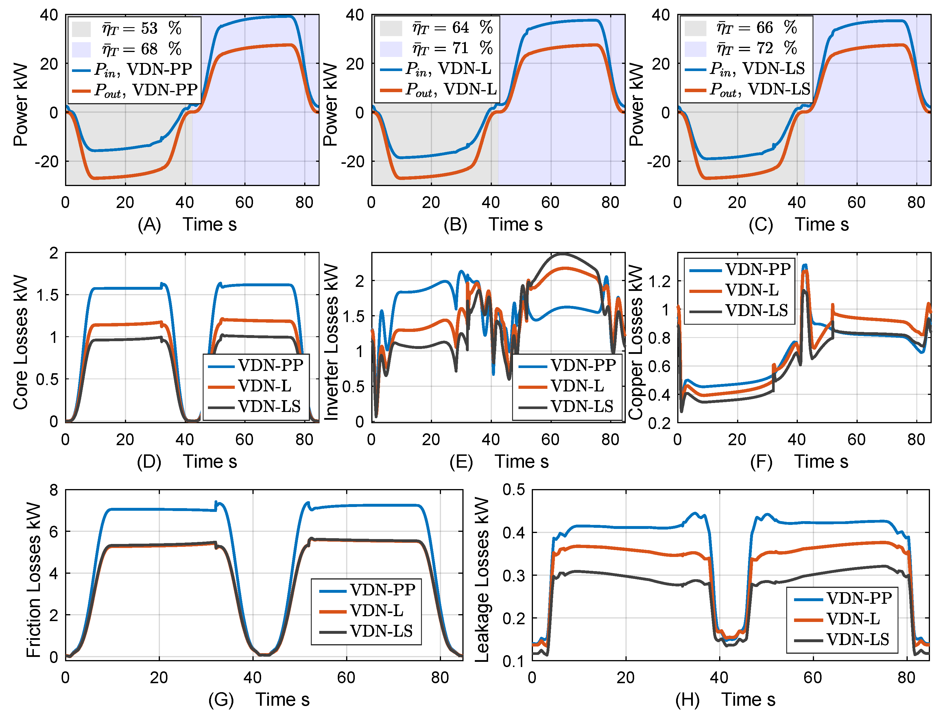
For comparison, the efficiency maps for the crane actuated by the VDN-PP, VDN-L, and VDN-LS appear as depicted in Figure 18, Figure 19 and Figure 20, respectively. The load cycle considered here allows for energy regeneration for the VDN’s; however, the obtained efficiencies differ from topology to topology. For the VDN-PP, all electric motors need to operate near their nominal speeds to realize the functionality, whereas the VDN-L and VDN-LS are not due to the hydraulic interconnections between the chambers of the two cylinders. Hence, the increased efficiencies due to lower speed dependent losses. Furthermore, due to the shared chambers of the VDN-LS, no VsD losses are associated with hydraulic power exchange between chambers 2 and 3 as opposed to the VDN-L, resulting in a relative increase in efficiency in this case. As the efficiency of the valve solution is zero during payload extension, it is not sensible to compare efficiencies for this part of the load case. During payload retraction, on the other hand, the increase in average efficiency is 59 [%], 66 [%], and 68 [%] for the VDN-PP, VDN-L, and VDN-LS, respectively. Furthermore, the ideal installed power required is reduced by 24 [%], 18 [%], and 22 [%] for the VDN-PP, VDN-L, and VDN-LS, respectively, when compared to the valve solution.

4.7.2. Performance and Energy Savings for Typical Crane Load Cycle

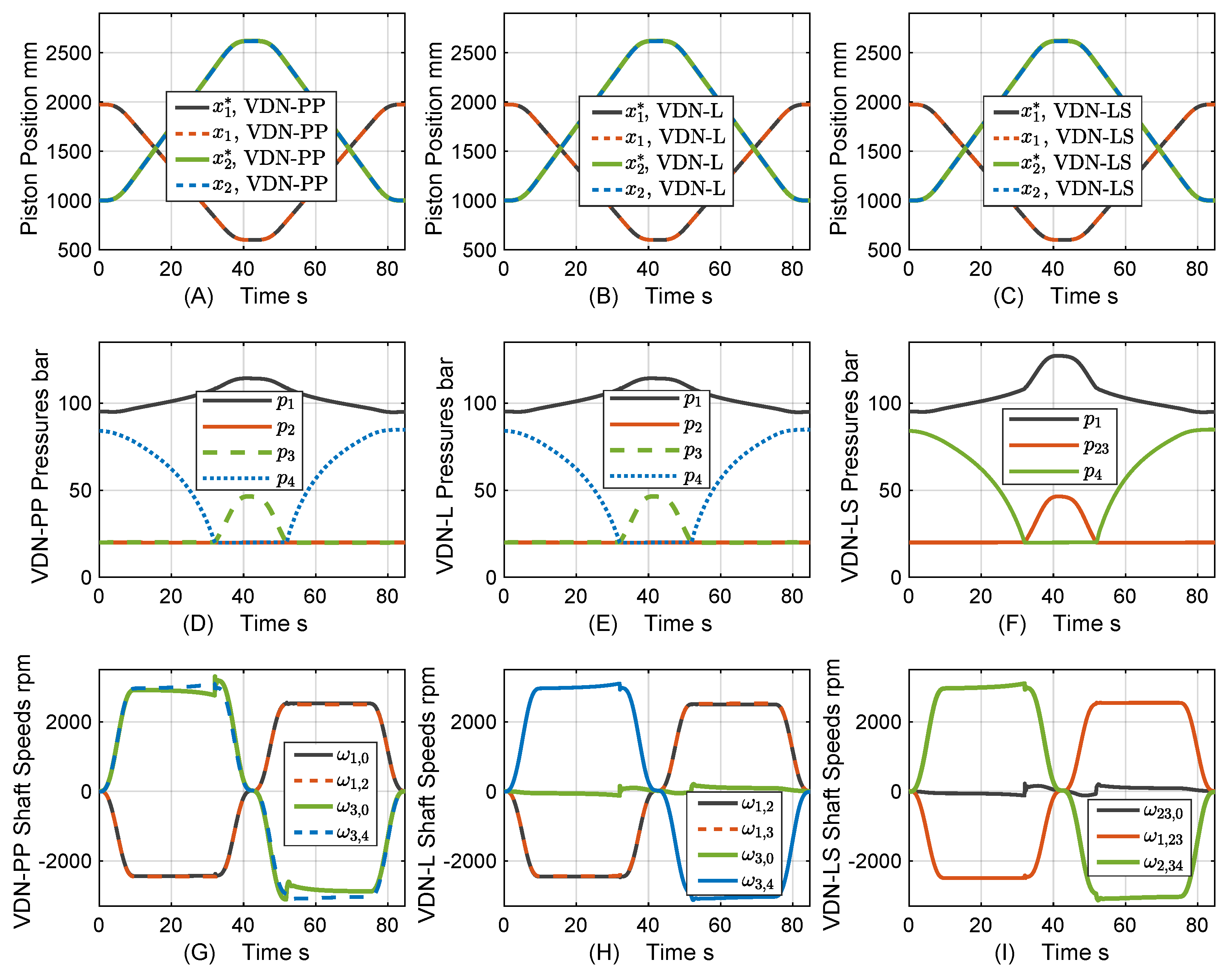
The VDN performances for a typical load case, where the load is moved away and subsequently towards the crane base, are illustrated in Figure 21 (simulation results). From the Figure 21A–F, all VDN’s considered demonstrate similar motion control performance and the lower chamber pressures are maintained in close proximity of the lower pressure setting of 20 bar by their sum pressure controls. Whereas the VDN-PP and VDN-L chamber pressures closely resemble each other, the shared chambers of the VDN-LS cause the pressure in chamber 2 to exceed the lower pressure setting as dictated by the required pressure in chamber 3. Consequently, the pressure in chamber 1 increases due to the load force. Furthermore, from Figure 21G–I, it is notable that the tank interconnecting VsD’s of the VDN-L and VDN-LS operate at low speeds due to VsD interconnections between the chambers of cylinders 1 and 2. As such interconnections are not present for VDN-PP, all its motors need to operate near their nominal speeds concurrently.

The corresponding input and output powers as well as the individual loss components at VDN level are depicted in Figure 22. By inspection, the main reasons for the improved efficiencies of the VDN-L and VDN-LS over the VDN-PP are associated with the speed dependent friction and core losses, whereas the copper and inverter losses are especially somewhat similar for all VDN’s. Indeed, the lower friction and core losses for the VDN-L and VDN-LS are a result of the tank interconnecting VsD’s generally running at lower speeds. In addition, the shared chambers of the VDN-LS eliminate the VsD losses otherwise associated with the VsD interconnecting chambers 2 and 3 as for the VDN-L.

4.8. Case Study Summary

The installed power for the VDN-PP, VDN-L, and VDN-LS was found to 68.49 [kW], 76.65 [kW], and 72.88 [kW], respectively, whereas it was found to 93.31 [kW] for the valve actuated solution. In comparison to the valve solution, there are yield reductions of 27 [%], 18 [%], and 22 [%] for the VDN-PP, VDN-L, and VDN-LS, respectively. Even though the VDN-PP here exhibits the lowest installed power, the lower power consumption and fewer components may render the VDN-LS the more attractive solution.

5. Conclusions

The idea of electro-hydraulic variable-speed drive networks is introduced, essentially constituting interconnected multi-cylinder/motor drives. These interconnections are established on both the electrical side as well as on the hydraulic side, enabling the main drive functionalities without any throttle control. As opposed to standalone electro-hydraulic variable-speed drives, this allows for distributing power directly between cylinder/motor, limiting the level of power conversions (electric-to-hydraulic/hydraulic-to-electric). Inspired by communication theory, six basic drive network topologies are introduced, and subsequently network topologies with shared/short circuited cylinder chambers exemplified. Perspectives on electro-hydraulic variable-speed drive networks are discussed, including design considerations, integration of hydraulic storages, drive compactness, and control designs.

In order to illuminate potential design approaches for electro-hydraulic variable-speed drive networks, a case study on a crane application is considered including three different electro-hydraulic variable-speed drive network topologies. Related design considerations demonstrate that numerous unique architectures exist for each network topology, even for a dual cylinder application, and that care must be taken in the architecture design phase in order to obtain the most feasible one. The cylinder/motor interconnections realized with electro-hydraulic variable-speed drive networks cause drive control designs to be non-trivial, and a decoupling control approach is proposed in combination with motion controls. The proposed drive controls allow for individual control of cylinder/motor motion/force, while controlling the sum pressure(s) and through this the lower chamber pressure(s) of the drive networks. Furthermore, the case study reveals that electro-hydraulic variable-speed drive networks allow for significant energy efficiency increases compared to a valve solution. In addition, higher energy efficiencies are found for electro-hydraulic variable-speed drive networks with interconnections across actuator chambers as compared to cases where actuators are only interconnected on the electric side. Whereas the required motor power to be installed is somewhat similar for the case study, short circuiting of chambers allows for reducing the number of variable-speed displacement units, hence enabling a reduction of component integration costs.

In summary, electro-hydraulic variable-speed drive networks are believed to possess significant potentials in the ongoing electrification transformation throughout many industry segments. This is owed to the vast amount of unique drive network architectures encompassed by electro-hydraulic variable-speed drive network topologies and potentially large energy savings compared to existing valve and variable-speed drive technologies.

References

- Scheidl, R.; Gradl, C.; Kogler, H.; Foschum, P.; Plöckinger, A. Investigation of a Switch-Off Time Variation Problem of a Fast Switching Valve. In Proceedings of the ASME/BATH 2014 Symposium on Fluid Power and Motion Control, Bath, UK, 10–12 September 2014; ASME: Bath, UK; p. V001T01A033. [Google Scholar] [CrossRef]
- Roemer, D.; Johansen, P.; Schmidt, L.; Andersen, T. Modeling of movement-induced and flow-induced fluid forces in fast switching valves. In Proceedings of the 2015 International Conference on Fluid Power and Mechatronics (FPM), Harbin, China, 5–7 August 2015; pp. 978–983. [Google Scholar] [CrossRef]
- Kogler, H.; Scheidl, R.; Schmidt, B.H. Analysis of Wave Propagation Effects in Transmission Lines due to Digital Valve Switching. In Proceedings of the ASME/BATH 2015 Symposium on Fluid Power and Motion Control, Chicago, IL, USA, 12–14 October 2015; ASME: Bath, UK; p. V001T01A057. [Google Scholar] [CrossRef]
- Huova, M.; Linjama, M.; Siivonen, L.; Deubel, T.; Försterling, H.; Stamm, E. Novel Fine Positioning Method for Hydraulic Drives Utilizing On/Off-Valves. In Proceedings of the BATH/ASME 2018 Symposium on Fluid Power and Motion Control, Bath, UK, 12–14 September 2018; ASME: Bath, UK; p. V001T01A046. [Google Scholar] [CrossRef]
- Karvonen, M.; Heikkilä, M.; Tikkanen, S.; Linjama, M.; Huhtala, K. Aspects of the Energy Consumption of a Digital Hydraulic Power Management System Supplying a Digital and Proportional Valve Controlled Multi Actuator System. In Proceedings of the ASME/BATH 2014 Symposium on Fluid Power and Motion Control, Bath, UK, 10–12 September 2014; ASME: Bath, UK; p. V001T01A012. [Google Scholar] [CrossRef]
- Midgley, W.J.; Abrahams, D.; Garner, C.P.; Caldwell, N. Modelling and experimental validation of the performance of a digital displacement® hydraulic hybrid truck: Proceedings of the Institution of Mechanical Engineers, Part D. J. Automob. Eng. 2022, 236, 594–605. [Google Scholar] [CrossRef]
- Rampen, W.; Dumnov, D.; Taylor, J.; Dodson, H.; Hutcheson, J.; Caldwell, N. A Digital Displacement Hydrostatic Wind-turbine Transmission. Int. J. Fluid Power 2021, 21, 87–112. [Google Scholar] [CrossRef]
- MacPherson, J.; Williamson, C.; Green, M.; Caldwell, N. Energy efficient excavator hydraulic systems with digital displacement® pump-motors and digital flow distribution. In Proceedings of the BATH/ASME 2020 Symposium on Fluid Power and Motion Control, Bath, UK, 9–11 September 2020; ASME: Bath, UK; p. V001T01A035. [Google Scholar] [CrossRef]
- Hutcheson, J.; Abrahams, D.; MacPherson, J.; Caldwell, N.; Rampen, W. Demonstration of efficient energy recovery systems using digital displacement® hydraulics. In Proceedings of the BATH/ASME 2020 Symposium on Fluid Power and Motion Control, Bath, UK, 9–11 September 2020; ASME: Bath, UK; p. V001T01A033. [Google Scholar] [CrossRef]
- Budden, J.J.; Williamson, C. Danfoss Digital Displacement® Excavator: Test results and analysis. In Proceedings of the ASME/BATH 2019 Symposium on Fluid Power and Motion Control, Longboat Key, FL, USA, 7–9 October 2019; ASME: Bath, UK; p. V001T01A032. [Google Scholar] [CrossRef]
- Pedersen, N.H.; Johansen, P.; Schmidt, L.; Scheidl, R.; Andersen, T.O. Control and performance analysis of a digital direct hydraulic cylinder drive. Int. J. Fluid Power 2019, 20, 295–322. [Google Scholar] [CrossRef]
- Zagar, P.; Kogler, H.; Scheidl, R.; Winkler, B. Hydraulic Switching Control Supplementing Speed Variable Hydraulic Drives. Actuators 2020, 9, 129. [Google Scholar] [CrossRef]
- Hansen, A.H.; Asmussen, M.F.; Bech, M.M. Hardware-in-the-loop Validation of Model Predictive Control of a Discrete Fluid Power Take-Off System for Wave Energy Converters. Energies 2019, 12, 3668. [Google Scholar] [CrossRef] [Green Version]
- Hansen, A.H.; Asmussen, M.F.; Bech, M.M. Model Predictive Control of a Wave Energy Converter with Discrete Fluid Power Take-Off System. Energies 2018, 11, 635. [Google Scholar] [CrossRef] [Green Version]
- Pedersen, N.H.; Johansen, P.; Andersen, T.O. Feedback Control of Pulse-Density-Modulated Digital Displacement Transmission Using a Continuous Approximation. IEEE/ASME Trans. Mechatronics 2020, 25, 2472–2482. [Google Scholar] [CrossRef]
- Jensen, K.J.; Ebbesen, M.K.; Hansen, M.R. Novel Concept for Electro-Hydrostatic Actuators for Motion Control of Hydraulic Manipulators. Energies 2021, 14, 6566. [Google Scholar] [CrossRef]
- Padovani, D.; Ketelsen, S.; Hagen, D.; Schmidt, L. A Self-Contained Electro-Hydraulic Cylinder with Passive Load-Holding Capability. Energies 2019, 12, 292. [Google Scholar] [CrossRef] [Green Version]
- Imam, A.; Rafiq, M.; Jalayeri, E.; Sepehri, N. Design, Implementation and Evaluation of a Pump-Controlled Circuit for Single Rod Actuators. Actuators 2017, 6, 10. [Google Scholar] [CrossRef] [Green Version]
- Michel, S.; Weber, J. Energy-efficient electrohydraulic compact drives for low power applications. In Proceedings of the BATH 2012 Symposium on Fluid Power and Motion Control, FPMC, Bath, UK, 12–14 September 2012. [Google Scholar]
- Çalışkan, H.; Balkan, T.; Platin, B.E. A Complete Analysis and a Novel Solution for Instability in Pump Controlled Asymmetric Actuators. J. Dyn. Syst. Meas. Control 2015, 137, 091008. [Google Scholar] [CrossRef]
- Weber, J.; Beck, B.; Fischer, E.; Ivantysyn, R.; Kolks, G.; Kunkis, M.; Lohse, H.; Lübbert, J.; Michel, S.; Schneider, M.; et al. Novel System Architectures by Individual Drives. In Proceedings of the 10th International Fluid Power Conference (IFK), Dresden, Germany, 8–10 May 2016. [Google Scholar]
- Wiens, T.; Deibert, B. A low-cost miniature electrohydrostatic actuator system. Actuators 2020, 9, 130. [Google Scholar] [CrossRef]
- Stawinski, L.; Skowronska, J.; Kosucki, A. Energy Efficiency and Limitations of the Methods of Controlling the Hydraulic Cylinder Piston Rod under Various Load Conditions. Energies 2021, 14, 7973. [Google Scholar] [CrossRef]
- Agostini, T.; Negri, V.D.; Minav, T.; Pietola, M. Effect of energy recovery on efficiency in electro-hydrostatic closed system for differential actuator. Actuators 2020, 9, 12. [Google Scholar] [CrossRef] [Green Version]
- Zhang, S.; Li, S.; Minav, T. Control and Performance Analysis of Variable Speed Pump-Controlled Asymmetric Cylinder Systems under Four-Quadrant Operation. Actuators 2020, 9, 123. [Google Scholar] [CrossRef]
- Casoli, P.; Scolari, F.; Minav, T.; Rundo, M. Comparative energy analysis of a load sensing system and a zonal hydraulics for a 9-tonne excavator. Actuators 2020, 9, 39. [Google Scholar] [CrossRef]
- Schmidt, L.; Ketelsen, S.; Grønkær, N.; Hansen, K.V. On Secondary Control Principles in Pump Controlled Electro-Hydraulic Linear Actuators. In Proceedings of the BATH/ASME 2020 Symposium on Fluid Power and Motion Control, Bath, UK, 9–11 September 2020; ASME: Bath, UK; p. V001T01A009. [Google Scholar] [CrossRef]
- Schmidt, L.; Ketelsen, S.; Padovani, D.; Mortensen, K.A. Improving the efficiency and dynamic properties of a flow control unit in a self-locking compact electro-hydraulic cylinder drive. In Proceedings of the ASME/BATH 2019 Symposium on Fluid Power and Motion Control, Longboat Key, FL, USA, 7–9 October 2019; ASME: Bath, UK; p. V001T01A034. [Google Scholar] [CrossRef]
- Schmidt, L.; Ketelsen, S.; Brask, M.H.; Mortensen, K.A. A Class of Energy Efficient Self-Contained Electro-Hydraulic Drives with Self-Locking Capability. Energies 2019, 12, 1866. [Google Scholar] [CrossRef] [Green Version]
- Schmidt, L.; Groenkjaer, M.; Pedersen, H.C.; Andersen, T.O. Position Control of an Over-Actuated Direct Hydraulic Cylinder Drive. Control Eng. Pract. 2017, 64, 1–14. [Google Scholar] [CrossRef]
- Ketelsen, S.; Schmidt, L.; Donkov, V.H.; Andersen, T.O. Energy Saving Potential in Knuckle Boom Cranes using a Novel Pump Controlled Cylinder Drive. Model. Identif. Control 2018, 39, 73–89. [Google Scholar] [CrossRef] [Green Version]
- Schmidt, L.; Roemer, D.B.; Pedersen, H.C.; Andersen, T.O. Speed-variable switched differential pump system for direct operation of hydraulic cylinders. In Proceedings of the ASME/BATH 2015 Symposium on Fluid Power and Motion Control, Chicago, IL, USA, 12–14 October 2015; ASME: Bath, UK; p. V001T01A042. [Google Scholar] [CrossRef]
- Helduser, S. Hydraulische Antriebssysteme mit drehzahlverstellbarer pumpe. Ölhydraulik Pneum. 1997, 41, 30. [Google Scholar]
- Helduser, S. Electric-Hydrostatic Drive Systems and their Application in Injection Moulding Machines. In Proceedings of the 4th JFPS International Symposium; The Japan Fluid Power System Society: Tokyo, Japan, 1999; Volume 41, pp. 261–266. [Google Scholar] [CrossRef]
- Ketelsen, S.; Andersen, T.O.; Ebbesen, M.K.; Schmidt, L. Mass Estimation of Self-contained Linear Electro-hydraulic Actuators and Evaluation of the Influence on Payload Capacity of a Knuckle Boom Crane. In Proceedings of the ASME/BATH 2019 Symposium on Fluid Power and Motion Control, Longboat Key, FL, USA, 7–9 October 2019; ASME: Bath, UK; p. V001T01A045. [Google Scholar] [CrossRef]
- Ketelsen, S.; Michel, S.; Andersen, T.O.; Ebbesen, M.K.; Weber, J.; Schmidt, L. Thermo-hydraulic modelling and experimental validation of an electro-hydraulic compact drive. Energies 2021, 14, 2375. [Google Scholar] [CrossRef]
- Ketelsen, S.; Andersen, T.O.; Ebbesen, M.K.; Schmidt, L. A self-contained cylinder drive with indirectly controlled hydraulic lock. Model. Identif. Control 2020, 41, 185–205. [Google Scholar] [CrossRef]
- Padovani, D.; Ketelsen, S.; Schmidt, L. Downsizing the Electric Motors of Energy-efficient Self-contained Electro-hydraulic Systems by Using Hybrid Technologies. In Proceedings of the BATH/ASME 2020 Symposium on Fluid Power and Motion Control, Virtual, Online, 9–11 September 2020; ASME: Bath, UK; p. V001T01A005. [Google Scholar] [CrossRef]
- Qu, S.; Fassbender, D.; Vacca, A.; Busquets, E. A cost-effective electro-hydraulic actuator solution with open circuit architecture. Int. J. Fluid Power 2021, 22, 233–258. [Google Scholar] [CrossRef]
- Qu, S.; Fassbender, D.; Vacca, A.; Busquets, E. A high-efficient solution for electro-hydraulic actuators with energy regeneration capability. Energy 2021, 216, 119291. [Google Scholar] [CrossRef]
- Qu, S.; Fassbender, D.; Vacca, A.; Busquets, E. Development of a Lumped-Parameter Thermal Model for Electro-Hydraulic Actuators. In Proceedings of the 10th International Conference on Fluid Power Transmission and Control (ICFP 2021), Hangzhou, China, 11–13 April 2021. [Google Scholar]
- Padovani, D. Leveraging Flow Regeneration in Individual Energy-Efficient Hydraulic Drives. In Proceedings of the ASME/BATH 2021 Symposium on Fluid Power and Motion Control, Virtual, Online, 19–21 October 2021; ASME: Bath, UK; p. V001T01A013. [Google Scholar] [CrossRef]
- Ketelsen, S.; Padovani, D.; Andersen, T.; Ebbesen, M.; Schmidt, L. Classification and Review of Pump-Controlled Differential Cylinder Drives. Energies 2019, 12, 1293. [Google Scholar] [CrossRef] [Green Version]
- Fassbender, D.; Zakharov, V.; Minav, T. Utilization of electric prime movers in hydraulic heavy-duty-mobile-machine implement systems. Autom. Constr. 2021, 132, 103964. [Google Scholar] [CrossRef]
- Busquets, E. An Investigation of the Cooling Power Requirements for Displacement-Controlled Multi-Actuator Machines. Ph.D. Thesis, Purdue University, West Lafayette, IN, USA, 2013. [Google Scholar]
- Busquets, E.; Ivantysynova, M. A Multi-Actuator Displacement-Controlled System with Pump Switching—A Study of the Architecture and Actuator-Level Control. JFPS Int. J. Fluid Power Syst. 2015, 8, 66–75. [Google Scholar] [CrossRef] [Green Version]
- Li, P.Y.; Siefert, J.; Bigelow, D. A hybrid hydraulic-electric architecture (HHEA) for high power off-road mobile machines. In Proceedings of the ASME/BATH 2019 Symposium on Fluid Power and Motion Control, Longboat Key, FL, USA, 7–9 October 2019; ASME: Bath, UK; p. V001T01A011. [Google Scholar] [CrossRef]
- Siefert, J.; Li, P.Y. Optimal Operation of a Hybrid Hydraulic Electric Architecture (HHEA) for Off-Road Vehicles over Discrete Operating Decisions. In Proceedings of the 2020 American Control Conference (ACC), Denver, CO, USA, 1–3 July 2020; pp. 3255–3260. [Google Scholar] [CrossRef]
- Siefert, J.; Li, P.Y. Optimal control and energy-saving analysis of common pressure rail architectures: HHEA & STEAM. In Proceedings of the BATH/ASME 2020 Symposium on Fluid Power and Motion Control, Virtual, Online, 9–11 September 2020; ASME: Bath, UK; p. V001T01A050. [Google Scholar] [CrossRef]
- Khandekar, A.; Wills, J.; Wang, M.; Li, P.Y. Incorporating Valve Switching Losses into a Static Optimal Control Algorithm for the Hybrid Hydraulic-Electric Architecture (HHEA). In Proceedings of the ASME/BATH 2021 Symposium on Fluid Power and Motion Control, Virtual, Online, 9–21 October 2021; ASME: Bath, UK; p. V001T01A046. [Google Scholar] [CrossRef]
- Fassbender, D.; Minav, T.; Brach, C.; Huhtala, K. Improving the Energy Efficiency of Single Actuators with High Energy Consumption: An Electro-Hydraulic Extension of Conventional Multi-Actuator Load-Sensing Systems. In Proceedings of the Scandinavian International Conference on Fluid Power, Linköping, Sweden, 31 May–2 June 2021; pp. 74–89. [Google Scholar]
- Forouzan, B.A. Forouzan. Data Communications and Networking, 4th ed.; McGraw-Hill, McGraw-Hill Companies Inc.: New York, NY, USA, 2007; ISBN 13 978-0-07-296775-3. [Google Scholar]
- Rühlicke, I. Elektrohydraulische Antriebssysteme mit Drehzahlveränderbarer Pumpe. Ph.D. Thesis, TU Dresden, Dresden, Germany, 1997. [Google Scholar]
- Neubert, T. Elektro-hydraulische antriebssysteme mit drehzahlveränderbaren Pumpen. Int. Fluidtechnisches Kolloqu. Aachen 1998, 1, 17–18. [Google Scholar]
- Helduser, S. Electric-hydrostatic drive—An innovative energy-saving power and motion control system. Proc. Inst. Mech. Eng. Part I J. Syst. Control Eng. 1999, 213, 427–437. [Google Scholar] [CrossRef]
- Neubert, T. Untersuchungen von Drehveränderbaren Pumpen. Ph.D. Thesis, RWTH Aachen, Aachen, Germany, 2002. [Google Scholar]
- Quan, L.; Neubert, T.; Helduser, S. Principle to closed loop control differential cylinder wit double speed variable pumps and single loop control signal. Chin. J. Mech. Eng. 2004, 17, 85–88. [Google Scholar] [CrossRef]
- U.S. Department of Energy, Advanced Manufacturing Office. Adjustable Speed Drive Part-Load Efficiency; U.S. Department of Energy, Advanced Manufacturing Office: Washington, DC, USA, 2012.
- Innas, B.V. Performance of Hydrostatic Machines—Extensive Measurement Report. Technical Report. 2020. Available online: https://www.innas.com/assets/performance-of-hydrostatic-machines.pdf (accessed on 13 January 2022).
- Schmidt, L.; Ketelsen, S.; Mommers, R.; Achten, P. Analogy between hydraulic transformers & variable-speed pumps. In Proceedings of the BATH/ASME 2020 Symposium on Fluid Power and Motion Control, Virtual, Online, 9–11 September 2020; ASME: Bath, UK; p. V001T01A007. [Google Scholar] [CrossRef]
- Bosch Rexroth AG. MS2N Synchronous Servomotors Project Planning Manual R911347583, Edition 05. 2020. Available online: https://www.boschrexroth.com/documents/12605/33006371/R91134758307.pdf/43fe3dca-0606-f4b7-03ab-b0e63944cbe3 (accessed on 13 January 2022).