
An Effective Numerical Simulation Method for Steam Injection Assisted In Situ Recovery of Oil Shale

1
State Key Laboratory of Shale Oil and Gas Enrichment Mechanisms and Effective Development, Beijing 100083, China
2
State Center for Research and Development of Oil Shale Exploitation, Beijing 100083, China
3
Key Laboratory of Drilling and Production Engineering for Oil and Gas, Wuhan 430100, China
*
Author to whom correspondence should be addressed.
Energies 2022, 15(3), 776; https://0-doi-org.brum.beds.ac.uk/10.3390/en15030776
Submission received: 2 December 2021
/
Revised: 10 January 2022
/
Accepted: 18 January 2022
/
Published: 21 January 2022
(This article belongs to the Special Issue Shale Oil and Gas Accumulation Mechanism)
Abstract
:This paper presents an effective numerical simulation method for production prediction of in situ recovery of oil shale reservoirs with steam injection. In this method, finite volume-based discretization schemes of heat and mass transfer equations of the thermal compositional model are derived and used. The embedded discrete fracture model is used to accurately handle the fractured vertical well. A smooth non-linear solver is proposed to solve the global equations, then cell pressure, temperature, saturation, component mole fractions, and well production rates can be obtained. Compared with the existing commercial software, this new method can have a smoother non-linear solution and handle the complex fracture geometry theoretically. A numerical example is used to test this presented method and can realize accurate calculation results compared with CMG. Another numerical case with a hydraulic fracture and an open thermal boundary condition is implemented to validate the presented method and can effectively handle the actual situation of steam injection-assisted in situ recovery of oil shale, which was difficult to handle using previous methods.
1. Introduction
The world is rich in oil shale resources, and against the background of the increasing shortage of traditional oil resources, the efficient exploitation of oil shale becomes increasingly important. The kinetic reaction of oil shale is the key factor for oil shale production, which had been widely modeled [1,2,3]. Up to now, the relatively mature oil-shale in situ production technologies have been microwave heating technology [4], electric heating technology, and fluid heating technology.
Since the Shell company successfully developed electric heating technology and conducted field tests, the technology has been widely recognized by the public, and the numerical simulation analysis of the technology has been widely studied. Harold and Scott [5] used the commercial software Computer Modeling Group (CMG) STARS module to simulate the electric-heating in situ production process in an oil field in northwest Colorado, simulated and calculated the oil and gas production, and compared it with the actual production data. Fan et al. [6] simulated the process of oil shale pyrolysis and pyrolysis product seepage by electric heater heating oil shale based on the Stanford General Purpose Research simulator (GPRS). Shen et al. [7] also used the stars module of CMG, considered the wellbore reflux heat loss and skin effect, simulated the field process of shell oil shale electric heating, and achieved higher calculation accuracy of production data.
Compared with the electric-heating in situ recovery technology, the fluid-assisted in situ recovery technology of oil shale is more complex [8]. More factors need to be considered in its numerical simulation, including heat transfer, temperature field, pressure field, fluid field, and the influence of fractures. Pei et al. [9] studied the mechanism of nitrogen injection-assisted in situ recovery of oil shale. The steam injection can provide more heat to the formation, and compared with the only heat conduction effect in electric heating, the thermal convection effect of steam injection in the formation can achieve more efficient heat transfer, so as to effectively improve the oil shale recovery in theory. Wang et al. [10] made a numerical study of the actual field case of in situ recovery of oil shale by injecting superheated steam. Due to the low permeability of the oil shale matrix, steam injection is often carried out by fractured vertical wells, so handling the hydraulic fracture is a key factor in steam injection-assisted oil shale recovery. Taheri et al. [11] studied the effect of hydraulic fracture characteristics on the thermal EOR process. The embedded discrete fracture model (EDFM) [12,13,14] or distinct element method [15] is an effective method to efficiently handle the large-scale discrete fracture.
A compositional model is generally used to model the in situ recovery of oil shale. In the compositional model by Fan et al. [6], the chemical reaction of kerogen decomposition, component phase equilibrium, multiphase seepage and thermal convection diffusion are considered, and the equations are solved by a fully implicit Newton iterative method. Li et al. [16,17] proposed a multi-scale numerical simulation method for oil shale in situ mining in view of the slow calculation efficiency of oil shale numerical simulation. Zheng et al. [18] used a simplified compositional model and combined the experimental data for a kinetic reaction of oil shale to study the production process of in situ combustion of oil shale. Multi-physics coupled simulation studies for oil shale recovery were also implemented to make the production prediction more accurate [19,20].
At present, there is no relevant research on the numerical model of steam injection via a fractured vertical well for oil shale production based on a thermal compositional model, so the numerical simulation of oil shale in situ production is still undergoing further research. Based on the thermal compositional model, the finite volume method, embedded discrete fracture model, and a smooth non-linear solver of the thermal compositional model without judging phase change, this paper intends to form an effective numerical simulation method of steam injection assisted in situ recovery of oil shale, to provide an efficient and accurate production prediction.
2. Methodology
2.1. Basic Thermal Compositional Model for Oil Shale Recovery
The numerical simulation of in situ recovery of oil shale involves the coupling calculation of heat and mass transfer equation based on a kerogen pyrolysis chemical reaction, so it is a more complex thermal compositional model. It mainly includes the mass conservation equation, energy conservation equation of each component, and the auxiliary equation composed of a phase equilibrium equation and well equation. It should be pointed out that in order to reduce the difficulty of calculation and improve the calculation efficiency, constant values that do not change with the component concentration are adopted for the physical properties of each phase in this paper, and it can be understood as the average of these physical properties of each phase in the whole calculation process. The relevant equations are introduced as follows:
- (1)
- Mass conservation equations
For fluid components:
where fluid components include six types: CO2, N2, HO2, C2, C13, C37, and .
For the components in the solid phase, there are two components, kerogen, and coke. For kerogen, the mass conservation equation is:
where .
For coke, due to coke being generally not the product of the chemical reaction, the equation is:
where is the coke concentration in the solid phase.
- (2)
- Energy conservation equation:
- (3)
- Auxiliary equation
Chemical reaction model:
where is the kerogen concentration in the solid phase, because the kerogen is generally the only reactant.
In the in situ recovery of oil shale, the phase equilibrium of each fluid component in oil phase and gas phase is considered.
Phase equilibrium model:
Well model:
where .
where .
2.2. Finite Volume-Based Discretization of Governing Equations
In this paper, the above equations are discretized based on the block-center finite volume method. Taking the mass conservation equation of fluid components as an example, the finite volume discrete scheme of the governing equation is derived in detail as follows:
For the control volume Vh of the h-th grid, assuming that there are nm grids adjacent to the grid, then take the time and volume integration of both sides of Equation (1) to obtain:
The right side of the above equation is rewritten as:
Then the integration is furtherly approximated as:
where .
The second term at the left side of Equation (9) is estimated by a Gaussian formula, and the following is obtained:
The two-point linear approximation scheme of interface flux is used to further estimate the right side of Equation (13) as:
where is the transmissibility of phase j between grid m and grid k, which is equal to the product of j-th phase mobility and geometric factor, that is:
For two adjacent rectangular grids, the geometric factor is calculated as:
where and are the permeability of grid h and grid k respectively, and are the area of the interface of grid h and grid k.
The mobility is calculated as:
where the terms related to saturation (relative permeability) adopt an upstream weight scheme, and the terms related to pressure adopts an arithmetic average scheme, which are:
Then, Equation (14) is rewritten as:
The implicit scheme is used and the following are obtained:
Then combining Equations (22)–(24), it is obtained that:
Similarly, for kerogen in the solid phase, the discrete scheme of Equation (2) can be obtained as:
For coke in the solid phase, the discrete scheme of Equation (3) is:
The discrete scheme for energy conservation equation can be obtained as:
where, is the enthalpy of the j-th phase between the h-th and k-th grids, which adopts the upstream weight scheme, i.e.,
2.3. Treatment of Hydraulic Fracture
Because the permeability of oil shale is very low, it is difficult to directly inject hot steam into oil shale reservoir, so the method of fracturing a vertical well is often used to inject hot steam. When fracturing vertical wells are used, the injected hot steam will flow along the high-conductivity fractures and then into the reservoir. Therefore, the numerical modeling of the flow in fractures is very important for the numerical simulation of steam injection assisted in situ production of oil shale. There have been lots of treatment methods for various fractures including hydraulic fractures, natural fractures, and induced fractures in the reservoir [21,22,23,24]. In this paper, due to the embedded discrete fracture model (EDFM) being easy to couple in the calculation of the thermal compositional model in the case of Cartesian mesh, the commonly used EDFM is used to explicitly handle the large-scale discrete fractures of fractured vertical wells [12,13,14]. The main idea is to embed discrete fractures into the Cartesian matrix grid, in which the transmissibility of phase j between matrix grid m and fracture grid f is:
where λj,mf is the mobility of the jth phase, and the upwind scheme is used. Gmf is:
where is the harmonic average value of fracture grid permeability and matrix grid permeability, and is the average distance from points in the matrix grid to the fracture grid.
2.4. Non-Linear Solver
The automatic differentiation-based Newton iteration method is generally used to solve the above non-linear equations. However, in the simulation of oil-shale in situ production, the initial condition of oil saturation is:
Therefore, it is necessary to judge whether there will be oil phase in each grid during the calculation process. If there is no oil phase, there is only a gas phase for each light and heavy component generated by oil shale pyrolysis, and the above phase equilibrium equation does not hold. If phase change occurs in a grid and oil phase is produced, the phase equilibrium equation between oil phase and gas phase just holds. Therefore, for different grids, generally, due to the different phase state, the equations within each grid may be different, which poses challenges to the smoothness of the non-linear calculation.
In order to enhance the smoothness of the Newton iteration-based solution process and improve the calculation efficiency without significantly reducing the calculation accuracy, the initial condition of oil saturation is set as:
To make each grid initially contain oil, the equations at the initial time of each grid are the same without judging in which grid the phase change occurs. Because there will be a residual saturation term in the relative permeability curve, that is, when the oil saturation in the grid is lower than that, the oil phase in the grid will not flow out if residual oil saturation meets:
It can be ensured that each grid will have at least oil saturation in the calculation process, so that there is no need to judge the phase change in the whole calculation process, and in each grid the control equations are the same, which improves the smoothness of the non-linear solution by Newton iteration.
In order to make the obtained solution by Newton iteration physical, some limiting equations need to be added to limit the concentration of each component in the range of 0–1, that is:
In this paper, the inequality constraint is transformed into an equality constraint and added to the global equations by introducing relaxation variables , that is,
Therefore, based on the block-center finite volume method that satisfies local mass conservation and using the two-point linear approximation scheme of the orthogonal grid, the 17 discrete equations are obtained, and there are also 17 independent variables, including: pressure, water saturation, gas saturation, solid-phase saturation, kerogen concentration in solid phase, temperature, concentration of five fluid components in gas phase except water components, and relaxation variables constrained by inequality.
2.5. Treatment of Boundary Condition
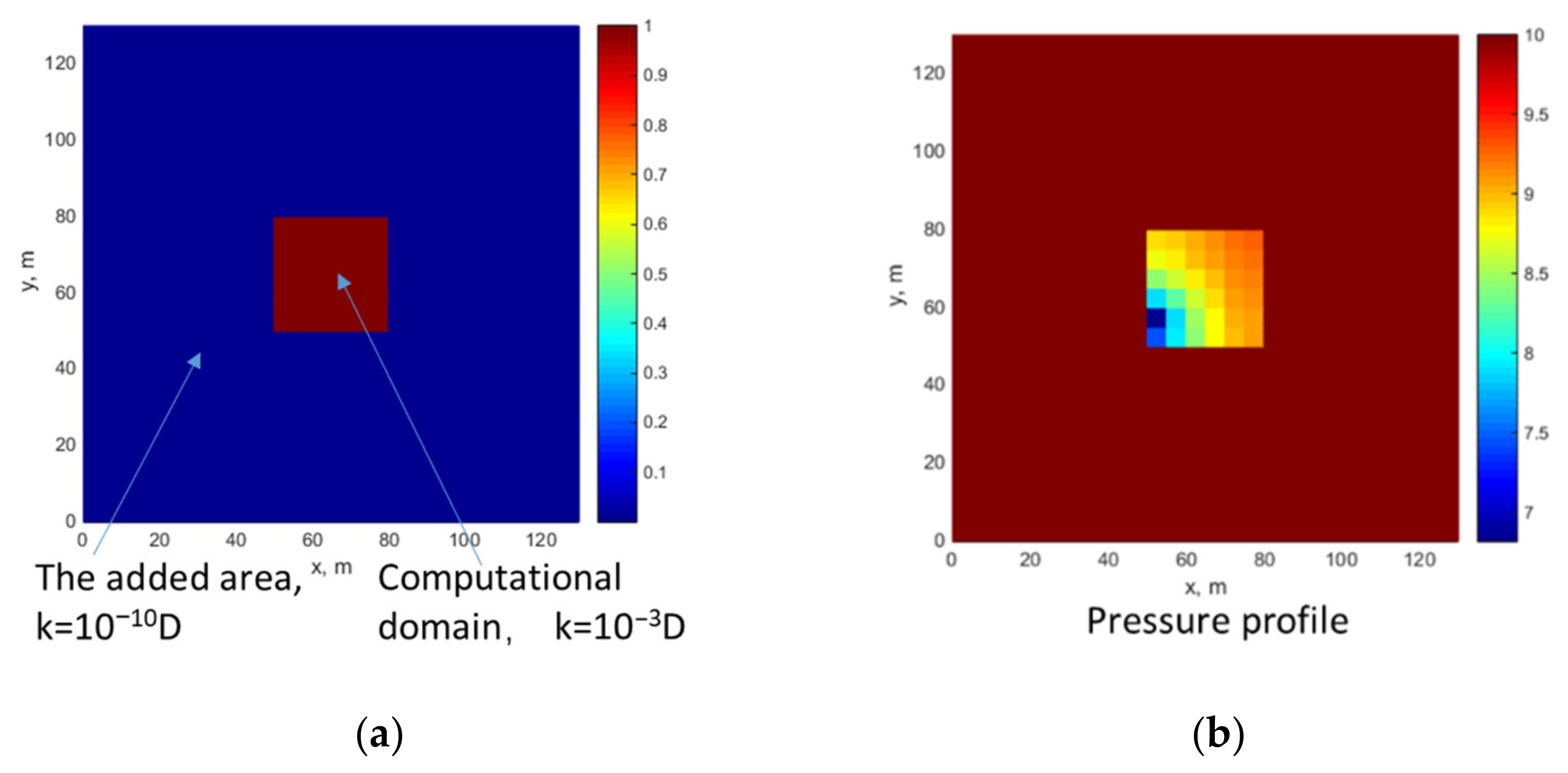
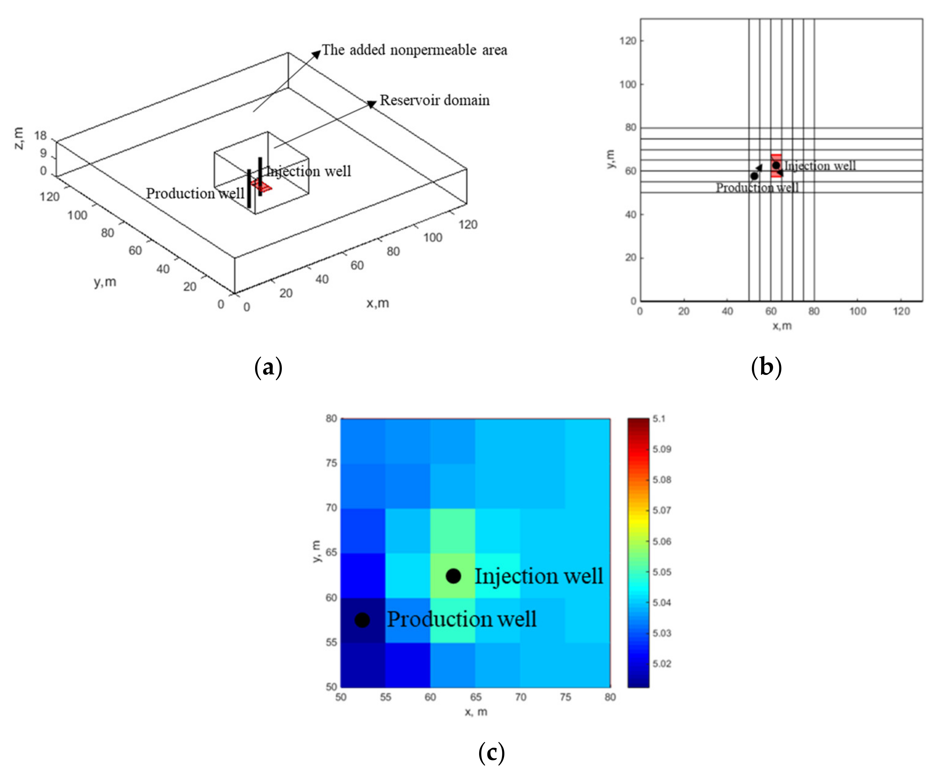
The reservoir boundary condition is closed, but it is still thermally conductive. In the commercial numerical simulator CMG, the boundary is closed, that is, there is neither mass transfer nor heat conduction. As shown in Figure 1a, the simulator achieves the purpose of little mass transfer but normal heat conduction by adding a circle of grid with extremely low permeability around the calculation domain, so as to form a more real reservoir boundary condition. In the pressure profile shown in Figure 1b, since the permeability of the grid added outside the calculation domain is very low, and the pressure of the grid added during the simulation calculation is always the initial reservoir pressure.
3. Numerical Examples
3.1. Validation of the Smooth Non-Linear Solver: A 2D Case with a Heater Device
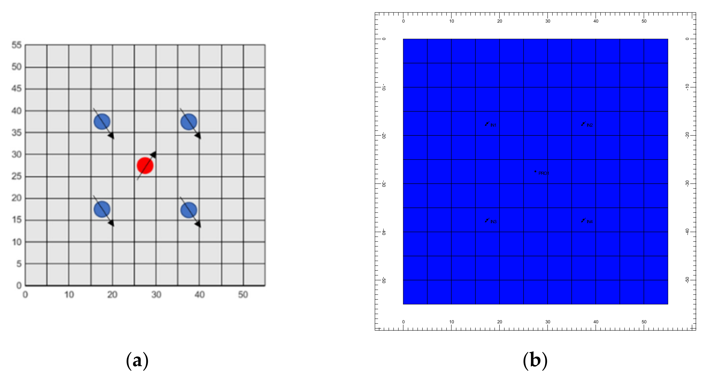
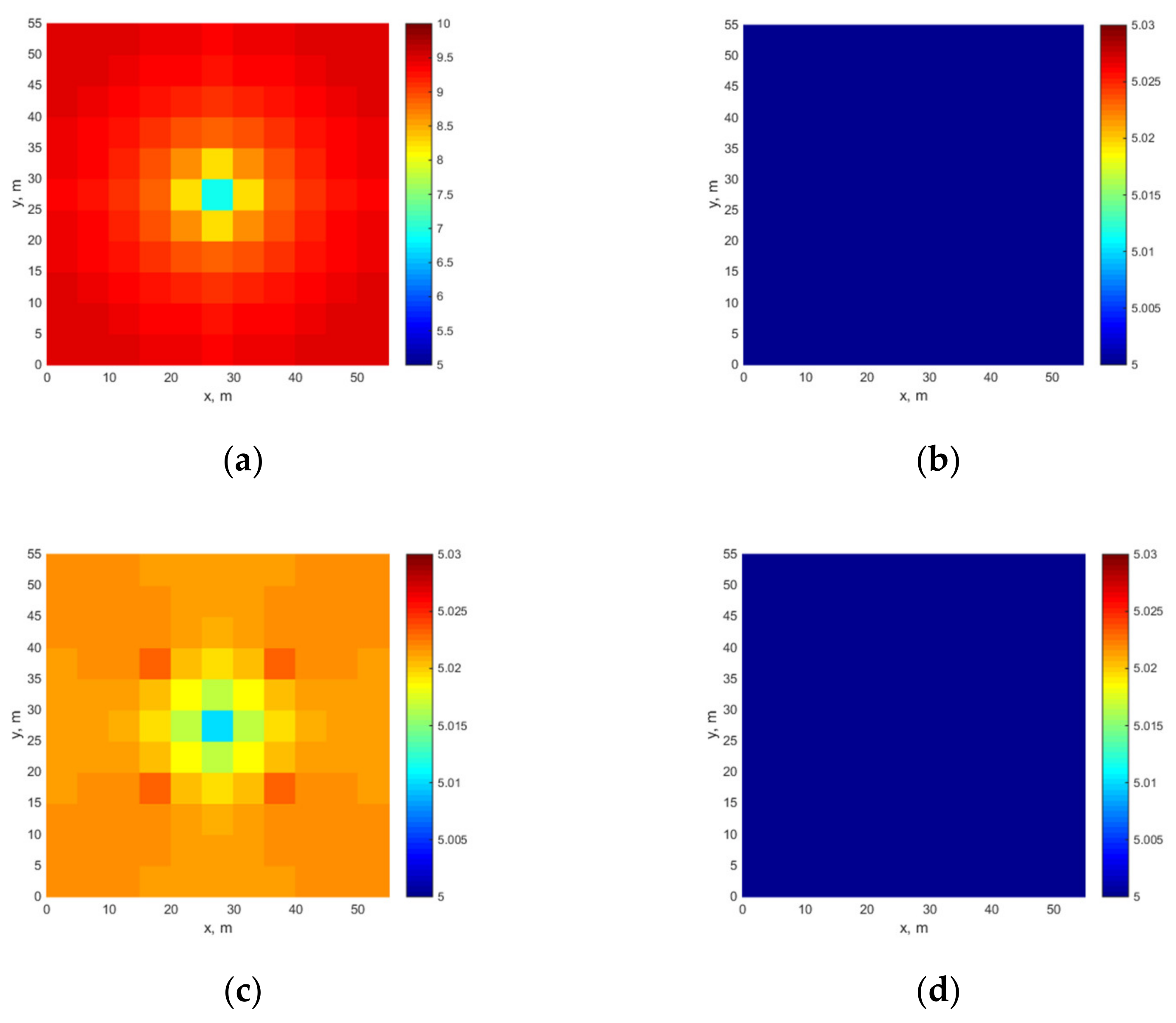
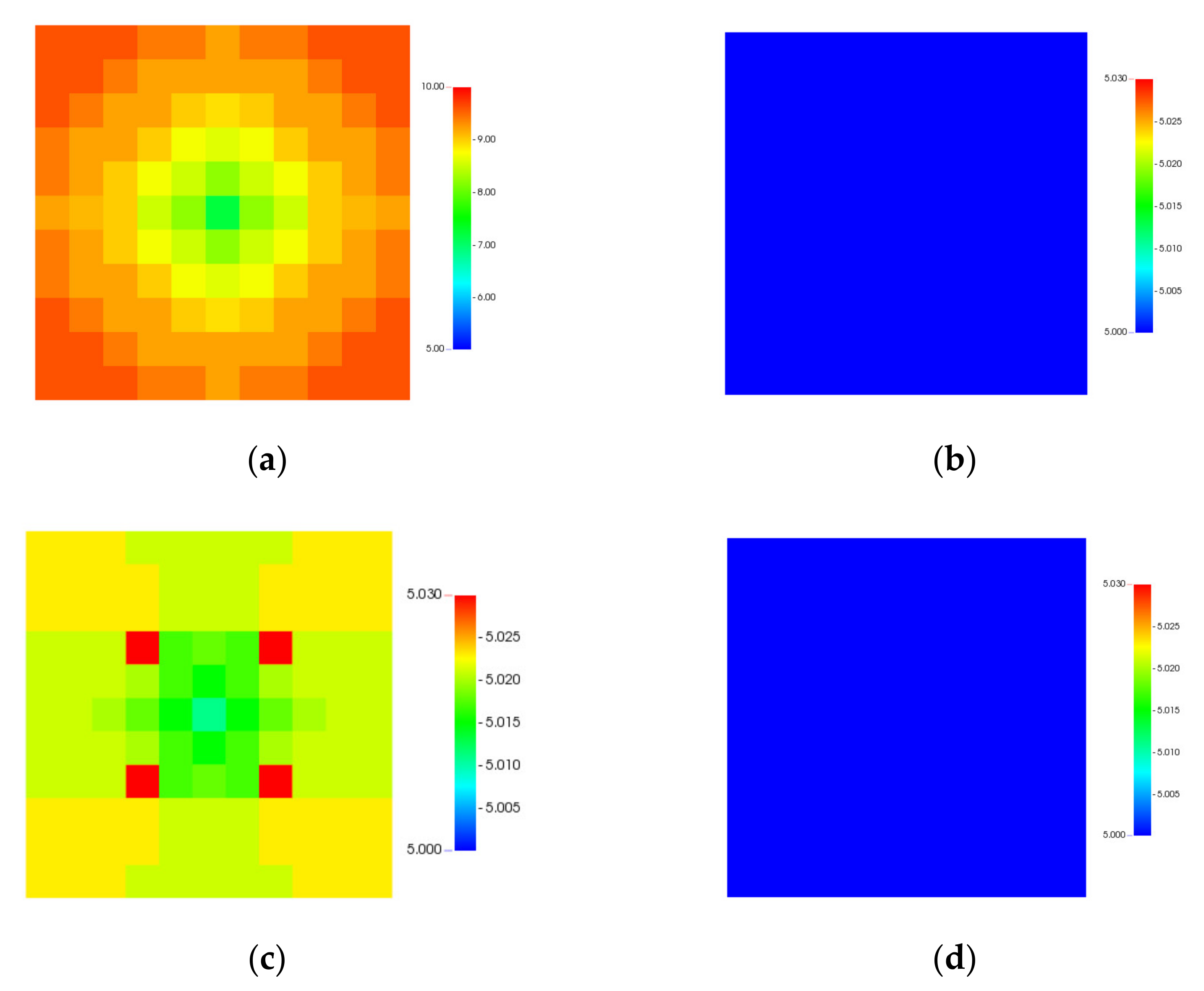
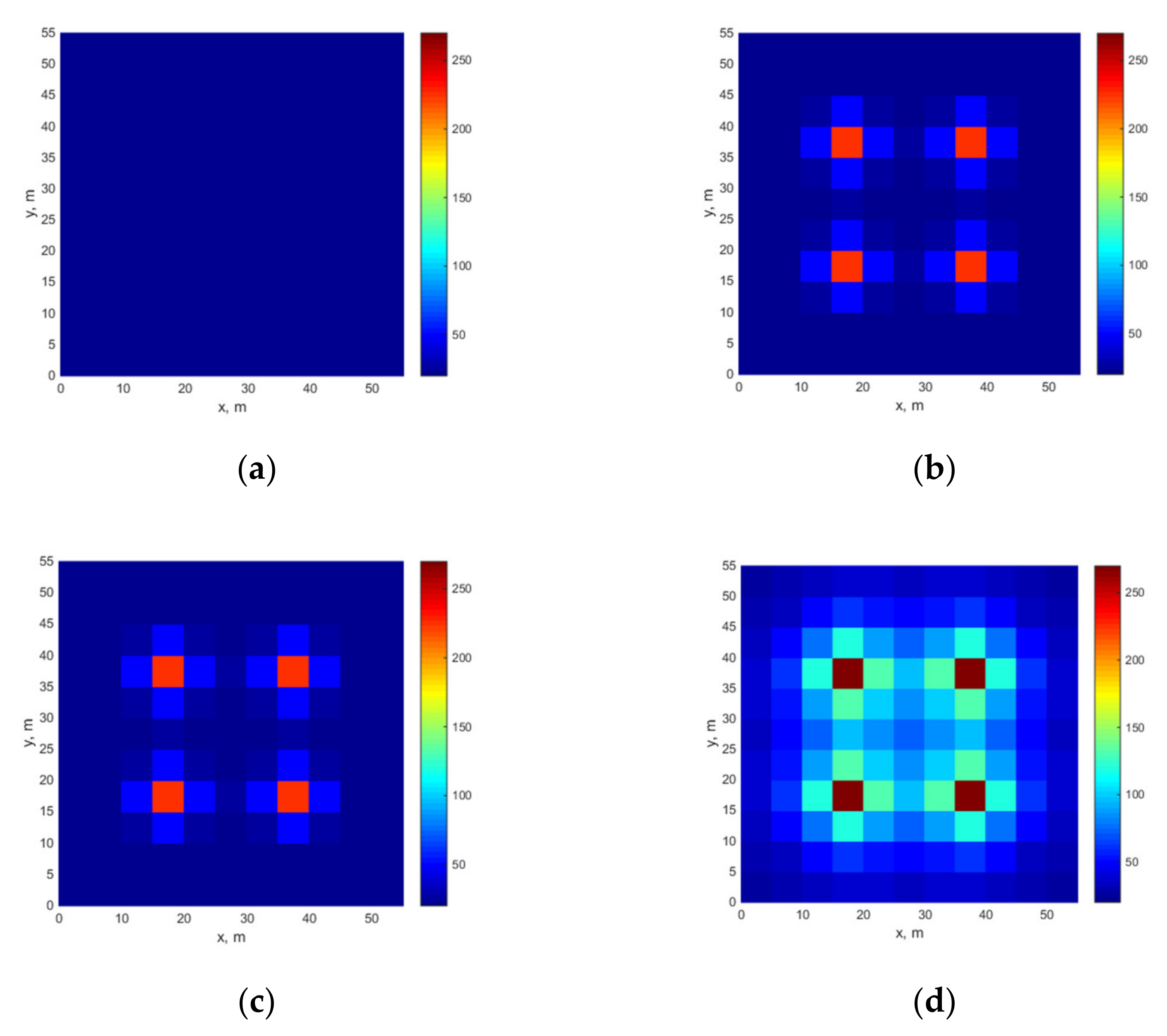
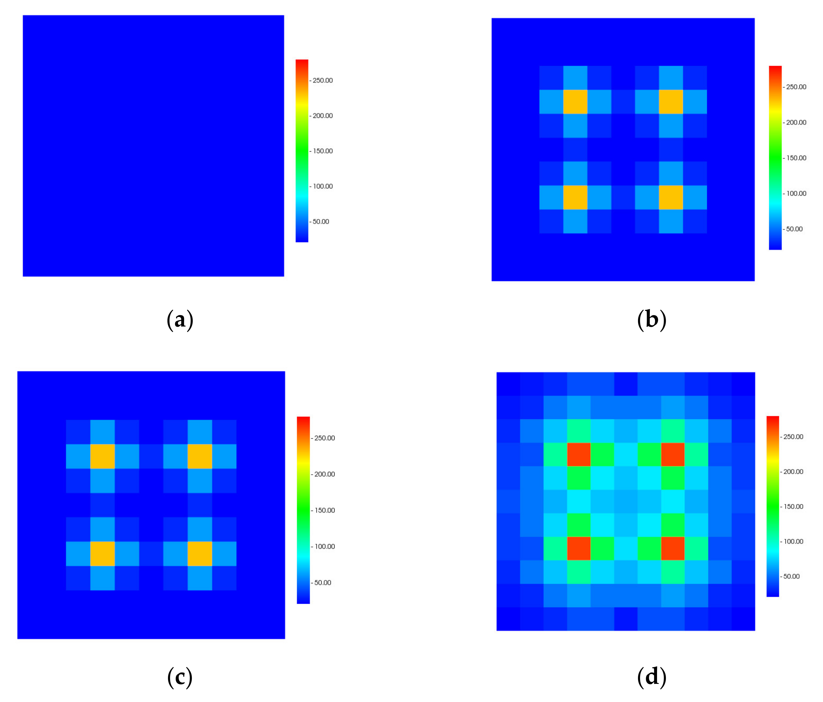
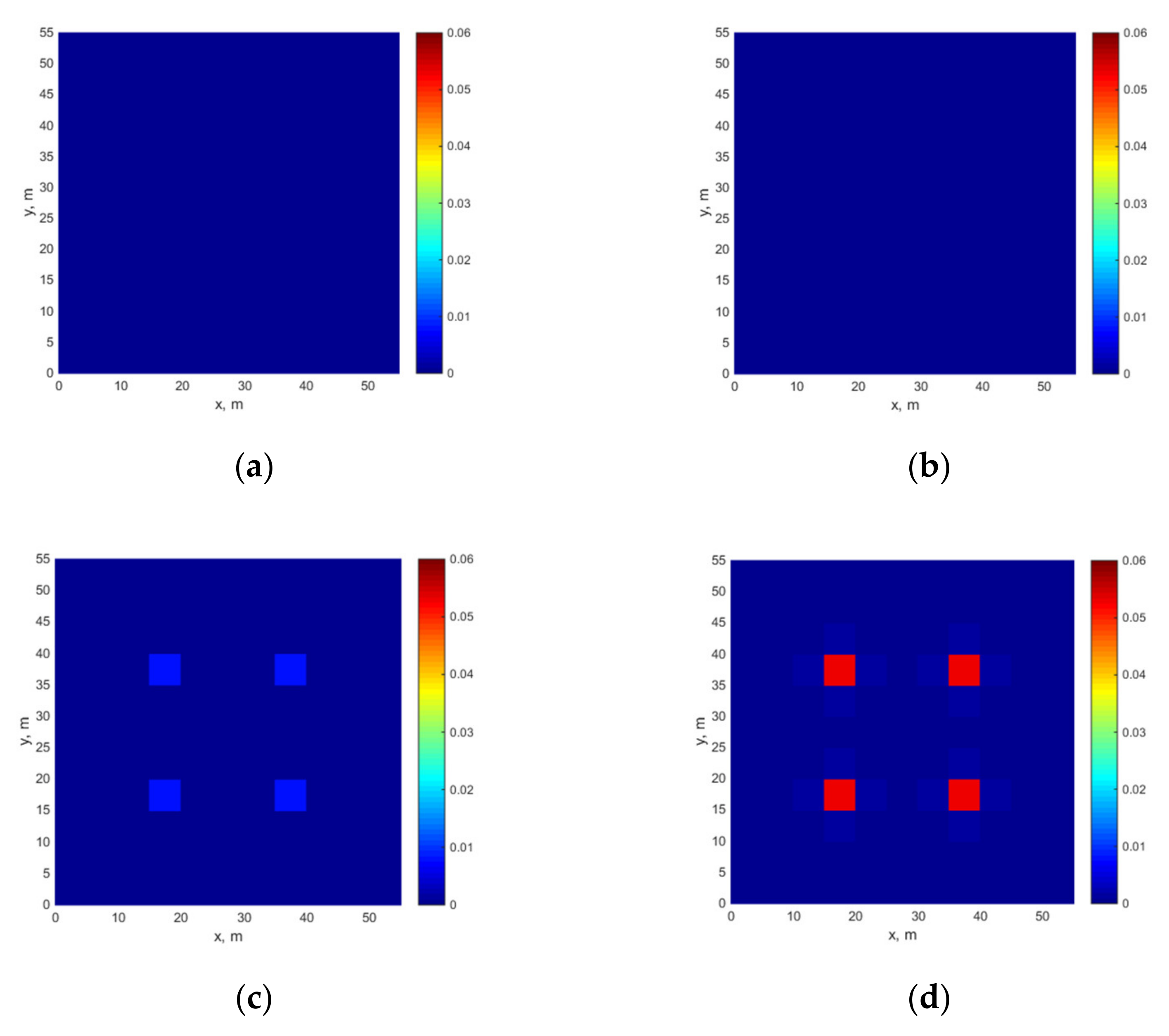
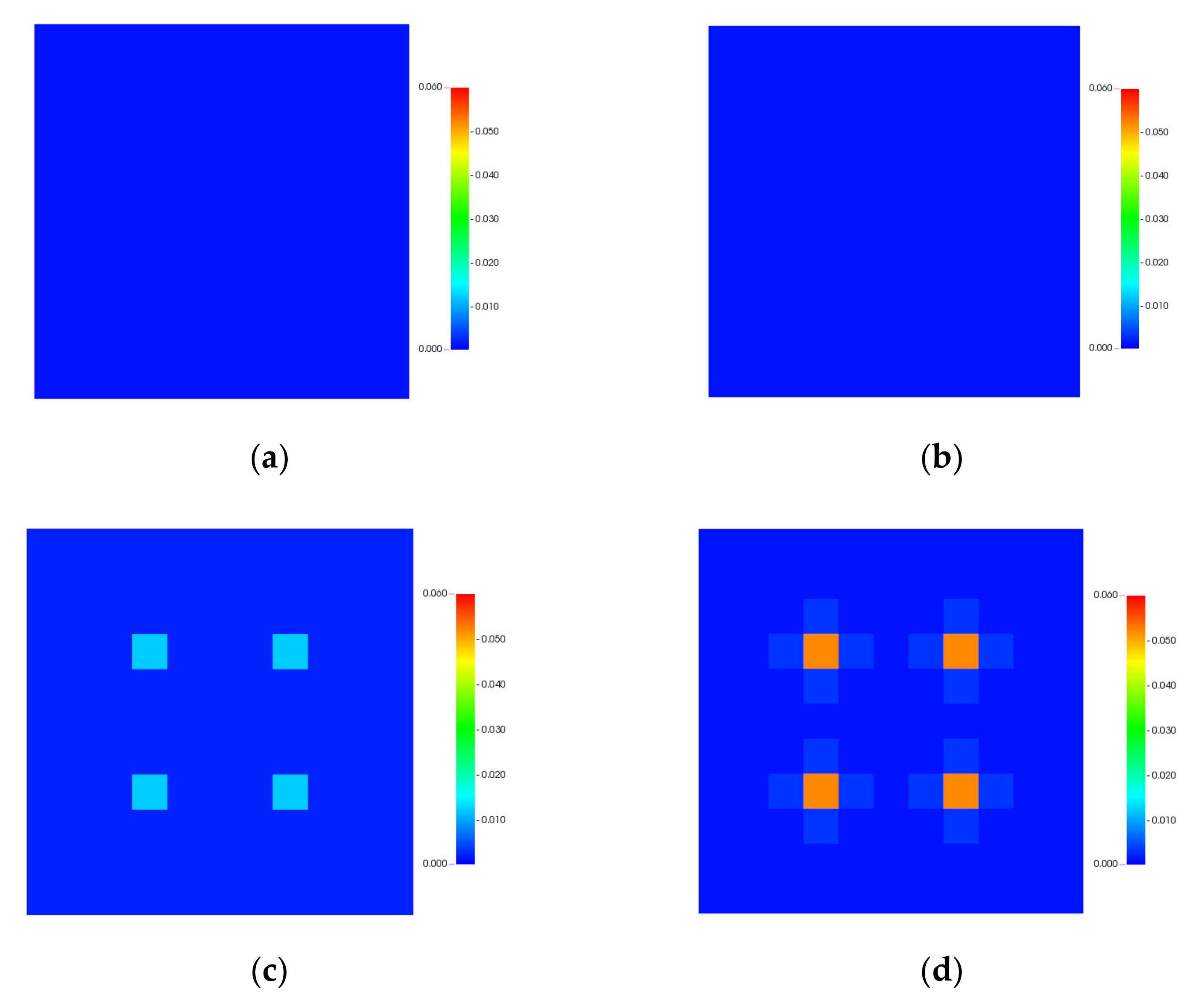
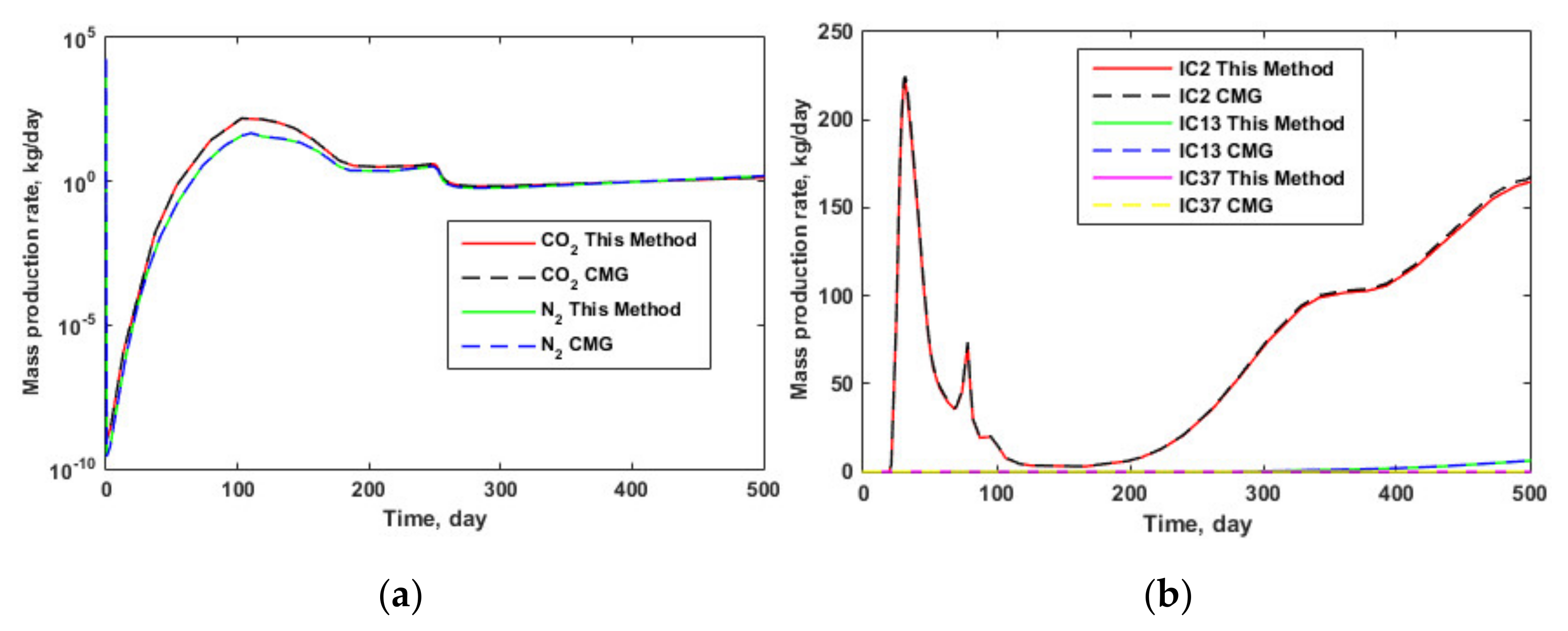
As shown in Figure 2, this example is a two-dimensional reservoir model, and the grid size is 5 m × 5 m, the grid division is 11 × 11. The reservoir thickness is 5 m and the initial pressure is 10 MPa. The reservoir boundary is closed both in terms of the mass and heat transfer. The heat injection grids are (4,4), (4,8), (8,4), (8,4), the constant temperature of the heating device is 370 °C, the grid where the production well is located is (6,6), and the production pressure is 5 MPa. The chemical reaction in this example is shown in Equation (37), and the corresponding chemical reaction coefficient is shown in Table 1, The enthalpy of each component is calculated according to the fifth degree polynomial function about temperature [6]. Other basic fluids, thermal, and reservoir parameters are shown in Table 2. The coefficients of the polynomial function can be seen in Fan et al. [6]. Figure 3 and Figure 4, respectively, show pressure profiles at 0.001, 10, 30, and 200 days calculated by this method and CMG. Figure 5 and Figure 6, respectively, show the oil saturation profiles at 0.001, 10, 30, and 200 days calculated by this method and CMG. Figure 7 and Figure 8, respectively, compare the oil saturation profiles at different times calculated by this method. Figure 9 compares the production rates of components for 500 days calculated by this method and CMG, respectively. Comparisons of calculation results from this method and CMG illustrate that this method can obtain high-accuracy results.
In addition, it can also be seen that, at the initial stage of production, the pyrolysis reaction rate of solid kerogen-producing liquid and gaseous organic matter is very low, resulting in the pressure drop of depleted exploitation of the saturated inorganic CO2 and N2 in the reservoir pores, shown in Figure 3a at the beginning of production; and then Figure 3b shows the depleted pressure wave diffuses to the boundary. The pressure of the whole reservoir calculation domain is very close to the bottom hole flow pressure (BHP). Then, with the increase of the surrounding temperature of the heating device shown in Figure 5, the pyrolysis reaction rate of solid kerogen increases. The IC2, IC13, IC37, and CO2 produced by pyrolysis increase the pressure near the heating device, that is, the pressure distribution shown in Figure 3c. Finally, as shown in Figure 3d, the organic and inorganic substances produced by pyrolysis reaction are recovered, and the pressure of the whole reservoir calculation domain is reduced to close to the BHP again. Besides, with the increase of pyrolysis reaction rate of oil shale, the rate of carbon dioxide produced by pyrolysis is also faster, resulting in the output of CO2 in the later stage of production being higher than that of N2.
3.2. A 3D Example with a Steam Injection Well
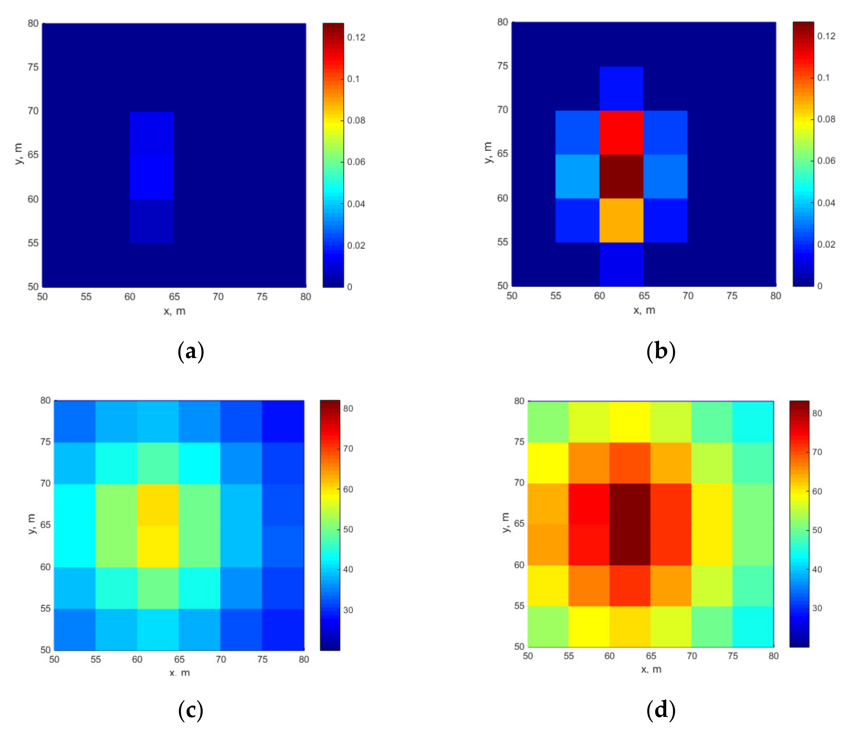
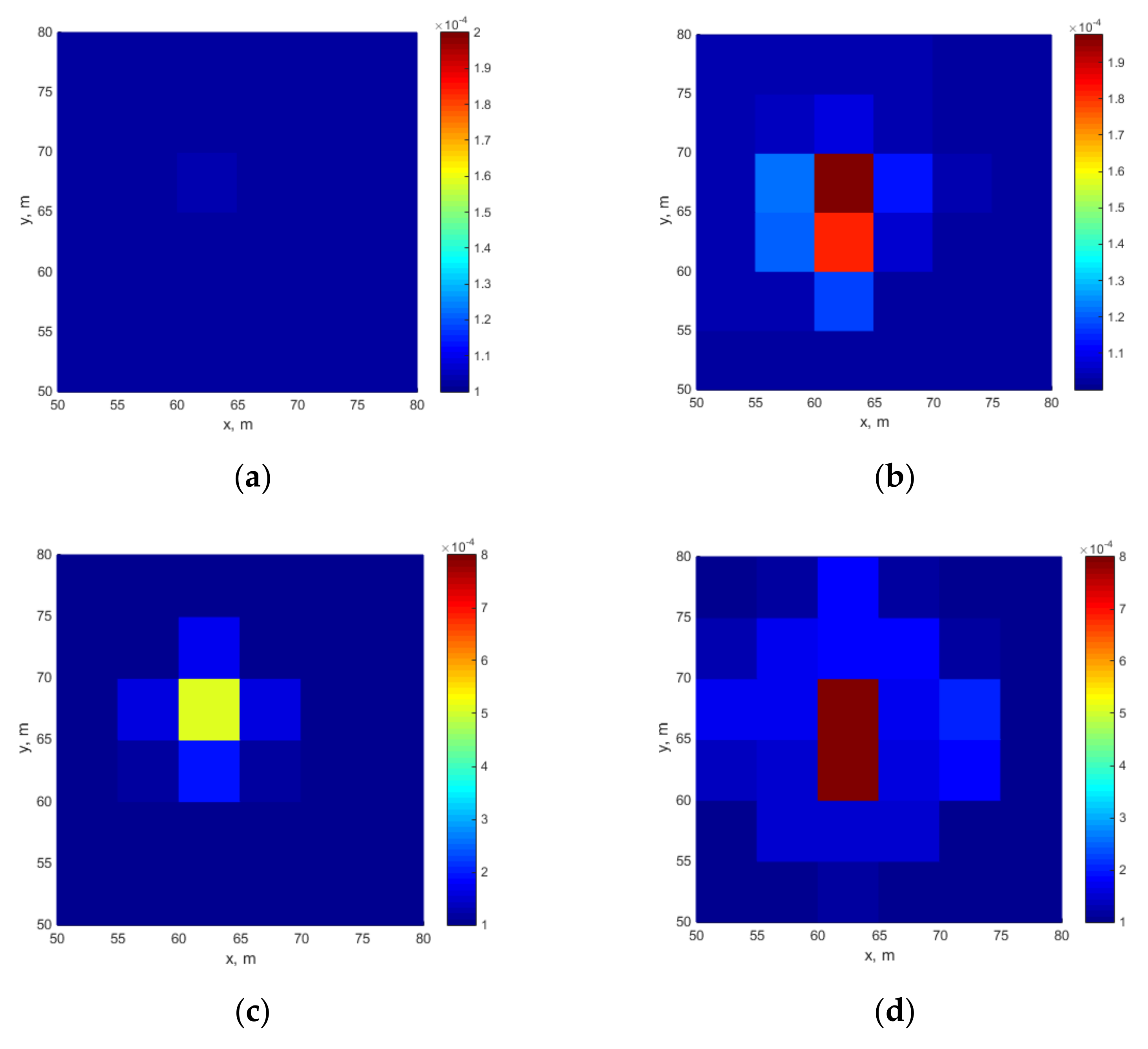
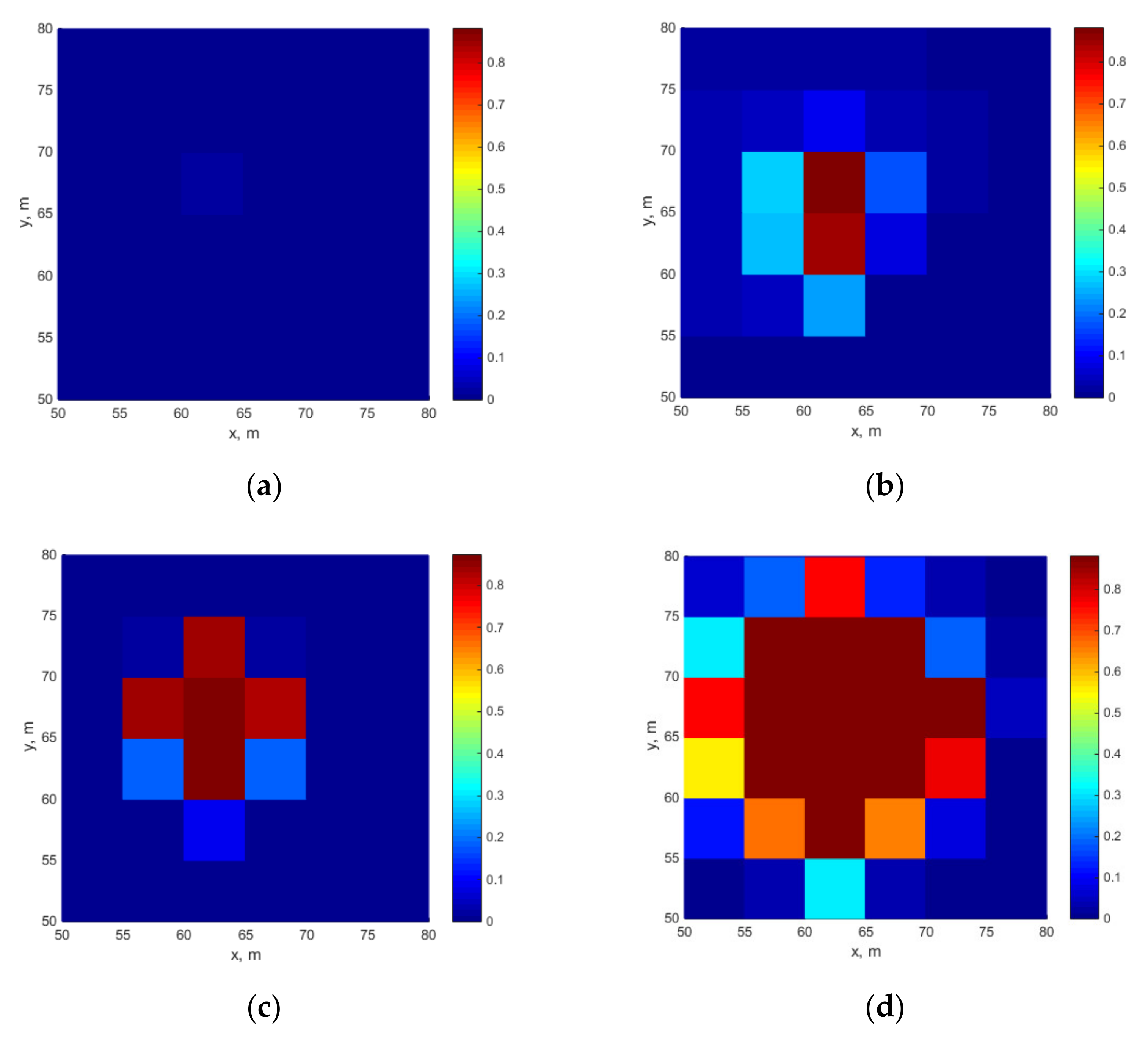
As shown in Figure 10, this example is an oil shale reservoir with a size of 30 m × 30 m * 18 m. It is divided into two layers longitudinally, and a circle of heat transfer layer is added outside the boundary. The initial conditions of this reservoir model are listed in Table 3, and related physical and thermal parameters are the same as those in Table 1. The reservoir boundary is closed but thermally open, and the pyrolysis reaction of oil shale is the same as that in Equation (37). There is a fractured vertical well for steam injection, the injection rate is 25 tons/day, the steam temperature is 480 °C, and a production well is controlled by a fixed BHP of 5 MPa. The pressure distribution in Figure 10c can also reflect the well locations, and the simulation time lasts for 800 days, Figure 11 shows the calculated temperature and water saturation at different times. It can be seen that the water saturation distribution is positively correlated with the temperature distribution, and the injected steam is effectively heating the formation. Figure 12 and Figure 13 also show the calculated oil saturation and IC2 light component in the gas phase, respectively. Figure 12 shows that the oil saturation increases with the continuous heat injection, and the corresponding concentration of IC2 component in the gas phase in Figure 13 also increases, indicating that a large number of IC2 light components are produced by oil shale pyrolysis, and the profiles of the concentration of IC2 component in the gas phase is basically consistent with the profiles of oil saturation, which represents the distribution of the intensity of the oil shale pyrolysis reaction. Because the fracture only penetrates the lower layer, the lower layer is heated more, the reaction is stronger, and the difference between layers is obvious.
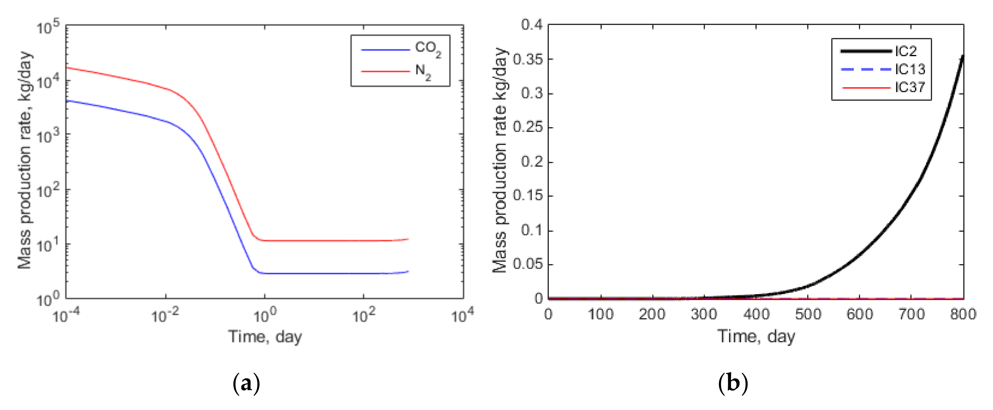
Figure 14 shows the calculated production rates of the components for 800 days. The production curves of inorganic and organic components of the well can also be obtained. It can be seen that, during early production, the production rate of saturated N2 and CO2 declines sharply. In less than a day, almost all the inorganic gases in the formation have been extracted. Moreover, since the chemical reaction coefficient of the light component IC2 in the pyrolysis reaction is the largest, and the proportion of the light component IC2 in the gas phase at phase equilibrium is much higher than that of the heavy components IC13 and IC37, the light component IC2 will be recovered first with the increase of the chemical reaction speed caused by the continuous temperature increase with steam injection. The output of the organic components is low in this small-scale toy model, so we can continue to simulate and calculate the production performance for a longer time, or improve the steam injection rate to produce organic components faster.
4. Conclusions and Future Work
This paper presents an effective numerical simulation method for oil-shale in situ production. Firstly, the finite volume discrete scheme of mass and heat transfer equation for oil shale in situ production is derived, and the hydraulic fracture of the steam injection well is treated by using the embedded discrete fracture model. Then, a non-linear solver which does not need to judge phase transformation and can give unified constraints on phase saturation and component concentration is given, Thus, the mass and heat transfer equation of oil shale can be solved more smoothly. A numerical example compared with CMG shows that the method based on the smooth non-linear solver can achieve accurate results. Through a numerical example with a fractured vertical well and open thermal boundary conditions, it is verified that this method can effectively deal with the actual situation of steam injection-assisted oil shale production which is difficult to deal with by the previous methods.
There are several limitations in this paper: (1) although the presented smooth nonlinear solver ensures that the equation form of each grid is always the same in the process of simulation calculation, additional constraint equations shown in Equation (20) are added, and the more components, the more additional equations are added, significantly increasing the computational cost. Therefore, it will be valuable in future work to strictly analyze and compare the calculation efficiency and accuracy between the presented non-linear solver and the widely used non-linear solver of the thermal composition model for oil-shale in situ recovery based on natural formulations. (2) In the processing method of the thermally open condition given in this paper, if the grid size added outside the boundary of the computing domain is too large, the approximation accuracy of the thermally open condition will be reduced. If the grid size is small, more grids need to be added, which will reduce the computing efficiency. How to determine the optimal strategy of adding grids or develop a better thermally open condition processing method will be valuable to ascertain in future work. (3) In this paper, only some small-scale conceptual examples are calculated and tested. The application of this method in the actual large-scale oil-shale development can be further studied. (4) The application of the presented smooth non-linear solver in the steam-flooding reservoir and the thermochemical-flooding reservoir can be further explored.
Author Contributions
Conceptualization, X.R. and X.C.; methodology, X.R. and X.C.; software, X.R. and X.C.; validation, X.R. and X.C. and Y.X.; formal analysis, X.R. and X.C.; investigation, X.R. and X.C.; resources, X.R. and X.C.; data curation, X.R. and Y.X.; writing—original draft preparation, X.R.; writing—review and editing, X.R., X.C. and Y.L.; visualization, X.R. and Y.X.; supervision, X.R. and X.C.; project administration, X.C. and X.R.; funding acquisition, X.C. and X.R. All authors have read and agreed to the published version of the manuscript.
Funding
Authors thank the supports from the National Key Research and Development Program of China (Grant Nos. 2019YFA0705501) and the open fund of the State Center for Research and Development of Oil Shale Exploitation (33550000-21-ZC0611-0008), and the National Natural Science Foundation of China (Grant No. 52104017).
Institutional Review Board Statement
Not applicable.
Informed Consent Statement
Not applicable.
Data Availability Statement
The data presented in this study are available on request from the corresponding author. The data are not publicly available due to the data are related with development of the simulator.
Acknowledgments
Authors thank the constructive suggestions from the reviewers.
Conflicts of Interest
The authors declare no conflict of interest.
Nomenclature
| ρ | density |
| u | Seepage velocity |
| X | the concentration of a component in a phase |
| ν′ | stoichiometric coefficients as product |
| ν | stoichiometric coefficients as a reactant |
| r | the rate of a reaction |
| q | the source or sink term |
| t | time |
| ϕ | porosity |
| S | saturation |
| k | permeability |
| kr | relative permeability |
| μ | viscosity |
| p | pressure |
| γ | gravity |
| D | reservoir depth |
| C | concentration |
| λ | mobility |
| T | temperature |
| H | enthalpy |
| qH | heat source term |
| U | the internal energy |
| K | reaction rate constant |
| E | activation energy |
| R | Boltzmann constant |
| T | gas temperature |
| Cl | the kerogen concentration in the solid phase |
| WI | well index for mass transfer |
| pwf | bottom hole pressure |
| re | effective radius in Peaceman formula for well index calculation |
| rW | well radius |
| HI | well index for heat transfer |
| G | geometric factor |
| T′ | the mass transmissibility between two cells |
| V | the grid volume |
| Q | the mass production or injection rate of a well |
| QH | the heat production or injection rate of a well |
| g | Gravitational acceleration |
| B | volume factor |
| Af | area of a fracture cell |
| 〈d〉 | the average distance from points in a matrix grid to its containing fracture cell |
| unit normal vector | |
| Ω | the domain of a matrix cell |
| Sor | oil residual saturation |
| t + Δt | the time t + Δt |
| t | the time t |
| W | terms related to the well |
| j | the j-th phase |
| i | the i-th component |
| h | the h-th grid |
| k | the k-th grid |
| hk | terms between the h-th and the k-th grid |
| m | index of a matrix grid |
| f | index of a fracture grid |
| kero | kerogen |
| C | coke |
| o | oil phase |
| w | water phase |
| r | rock |
| l | the l-th reaction |
| sc | standard condition |
References
- Burnham, A.K.; Braun, R.L. General kinetic model of oil shale pyrolysis. In Situ 1985, 9, 1–23. [Google Scholar]
- Braun, R.L.; Burnham, A.K. Mathematical model of oil generation, degradation, and expulsion. Energy Fuels 1990, 4, 132–146. [Google Scholar] [CrossRef]
- Braun, R.L.; Burnham, A.K. Chemical Reaction Model for Oil and Gas Generation from Type 1 and Type 2 Kerogen; Lawrence Livermore National Laboratory: Livermore, CA, USA, 1993. [Google Scholar]
- Taheri-Shakib, J.; Kantzas, A. A comprehensive review of microwave application on the oil shale: Prospects for shale oil production. Fuel 2021, 305, 121519. [Google Scholar] [CrossRef]
- Vinegar, H.; Nguyen, S. Method and Apparatus for Generating and/or Hydrotreating Hydrocarbon Formation Fluids. U.S. Patent Application No. 14/412,698, 19 September 2015. [Google Scholar]
- Shen, C. Reservoir simulation study of an in-situ conversion pilot of Green-River oil shale. In Proceedings of the SPE Rocky Mountain Petroleum Technology Conference SPE-142-MS, Denver, CO, USA, 14–16 April 2009. [Google Scholar]
- Fan, Y.; Durlofsky, L.; Tchelepi, H.A. Numerical simulation of the in-situ upgrading of oil shale. SPE J. 2010, 15, 368–381. [Google Scholar] [CrossRef]
- Kang, Z.; Zhao, Y.; Yang, D.; Tian, L.; Li, X. A pilot investigation of pyrolysis from oil and gas extraction from oil shale by in-situ superheated steam injection. J. Pet. Sci. Eng. 2020, 186, 106785. [Google Scholar] [CrossRef]
- Pei, S.; Wang, Y.; Zhang, L.; Huang, L.; Cui, G.; Zhang, P.; Ren, S. An innovative nitrogen injection assisted in-situ conversion process for oil shale recovery: Mechanism and reservoir simulation study. J. Pet. Sci. Eng. 2018, 171, 507–515. [Google Scholar] [CrossRef]
- Wang, G.; Liu, S.; Yang, D.; Fu, M. Numerical study on the in-situ pyrolysis process of steeply dipping oil shale deposits by injecting superheated water steam: A case study on Jimsar oil shale in Xinjiang, China. Energy 2022, 239, 122182. [Google Scholar] [CrossRef]
- Taheri Shakib, J.; Akhgarian, E.; Ghaderi, A. The effect of hydraulic fracture characteristics on production rate in thermal EOR methods. Fuel 2015, 141, 226–235. [Google Scholar] [CrossRef]
- Rao, X.; Cheng, L.; Cao, R.; Jia, P.; Liu, H.; Du, X. A modified projection-based embedded discrete fracture model (pEDFM) for practical and accurate numerical simulation of fractured reservoir. J. Pet. Sci. Eng. 2020, 187, 106852. [Google Scholar] [CrossRef]
- Rao, X.; Xin, L.; He, Y.; Fang, X.; Gong, R.; Wang, F.; Zhao, H.; Shi, J.; Xu, Y.; Dai, W. Numerical simulation of two-phase heat and mass transfer in fractured reservoirs based on projection-based embedded discrete fracture model (pEDFM). J. Pet. Sci. Eng. 2022, 208, 109323. [Google Scholar] [CrossRef]
- Rao, X. A Numerical Modelling Method of Fractured Reservoirs with Embedded Meshes and Topological Fracture Projection Configurations. Comput. Model. Eng. Sci. 2022. [Google Scholar] [CrossRef]
- Ghaderi, A.; Taheri-Shakib, J.; Nik, S.A.M. The distinct element method (DEM) and the extended finite element method (XFEM) application for analysis of interaction between hydraulic and natural fractures. J. Pet. Sci. Eng. 2018, 171, 422–430. [Google Scholar] [CrossRef]
- Li, H.; Vink, J.C.; Alpak, F.O. A Dual-Grid Method for the Upscaling of Solid-Based Thermal Reactive Flow, With Application to the In-Situ Conversion Process. SPE J. 2016, 21, 2097–2111. [Google Scholar] [CrossRef]
- Li, H.; Durlofsky, L.J. Upscaling for Compositional Reservoir Simulation. SPE J. 2016, 21, 873–887. [Google Scholar] [CrossRef]
- Zheng, H.; Shi, W.; Ding, D.; Zhang, C. Numerical simulation of in situ combustion of oil shale. Geofluids 2017, 2017, 3028974. [Google Scholar] [CrossRef] [Green Version]
- Kelkarl, S.; Pawar, R.; Hoda, N. Numerical Simulation of Coupled Thermal-Hydrological-Mechanical Chemical Processes during In Situ Conversion and Production of Oil Shale. In Proceedings of the 31st Oil Shale Symposium, Golden, CO, USA, 17–19 October 2011. [Google Scholar]
- Li, X.; He, Y.; Huo, M.; Yang, Z.; Wang, H.; Song, R. Simulation of coupled thermal-hydro-mechanical processes in fracture propagation of carbon dioxide fracturing in oil shale reservoirs. Energy Sources Part A Recovery Util. Environ. Eff. 2019, 1–20. [Google Scholar] [CrossRef]
- Ghaderi, A.; Taheri-Shakib, J.; Sharifnik, M.A. The effect of natural fracture on the fluid leak-off in hydraulic fracturing treatment. Petroleum 2019, 5, 85–89. [Google Scholar] [CrossRef]
- Boak, J.; Kleinberg, R. Shale Gas, Tight Oil, Shale Oil and Hydraulic Fracturing. In Future Energy; Elsevier: Amsterdam, The Netherlands, 2020; pp. 67–95. [Google Scholar] [CrossRef]
- Taheri-Shakib, J.; Ghaderi, A.; Kanani, V.; Rajabi-Kochi, M.; Hosseini, S.A. Numerical analysis of production rate based on interaction between induced and natural fractures in porous media. J. Pet. Sci. Eng. 2018, 165, 243–252. [Google Scholar] [CrossRef]
- Taheri-Shakib, J.; Ghaderi, A.; Sharif Nik, M.A. Numerical study of influence of hydraulic fracturing on fluid flow in natural fractures. Petroleum 2018, 5, 321–328. [Google Scholar] [CrossRef]
Figure 1.
Sketches of boundary treatment. (a) Permeability profile; (b) pressure profile.

Figure 2.
Sketch of 2D reservoir model in this example. (a) this model; (b) Computer Modeling Group (CMG) model.
Figure 2.
Sketch of 2D reservoir model in this example. (a) this model; (b) Computer Modeling Group (CMG) model.

Figure 3.
Reservoir pressure profiles calculated by this method.

Figure 4.
Reservoir pressure profiles calculated by CMG. (a) The 0.001th day; (b) the 10th day; (c) the 30th day; (d) the 200th day.
Figure 4.
Reservoir pressure profiles calculated by CMG. (a) The 0.001th day; (b) the 10th day; (c) the 30th day; (d) the 200th day.

Figure 5.
Reservoir temperature profiles calculated by this method. (a) The 0.001th day; (b) the 10th day; (c) the 30th day; (d) the 200th day.
Figure 5.
Reservoir temperature profiles calculated by this method. (a) The 0.001th day; (b) the 10th day; (c) the 30th day; (d) the 200th day.

Figure 6.
Reservoir temperature profiles calculated by CMG. (a) The 0.001th day; (b) the 10th day; (c) the 30th day; (d) the 200th day.
Figure 6.
Reservoir temperature profiles calculated by CMG. (a) The 0.001th day; (b) the 10th day; (c) the 30th day; (d) the 200th day.

Figure 7.
Reservoir oil saturation profiles calculated by this method. (a) The 0.001th day; (b) the 10th day; (c) the 30th day; (d) the 200th day.
Figure 7.
Reservoir oil saturation profiles calculated by this method. (a) The 0.001th day; (b) the 10th day; (c) the 30th day; (d) the 200th day.

Figure 8.
Reservoir oil saturation profiles calculated by CMG. (a) The 0.001th day; (b) the 10th day; (c) the 30th day; (d) the 200th day.
Figure 8.
Reservoir oil saturation profiles calculated by CMG. (a) The 0.001th day; (b) the 10th day; (c) the 30th day; (d) the 200th day.

Figure 9.
Production curves of this reservoir model. (a) Inorganic component; (b) organic component.
Figure 9.
Production curves of this reservoir model. (a) Inorganic component; (b) organic component.

Figure 10.
Geometric view of the reservoir model. (a) The 3D view; (b) 2D view; (c) a pressure profile.
Figure 10.
Geometric view of the reservoir model. (a) The 3D view; (b) 2D view; (c) a pressure profile.

Figure 11.
Profiles of the calculated water saturation and temperature: (a) 400 days, water saturation; (b) 800 days, water saturation; (c) 400 days, temperature; (d) 800 days, temperature.
Figure 11.
Profiles of the calculated water saturation and temperature: (a) 400 days, water saturation; (b) 800 days, water saturation; (c) 400 days, temperature; (d) 800 days, temperature.

Figure 12.
Profiles of the calculated oil saturation: (a) 400 days, upper layer; (b) 800 days, upper layer; (c) 400 days, lower layer; (d) 800 days, lower layer.
Figure 12.
Profiles of the calculated oil saturation: (a) 400 days, upper layer; (b) 800 days, upper layer; (c) 400 days, lower layer; (d) 800 days, lower layer.

Figure 13.
Profiles of the concentration of IC2 light component in gas phase: (a) 400 days, upper layer; (b) 800 days, upper layer; (c) 400 days, lower layer; (d) 800 days, lower layer.
Figure 13.
Profiles of the concentration of IC2 light component in gas phase: (a) 400 days, upper layer; (b) 800 days, upper layer; (c) 400 days, lower layer; (d) 800 days, lower layer.

Figure 14.
Production curves of inorganic and organic components of production wells calculated. (a) Inorganic component; (b) organic component.
Figure 14.
Production curves of inorganic and organic components of production wells calculated. (a) Inorganic component; (b) organic component.


Table 1.
Chemical reaction coefficient of kerogen pyrolysis.
| Chemical Reaction Coefficient | Frequency Factor | The Activation Energy (KJ/mol) | |||||
|---|---|---|---|---|---|---|---|
| kerogen | IC2 | IC13 | IC37 | CO2 | |||
| reaction | 1 | 0 | 0 | 0 | 0 | 3.74 × 10¹² | 161.600 |
| production | 0 | 0.04475 | 0.0178 | 0.0096 | 0.00541 | ||
Table 2.
Value physical properties.
| Property | Value | Property | Value |
|---|---|---|---|
| Initial water saturation, fraction | 0 | Rock thermal conductivity, J/(m·s·K) | 3 |
| Initial gas saturation, fraction | 0.1499 | Solid-phase thermal conductivity, J/(m·s·K) | 3 |
| Initial oil saturation, fraction | 0.0001 | Oil phase thermal conductivity, J/(m·s·K) | 0.6 |
| Initial solid saturation, fraction | 0.8500 | Water phase thermal conductivity, J/(m·s·K) | 0.2 |
| Kerogen concentration in a solid phase, fraction | 1 | Gas-phase thermal conductivity, J/(m·s·K) | 0.1 |
| Initial reservoir temperature, °C | 20 °C | Initial oil viscosity, mPa·s | 50 |
| Initial porosity, fraction | 0.3 | Water viscosity, mPa·s | 0.6 |
| Permeability, mD | 1 | Gas viscosity, mPa·s | 0.01 |
| Rock density, kg/m³ | 2700 | Rock compressibility, MPa−1 | 1.07 × 10⁻⁴ |
| Solid density, kg/m³ | 2000 | Solid-phase compressibility, MPa−1 | 1.07 × 10⁻⁴ |
| Oil density, kg/m³ | 877 | Oil phase compressibility, MPa−1 | 3.02 × 10⁻³ |
| Gas density, kg/m³ | 26 | Water phase compressibility, MPa−1 | 5 × 10⁻⁴ |
| Water density, kg/m³ | 1000 | Gas phase compressibility, MPa−1 | 5 × 10⁻² |
Table 3.
Initial conditions.
| Initial Conditions | Values |
|---|---|
| Pressure, MPa | 10 |
| Water saturation, fraction | 0 |
| Gas saturation, fraction | 0.15 |
| Temperature, fraction | 20 |
| Solid-phase saturation, fraction | 0.85 |
| N2 concentration in gas phase, fraction | 0.2 |
| CO2 concentration in the gas phase, fraction | 0.8 |
| Kerogen concentration in the solid phase, fraction | 1 |
Publisher’s Note: MDPI stays neutral with regard to jurisdictional claims in published maps and institutional affiliations. |
© 2022 by the authors. Licensee MDPI, Basel, Switzerland. This article is an open access article distributed under the terms and conditions of the Creative Commons Attribution (CC BY) license (https://creativecommons.org/licenses/by/4.0/).
Share and Cite
MDPI and ACS Style
Chen, X.; Rao, X.; Xu, Y.; Liu, Y. An Effective Numerical Simulation Method for Steam Injection Assisted In Situ Recovery of Oil Shale. Energies 2022, 15, 776. https://0-doi-org.brum.beds.ac.uk/10.3390/en15030776
AMA Style
Chen X, Rao X, Xu Y, Liu Y. An Effective Numerical Simulation Method for Steam Injection Assisted In Situ Recovery of Oil Shale. Energies. 2022; 15(3):776. https://0-doi-org.brum.beds.ac.uk/10.3390/en15030776
Chicago/Turabian StyleChen, Xudong, Xiang Rao, Yunfeng Xu, and Yina Liu. 2022. "An Effective Numerical Simulation Method for Steam Injection Assisted In Situ Recovery of Oil Shale" Energies 15, no. 3: 776. https://0-doi-org.brum.beds.ac.uk/10.3390/en15030776
Note that from the first issue of 2016, this journal uses article numbers instead of page numbers. See further details here.