
Probabilistic Optimization Techniques in Smart Power System


1
Department of Electrical and Computer Engineering, Wah Campus, COMSATS University, Wah 47040, Pakistan
2
Faculty of Electrical and Computer Engineering, University of Engineering and Technology Peshawar, Peshawar 25000, Pakistan
3
Faculty of Information Technology, Engineering and Economics, Oestfold University College, 1757 Halden, Norway
*
Authors to whom correspondence should be addressed.
Energies 2022, 15(3), 825; https://0-doi-org.brum.beds.ac.uk/10.3390/en15030825
Submission received: 20 November 2021
/
Revised: 17 January 2022
/
Accepted: 19 January 2022
/
Published: 24 January 2022
(This article belongs to the Special Issue Power System Dynamics and Renewable Energy Integration)
Abstract
:Uncertainties are the most significant challenges in the smart power system, necessitating the use of precise techniques to deal with them properly. Such problems could be effectively solved using a probabilistic optimization strategy. It is further divided into stochastic, robust, distributionally robust, and chance-constrained optimizations. The topics of probabilistic optimization in smart power systems are covered in this review paper. In order to account for uncertainty in optimization processes, stochastic optimization is essential. Robust optimization is the most advanced approach to optimize a system under uncertainty, in which a deterministic, set-based uncertainty model is used instead of a stochastic one. The computational complexity of stochastic programming and the conservativeness of robust optimization are both reduced by distributionally robust optimization.Chance constrained algorithms help in solving the constraints optimization problems, where finite probability get violated. This review paper discusses microgrid and home energy management, demand-side management, unit commitment, microgrid integration, and economic dispatch as examples of applications of these techniques in smart power systems. Probabilistic mathematical models of different scenarios, for which deterministic approaches have been used in the literature, are also presented. Future research directions in a variety of smart power system domains are also presented.
1. Introduction
Energy demand is expanding in lockstep with global population expansion, resulting in a supply-demand mismatch. Increased generation capacity or load reduction can help close the demand-supply imbalance. Increased generation capacity is possible through the use of fossil fuels, which are costly and pollutant [1]. Enhancing generation capacity through the integration of renewable energy resources into the smart power system is beneficial. Load curtailment creates user displeasure, which can be mitigated by implementing appropriate demand-side policies. The integration of renewable energy supplies and variable load introduces a number of risks into the smart power system that must be handled. This article discusses uncertainty in a variety of sectors related to smart power systems. This is explained in greater detail below.
1.1. Smart Power System
Conventional grid electrical power is sent unidirectionally from a central power station to remote users. In 2000, a smart power system concept was established with the primary goal of integrating two-way communication into the infrastructure of a standard grid system. From the generating station to the consumers, a smart power system integrates communication and information technology [2,3]. Consumers receive safe, robust, and high-quality power from a smart power system [4,5,6]. To transform a traditional grid into a smart power system, a scalable yet robust communication architecture is necessary [7]. In an electrical power system, the grid is composed of multiple energy generating, transmission, distribution, and control elements. The smart power system intelligently organizes and connects the traditional grid’s elements previously stated [8,9,10].
In a smart power system, generating stations serve as the primary unit. Energy from renewable sources is required for new power plants since fossil fuels are becoming depleted and have other negative effects on the environment. Solar and wind energy have unpredictable output power since they are weather-dependent; as a result, the operation of smart power systems is affected as mentioned in [11,12,13]. Electrical power supply relies heavily on transmission systems because generating units are located distant from the end-users of the electricity. Climate change has a direct impact on the transmission system, resulting in issues such as wind and temperature stress. These uncertainties have a significant impact on the transmission system’s performance and life expectancy [14].
Intelligent distribution systems are a critical component of a smart power system. It is composed of a variety of sensors and smart sensing mechanisms, as well as a sensor network that includes smart metres, distribution transformer management, and monitoring. Due to the usage of these sensors, a smart grid can monitor the health of the grid in real time and utilize the data to operate the grid in a reliable, secure, and stable manner, while also reducing costs and increasing energy efficiency. Sensors and actuators play a critical role in the energy management of smart power systems in this context [15,16]. Employing sensors for real-time monitoring helps to deal with the power management of distributed energy resources, such as distributed generators (DGs) [17] and electric vehicles [18], as well as to improve the smart grid’s reliability as it makes the integration of renewable energy resources much more convenient and improves both the efficiency and reliability of smart power system [19,20]. Due to the integration of distributed generation, the smart distribution system is unpredictable. It may have uncertainty due to the fault resistance, the magnitude and model of the load, the faulted node, and the type of fault [21].
Energy management is a critical component of the advancement of smart power systems. It is applicable to a variety of smart power system domains, including microgrids, smart homes, and demand side management. Due to the unpredictable behaviour of renewable energy resources and loads, energy management challenges face an uncertainty challenge [22]. The complexity of unit commitment and economic dispatch problems increases with the inclusion of uncertainties [23,24]. It is necessary to investigate probabilistic optimization in order to formulate the influence of various types of uncertainty in intelligent power systems.
1.2. Related Work and Contributions
Numerous survey papers from the literature have been meticulously analysed and summarizedfor comparison in this review paper, as indicated in Table 1. In [25], the authors discussed stochastic optimization and offered architectures and solution techniques for single and multistage stochastic optimization. The architecture of stochastic and chance restricted optimization is demonstrated in [26]. Additionally, applications of stochastic and chance constrained optimization in a variety of industries have been summarized, including banking, transportation, telecommunications, and manufacturing. The [27] discusses stochastic and chance constrained optimization for intelligent power systems. Additionally, the authors addressed many variants of the above-mentioned optimization techniques’ objective function and architecture. The authors of [28] described the architecture of robust optimization and highlighted its applications in a variety of fields, including structural design, circuit design, and wireless channel design. In [29] discusses the architecture and solution strategies for robust optimization. The authors discussed distributionally robust optimization, its architecture, and categorization of ambiguity sets in [30]. In [31], they discussed the design of single and two stage chance constrained optimization. This review paper differs from the survey papers that are already available in the literature in a number of ways, which are detailed below.
- It gives a complete review of stochastic, robust, distributionally robust, and chance restricted optimization in the domain of smart power systems in a single survey study.
- An overview of numerous probabilistic optimization strategies, including their taxonomy, application examples, and solution algorithms is included in this survey study.
- Probabilistic mathematical models for various scenarios that can be used as a reference models in the field of smart power system have been developed.
1.3. Organization of the Paper
This paper is organized as follows: Section 1 introduces the smart power system, its elements and related research contribution, while Section 2 covers the architecture and taxonomy of probabilistic optimization. Applications, objectives and solution algorithms of probabilistic optimization in various domains of smart power system are discussed in Section 3. Section 4 furnishes probabilistic mathematical models of various scenarios in smart power system. Then, future research directions and new challenges are discussed in Section 5, whereas Section 6 provides a brief summary of the whole article with concluding remarks.
2. Probabilistic Optimization
Stochastic programming is used to solve optimization problems in which the majority of the parameters are probabilistic [32]. Probabilistic optimization can make efficient use of information, both in terms of selecting evaluation points and the message they convey. It can handle many sorts of noise and adapts to various aspects of optimization issues. Unlike deterministic optimization, probabilistic optimization techniques discover the best solution for data with randomness [33]. As indicated in Figure 1, there are multiple probabilistic optimization categories: stochastic optimization, robust optimization, distributionally robust optimization, and chance-constrained optimization.
2.1. Stochastic Optimization
Stochastic optimization is critical for addressing uncertainty in optimization problems. Due to computing problems, uncertainty is typically disregarded in classical optimization, but breakthroughs in computational techniques now allow for the efficient handling of uncertainties [34]. Stochastic optimization is concerned with strategies for minimising or optimising an uncertain objective function. In contrast to deterministic optimization issues, stochastic optimization problems do not have a single solution. To solve the issue tractably, structural assumptions such as a constraint on the size of the choice variables, the result space, or convexity are required [35]. Traditionally, stochastic optimization modeled uncertainties as random variables with well-defined distributions [36].
2.1.1. Architecture of Stochastic Optimization
The objective function is typically optimized over the expected value of the uncertain parameters for the formulation of stochastic programming, as shown in Equation (1). Where x is the decision variable that belongs to set X, is the expected value of the random variable . Stochastic optimization is graphically represented in part a of Figure 2, where P is the probability distribution of random variable . An exact distribution is required for the uncertainties, which cannot be estimated with the empirical data accurately [37]. Either all scenarios or scenarios with probability guarantees are feasible for the modeled solution. In stochastic optimization, sample-based techniques are commonly utilizeddue to the difficulty of obtaining the correct distribution of random variables. A greater sample size is utilizedto get higher probability guarantees, increasing computing complexity [34].
The probability distribution determines the level of uncertainty in stochastic optimization. In basic scenarios, uncertainty is well known, but in practise, it is only partially unknown. The accuracy of stochastic optimization is influenced by the model specifics and availability of possible scenarios. If a stochastic framework is used for all scenarios, the problem becomes more difficult. A trade-off between number of scenarios and, computing time, and complexity is required [34].
2.1.2. Taxonomy of Stochastic Optimization
Stochastic optimization can be categorized into single stage problems and recourse problems. The recourse problems can be further classified into two stage and multistage problems as shown Figure 3 [25]. In single stage problems, a single but optimal decision is obtained where in recourse optimization problems, it is essential to know the probability distribution of the random variable in the first step, where the second step (correction of that decision) is being performed. In the two stage stochastic optimization the decision maker must make judgments in two stages (at two distinct times) for a given phenomenon with uncertainty. The first stage choice is critical since it must be made based on some random factors gleaned from previous experience or a survey.
Two-stage stochastic optimization problems may have fixed recourse or complete recourse. In case of fixed recourse, the first stage is prediction stage where in second-stage, fixed decision is done based on the results of the experiment [38]. Two-stage stochastic optimization problems will be considered as a complete recourse if, for every scenario, there always exists a viable second solution [33]. Multistage stochastic programming is an extension of two stage stochastic programming to the sequential realization of uncertainty. Majority of the real time problems lies in the domain of multistage stochastic optimization which entail a series of decisions in response to changing outcomes over time [35].
2.2. Robust Optimization
Robust optimization is a relatively new technique for optimising in the presence of uncertainty. Rather than using a stochastic model, it uses a deterministic, set-based uncertainty model. The robust optimization solution is valid for any specification of the uncertainty in a given set. The reason for robust optimization is that it accounts for both set-based uncertainty and computational tractability [28]. Robust optimization and the respective computational tools deal with optimization problems in which the information are indeterminate and belong to some set of uncertainty [39]. Robust optimization ensures that the worst-case scenario is realized, ensuring that the solution is both practical and optimal for a given set of uncertainties. Robust optimization is not chosen in some applications due to its conservative nature, however it is used in the power industry to preserve reliability. Robust optimization necessitates a considerable amount of knowledge about the uncertainty, such as its size and range [34].
2.2.1. Architecture of Robust Optimization
Robust optimization is a realization of worst-case parameters that belong to the uncertainty set. Worst case realization of robust optimization sometimes becomes unrealistic in practice [37]. The architecture of robust optimization is available in Equation (2), where x is the decision variable that belongs to set X, is a random variable belonging to the uncertainty set U. Robust optimization can be graphically represented as shown in part b of Figure 2.
2.2.2. Taxonomy of Robust Optimization
Robust optimization can be categorized as shown in Figure 4, and is discussed as follows.
- Strict robustness: This optimization type is sometimes known as classic robust optimization, min–max optimization, absolute deviation, one-stage robustness, or simply robust optimization. It is treated, as the fundamental starting point in the area of robustness. A solution x is called strictly robust if it is feasible for all possible scenarios of uncertainty set U [40].
- Cardinality constrained Robustness: In cardinality constrained robustness, reduction in uncertainty’s space can relax strictness in robust optimization. Analyzing the worst-case scenario in robust optimization, it is improbable that all the uncertainty set parameters will change simultaneously. Hence, it restricts uncertainty space by varying some parameters while considering fixed values for the remaining [41].
- Adjustable robustness: In adjustable robustness, the uncertainty space of strict robustness gets relaxed by dividing uncertainty space into groups of variables such as here and now and wait-and-see. Variables from the here and now group must be evaluated before the scenario is determined where variables from the wait-and-see group can be determined once the scenario is known [42].
- Light robustness:In light robustness, relaxing the constraints in terms of quality can reduce the strictness of the robust optimization, rather than reducing the space of uncertainty. Light robustness develops a trade-off between quality and robustness of the solution [43].
- Regret robustness: In regret robustness, the objective function relaxes the problem. Rather than to minimize the worst case performance of the solution, regret robustness reduces the difference of objective function having the best solution and the objective function that would have been possible in a scenario [44].
- Recoverable robustness: Concept of recovery algorithm gets exploited in recoverable robustness and family of recovery algorithms which is represented by B. It provides the solution in two stages, such as adjustable robustness. A solution x is called recovery robust with respect to recovery algorithm A if for any probable situation an algorithm exist such that when A is applied to the solution x and the scenario makes a solution [45].
2.3. Distributionally Robust Optimization
Distributionally robust optimization, also known as min–max stochastic programming, reduces the computational complexity of stochastic programming and conservative nature of robust optimization. It turns up optimal decisions for the worst-case probability distributions within a family of possible distributions, defined by specific characteristics such as their support vector and moments information [36]. As compare to stochastic programming, it is less dependent on the data having an exact probability distribution. Due to the incorporation of probability distribution and concept of ambiguity sets, the result becomes less conservative as compared to simple robust optimization [46].
2.3.1. Architecture of Distributionally Robust Optimization
A distributionally robust optimization or min–max stochastic programming model act as a bridge between robust and stochastic optimization. It usually takes the form, as shown in Equation (3). where x is the decision variable that belongs to set X, P is the probability distributions that belongs to an ambiguity set D, is the random variable, and is expected value of the random variable [37]. Distributionally robust optimization can be graphically represented as shown in part c of Figure 2. The random variable belongs to probability distribution P where P itself belongs to ambiguity set D.
2.3.2. Taxonomy of Distributionally Robust Optimization
Various categories of distributionally robust optimization (DRO) are shown in Figure 5 and are discussed as follows. DRO is a strong modeling paradigm for optimization under uncertainty that arises from the realization that the probability distribution of uncertain parameters of the the problem is uncertain in-itself. As a result the concept of ambiguity set arises which is defined as a set in which the modeler considers that the real distribution of the uncertain parameters of problem has uncertainty. Naturally, the ambiguity set’s creation is critical to DRO’s actual effectiveness. DRO can be classified on the basis of characteristics and specifications of ambiguity set which are described as follows [47].
- (1)
- (2)
- Dissimilarity-based approach: The ambiguity set in this case is the set of all probability distributions whose dissimilarity to a nominal distribution is lower than or equal to a given value. In this category, the choice of the dissimilarity function leads to couple of different variants which are as follows [47].
- (a)
- (b)
2.4. Chance Constrained Optimization
Chance constrained optimization solves the problems having constraints, in which finite probability get violated. As compared to conventional optimization problems, chance constrained optimization problems face a challenge when inequality function is not available explicitly. Hence, no suitable algorithmic or theoretical properties are evident, such as differentiation, continuity and concavity. A general solution method for chance constrained programming does not exist, but it depends on the interaction of decision and random variables in the constraint model [56].
2.4.1. Architecture of Chance Constrained Optimization
2.4.2. Taxonomy of Chance Constrained Optimization
Chance constrained optimization problems can be categorized based on constraints involved as shown in Figure 6. It may have individual, joint, or mixed chance constrained. In individual chance-constrained optimization problems, each element of the stochastic inequality system is transformed into several chance constrained in a unique way where in joint chance-constrained optimization problems, the probability is considered over the stochastic inequality system as a whole. Chance constrained optimization in Equation (4) can be expressed as an individual and joint chance-constrained, as shown in Equations (5) and (6), respectively, [56]. Mixed chance constrained optimization problems may comprize numerous multivariate chance constrained [57]. Individual chance constrained are simple but unreliable compared to joint chance constrained; hence joint chance constrained are used to guarantee the decision at a given probability level [56].
Based on the constraints involved in chance constrained optimization problems, it may be linear random vector, separated random vector, coupled random vector, or decision vector. Most important model of chance constrained system is linear random vector. Linear random vector is shown in Equation (4) where the constraint h may adopt different form such as expressed in Equations (7) and (8).
where and A are stochastic and deterministic matrices, respectively, b is a constant vector of suitable size, g is the function of decision vector x, The model shown in Equations (7) and (8) represents separated and coupled random vector, respectively. In isolated random vector, random vector and decision vector appear separated while combined in the coupled vector model. The random vector may be continuous, discreet, independent or correlated [56].
3. Applications, Objectives and Solution Algorithms of Probabilistic Optimization
3.1. Applications, Objectives and Solution Algorithms of Stochastic Optimization
Applications of stochastic optimization shown in Table 2. Microgrid energy management problems might be seen as having uncertainty in plug-in electric vehicles and distributed renewable energy supplies [58]. The authors in [59] used stochastic dynamic programming to analyse smart home energy management with uncertainty in plug-in electric vehicles. The optimization problem is approached as non-linear programming, and the distribution of electric power among various smart home components is optimized.
The energy management problem of a smart thermal grid with aquifer thermal energy storage is solved using a stochastic model predictive control framework. Mixed-integer quadratic programming is used to solve the problem. The developed model is used to capture the aquifer’s injection and extraction imbalances, as well as the undesired mutual interaction of aquifer thermal energy storage and smart thermal grid [60]. The problem of probabilistic optimal power dispatch for microgrid is defined as non-linear programming. The operating cost is minimizedthrough particle swarm optimization, and the optimization problem is handled appropriately [61].
In day-ahead transmission network planning, a probabilistic model is utilizedto schedule demand response. For the best demand response scheduling, network security and consumer economic factors are applied. Thermal units and renewable energy resources have been modeled, and the problem has been formulated using mixed-integer linear programming [62]. Residential appliances use real-time demand response management with stochastic and robust optimization. The mathematical model is developed using mixed-integer linear programming, and the electricity bill is reduced as compared to flat rate [63].
The probabilistic model has better performance to solve the smart power system economic dispatch problem as compare to the negative load reduction model for various cases [23]. Economic operation of future distribution grid is discussed, and the stochastic model is developed to find the optimal operation of small-scale energy resources and load [64]. Non-linear programming is used to develop mathematical model of the system as described in [23,64].
A stochastic model is utilizedto reconfigure the distribution grid and model distributed photovoltaic generation in this study. The distribution grid is operated at its most cost-effective level, and different constraints such as power balance and power flow limits are met. The grid’s reliability and stability have also been improved, which is an important component of incorporating renewable energy sources. Mixed-integer second-order cone programming is used to solve the optimization problem [65].
The stochastic optimization method is used to solve a unit commitment problem with a demand response that is uncertain. It is demonstrated that by taking the uncertainty of demand response into account in a probabilistic manner, generating capacity may be enhanced [66]. The model was created to deal with uncertainty in the unit commitment problem while minimizing the system’s operating costs. To acquire an efficient solution for the system, parallelization and decomposition strategies are applied [67]. The integration of storage devices and a high penetration of renewable energy resources is demonstrated in a unit commitment and economic dispatch model. It is concluded that the consideration of storage devices to reduce operational cost is quite effective. Linear programming is used to formulate optimization problem in [66,67], where in [24] mixed-integer linear programming is applied.
For day-ahead optimal power flow, stochastic optimization is used, which can help to improve economic benefits. The uncertainties of wind power and load are incorporated into DC optimal power flow. The problem is expressed as a mixed integer linear programming problem that is solved using the two-point estimation approach. To determine the ideal number of switching each hour, a framework based on probability decisions is designed, taking into account risk cost and economic rewards [68].
3.2. Applications, Objectives and Solution Algorithms of Robust Optimization
In a smart power system, robust optimization has a variety of applications with dynamic objectives. Table 3 shows the applications, and Table 4 summarizes the objectives.
3.2.1. Smart Grid Energy Management
One of the most common applications of robust optimization is smart grid energy management. Robust optimization can be used to model uncertainty in several parameters. To maximize social welfare, the problem is described as mixed integer linear programming and solved using a consensus algorithm and an optimal control technique [69].
3.2.2. Microgrid Energy Management
The energy management system for single and three-phase balance microgrids is designed using robust convex optimization. The problem is formulated as a mixed integer second-order cone programming [70]. Microgrid energy management takes into account the characteristics and constraints of the system. The system is mathematically modeled using mixed-integer nonlinear programming, which is subsequently linearized using the Lyapunov optimization approach [71]. For microgrid energy management, two-stage adaptive robust optimization is employed while taking into account the uncertainties of renewable energy resources. In both isolated and grid connected modes, the problem is formulated as mixed integer linear programming, and the total operating cost of the system is minimized. The column and constraint creation algorithm efficiently solves the problem [72]. Energy and frequency management of microgrid accomplishes a reliable and robust solution where total cost of the system is minimized by solving mixed integer linear programming using information gap decision theory [73,74].
Microgrid planning uses two-stage robust optimization to reduce operating and maintenance costs, investment costs, emissions, and fuel costs. The composition of a microgrid takes into account both renewable energy sources and dispatchable distributed generation. The key sources of uncertainty are intermittent renewable energy resources and time-varying load, which can be effectively managed by using robust optimization. The column and constraint creation approach aids in the solution of the mixed integer linear programming problem [75]. Scenario-based robust optimization is applied to minimize the microgrid’s social benefit cost by accounting for uncertainty in load and renewable energy resources. Taguchi’s orthogonal array generates scenarios, which are then verified using Monte Carlo simulations [76]. Distributed generation, distributed storage, and distributed economic dispatch are used to manage energy in the microgrid. The Lagrangian relaxation and dual decomposition method is used to reduce the net cost of a microgrid [77].
3.2.3. Unit Commitment
A security constraint unit commitment for the power grid considering the uncertainties in supply and demand is performed. Total operation cost is minimized, and the solution to the problem is achieved by applying the bender’s decomposition and column generation methods [78]. The overall cost of the system gets minimized by applying various algorithms in different domains [79,80]. Unit commitment problem is solved by Benders’ decomposition algorithm [81,82], column and constraints generation algorithm [83,84] and Lagrangian decomposition method [85]. Integrated electricity and heating system is scheduled by column and constraints generation algorithm [86]. Multistage robust optimization is applied for unit commitment, considering the uncertainties of wind power and demand response. The sole objective is to maximize social welfare and to satisfy various constraints. It is being solved by using bender’s decomposition algorithm to achieve unit commitment in an optimal robust way [87].
3.2.4. Demand Side Management
The demand side is scheduled using robust optimization, which takes into account the uncertainty in manually operated appliances. The problem is formulated as quadratic programming [88], where nonlinear programming is used in [89] to minimize the cost of electricity. Commercial building appliances are scheduled in an ideal method to account for the impact of uncertainties. To minimize the cost of power, the optimization problem is framed as a mixed integer linear programming problem.
3.2.5. Smart Home
The robust index method is applied to handle the uncertainties of household load scheduling and minimize the customer discomfort. The problem is mathematically formulated as a mixed integer linear programming which has been solved by using branch and bound algorithm [90]. The proposed model schedules renewable energy resources at the production part and controls the smart home consumption part. An optimal solution achieved, along with the reduction in computational time and electricity cost. Meta-heuristic algorithm is applied to solve the mixed integer linear programming problem [91].
3.2.6. Plugin Electric Vehicles
Bidirectional dispatch coordination of plugin electric vehicles in a power grid restrains the generation cost. The problem is formulated as a mixed integer linear programming and solved by using heuristic approach [92].
3.3. Applications, Objectives and Solution Algorithms of Distributionally Robust Optimization
When considering energy storage, distributed generators, and wind turbines, distributionally robust chance constrained programming is used for energy management of an islanded microgrid. However, using an analytical method, the overall generation cost is minimized [106]. The generation frequency is managed appropriately via quadratic programming, and the generation cost is also curtailed [107].
The unit commitment problem with uncertainty in wind output power is solved via distributionally robust optimization. The MILP optimization problem is solved using an analytical method, and conservatism is reduced by using distribution information. [46,108]. Distance-based distributionally robust optimization is modeled for a unit commitment by using Kullback Leibler divergence. This model handles uncertainties of wind power in the form of an ambiguity set. The problem is arranged as mixed integer non-linear programming and is solved by using bender decomposition and the iterative method. Computational complexities are handled by decomposition method while the iterative algorithm guarantees the global conservatism [109]. The unit commitment problem is solved by Benders’ decomposition algorithm [110].
The authors in [112] applied distributionally robust optimization to solve energy and reserve dispatch problem. It is shown that distributionally robust optimization is a suitable technique for reserve dispatch to fill the gap between stochastic and adjustable robust optimization. Strategic aggregation is offering regulation capacity on behalf of a group of distributed energy resources. Two stage stochastic optimization and distributionally robust chance constrained optimization are utilized for handling the uncertainties in day-ahead and hour-ahead schemes, respectively, [113]. The authors in [114] applied distributionally robust optimization to solve the power flow problem.
3.4. Applications, Objectives and Solution Algorithms of Chance Constrained Optimization
Chance constrained optimization can be applied to a smart power system by considering applications with diverse objectives. Applications and objectives of chance constrained optimization in smart power system are shown in Table 5 and Table 6, respectively.
3.4.1. Microgrid Energy Management
Chance constrained optimization for microgrid energy management is used, where uncertainties are considered in various parameters. Electricity cost of microgrid is minimized by using linear programming while satisfying the energy balance constraint [115]. In [116], chance constrained optimization is applied to handle the uncertainties in power exchange between microgrid and macro-grid where overall cost of the system is minimized by using mixed integer linear programming. Chance constrained stochastic cone programming is applied to plan microgrid network and overall system’s cost is minimized. To obtain the solution for the problem, it uses second-order cone programming (SOCP), bi-linear Benders decomposition method, Jensen’s inequalities, and Pareto-optimal cuts [117]. Chance constrained optimization is used for the optimal operation of microgrid having uncertainties where the problem is formulated as a mixed-integer non-linear programming [118].
3.4.2. Distributed Energy Management
In the distribution system, chance constrained optimization helps in the operation and planning of the energy storage system. Overall cost of the system is minimized by using mixed integer linear programming [119,120]. Chance constrained optimization is used to handle the uncertainties that are due to photo-voltaic and batteries. Line losses in the distribution system are reduced by formulating the problem as second order cone programming and solved by analytic method [121,122]. Overall cost of the system is minimized in distributed energy management problem by using mixed integer linear programming [123]. In [124], the authors presented feasibility and profit based planning for the integration of distributed generation. The problem is mathematically formulated as a mixed integer bi-linear programming.
3.4.3. Demand Side Management
Uncertainties due to the consumption pattern and variation in consumers response to the price signal are modeled by chance constrained optimization. The problem is mathematically formulated as non-linear programming to minimize the electricity price and being solved by interior point method [125]. In [126], the authors considered uncertainties due to the interruptable load and consumer response. Penalty to the consumers and variations due to the interrupt-able load are minimized using non linear programming.
3.4.4. Smart Distribution Network
Joint chance constrained optimization handles the high penetration of distributed generator in a distribution network. The support vectors classifier (SVC) identifies zero probability constraints while sampling is done by Monte Carlo Simulations. Overall system cost is reduced by using non-linear programming to formulate the problem [127]. In [128], the authors minimized planning cost where the problem is being formulated as mixed integer non linear programming.
3.4.5. Home Energy Management
Chance constrained optimization for home energy management to optimize the operation of appliances is used. The model to formulate the uncertainties due to electricity prices and fluctuating loads is used. The problem is mathematically modeled as mixed-integer linear programming and being solved by using particle swarm optimization and two-point estimation method [129].
3.4.6. Unit Commitment
The chance constrained two stage stochastic program minimizes the overall generation cost, whereas sample average approximation helps in solving the mixed integer linear programming problem [130]. Spinning reserve cost gets minimized in an uncertain controllable load by using chance constrained optimization. The problems are mathematically formulated as linear programming which are being solved by applying the analytic method and scenario base analysis in [131] and in [132], respectively. Overall system’s cost gets minimized by applying the ranking algorithm, and the iterative method in unit commitment problem using mixed integer linear programming [123]. The authors in [133] applied analytic method to satisfy the constraints in unit commitment problem. Operating cost is minimized by formulating the unit commitment problems as mixed integer programming and mixed integer second order cone programming in [134,135], respectively. Overall cost of the system is minimized in [136] using mixed integer quadratic programming and non-linear programming in [137].
3.4.7. Economic Dispatch
Economic dispatch problem is formulated as a linear programming problem in [138]. Active power losses are minimized in thermostatically controllable load, where Spatio temporal and dual decomposition algorithm solve the problem [139]. The pay-off gets maximized, and the problem is solved by applying linear regression and iterative method [140]. Dispatch coordination for plug-in electric vehicles are modeled as a mixed integer quadratic programming [141].
4. Mathematical Models for Various Scenarios
This review paper presents probabilistic mathematical models of diverse scenarios for better understanding of scientists and researchers. Researchers have, however, presented deterministic mathematical models in the literature.
4.1. Scenario 1: Energy Management
In [150], the authors presented an energy management model for a residential compound having N number of consumers, as shown in Figure 7. Each consumer has a set of appliances A, which includes seasonal, shift-able and non shift-able appliances. The system has some given parameters, but some parameters are to be determined.
Given Parameters:
- Total number of consumers N in residential compound
- Set of appliances A for each consumers
- Each appliances has a time dependent power profile
- Each appliances operating time
- Scheduled starting time
- Human interaction factor for a certain time
- Price tariff
- Load shedding factor
Parameters to be determined for each time slot
- To switched on a set of appliances
- Each consumer electricity consumption cost
A deterministic model of the system is shown in Equation (14), where the appliances are scheduled in such a way so that it reduces the consumer’s electricity cost. To turn on the given appliance we have introduced binary decision variable as shown in Equation (9).
The ath appliance of the nth consumer requires minutes to operate. To accomplish the task, the scheduling time begins at and ends at . The decision variable would be 1 for the complete number of time slots to ensure continuous operation of the appliance. Hence, the contiguous constraint is represented in mathematical form as shown in Equation (10).
Certain appliances require human involvement to operate, hence human interaction factor (HIF) is considered. The human interaction factor is represented by the symbol and is mathematically modeled as shown below.
The operation of a washing machine, for example, necessitates the presence of consumers. As a result, the human interaction factor will be 1 for a given time interval to correctly operate the washing machine. By inculcating the impact of HIF factor, the Equation (10) becomes as shown in Equation (11).
Another concern related with residential energy management is the lack of energy owing to a variety of factors, particularly in rural locations, such as maintenance etc. We introduce the load shedding (LS) factor to address the load shedding issue and the lack of electricity.
With the addition of load shedding factor, Equation (11) can be rewritten as shown in Equation (12).
Another thing to consider, while building an effective residential energy management system, is the willingness and preferences of consumers (CP). There are times when it is ideal for a particular appliance to turn on, but the consumer is unwilling to operate or switch it on. As a result, we add another input variable, to respond to consumer preferences.
With the consideration of consumer preference Equation (12) can be expressed as shown in Equation (13)
Considering that various parameters in Equation (14) have uncertainty such as total energy consumed and human interaction factor . Uncertainty in is while is the uncertainty in . To handle these uncertainties various probabilistic models are as follows.
4.1.1. Stochastic Optimization Model
4.1.2. Robust Optimization Model
Robust optimization model is shown in Equation (16), where and are the uncertainty factors. Constraint is not effected by the uncertainty factor, hence it will remain same as Equation (14). Constraints and are effected by the uncertainty factor and are shown in Equation (16). Equality symbol in and are replaced by inequality symbol which shows that worst case scenario are satisfied.
Transforming min–max problem in (16) into minimization problem gives Equation (17)
4.1.3. Distributionally Robust Optimization Model
Distributionally robust model for the system is shown in (18) where and are the probability distributions of uncertainty in total energy consumed and human interaction factor . D is the ambiguity set and is the expected value of energy consumed at time T. Constraints and are effected by the uncertainty factors and are shown in Equation (18). Equality symbol in and are replaced by the inequality symbol which shows that worst case scenario are satisfied.
4.1.4. Chance Constrained Optimization Model
Chance constrained optimization model is shown in Equation (19), where and are uncertainty factor in total energy consumed and human interaction factors. The confidence level for constraints and are and , respectively, where ,.
4.2. Scenario 2: GHG Emission Control Microgrid
Authors in [151] have considered a system as shown in Figure 8. The deterministic mathematical model is developed for unified demand side management, as shown in Equation (20). The objective function is to minimize overall cost of the system including electricity consumption cost and carbon dioxide emission cost . The parameter helps in selecting the priorities setting for job operation. Various system’s constraints are operation time constraints, appliances continuous operation constraint, consumer preference constraint, human interaction constraint and load shedding constraint, peak clipping, and appliances priority constraint. Let the system has uncertainty in overall energy consumption and is represented by . Various probabilistic models are formulated to show the impact of uncertainty on the deterministic mathematical model of the system.
Deterministic Problem
4.2.1. Stochastic Optimization Model
Stochastic model for the system could be witnessed by Equation (21), where is the expected value of electricity cost and is the expected value of emission cost. Furthermore, the Constraints are not affected by considering the uncertainty hence they will remain the same as given in Equation (20). In Constraint the expected value of energy consumption at time T is less than certain peak value.
Stochastic Problem
4.2.2. Robust Optimization Model
In the robust minimization model, which is shown in Equation (22), where the uncertainty in total energy consumed belongs to an uncertainty set U. shows the impact of uncertainty on total electricity cost where shows the impact of uncertainty on carbon emission cost. The constraint is effected by the uncertainty which shows that maximum energy consumption having uncertainty should be less than a certain peak value. Constraints to will remain same as in Equation (20). The problem in Equation (22) is a maximization problem that can be converted into a minimization problem as shown in Equation (23).
Robust Problem
Robust Problem 1
4.2.3. Distributionally Robust Model
Distributionally robust optimization model is shown in Equation (24), where shows the probability distributions of uncertainty factor that belongs to an ambiguity set D. is the expected value of uncertain electricity cost, where is the expected value of uncertain emission cost. Constraint to will remain same as shown in Equation (20) while shows the expected of energy consumption is less than a certain peak value.
Distributionally Robust Problem
4.2.4. Chance Constrained Optimization Model
The Chance constrained model is shown in Equation (25), where the only affected constraint is . It shows that probability of violating peak clipping limit is less than a certain predefined value, i.e., . However, Constraint will remain the same as given by Equation (20).
Chance Constrained Problem
4.3. Scenario 3: Energy Trading Model for Microgrid System
In Figure 9, the network of a microgrid is shown where different sources of generation are considered, e.g., PV cells, small wind turbines and utility. Furthermore, Figure 9 shows that microgrids are connected to each other and with utility. Based on defined tariff, the microgrids can exchange energy with each other as well as with utility. Cost per unit of self-generation is usually low as compared to energy procure from utility and from other microgrids. The system model shown in Figure 9 has a total of V microgrids connected with each other and with utility. N is the total number of consumers on each microgrid, and each consumer has a set of shiftable and non-shift-able appliances. The appliances are operated in such a way so that the self-generation of microgrid v can fulfill the energy demand; if the energy generated by microgrid v is not enough to meet its energy demand than microgrid v will procure energy from other microgrids. If the other microgrids do not have extra energy to sell it to microgrid v than they will procure energy from the utility.
The deterministic mathematical model for the energy trading module in the microgrid system as shown in Equation (26), where the objective function minimizes the overall cost of the system as well as to satisfy various constraints. Positive sign with the decision variables shows that the energy is either generated by the microgrid itself or it sells the extra energy to other microgrids or utlity, where negative signs represents that the energy is purchased from the utility or from other microgrids. Peak generation constraint defines the maximum generating capacity of the microgrid. Maximum purchase of energy from utility or from other microgrids are represented by peak purchase constraint. Various other constraints are peak generation constraint, peak purchase from other microgrids and utility, appliances priority constraint, no self sell/purchase constraint, either to sell or purchase constraint. Let the energy generated by microgrid v has the uncertainty . To model the impact of uncertainty factor over the system, various probabilistic models are shown as follows.
Deterministic Problem
4.3.1. Stochastic Optimization Model
The stochastic optimization model could be represented such as in Equation (27), where the is the expected value of the energy generated by microgrid v. The only constraint that is affected by considering uncertainty is , while the rest of the constraints will remain the same as Equation (26) witnesses it. The factor in constraint shows that expected value of uncertain generation supposed to be less than certain defined value.
Stochastic Problem
4.3.2. Robust Optimization Model
Robust optimization model is shown in Equation (28), where show the energy generated by microgrid v having uncertainty . The constraint which is effected by considering uncertainty, shows that the energy generated by microgrid v at time t varies in an uncertain manner but it should be less than a certain maximum value. The min–max problem of Equation (28) can be transformed into minimization problem as shown in Equation (29).
Robust Problem
Robust Problem 1
4.3.3. Distributionally Robust Optimization
Distributionally robust model is shown in Equation (30), where the indicates the probability distributions of uncertainty in energy generated by microgrid v. is the expected value of the energy generated by microgrid v at time t. The constraint is effected by considering the uncertainty while the constraints to will remain same as shown by Equation (26).
Distributionally Robust Problem
4.3.4. Chance Constrained Optimization Model
The chance constrained model is shown in Equation (31), where constraint shows that the probability of violating the peak generation limit is less than a certain predefined value. Constrain from will remain same as shown in Equation (26).
Chance Constrained Problem
4.4. Scenario 4: Joint Energy Management and Trading for Microgrid System
In this section, energy management and energy trading models are collectively considered, where the deterministic model of the system is formulated and described in [152]. The system model for joint energy management and trading is shown in Figure 9. Various energy management constraints such as energy balance constraint, peak clipping constraint, and operation time constraint have been considered in addition to energy trading constraints that are mentioned in scenario 3. Let the applied model in [152] have uncertainty in various parameters such as energy generated () by microgrid is v and base-load () on microgrid v. The uncertainty in and are represented as and , respectively. The objective function and various constraints such as energy balance constraint, peak clipping constraint and peak generation constraint are effected by considering uncertainty in energy generation and base-load. The remaining constraints of the system will remain the same as shown in [152]. To show the impact of uncertainty, various probabilistic optimization schemes are applied as follows.
Deterministic Problem
4.4.1. Stochastic Optimization Model
In stochastic optimization, the expected value of uncertain parameters is considered. The stochastic mathematical model of the considered system is given by Equation (33). Where, in Equation (33) the shows the expected value of total cost of the energy generated by microgrid v, where in constrains is the expected value of the energy generated by microgrid v and is the expected value of the base load on the microgrid v.
Stochastic Problem
4.4.2. Robust Optimization Model
Robust optimization considers a worst-case scenario for the system. It is assumed that the uncertainty factor can take values and the uncertainty factor can varies from . The robust mathematical model for the system considered is shown in Equation (34). Equality constraint is changed to inequality constraint, which ensures that the load balancing constraint should be satisfied in the worst case. The problem in Equation (34) is a min–max problem that can be converted into a minimization problem, as shown in Equation (35).
Robust Problem
4.4.3. Distributionally Robust Optimization
Mathematical model for distributionally robust optimization is shown in Equation (36), where and are the probability distributions for the uncertain parameters and , respectively. and represent uncertainty in energy generated and base load on microgrid v at time t, respectively. is the expected value of energy generated by microgrid v at time t, where is the expected value of base load on microgrid V. Constraints to are effected by considering uncertainty while the constraints to will remain same as in Equation (32).
Distributionally Robust Problem
4.4.4. Chance Constrained Optimization Model
Mathematically speaking, in chance constrained optimization, the probability of satisfying certain constraints should be above a certain predefined level, improving the confidence level of the solution [153,154]. The mathematical model of chance constrained optimization is available in Equation (37). and are the confidence level for energy balance and peak clipping constraints, respectively, where .
Chance Constrained
5. Challenges and Future Research Directions
After a comprehensive survey on the smart power system (having uncertainties in numerous domains), it is recommended to focus on limitations and challenges due to these uncertainties and improve the smart power system’s performance. These limitations and challenges arise in various segments of smart power system such as microgrid energy management, home energy management, demand side management, renewable energy resources, energy storage system, unit commitment, economic dispatch and transmission system.
5.1. Microgrid Energy Management
A microgrid is an essential and significant part of a smart power system. It is operated both in grid connected as well as in an isolated mode. Microgrid energy management problems’ accuracy is seriously affected by the uncertainties in various factors such as renewable energy resources, plug-in electric vehicle and load, etc. Research papers studied have considered uncertainties in few aspects at a time. Hence, it open doors for researchers to model microgrid energy-management problems in a comprehensive way, where uncertainties in all factors affecting microgrid operation can be considered. Furthermore, a model can be developed where the various techniques can be applied in a combined way. The impact of environmental conditions can also be considered in microgrid energy management.
5.2. Demand Side Management
Demand side management plays a critical role in the energy optimization of a smart power system. Demand-side management mainly deals with the consumers’ end; hence, the uncertainties at the consumers end have severe impact on the smart power system’s performance. Various components that cause uncertainties at consumers’ end are manually operated appliances, renewable energy generation, electric vehicle and distributed energy storage devices, inelastic load demand, etc. Therefore, it is an open research direction in the smart power system area to develop a model that can consider the impact of uncertainties caused by the sources mentioned above.
5.3. Integration of Distribution Energy Resources
One of the most significant elements of the smart power system is distributed energy resources. Wind and solar energy are considered prominent example of distributed energy resources. The output power of these sources is seriously affected by the weather condition, which causes uncertainty. Due to the integration of DER with the smart power system, the smart power system’s performance is affected by the uncertainties. The various model used in the literature have considered a single source of uncertainty; hence, it is an open research area to comprehensively develop a model that can completely handle the uncertainty of distributed energy resources. Furthermore, various optimization techniques that can handle uncertainties can be considered in a combined way to improve the model’s performance.
5.4. Smart Home
To increase consumers’ participation and user comfort, reducing peak demand and consumer electricity bill, it is required to introduce a smart home concept in a smart power system. Various components of a smart home are renewable energy resources, battery storage system and load. Uncertainties are caused by generating resources due to their weather dependent nature. Load have uncertainties either due to its weather dependent behaviour as well as because of the random interaction of human. The impact of these uncertainties on the power system can be developed comprehensively in future research.
5.5. Unit Commitment
Unit commitment is an optimization problem that determines the generating units’ operation schedule at certain time intervals with changing loads under different systems’ constraints and environmental conditions. Unit commitment plays a vital role in the economic operation of a smart power system. Hence, to minimize the smart power system’s operation cost, it is required to consider all factors affecting the unit commitment problems. The complexity of the unit commitment optimization problems increases with the inclusion of uncertainties in the system parameters. Uncertainties in unit commitment problems are due to the integration of renewable energy resources, power flow-ability of a transmission line, forecasted errors in load, unexpected generator outages etc. It can be considered a future research area to develop a unified unit commitment model that can handle all factors having uncertainties.
6. Conclusions
It is a known fact that real time problems of smart power systems have uncertainties and can be handled only by probabilistic optimization. This review paper has been focused on various aspects of probabilistic optimizaion in smart power system. Various techniques such as stochastic optimization, robust optimization, distributionally robust optimization, and chance constrained optimization have been thoroughly studied in this paper to deal with such type of uncertainties. From the analysis of different concrete study cases, it is observed that stochastic optimization is providing a reliable solution, however its computational cost is high. In worst case condition, robust optimization has a lower computational cost, but it offers a conservative and cautious solution. The solution of distributionally robust optimization is less conservative than robust and has a lower computational cost than stochastic optimization. Chance constrained optimization deals with problems, where finite probability is being violated. These techniques can be further categorized on the basis of the uncertainty involved. Various applications of the mentioned optimization approach in the area of smart power system have been discussed. Future directions of these techniques with reference to smart power system have been summarized. It has been concluded that these techniques must be used in combination to deal with new challenges of smart power system for achieving fruitful outcomes.
Author Contributions
Conceptualization, M.R. and M.N.; methodology, M.N. and S.A.; software, M.R. and I.H.; validation, M.R., I.H. and L.M.-P.; formal analysis, M.R. and M.N.; investigation, S.A. and I.H.; resources, I.H. and M.N.; data curation, S.A. and M.N.; writing—original draft preparation, M.R.; writing—review and editing, S.A. and I.H.; visualization, L.M.-P.; supervision, M.N. and L.M.-P. All authors have read and agreed to the published version of the manuscript.
Funding
This research received no external funding.
Institutional Review Board Statement
Not applicable.
Informed Consent Statement
Not applicable.
Data Availability Statement
Not applicable.
Acknowledgments
The authors are extremely thankful to anonymous reviewers for enhancing the quality of this paper via their valuable comments.
Conflicts of Interest
The authors declare no conflict of interest.
Abbreviations
The following abbreviations are used in this manuscript:
| MEM | Micro-grid Energy Management |
| HEM | Home Energy Management |
| DER | Distributed Energy Management |
| SDN | Smart Distribution Network |
| DSM | Demand Side Management |
| PEV | Plugin Electric Vehicles |
| ED | Economic Dispatch |
| UC | Unit Commitment |
| STG | Smart Thermal Grid |
| MEO | Micro-grid Economic Operation |
| RDG | Reconfiguration of Distribution Grid |
| OPF | Optimal Power Flow |
| ERD | Energy and Reserve Dispatch |
| ESS | Energy Storage System |
| SPDA | Scenario Partition and Decomposition Algorithm |
| CCDCGP | Chance Constrained dependent chance goal programming |
| FMEA | Failure-Mode-and Effect analysis |
| IPEA | Inter-generation Projection Evolutionary Algorithm |
| IGDT | Information Gap Decision Theory |
| MPC | Model Predictive Control |
| FPIM | Fuzzy Prediction Interval Model |
| SPD | Scenario Partition and Decomposition |
| BMLM | Big-M Linearization Method |
| LOP | Lyapunov Optimization Method |
| CCG | Column-and-Constraint Generation |
| AM | Analytic Method |
| LDR | Linear Decision Rule |
| MH | Math-Heuristic |
| BD | Benders Decomposition |
| TOA | Taguchis Orthogonal Array |
| DD | Dual Decomposition |
| BB | Branch-and-Bound |
| LM | Lagrangian Multiplier |
| QP | Quadratic Programming |
| MCS | Monte Carlo Simulation |
| IM | Iterative Method |
| SAA | Sample Average Approximation |
| SBM | Scenario Based Method |
| IPM | Interior Point Methods |
| DE | Differential Evolution |
| HABC | Hybrid Artificial Bee Colony |
| POC | Pareto-optimal cuts |
| DD | Dual Decomposition |
| SA | Sensitivity Analysis |
| SVM | Support Vector Machine |
| LR | Linear Regression |
| MDP | Markov Decision Process |
| SO | Stochastic Optimization |
| RO | Robust Optimization |
| CCO | Chance Constrained Optimization |
| DRO | Distributional Robust Optimization |
| SA | Solution Algorithms |
| OF | Objective Function |
| FRD | Future Research Directions |
| GEM | Grid Energy Management |
| TPEM | Two-Point Estimate Method |
| OPGF | Optimal Power Gas Flow |
| SGTD | Smart Grid Tariff Design |
| HE | Heuristic |
| CC | Chance Constrained |
| AR | Architecture |
| TN | Taxonomy |
References
- Martins, F.; Felgueiras, C.; Smitkova, M.; Caetano, N. Analysis of fossil fuel energy consumption and environmental impacts in European countries. Energies 2019, 12, 964. [Google Scholar] [CrossRef] [Green Version]
- Kabalci, E.; Kabalci, Y. Introduction to Smart Grid Architecture. In Smart Grids and Their Communication Systems; Springer: Berlin/Heidelberg, Germany, 2019; pp. 3–45. [Google Scholar]
- Ahmed, S.; Gondal, T.M.; Adil, M.; Malik, S.A.; Qureshi, R. A survey on communication technologies in smart grid. In Proceedings of the 2019 IEEE PES GTD Grand International Conference and Exposition Asia (GTD Asia), Bangkok, Thailand, 19–23 March 2019; pp. 7–12. [Google Scholar]
- Bruno, S.; Lamonaca, S.; La Scala, M.; Rotondo, G.; Stecchi, U. Load control through smart-metering on distribution networks. In Proceedings of the 2009 IEEE Bucharest PowerTech, Bucharest, Romania, 28 June–2 July 2009; pp. 1–8. [Google Scholar]
- Momoh, J.A. Smart grid design for efficient and flexible power networks operation and control. In Proceedings of the 2009 IEEE/PES Power Systems Conference and Exposition, Seattle, WA, USA, 15–18 March 2009; pp. 1–8. [Google Scholar]
- Khan, N.; Riaz, M. Reliable and Secure Advanced Metering Infrastructure for Smart Grid Network. In Proceedings of the 2018 International Conference on Computing, Electronic and Electrical Engineering (ICE Cube), Quetta, Pakistan, 12–13 November 2018; pp. 1–6. [Google Scholar] [CrossRef]
- Nafi, N.S.; Ahmed, K.; Gregory, M.A.; Datta, M. A survey of smart grid architectures, applications, benefits and standardization. J. Netw. Comput. Appl. 2016, 76, 23–36. [Google Scholar] [CrossRef]
- Ahmad, S.; Ahmad, A.; Naeem, M.; Ejaz, W.; Kim, H.S. A compendium of performance metrics, pricing schemes, optimization objectives, and solution methodologies of demand side management for the smart grid. Energies 2018, 11, 2801. [Google Scholar] [CrossRef] [Green Version]
- Malik, S.A.; Gondal, T.M.; Ahmad, S.; Adil, M.; Qureshi, R. Towards optimization approaches in smart grid a review. In Proceedings of the 2019 2nd International Conference on Computing, Mathematics and Engineering Technologies (iCoMET), Sukkur, Pakistan, 30–31 January 2019; pp. 1–5. [Google Scholar]
- Hussain, I.; Samara, G.; Ullah, I.; Khan, N. Encryption for End-User Privacy: A Cyber-Secure Smart Energy Management System. In Proceedings of the 2021 22nd International Arab Conference on Information Technology (ACIT), Muscat, Oman, 21–23 December 2021; pp. 1–6. [Google Scholar] [CrossRef]
- Shakeel, S.R.; Takala, J.; Shakeel, W. Renewable energy sources in power generation in Pakistan. Renew. Sustain. Energy Rev. 2016, 64, 421–434. [Google Scholar] [CrossRef]
- Mosaad, M.I.; Abu-Siada, A.; Ismaiel, M.M.; Albalawi, H.; Fahmy, A. Enhancing the Fault Ride-through Capability of a DFIG-WECS Using a High-Temperature Superconducting Coil. Energies 2021, 14, 6319. [Google Scholar] [CrossRef]
- Tawfiq, A.A.E.; El-Raouf, M.O.A.; Mosaad, M.I.; Gawad, A.F.A.; Farahat, M.A.E. Optimal Reliability Study of Grid-Connected PV Systems Using Evolutionary Computing Techniques. IEEE Access 2021, 9, 42125–42139. [Google Scholar] [CrossRef]
- Hlalele, T.; Du, S. Analysis of power transmission line uncertainties: Status review. J. Elect. Electron. Syst. 2016, 5, 1–5. [Google Scholar] [CrossRef] [Green Version]
- Delle Femine, A.; Gallo, D.; Landi, C.; Lo Schiavo, A.; Luiso, M. Low power contactless voltage sensor for low voltage power systems. Sensors 2019, 19, 3513. [Google Scholar] [CrossRef] [Green Version]
- Alonso, M.; Amaris, H.; Alcala, D.; Florez R, D.M. Smart sensors for smart grid reliability. Sensors 2020, 20, 2187. [Google Scholar] [CrossRef]
- Rojas-Delgado, B.; Alonso, M.; Amaris, H.; de Santiago, J. Wave power output smoothing through the use of a high-speed kinetic buffer. Energies 2019, 12, 2196. [Google Scholar] [CrossRef] [Green Version]
- Vazquez, R.; Amaris, H.; Alonso, M.; Lopez, G.; Moreno, J.I.; Olmeda, D.; Coca, J. Assessment of an adaptive load forecasting methodology in a smart grid demonstration project. Energies 2017, 10, 190. [Google Scholar] [CrossRef] [Green Version]
- Ng, C.H.; Logenthiran, T.; Woo, W.L. Intelligent distributed smart grid network-Reconfiguration. In Proceedings of the 2015 IEEE Innovative Smart Grid Technologies-Asia ISGT ASIA, Bangkok, Thailand, 3–6 November 2015; pp. 1–6. [Google Scholar]
- Hussain, I.; Ullah, M.; Ullah, I.; Bibi, A.; Naeem, M.; Singh, M.; Singh, D. Optimizing Energy Consumption in the Home Energy Management System via a Bio-Inspired Dragonfly Algorithm and the Genetic Algorithm. Electronics 2020, 9, 406. [Google Scholar] [CrossRef]
- Mora-Flórez, J.J.; Herrera-Orozco, R.A.; Bedoya-Cadena, A.F. Fault location considering load uncertainty and distributed generation in power distribution systems. IET Gener. Transm. Distrib. 2015, 9, 287–295. [Google Scholar] [CrossRef]
- Miceli, R. Energy management and smart grids. Energies 2013, 6, 2262–2290. [Google Scholar] [CrossRef] [Green Version]
- Hasan, Z.; El-Hawary, M. Load reduction probabilistic model for smart grid network economic dispatch problem. In Proceedings of the 2017 IEEE Electrical Power and Energy Conference (EPEC), Saskatoon, SK, Canada, 22–25 October 2017; pp. 1–7. [Google Scholar]
- Bakirtzis, E.A.; Simoglou, C.K.; Biskas, P.N.; Bakirtzis, A.G. Storage management by rolling stochastic unit commitment for high renewable energy penetration. Electr. Power Syst. Res. 2018, 158, 240–249. [Google Scholar] [CrossRef]
- Li, C.; Grossmann, I.E. A Review of Stochastic Programming Methods for Optimization of Process Systems under Uncertainty. Front. Chem. Eng. 2020, 2, 34. [Google Scholar] [CrossRef]
- Birge, J.R. State-of-the-art-survey Stochastic programming: Computation and applications. INFORMS J. Comput. 1997, 9, 111–133. [Google Scholar] [CrossRef]
- Reddy, S.S.; Sandeep, V.; Jung, C.M. Review of stochastic optimization methods for smart grid. Front. Energy 2017, 11, 197–209. [Google Scholar] [CrossRef]
- Bertsimas, D.; Brown, D.B.; Caramanis, C. Theory and applications of robust optimization. SIAM Rev. 2011, 53, 464–501. [Google Scholar] [CrossRef]
- Beyer, H.G.; Sendhoff, B. Robust optimization—A comprehensive survey. Comput. Methods Appl. Mech. Eng. 2007, 196, 3190–3218. [Google Scholar] [CrossRef]
- Rahimian, H.; Mehrotra, S. Distributionally robust optimization: A review. arXiv 2019, arXiv:1908.05659. [Google Scholar]
- Küçükyavuz, S.; Jiang, R. Chance-Constrained Optimization: A Review of Mixed-Integer Conic Formulations and Applications. arXiv 2021, arXiv:2101.08746. [Google Scholar]
- Rao, S.S. Engineering Optimization: Theory and Practice; John Wiley & Sons: Hoboken, NJ, USA, 2009. [Google Scholar]
- Birge, J.R.; Louveaux, F. Introduction to Stochastic Programming; Springer Science & Business Media: Berlin/Heidelberg, Germany, 2011. [Google Scholar]
- Hedman, K.; Korad, A.; Zhang, M.; Dominguez-Garcia, A.; Jiang, X. The Application of Robust Optimization in Power Systems; Final Report to the Power Systems Engineering Research Center; PSERC Publication: Chandigarh, India, 2014; pp. 6–14. [Google Scholar]
- Hannah, L.A. Stochastic optimization. Int. Encycl. Soc. Behav. Sci. 2015, 2, 473–481. [Google Scholar]
- Goh, J.; Sim, M. Distributionally robust optimization and its tractable approximations. Oper. Res. 2010, 58, 902–917. [Google Scholar] [CrossRef]
- Shang, C.; You, F. Distributionally robust optimization for planning and scheduling under uncertainty. Comput. Chem. Eng. 2018, 110, 53–68. [Google Scholar] [CrossRef]
- Ahmed, H. Formulation of Two-Stage Stochastic Programming with Fixed Recourse. Br. Int. Exact Sci. (BIoEx) J. 2019, 1, 18–21. [Google Scholar] [CrossRef]
- Ben-Tal, A.; Nemirovski, A. Robust optimization–methodology and applications. Math. Program. 2002, 92, 453–480. [Google Scholar] [CrossRef]
- Ben-Tal, A.; El Ghaoui, L.; Nemirovski, A. Robust Optimization; Princeton University Press: Princeton, NJ, USA, 2009; Volume 28. [Google Scholar]
- Bertsimas, D.; Sim, M. The price of robustness. Oper. Res. 2004, 52, 35–53. [Google Scholar] [CrossRef] [Green Version]
- Ben-Tal, A.; Goryashko, A.; Guslitzer, E.; Nemirovski, A. Adjustable robust solutions of uncertain linear programs. Math. Program. 2004, 99, 351–376. [Google Scholar] [CrossRef]
- Schöbel, A. Generalized light robustness and the trade-off between robustness and nominal quality. Math. Methods Oper. Res. 2014, 80, 161–191. [Google Scholar] [CrossRef]
- Kouvelis, P.; Yu, G. Robust Discrete Optimization and Its Applications; Springer Science & Business Media: Berlin/Heidelberg, Germany, 2013; Volume 14. [Google Scholar]
- Carrizosa, E.; Goerigk, M.; Schöbel, A. A biobjective approach to recoverable robustness based on location planning. Eur. J. Oper. Res. 2017, 261, 421–435. [Google Scholar] [CrossRef] [Green Version]
- Xiong, P.; Jirutitijaroen, P.; Singh, C. A distributionally robust optimization model for unit commitment considering uncertain wind power generation. IEEE Trans. Power Syst. 2017, 32, 39–49. [Google Scholar] [CrossRef]
- Esteban-Pérez, A.; Morales, J.M. Partition-based Distributionally Robust Optimization via Optimal Transport with Order Cone Constraints. arXiv 2019, arXiv:1903.01769. [Google Scholar] [CrossRef]
- Xin, L.; Goldberg, D.A. Time (in) consistency of multistage distributionally robust inventory models with moment constraints. Eur. J. Oper. Res. 2021, 289, 1127–1141. [Google Scholar] [CrossRef]
- Liu, Q.; Wu, J.; Xiao, X.; Zhang, L. A note on distributionally robust optimization under moment uncertainty. J. Numer. Math. 2018, 26, 141–150. [Google Scholar] [CrossRef]
- Esfahani, P.M.; Kuhn, D. Data-driven distributionally robust optimization using the Wasserstein metric: Performance guarantees and tractable reformulations. Math. Program. 2018, 171, 115–166. [Google Scholar] [CrossRef]
- Shafieezadeh-Abadeh, S.; Kuhn, D.; Esfahani, P.M. Regularization via Mass Transportation. J. Mach. Learn. Res. 2019, 20, 1–68. [Google Scholar]
- Namkoong, H.; Duchi, J.C. Stochastic Gradient Methods for Distributionally Robust Optimization with f-divergences. NIPS 2016, 29, 2208–2216. [Google Scholar]
- Bayraksan, G.; Love, D.K. Data-driven stochastic programming using phi-divergences. In The Operations Research Revolution; INFORMS: Oslo, Norway, 2015; pp. 1–19. [Google Scholar] [CrossRef] [Green Version]
- Duchi, J.C.; Glynn, P.W.; Namkoong, H. Statistics of robust optimization: A generalized empirical likelihood approach. Math. Oper. Res. 2021, 46, 835–1234. [Google Scholar] [CrossRef]
- Xie, W. On distributionally robust chance constrained programs with Wasserstein distance. Math. Program. 2021, 186, 115–155. [Google Scholar] [CrossRef] [Green Version]
- Van Ackooij, W.; Zorgati, R.; Henrion, R.; Möller, A. Chance constrained programming and its applications to energy management. In Stochastic Optimization-Seeing the Optimal for the Uncertain; IntechOpen: London, UK, 28 February 2011. [Google Scholar]
- Gassmann, H.I.; Schweitzer, E. A comprehensive input format for stochastic linear programs. Ann. Oper. Res. 2001, 104, 89–125. [Google Scholar] [CrossRef]
- Liu, J.; Rizzoni, G.; Yurkovich, B. Stochastic energy management for microgrids with constraints under uncertainty. In Proceedings of the 2016 IEEE Transportation Electrification Conference and Expo (ITEC), Dearborn, MI, USA, 27–29 June 2016; pp. 1–6. [Google Scholar]
- Wu, X.; Hu, X.; Yin, X.; Moura, S.J. Stochastic optimal energy management of smart home with PEV energy storage. IEEE Trans. Smart Grid 2016, 9, 2065–2075. [Google Scholar] [CrossRef]
- Rostampour, V.; Keviczky, T. Energy management for building climate comfort in uncertain smart thermal grids with aquifer thermal energy storage. IFAC-PapersOnLine 2017, 50, 13156–13163. [Google Scholar] [CrossRef]
- Nikmehr, N.; Najafi-Ravadanegh, S. Probabilistic optimal power dispatch in multi-microgrids using heuristic algorithms. In Proceedings of the 2014 Smart Grid Conference (SGC), Tehran, Iran, 9–10 December 2014; pp. 1–6. [Google Scholar]
- Kopsidas, K.; Kapetanaki, A.; Levi, V. Optimal demand response scheduling with real-time thermal ratings of overhead lines for improved network reliability. IEEE Trans. Smart Grid 2016, 8, 2813–2825. [Google Scholar] [CrossRef] [Green Version]
- Chen, Z.; Wu, L.; Fu, Y. Real-time price-based demand response management for residential appliances via stochastic optimization and robust optimization. IEEE Trans. Smart Grid 2012, 3, 1822–1831. [Google Scholar] [CrossRef]
- Nikmehr, N.; Ravadanegh, S.N. Optimal power dispatch of multi-microgrids at future smart distribution grids. IEEE Trans. Smart Grid 2015, 6, 1648–1657. [Google Scholar] [CrossRef]
- Trpovski, A.; Melo, D.F.R.; Hamacher, T.; Massier, T. Stochastic optimization for distribution grid reconfiguration with high photovoltaic penetration. In Proceedings of the 2017 IEEE International Conference on Smart Energy Grid Engineering (SEGE), Oshawa, ON, Canada, 14–17 August 2017; pp. 67–73. [Google Scholar]
- Wang, Q.; Wang, J.; Guan, Y. Stochastic unit commitment with uncertain demand response. IEEE Trans. Power Syst. 2012, 28, 562–563. [Google Scholar] [CrossRef]
- Blanco, I.; Morales, J.M. An efficient robust solution to the two-stage stochastic unit commitment problem. IEEE Trans. Power Syst. 2017, 32, 4477–4488. [Google Scholar] [CrossRef] [Green Version]
- Dehghanian, P.; Kezunovic, M. Probabilistic decision making for the bulk power system optimal topology control. IEEE Trans. Smart Grid 2016, 7, 2071–2081. [Google Scholar] [CrossRef]
- Xu, Y.; Yang, Z.; Gu, W.; Li, M.; Deng, Z. Robust real-time distributed optimal control based energy management in a smart grid. IEEE Trans. Smart Grid 2015, 8, 1568–1579. [Google Scholar] [CrossRef]
- Giraldo, J.S.; Castrillon, J.A.; López, J.C.; Rider, M.J.; Castro, C.A. Microgrids energy management using robust convex programming. IEEE Trans. Smart Grid 2018, 10, 4520–4530. [Google Scholar] [CrossRef]
- Hu, W.; Wang, P.; Gooi, H.B. Toward optimal energy management of microgrids via robust two-stage optimization. IEEE Trans. Smart Grid 2016, 9, 1161–1174. [Google Scholar] [CrossRef]
- Guo, Y.; Zhao, C. Islanding-aware robust energy management for microgrids. IEEE Trans. Smart Grid 2016, 9, 1301–1309. [Google Scholar] [CrossRef]
- Rezaei, N.; Ahmadi, A.; Khazali, A.H.; Guerrero, J.M. Energy and frequency hierarchical management system using information gap decision theory for islanded microgrids. IEEE Trans. Ind. Electron. 2018, 65, 7921–7932. [Google Scholar] [CrossRef] [Green Version]
- Ullah, H.; Khan, M.; Hussain, I.; Ullah, I.; Uthansakul, P.; Khan, N. An Optimal Energy Management System for University Campus Using the Hybrid Firefly Lion Algorithm (FLA). Energies 2021, 14, 6028. [Google Scholar] [CrossRef]
- Wang, Z.; Chen, B.; Wang, J.; Kim, J.; Begovic, M.M. Robust optimization based optimal DG placement in microgrids. IEEE Trans. Smart Grid 2014, 5, 2173–2182. [Google Scholar] [CrossRef]
- Xiang, Y.; Liu, J.; Liu, Y. Robust energy management of microgrid with uncertain renewable generation and load. IEEE Trans. Smart Grid 2015, 7, 1034–1043. [Google Scholar] [CrossRef]
- Zhang, Y.; Gatsis, N.; Giannakis, G.B. Robust energy management for microgrids with high-penetration renewables. IEEE Trans. Sustain. Energy 2013, 4, 944–953. [Google Scholar] [CrossRef] [Green Version]
- Ye, H.; Li, Z. Robust security-constrained unit commitment and dispatch with recourse cost requirement. IEEE Trans. Power Syst. 2015, 31, 3527–3536. [Google Scholar] [CrossRef]
- Ullah, I.; Hussain, I.; Uthansakul, P.; Riaz, M.; Khan, M.N.; Lloret, J. Exploiting multi-verse optimization and sine-cosine algorithms for energy management in smart cities. Appl. Sci. 2020, 10, 2095. [Google Scholar] [CrossRef] [Green Version]
- Ullah, I.; Hussain, I.; Singh, M. Exploiting Grasshopper and Cuckoo Search Bio-Inspired Optimization Algorithms for Industrial Energy Management System: Smart Industries. Electronics 2020, 9, 105. [Google Scholar] [CrossRef] [Green Version]
- Gögler, P.; Dorfner, M.; Hamacher, T. Hybrid Robust/Stochastic Unit Commitment With Iterative Partitions of the Continuous Uncertainty Set. Front. Energy Res. 2018, 6, 71. [Google Scholar] [CrossRef]
- Zhao, C.; Guan, Y. Unified stochastic and robust unit commitment. IEEE Trans. Power Syst. 2013, 28, 3353–3361. [Google Scholar] [CrossRef]
- Wang, C.; Liu, F.; Wang, J.; Qiu, F.; Wei, W.; Mei, S.; Lei, S. Robust risk-constrained unit commitment with large-scale wind generation: An adjustable uncertainty set approach. IEEE Trans. Power Syst. 2016, 32, 723–733. [Google Scholar] [CrossRef] [Green Version]
- Velloso, A.; Street, A.; Pozo, D.; Arroyo, J.M.; Cobos, N.G. Two-Stage Robust Unit Commitment for Co-Optimized Electricity Markets: An Adaptive Data-Driven Approach for Scenario-Based Uncertainty Sets. IEEE Trans. Sustain. Energy 2019, 11, 958–969. [Google Scholar] [CrossRef] [Green Version]
- Li, Z.; Shahidehpour, M.; Wu, W.; Zeng, B.; Zhang, B.; Zheng, W. Decentralized multiarea robust generation unit and tie-line scheduling under wind power uncertainty. IEEE Trans. Sustain. Energy 2015, 6, 1377–1388. [Google Scholar] [CrossRef]
- Zhou, H.; Li, Z.; Zheng, J.; Wu, Q.; Zhang, H. Robust Scheduling of Integrated Electricity and Heating System Hedging Heating Network Uncertainties. IEEE Trans. Smart Grid 2019, 11, 1543–1555. [Google Scholar] [CrossRef]
- Zhao, C.; Wang, J.; Watson, J.P.; Guan, Y. Multi-stage robust unit commitment considering wind and demand response uncertainties. IEEE Trans. Power Syst. 2013, 28, 2708–2717. [Google Scholar] [CrossRef]
- Zazo, J.; Zazo, S.; Macua, S.V. Robust worst-case analysis of demand-side management in smart grids. IEEE Trans. Smart Grid 2016, 8, 662–673. [Google Scholar] [CrossRef]
- Du, Y.F.; Jiang, L.; Li, Y.; Wu, Q. A robust optimization approach for demand side scheduling considering uncertainty of manually operated appliances. IEEE Trans. Smart Grid 2016, 9, 743–755. [Google Scholar] [CrossRef] [Green Version]
- Wang, C.; Zhou, Y.; Wu, J.; Wang, J.; Zhang, Y.; Wang, D. Robust-index method for household load scheduling considering uncertainties of customer behavior. IEEE Trans. Smart Grid 2015, 6, 1806–1818. [Google Scholar] [CrossRef]
- Melhem, F.Y.; Grunder, O.; Hammoudan, Z.; Moubayed, N. Energy management in electrical smart grid environment using robust optimization algorithm. IEEE Trans. Ind. Appl. 2018, 54, 2714–2726. [Google Scholar] [CrossRef]
- Bai, X.; Qiao, W. Robust optimization for bidirectional dispatch coordination of large-scale V2G. IEEE Trans. Smart Grid 2015, 6, 1944–1954. [Google Scholar] [CrossRef] [Green Version]
- Xiao, J.; Xie, J.; Chen, X.; Yu, K.; Chen, Z.; Li, Z. Energy cost reduction robust optimization for meeting scheduling in smart commercial buildings. In Proceedings of the 2017 IEEE Conference on Energy Internet and Energy System Integration (EI2), Beijing, China, 26–28 November 2017; pp. 1–5. [Google Scholar]
- Hajebrahimi, A.; Kamwa, I.; Delage, E.; Abdelaziz, M. Adaptive Distributionally Robust Optimization for Electricity and Electrified Transportation Planning. IEEE Trans. Smart Grid 2020, 11, 4278–4289. [Google Scholar] [CrossRef]
- Lorca, A.; Sun, X.A. Multistage robust unit commitment with dynamic uncertainty sets and energy storage. IEEE Trans. Power Syst. 2016, 32, 1678–1688. [Google Scholar] [CrossRef]
- Gupta, A.; Anderson, C.L. Statistical bus ranking for flexible robust unit commitment. IEEE Trans. Power Syst. 2018, 34, 236–245. [Google Scholar] [CrossRef]
- Bertsimas, D.; Litvinov, E.; Sun, X.A.; Zhao, J.; Zheng, T. Adaptive robust optimization for the security constrained unit commitment problem. IEEE Trans. Power Syst. 2012, 28, 52–63. [Google Scholar] [CrossRef]
- Mahboubi-Moghaddam, E.; Nayeripour, M.; Aghaei, J.; Khodaei, A.; Waffenschmidt, E. Interactive robust model for energy service providers integrating demand response programs in wholesale markets. IEEE Trans. Smart Grid 2016, 9, 2681–2690. [Google Scholar] [CrossRef]
- Jiang, R.; Wang, J.; Guan, Y. Robust unit commitment with wind power and pumped storage hydro. IEEE Trans. Power Syst. 2011, 27, 800–810. [Google Scholar] [CrossRef]
- Morales-Espana, G.; Lorca, Á.; de Weerdt, M.M. Robust unit commitment with dispatchable wind power. Electr. Power Syst. Res. 2018, 155, 58–66. [Google Scholar] [CrossRef]
- Chen, Y.; Liu, F.; Wei, W.; Mei, S.; Chang, N. Robust unit commitment for large-scale wind generation and run-off-river hydropower. CSEE J. Power Energy Syst. 2016, 2, 66–75. [Google Scholar] [CrossRef]
- Cho, Y.; Ishizaki, T.; Ramdani, N.; Imura, J.i. Box-based Temporal Decomposition of Multi-period Economic Dispatch for Two-stage Robust Unit Commitment. IEEE Trans. Power Syst. 2019, 34, 3109–3118. [Google Scholar] [CrossRef]
- Jiang, R.; Wang, J.; Zhang, M.; Guan, Y. Two-stage minimax regret robust unit commitment. IEEE Trans. Power Syst. 2013, 28, 2271–2282. [Google Scholar] [CrossRef]
- Lee, C.; Liu, C.; Mehrotra, S.; Shahidehpour, M. Modeling transmission line constraints in two-stage robust unit commitment problem. IEEE Trans. Power Syst. 2013, 29, 1221–1231. [Google Scholar] [CrossRef]
- Carroll, P. Exploring Smart Grid Time-of-Use Tariffs using a Robust Optimisation Framework. In Proceedings of the 2020 International Joint Conference on Neural Networks (IJCNN), Glasgow, UK, 19–24 July 2020; pp. 1–6. [Google Scholar]
- Shi, Z.; Liang, H.; Huang, S.; Dinavahi, V. Distributionally robust chance-constrained energy management for islanded microgrids. IEEE Trans. Smart Grid 2018, 10, 2234–2244. [Google Scholar] [CrossRef]
- Sasaki, Y.; Yorino, N.; Zoka, Y.; Wahyudi, F.I. Robust stochastic dynamic load dispatch against uncertainties. IEEE Trans. Smart Grid 2017, 9, 5535–5542. [Google Scholar] [CrossRef]
- Prabakaran, S.; Ramar, R.; Hussain, I.; Kavin, B.P.; Alshamrani, S.S.; AlGhamdi, A.S.; Alshehri, A. Predicting Attack Pattern via Machine Learning by Exploiting Stateful Firewall as Virtual Network Function in an SDN Network. Sensors 2022, 22, 709. [Google Scholar] [CrossRef]
- Chen, Y.; Guo, Q.; Sun, H.; Li, Z.; Wu, W.; Li, Z. A distributionally robust optimization model for unit commitment based on Kullback–Leibler divergence. IEEE Trans. Power Syst. 2018, 33, 5147–5160. [Google Scholar] [CrossRef]
- Zhao, C.; Jiang, R. Distributionally robust contingency-constrained unit commitment. IEEE Trans. Power Syst. 2017, 33, 94–102. [Google Scholar] [CrossRef]
- Valencia, F.; Collado, J.; Sáez, D.; Marín, L.G. Robust energy management system for a microgrid based on a fuzzy prediction interval model. IEEE Trans. Smart Grid 2015, 7, 1486–1494. [Google Scholar] [CrossRef]
- Wei, W.; Liu, F.; Mei, S. Distributionally robust co-optimization of energy and reserve dispatch. IEEE Trans. Sustain. Energy 2015, 7, 289–300. [Google Scholar] [CrossRef]
- Zhang, H.; Hu, Z.; Munsing, E.; Moura, S.J.; Song, Y. Data-driven chance-constrained regulation capacity offering for distributed energy resources. IEEE Trans. Smart Grid 2018, 10, 2713–2725. [Google Scholar] [CrossRef] [Green Version]
- Jabr, R.A. Distributionally robust CVaR constraints for power flow optimization. IEEE Trans. Power Syst. 2020, 35, 3764–3773. [Google Scholar] [CrossRef]
- Liu, J.; Chen, H.; Zhang, W.; Yurkovich, B.; Rizzoni, G. Energy management problems under uncertainties for grid-connected microgrids: A chance constrained programming approach. IEEE Trans. Smart Grid 2016, 8, 2585–2596. [Google Scholar] [CrossRef]
- Zachar, M.; Daoutidis, P. Microgrid/macrogrid energy exchange: A novel market structure and stochastic scheduling. IEEE Trans. Smart Grid 2016, 8, 178–189. [Google Scholar] [CrossRef]
- Cao, X.; Wang, J.; Zeng, B. Networked Microgrids Planning Through Chance Constrained Stochastic Conic Programming. IEEE Trans. Smart Grid 2019, 10, 6619–6628. [Google Scholar] [CrossRef]
- Yang, Z.; Wu, R.; Yang, J.; Long, K.; You, P. Economical operation of microgrid with various devices via distributed optimization. IEEE Trans. Smart Grid 2015, 7, 857–867. [Google Scholar] [CrossRef]
- Akhavan-Hejazi, H.; Mohsenian-Rad, H. Energy storage planning in active distribution grids: A chance-constrained optimization with non-parametric probability functions. IEEE Trans. Smart Grid 2016, 9, 1972–1985. [Google Scholar]
- Cai, Y.; Huang, G.; Yang, Z.; Lin, Q.; Tan, Q. Community-scale renewable energy systems planning under uncertainty. An interval chance-constrained programming approach. Renew. Sustain. Energy Rev. 2009, 13, 721–735. [Google Scholar] [CrossRef]
- Ayyagari, K.S.; Gatsis, N.; Taha, A.F. Chance constrained optimization of distributed energy resources via affine policies. In Proceedings of the 2017 IEEE Global Conference on Signal and Information Processing (GlobalSIP), Montreal, QC, Canada, 14–16 November 2017; pp. 1050–1054. [Google Scholar]
- Hussain, I.; Khan, F.; Ahmad, I.; Khan, S.; Saeed, M. Power loss reduction via distributed generation system injected in a radial feeder. Mehran Univ. Res. J. Eng. Technol. 2021, 40, 160–168. [Google Scholar] [CrossRef]
- Zhao, C.; Wang, Q.; Wang, J.; Guan, Y. Expected value and chance constrained stochastic unit commitment ensuring wind power utilization. IEEE Trans. Power Syst. 2014, 29, 2696–2705. [Google Scholar] [CrossRef]
- Cao, X.; Wang, J.; Zeng, B. Distributed Generation Planning Guidance Through Feasibility and Profit Analysis. IEEE Trans. Smart Grid 2018, 9, 5473–5475. [Google Scholar] [CrossRef]
- Dorini, G.; Pinson, P.; Madsen, H. Chance-constrained optimization of demand response to price signals. IEEE Trans. Smart Grid 2013, 4, 2072–2080. [Google Scholar] [CrossRef] [Green Version]
- Niu, W.; Li, Y. Uncertain optimization decision of interruptible load in demand response program. In Proceedings of the 2014 IEEE Innovative Smart Grid Technologies-Asia (ISGT ASIA), Kuala Lumpur, Malaysia, 20–23 May 2014; pp. 675–679. [Google Scholar]
- Baker, K.; Bernstein, A. Joint Chance Constraints in AC Optimal Power Flow: Improving Bounds through Learning. IEEE Trans. Smart Grid 2019, 10, 6376–6385. [Google Scholar] [CrossRef] [Green Version]
- Arasteh, H.; Vahidinasab, V.; Sepasian, M.S.; Aghaei, J. Stochastic System of Systems Architecture for Adaptive Expansion of Smart Distribution Grids. IEEE Trans. Ind. Inform. 2018, 15, 377–389. [Google Scholar] [CrossRef]
- Huang, Y.; Wang, L.; Guo, W.; Kang, Q.; Wu, Q. Chance constrained optimization in a home energy management system. IEEE Trans. Smart Grid 2016, 9, 252–260. [Google Scholar] [CrossRef]
- Wang, Q.; Guan, Y.; Wang, J. A chance-constrained two-stage stochastic program for unit commitment with uncertain wind power output. IEEE Trans. Power Syst. 2011, 27, 206–215. [Google Scholar] [CrossRef]
- Li, B.; Vrakopoulou, M.; Mathieu, J.L. Chance constrained reserve scheduling using uncertain controllable loads Part II: Analytical reformulation. IEEE Trans. Smart Grid 2017, 10, 1618–1625. [Google Scholar] [CrossRef]
- Vrakopoulou, M.; Li, B.; Mathieu, J.L. Chance constrained reserve scheduling using uncertain controllable loads Part I: Formulation and scenario-based analysis. IEEE Trans. Smart Grid 2017, 10, 1608–1617. [Google Scholar] [CrossRef]
- Peralta, J.; Pérez-Ruiz, J.; De la Torre, S. Unit commitment with load uncertainty by joint chance-constrained programming. In Proceedings of the 2013 IEEE Grenoble Conference, Grenoble, France, 16–20 June 2013; pp. 1–6. [Google Scholar]
- Zhang, Y.; Wang, J.; Zeng, B.; Hu, Z. Chance-constrained two-stage unit commitment under uncertain load and wind power output using bilinear benders decomposition. IEEE Trans. Power Syst. 2017, 32, 3637–3647. [Google Scholar] [CrossRef] [Green Version]
- Sundar, K.; Nagarajan, H.; Roald, L.; Misra, S.; Bent, R.; Bienstock, D. Chance-Constrained Unit Commitment with N-1 Security and Wind Uncertainty. IEEE Trans. Control. Netw. Syst. 2019, 6, 1062–1074. [Google Scholar] [CrossRef]
- Li, Z.; Jin, T.; Zhao, S.; Liu, J. Power system day-ahead unit commitment based on chance-constrained dependent chance goal programming. Energies 2018, 11, 1718. [Google Scholar] [CrossRef] [Green Version]
- Chen, D.; Hou, S.; Gong, N.; Zhang, W.; Li, H. A Chance-Constrained Two-Stage Stochastic UC Considering Uncertain Renewable Energy Output Furthermore, Demand Response. In Proceedings of the 2018 IEEE Innovative Smart Grid Technologies-Asia (ISGT Asia), Singapore, 22–25 May 2018; pp. 419–424. [Google Scholar]
- Wang, Z.; Shen, C.; Liu, F.; Wu, X.; Liu, C.C.; Gao, F. Chance-constrained economic dispatch with non-Gaussian correlated wind power uncertainty. IEEE Trans. Power Syst. 2017, 32, 4880–4893. [Google Scholar] [CrossRef]
- Hassan, A.; Mieth, R.; Chertkov, M.; Deka, D.; Dvorkin, Y. Optimal load ensemble control in chance-constrained optimal power flow. IEEE Trans. Smart Grid 2018, 10, 5186–5195. [Google Scholar] [CrossRef] [Green Version]
- Li, B.; Wang, X.; Shahidehpour, M.; Jiang, C.; Li, Z. DER Aggregators Data-Driven Bidding Strategy Using the Information Gap Decision Theory in a Non-Cooperative Electricity Market. IEEE Trans. Smart Grid 2019, 10, 6756–6767. [Google Scholar] [CrossRef]
- Li, R.; Wu, Q.; Oren, S.S. Distribution locational marginal pricing for optimal electric vehicle charging management. IEEE Trans. Power Syst. 2013, 29, 203–211. [Google Scholar] [CrossRef] [Green Version]
- Zare, M.; Niknam, T.; Azizipanah-Abarghooee, R.; Ostadi, A. New stochastic bi-objective optimal cost and chance of operation management approach for smart microgrid. IEEE Trans. Ind. Inform. 2016, 12, 2031–2040. [Google Scholar] [CrossRef]
- Daneshvar, M.; Ivatloo, B.M.; Abapour, M.; Asadi, S.; Khanjani, R. Distributionally Robust Chance Constrained Transactive Energy Framework for Coupled Electrical and Gas Microgrids. IEEE Trans. Ind. Electron. 2020, 68, 347–357. [Google Scholar] [CrossRef]
- Pozo, D.; Contreras, J. A chance-constrained unit commitment with an nK security criterion and significant wind generation. IEEE Trans. Power Syst. 2012, 28, 2842–2851. [Google Scholar] [CrossRef]
- Wang, B.; Dehghanian, P.; Zhao, D. Chance-constrained energy management system for power grids with high proliferation of renewables and electric vehicles. IEEE Trans. Smart Grid 2019, 11, 2324–2336. [Google Scholar] [CrossRef]
- Tang, K.; Dong, S.; Ma, X.; Lv, L.; Song, Y. Chance-Constrained Optimal Power Flow of Integrated Transmission and Distribution Networks with Limited Information Interaction. IEEE Trans. Smart Grid 2020, 12, 821–833. [Google Scholar] [CrossRef]
- Yang, L.; Xu, Y.; Gu, W.; Sun, H. Distributionally Robust Chance-constrained Optimal Power-Gas Flow under Bidirectional Interactions Considering Uncertain Wind Power. IEEE Trans. Smart Grid 2020, 12, 1722–1735. [Google Scholar] [CrossRef]
- Soltani, N.Y.; Nasiri, A. Chance-constrained Optimization of Energy Storage Capacity for Microgrids. IEEE Trans. Smart Grid 2020, 11, 2760–2770. [Google Scholar] [CrossRef]
- Guo, Z.; Pinson, P.; Chen, S.; Yang, Q.; Yang, Z. Chance-Constrained Peer-to-Peer Joint Energy and Reserve Market Considering Renewable Generation Uncertainty. IEEE Trans. Smart Grid 2020, 12, 798–809. [Google Scholar] [CrossRef]
- Ahmad, S.; Naeem, M.; Ahmad, A. Low complexity approach for energy management in residential buildings. Int. Trans. Electr. Energy Syst. 2019, 29, e2680. [Google Scholar] [CrossRef] [Green Version]
- Ahmad, S.; Naeem, M.; Ahmad, A. Unified optimization model for energy management in sustainable smart power systems. Int. Trans. Electr. Energy Syst. 2020, 30, 1–19. [Google Scholar] [CrossRef]
- Ahmad, S.; Alhaisoni, M.M.; Naeem, M.; Ahmad, A.; Altaf, M. Joint energy management and energy trading in residential microgrid system. IEEE Access 2020, 8, 123334–123346. [Google Scholar] [CrossRef]
- Zaman, S.; Khan, L.U.; Hussain, I.; Mihet-Popa, L. Fast Computation of Highly Oscillatory ODE Problems: Applications in High-Frequency Communication Circuits. Symmetry 2022, 14, 115. [Google Scholar] [CrossRef]
- Zaman, S.; Hussain, I.; Singh, D. Fast Computation of Integrals with Fourier-Type Oscillator Involving Stationary Point. Mathematics 2019, 7, 1160. [Google Scholar] [CrossRef] [Green Version]
Figure 1.
Classification of probabilistic optimization.

Figure 2.
Graphical comparison of: (a) stochastic optimization; (b) robust optimization; (c) distributionally robust optimization; (d) chance constrained optimization.
Figure 2.
Graphical comparison of: (a) stochastic optimization; (b) robust optimization; (c) distributionally robust optimization; (d) chance constrained optimization.

Figure 3.
Taxonomy of stochastic optimization.

Figure 4.
Taxonomy of robust optimization.

Figure 5.
Taxonomy of distributionally robust optimization.

Figure 6.
Taxonomy of chance constrained optimization.

Figure 7.
Residential compound.

Figure 8.
Residential compound architecture.

Figure 9.
System model for scenarios 3 and 4.


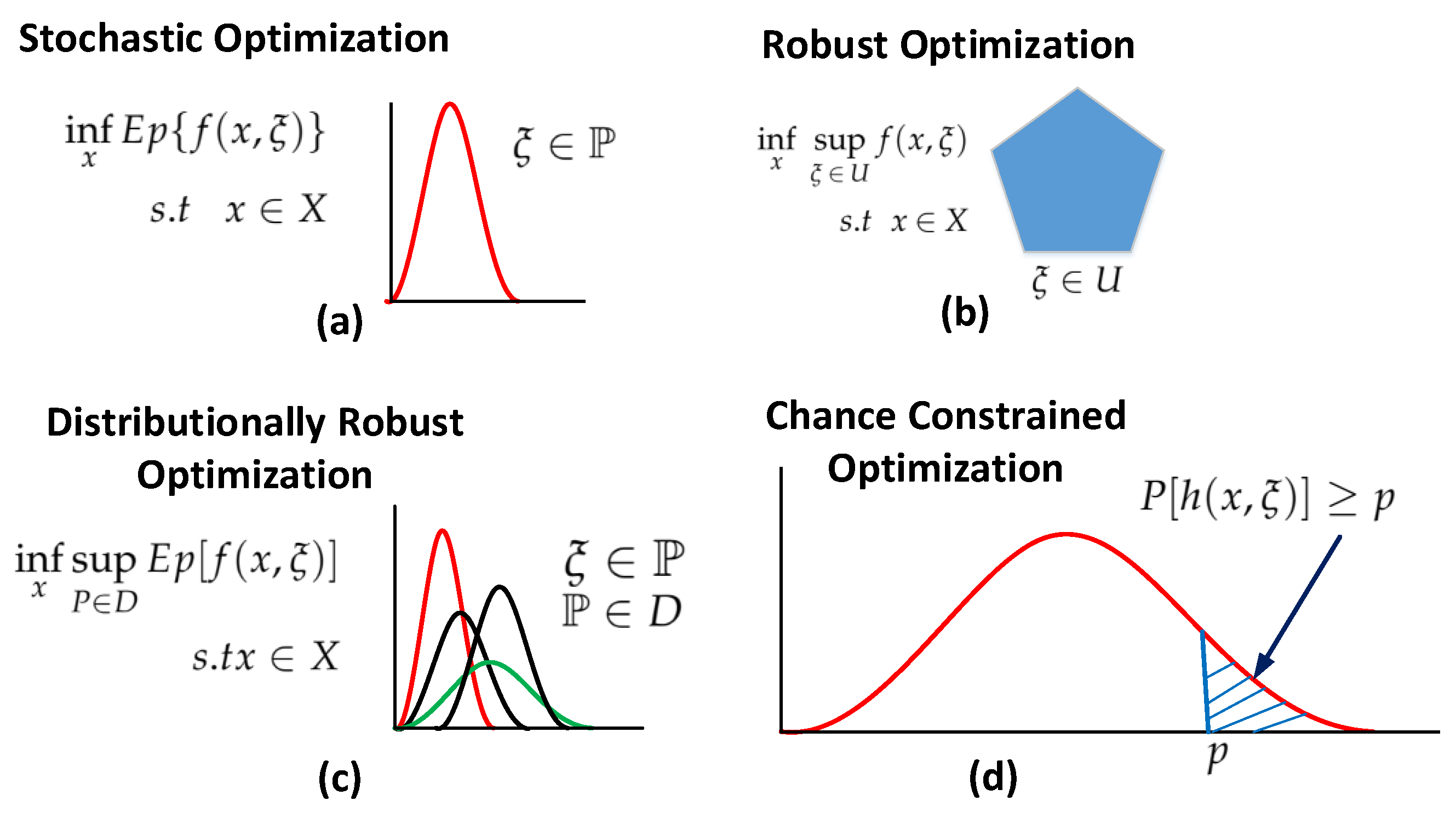
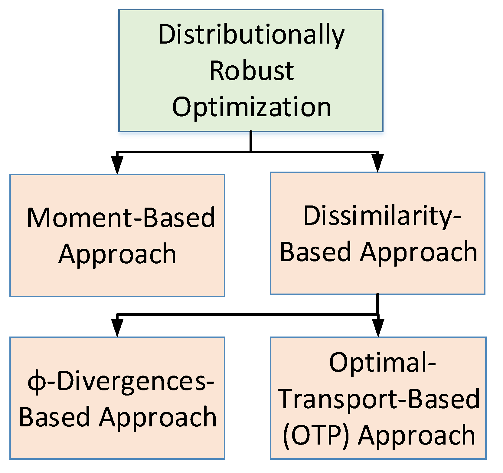
Table 1.
Summary of Related Survey Papers.
| Ref. | SO | RO | DRO | CC | AR | TN | OF | SA | Smart Power System |
|---|---|---|---|---|---|---|---|---|---|
| [25] | ✔ | ✔ | ✔ | ||||||
| [26] | ✔ | ✔ | ✔ | ||||||
| [27] | ✔ | ✔ | ✔ | ✔ | ✔ | ||||
| [28] | ✔ | ✔ | |||||||
| [29] | ✔ | ✔ | ✔ | ||||||
| [30] | ✔ | ✔ | |||||||
| [31] | ✔ | ✔ | ✔ | ||||||
| Our Review Paper | ✔ | ✔ | ✔ | ✔ | ✔ | ✔ | ✔ | ✔ | ✔ |
Table 2.
Applications of stochastic optimization and its problem type.
| References | Applications | LP | NLP | MILP | MISOCP | MIQP |
|---|---|---|---|---|---|---|
| [59] | HEM | × | ||||
| [61] | MEM | × | ||||
| [68] | OPF | × | ||||
| [62,63] | DRM | × | ||||
| [23,64] | ED | × | ||||
| [24,66] | UC | × | × | |||
| [60] | STG | × | ||||
| [65] | RDG | × |
Table 3.
Applications of robust optimization and its problem Type.
| Ref. | Applications | LP | NLP | MIP | MILP | MINLP | MIBLP | MISOCP | MIQP | QP |
|---|---|---|---|---|---|---|---|---|---|---|
| [69] | SGEM | × | ||||||||
| [70,71,72,73,75] | MEM | × | × | × | ||||||
| [90,91] | HEM | × | ||||||||
| [88,89,93] | DSM | × | × | × | ||||||
| [92,94] | PEV | × | × | |||||||
| [67,78,83,84,85,87,95,96,97,98,99,100,101,102,103,104] | UC | × | × | × | × | × | × | |||
| [105] | SGTD | × |
Table 4.
Objectives of robust optimization and its solution algorithms.
| Ref. | Objectives | CCG | AM | LDR | IPEA and MH | HE | BD | TOA | DD and IGDT | MPC and FPIM | BB | LM | QP | MCS | LOM and BMLM | IM |
|---|---|---|---|---|---|---|---|---|---|---|---|---|---|---|---|---|
| [92,106,107] | Minimize Generation Cost | × | × | |||||||||||||
| [89,91] | Minimize Electricity Cost | × | × | |||||||||||||
| [76] | Minimize Social Benefits Cost | × | × | |||||||||||||
| [73,77] | Minimize Microgrid Net Cost | × | × | |||||||||||||
| [90] | Minimize Comfort Violation | × | ||||||||||||||
| [72,78,85,111] | Minimize Operation Cost | × | × | × | ||||||||||||
| [67,71,75,81,82,83,84,86,98,110] | Minimize Overall Cost | × | × | × | × | × | × | × | ||||||||
| [93] | Minimize Electricity Payment | × | × | |||||||||||||
| [69,87] | Maximize Social Welfare | × | × | |||||||||||||
| [75] | Maximize Profits | × |
Table 5.
Application of chance constrained optimization and its problem type.
| Ref. | Applications | LP | NLP | MIP | MILP | MINLP | MIBLP | MISOCP | SOCP | MIQP |
|---|---|---|---|---|---|---|---|---|---|---|
| [115,116,117,118,142,143] | MEM | × | × | × | × | × | ||||
| [129] | HEM | × | ||||||||
| [119,120,121,123,124] | DEM | × | × | × | ||||||
| [127,128] | SDN | × | × | |||||||
| [125,126] | DSM | × | ||||||||
| [141] | PEV | × | ||||||||
| [138] | ED | × | ||||||||
| [130,131,133,134,135,136,137,144] | UC | × | × | × | × | × | × | |||
| [145] | GEM | × | ||||||||
| [146] | OPF | × | ||||||||
| [147] | OPGF | × |
Table 6.
Objectives of chance constrained optimization and the solution algorithms.
| Ref. | Objectives | SAA | AM | SBM | IPM | HE | BD and DE | HABC | POC | DD | SA | SVM | LR and IM | MDP | MCS | MDP | ADMM |
|---|---|---|---|---|---|---|---|---|---|---|---|---|---|---|---|---|---|
| [106,130] | Minimize Generation Cost | × | × | ||||||||||||||
| [133] | Constraints Satisfaction | × | |||||||||||||||
| [131,132] | Minimize Reserve Cost | × | × | ||||||||||||||
| [125] | Minimize Signal Price | × | |||||||||||||||
| [142] | Minimize Electricity Cost | × | |||||||||||||||
| [115,118,134,135] | Minimize Operating Cost | × | × | × | |||||||||||||
| [116,117,119,120,123,127,136,144,148] | Minimize Overall Cost | × | × | × | × | × | × | ||||||||||
| [121] | Minimize Thermal line losses | × | |||||||||||||||
| [128] | Minimize planning cost | × | |||||||||||||||
| [139] | Minimize Active Power Losses | × | × | ||||||||||||||
| [140] | Maximize payoff | × | |||||||||||||||
| [145] | Minimize Dispatch cost | × | |||||||||||||||
| [149] | Minimize Social cost | × |
Publisher’s Note: MDPI stays neutral with regard to jurisdictional claims in published maps and institutional affiliations. |
© 2022 by the authors. Licensee MDPI, Basel, Switzerland. This article is an open access article distributed under the terms and conditions of the Creative Commons Attribution (CC BY) license (https://creativecommons.org/licenses/by/4.0/).
Share and Cite
MDPI and ACS Style
Riaz, M.; Ahmad, S.; Hussain, I.; Naeem, M.; Mihet-Popa, L. Probabilistic Optimization Techniques in Smart Power System. Energies 2022, 15, 825. https://0-doi-org.brum.beds.ac.uk/10.3390/en15030825
AMA Style
Riaz M, Ahmad S, Hussain I, Naeem M, Mihet-Popa L. Probabilistic Optimization Techniques in Smart Power System. Energies. 2022; 15(3):825. https://0-doi-org.brum.beds.ac.uk/10.3390/en15030825
Chicago/Turabian StyleRiaz, Muhammad, Sadiq Ahmad, Irshad Hussain, Muhammad Naeem, and Lucian Mihet-Popa. 2022. "Probabilistic Optimization Techniques in Smart Power System" Energies 15, no. 3: 825. https://0-doi-org.brum.beds.ac.uk/10.3390/en15030825
Note that from the first issue of 2016, this journal uses article numbers instead of page numbers. See further details here.