
HPC Geophysical Electromagnetics: A Synthetic VTI Model with Complex Bathymetry


Barcelona Supercomputing Center (BSC), 08034 Barcelona, Spain
*
Author to whom correspondence should be addressed.
Energies 2022, 15(4), 1272; https://0-doi-org.brum.beds.ac.uk/10.3390/en15041272
Submission received: 12 January 2022
/
Revised: 26 January 2022
/
Accepted: 7 February 2022
/
Published: 10 February 2022
(This article belongs to the Special Issue Towards Exascale HPC and Data Intensive Algorithms in the Energy Industry)
Abstract
:We introduce a new synthetic marine model for 3D controlled-source electromagnetic method (CSEM) surveys. The proposed model includes relevant features for the electromagnetic geophysical community such as large conductivity contrast with vertical transverse isotropy and a complex bathymetry profile. In this paper, we present the experimental setup and several 3D CSEM simulations in the presence of a resistivity unit denoting a hydrocarbon reservoir. We employ a parallel and high-order vector finite element routine to perform the CSEM simulations. By using tailored meshes, several scenarios are simulated to assess the influence of the reservoir unit presence on the electromagnetic responses. Our numerical assessment confirms that resistivity unit strongly influences the amplitude and phase of the electromagnetic measurements. We investigate the code performance for the solution of fundamental frequencies on high-performance computing architectures. Here, excellent performance ratios are obtained. Our benchmark model and its modeling results are developed under an open-source scheme that promotes easy access to data and reproducible solutions.
1. Introduction
The Earth’s subsurface holds natural resources which are fundamental for local and regional development. Obtaining accurate images of water reservoirs, mineral, and energy sources deep below the surface is a crutial step for their management and exploitation. Geophysical imaging allows us to obtain detailed maps of the Earth’s interior. This is achieved by analyzing the deformations and electromagnetic (EM) fields measured at the surface. The EM modeling routines estimate the EM fields arising from induced electric currents in the Earth’s subsurface. The EM response to that excitation source depends on the electrical distribution of geological properties. From this dependence, it is possible to extract useful subsurface information to improve and reinforce reservoirs’ characterization and interpretation [1]. In consequence, EM approaches are now a well-established tool in geophysics, with applications in a wide range of fields including hydrocarbon and mineral exploration, reservoir monitoring, CO storage characterisation, geothermal reservoir imaging, water prospecting, and more.
Geophysical EM modeling is an active and dynamic research area. The most often used methods for resolving Maxwell’s equations are the Integral Equation method (IE; [2,3,4,5]), and different versions of the differential Equation (DE) method, such as Finite Difference (FD; [6,7,8,9,10,11]), Finite Elements (FE; [12,13,14,15]), and Finite Volume (FV; [16,17,18]). Furthermore, several approaches to accelerate the solution of Maxwell’s equations have been evaluated in different application contexts. Out of these approaches, the conjugate gradient method [19], vectorization techniques [20], multifrontal methods [13], and sparse matrix reordering schemes [21], stand out.
Several 3D modelers have been developed for mapping the subsurface through the study of the electrical conductivity/resistivity as a diagnostic physical property. Out of these modeling tools, custEM [22], emg3d [23], PETGEM [24], SimPEG [25], stand out. These modeling routines should be particularly sought for: (a) providing accurate solutions in a feasible runtime; (b) tackling problems efficiently; (c) bringing flexibility to cope with a variety of real-life models. The improvement of these modeling tools have a critical role in solving the next generation of geoscience challenges. These problems are complex, multidisciplinary, and require collaboration to understand and solve the physical equations, pre-process and post-process the associated data with physical experiments, and build interpretations from the analysis of the numerical results. These are the principal motivations of our work, together with the necessity for more reproducible modeling results.
This paper introduces a new model for 3D controlled-source electromagnetic method (CSEM) surveys. The proposed model includes large conductivity contrast with anisotropic (vertical transverse isotropy, VTI), and a complex bathymetry profile, making it challenging and ideal for addressing the topic of validation and for testing new algorithms and modeling routines. We have used the PETGEM code to compute the synthetic EM responses, which has proven to be an efficient large-scale modeling routine on cutting-edge high-performance computing (HPC) clusters. We acknowledge that the CSEM modeling methodology presented in this paper is well-established. However, the availability of data (resistivity model, input mesh, electromagnetic responses) for reproductively/verification purposes continues to be a limiting issue in the geophysical EM modeling community. To reverse this situation, the proposed model and numerical results are based on an open approach. Furthermore, we state that our open data and benchmark are valid and useful for different application contexts (e.g., oil and gas, geothermal exploration, CO sequestration, among others) and passive-source EM schemes such as the Magnetotelluric method (MT). This transversality feature favors the expertise transfer from mature energy applications (e.g., oil and gas) to emerging energy applications (e.g., geothermal exploration).
The rest of the paper is organized as follows. Section 2 provides a comprehensive description of the mathematical background of the CSEM forward modeling. In Section 3, we present details about the PETGEM code and its HPC workflow for EM modeling. In Section 4, we provide a detailed description of the proposed marine CSEM model. In addition, we perform several PETGEM simulations to investigate the EM field pattern and the code performance on HPC architectures. We conclude with a discussion in Section 5. We provide summary remarks in Section 6.
2. EM Modeling Theory
The EM forward modeling problem is mathematically described by the frequency-domain Maxwell’s equations in diffusive form, written as [26]
where , are the electric and magnetic fields, respectively; , are the electric and magnetic sources, respectively; i is the imaginary unit; denotes the angular frequency; is the constant free-space magnetic permeability due Earth materials are not magnetizable; denotes the constant model permittivity; and is the variable electric conductivity tensor. According to the type of the excitation source, the EM forward problem may be classified as active-source (e.g., CSEM) and passive-source (e.g., MT) methods. In this paper, we focus on the CSEM method and we provide a brief outline and details essential for understanding it. For a comprehensive introduction to the CSEM and MT methods, we refer to [24,27,28,29].
In the field of CSEM modeling, it is commonly to formulate the Equations (1) and (2) in terms of total electric field. After substituting Equation (1) into Equation (2), we obtain
which is known as the curl-curl formulation of the problem in terms of the total electric field. In Equation (3) we impose the usual assumption . When CSEM methods are considered, the electric source corresponds to a electric dipole oscillating at a single frequency. Furthermore, no magnetic sources are generated, thus .
The numerical approximation of the EM fields by the High-order Edge Finite Element Method (HEFEM) requires the variational form of Equation (3). For more details and proofs about this high-order numerical discretization, we refer to [24,30,31]. For our modeling purposes the computational domain is truncated by homogeneous Dirichlet boundary conditions.
3. HPC Workflow for EM Modeling
We have implemented the above algorithm and numerical schemes in a fully distributed fashion using Python 3 language, mpi4py, and petsc4py packages. The net result is the PETGEM code, which is an EM tool to solve both active-source and passive-source EM methods in 3D arbitrary marine/land problems under anisotropic conductivities. A triple helix model based on global polynomial variants (p-refinement), tailored tetrahedral meshes (h-refinement), and massively parallel computations, stand out as the main distinguishing factors of PETGEM with respect to other modeling routines.
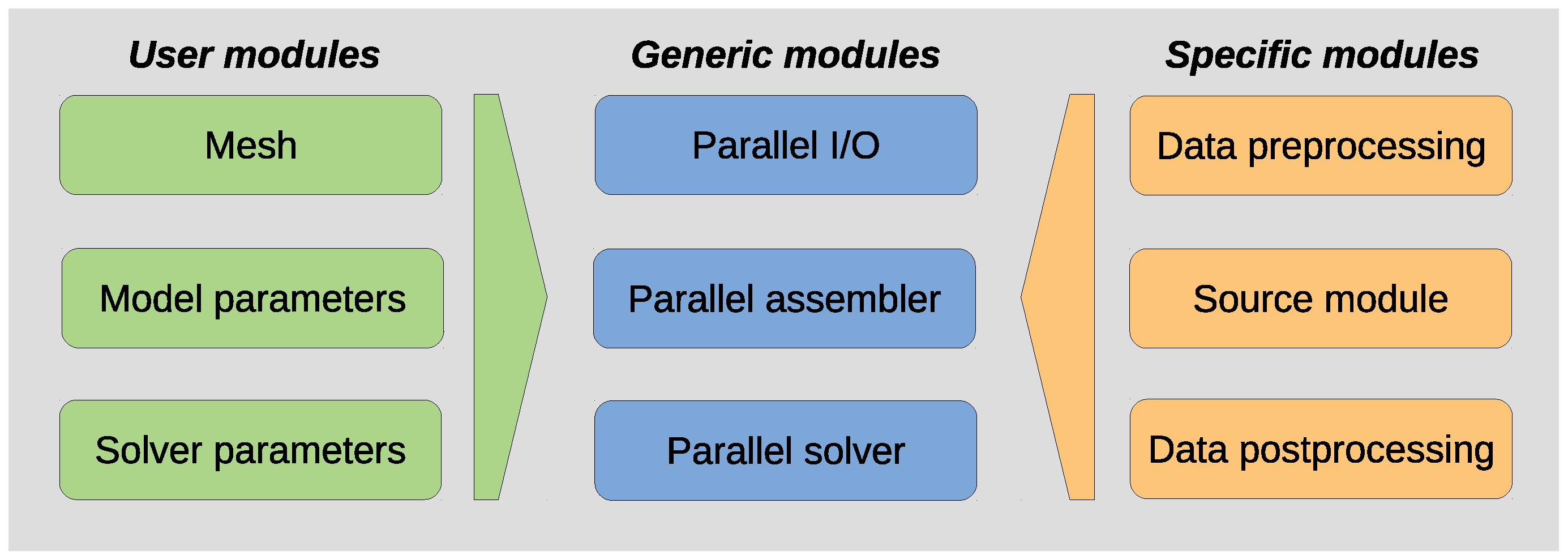
The overall PETGEM software stack is shown in Figure 1. To point out the virtues of this code environment, we summarize the essential aspects its main modules:
- Provided by user: this set of modules provides functionalities to parse user parameters regarding the physics of the EM problem to be solved (e.g., frequency and conductivity model), the solver type (e.g., direct or iterative), and the mesh file.
- Specific modules: depending on the source type (active or passive), these modules provide support to define the modeling work-flow. They are in charge of data preprocessing (e.g., import mesh file and compute its associated data structures such as dof connectivity) and data postprocessing (e.g., computation of EM responses on a set of points and output of files for posterior analysis).
- Generic modules: Once the modeling’s specifics are provided, these modules perform the assembly and solution of the linear system of Equations (LSE). These tasks are entire parallel by using the mpi4py and petsc4py packages.
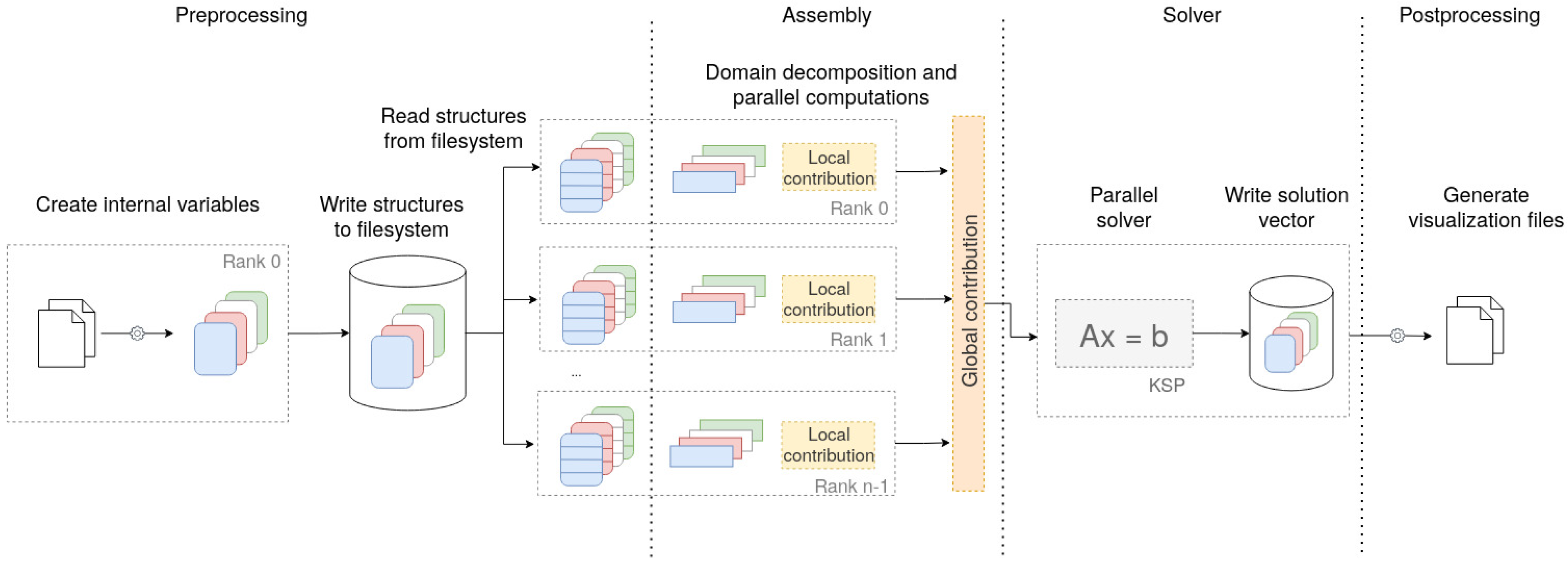
The software stack mentioned above is modular, simple, and flexible. Furthermore, its HPC support make it appropriate to be used in an inversion procedure scheme (e.g., iterative or stochastic). For clarity, Figure 2 depicts the block diagram overview of the PETGEM code. This diagram can be summarize as follows:
- Following the input parameters, a set of data are preprocessed (mesh, conductivity model and receivers positions).
- A problem instance is created.
- The domain decomposition is performed, and the main data structures are created.
- Parallel assembling of the LSE ().
- The LSE is solved in parallel by calling a ksp PETSc object.
- Interpolation of electromagnetic responses and post-processing parallel stage.
We state that our modeling work-flow is open-source under the BSD-3 license. Please notice that the majority of the current tools for 3D geo-electromagnetic modeling lack this last feature, which makes it hard for other researchers to assess whether their underlying formulation and algorithmics suit whichever computing architecture those tools are deployed on. However, our parallel code is entirely open-source. Thus, it allows for a complete exploration of its numerical formulation and implementation. This feature eases its efficient deployment on different computational architectures. PETGEM code is hosted and versioned in a public on-line repository with unit-testing and continuous integration control. This open model engages users to submit and track issues, promoting the building of global communities around not only PETGEM project but also for a broader audience since it fosters research at the intersection of EM modeling, high-order numerical methods, and HPC.
4. Numerical Experiments
We design a new synthetic 3D CSEM model that integrates relevant features for the EM community. More concretely, the model under consideration includes large conductivity contrast with VTI, complex seabed profile, and realistic domain dimensions. There are no semi-analytical solutions for such a resistivity model to verify our synthetic EM responses, and we can only corroborate them by comparing different numerical approximations. On the off chance that distinctive discretizations and implementations of Maxwell’s equations surrender the same result, it gives certainty in their numerical precision. Then, for all experiments, we consider a normalized root-mean square difference (NRMSD) between two synthetic responses and , given by
to which we allude as basically the normalized difference through the paper.
The simulations have been performed on Marenostrum supercomputer, which is based on Intel Xeon Platinum processors from the Skylake generation. It is a Lenovo system composed of SD530 Compute Racks, an Intel Omni-Path high performance network interconnect and running SuSE Linux Enterprise Server as operating system. This general purpose supercomputer consists of 48 racks housing 3456 nodes with a grand total of 165,888 processor cores and 390 Terabytes of main memory. Compute nodes are equipped with:
- Two socket Intel Xeon Platinum 8160 CPU with 24 cores each at 2.10 GHz for a total of 48 cores per node
- L1d 32 K; L1i cache 32 K; L2 cache 1024 K; L3 cache 33,792 K
- Total of 96 GB of main memory 1.880 GB/core, 12 × 8 GB 2667 Mhz DIMM (216 nodes high memory, 10,368 cores with 7.928 GB/core)
- A 100 Gbit/s Intel Omni-Path HFI Silicon 100 Series PCI-E adapter
- A 10 Gbit Ethernet
- A 200 GB local SSD available as temporary storage during jobs
The processors support well-known vectorization instructions such as SSE, AVX up to AVX–512. We point out that in the corresponding PETGEM website, the data model (e.g., geometry, mesh file, parameters file) and modeling results can be download for comparison purposes.
4.1. 3D VTI Marine Model with Bathymetry (3D-VTI-B)
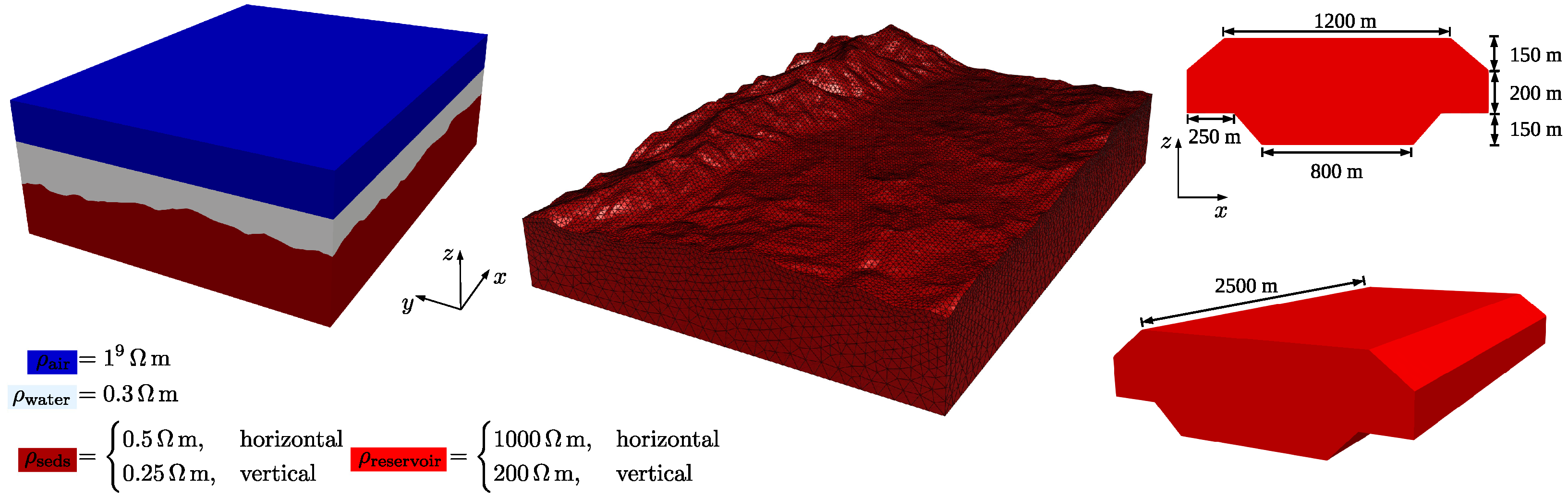
We propose a synthetic 3D VTI model that includes large conductivity contrast and challenging bathymetry profile. The model, depicted in Figure 3, is comprised of an air layer (m) with constant thickness of km. The seawater is an isotropic medium (m) where the sea-bottom depth ranges from m to m. The subsurface consists of one sedimentary formation with VTI (m and m). Finally, a resistivity unit (m and m) denoting hydrocarbon is embedded at the sediments layer. The horizontal extent of the hydrocarbon reservoir is km × km. The model encompasses a km × km × km volume with its origin at km, km, km. We use an x-oriented electric dipole at Hz located above the seafloor (km, km, km). The transmitter moment is Am.
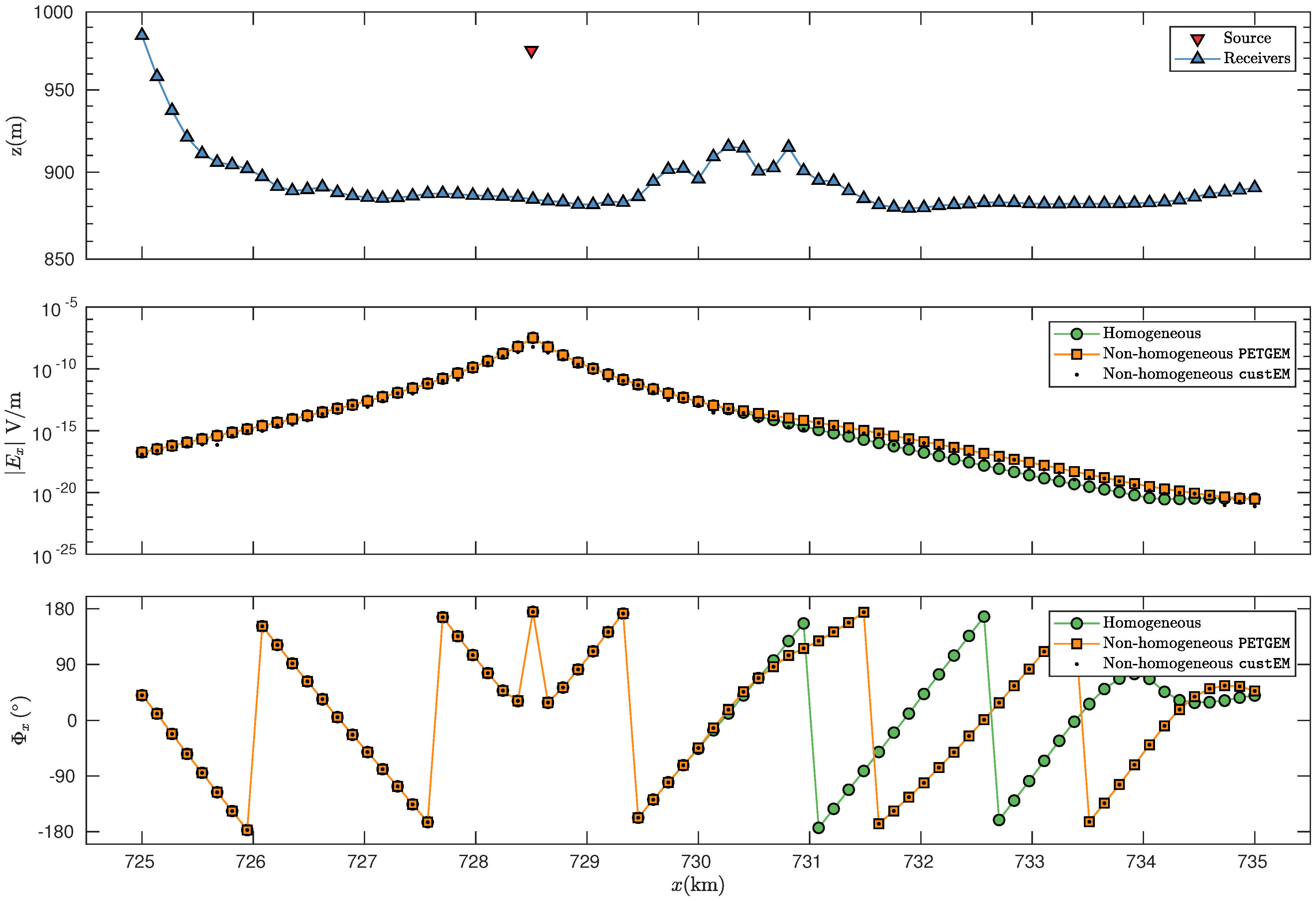
We based our computational model design on the skin-depth () principle, defined as the effective depth of penetration of EM energy in a conducting medium, where the amplitude of a plane wave in a whole space has been attenuated to or [24]. For this modeling test, the value is approximately km in terms of the host resistivity of reservoir. By using this parameter, and following the rules proposed by [31], seventy-five measuring sites are located along the x-axis in the range km with a receiver distance of m, directly above the seafloor ( km). Given the resistivity model and reservoir dimensions, we state that this measuring sites configuration satisfies the accuracy and detection requirements of the resistive body. Furthermore, we design an -adapted mesh for basis order . The resulting mesh consists of 1,918,108 degrees of freedom (dof).
4.2. EM Fields Analysis
To investigate the impact of the reservoir presence on the measured EM responses, we compare the numerical solutions for a homogeneous model () against a non-homogeneous model (, which is equivalent to the initial configuration). We compute custEM and PETGEM solutions. A multifrontal parallel solver MUMPS has been used to solve the resulting LSE for the unknown EM fields. The MUMPS solver is supported by both EM modeling routines.
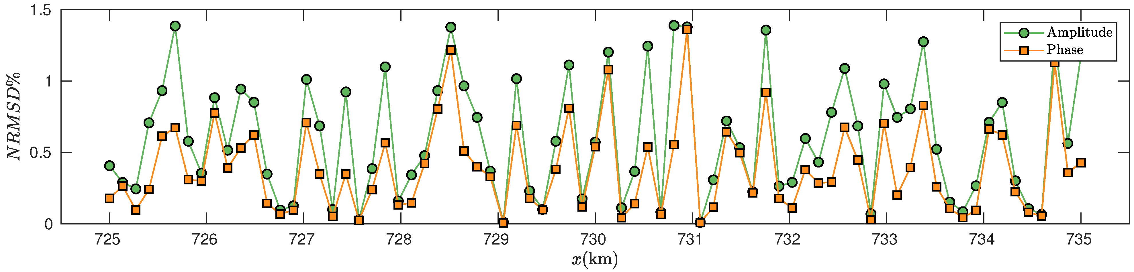
For both homogeneous and non-homogeneous models, Figure 4 shows the obtained electric field amplitude and phase along the in-line receiver profile. Here, it can be seen that both numerical approximations are similar for receivers located far from the resistivity unit vicinity (km to km). However, for the case where the reservoir is present, the electric field amplitudes and phases are only modified close the resistivity unit, which corresponds to a local effect (km to km). More concretely, for the non-homogeneous case, the and are modified by different orders of magnitude along with the in-line profile. An excellent agreement between the custEM and PETGEM solutions can be seen. The synthetic EM responses have mostly a relative error of less than 1–2%. The cross-validation of the numerical approximations for non-homogeneous yields an excellent agreement with NRMSD within a few per cents. For clarity, Figure 5 shows the obtained NRMSD for amplitude and phase responses. This EM pattern is as expected and has been broadly studied in previous works for several and different CSEM setups [28,29]. Nonetheless, we acknowledge that the electric field pattern depends on the input model setup (e.g., source type, fundamental frequency, resistivity, depth of station where EM fields are measured). For a comprehensive analysis of the impact of these factors on EM field behaviour we refer to [32].
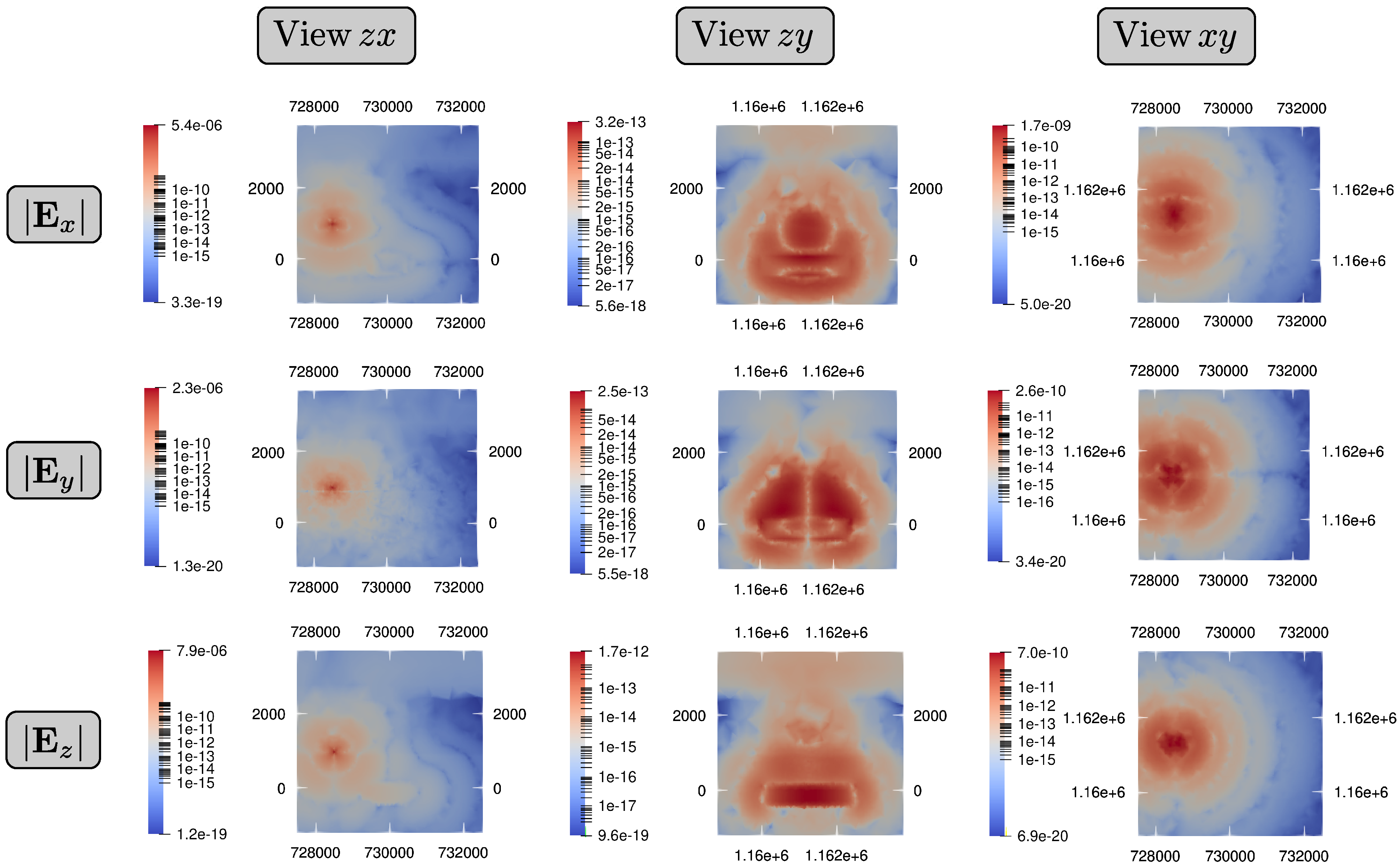
We compute the electric field amplitude around the reservoir location to present a full analysis of the 3D EM behavior. Figure 6 shows the EM responses for three view profiles. The amplitude distributions depicted in the first column of Figure 6 illustrate filed perturbations due to the presence of the resistivity unit. The second column of Figure 6 shows additional electric field perturbations due to the VTI. Finally, the third column of Figure 6 shows the amplitude variations caused by the reservoir presence. We point out that the significant differences in the electric field components imply that the vertical EM field is more susceptible to the perturbations of the resistivity model and is more informative than the in-line EM field for laterally heterogeneous targets. Then, this feature could be employed to get better signal-to-noise trade-offs on stations near to the vicinity of the resistivity unit [32]. Nonetheless, we acknowledge that this EM field pattern is reduced and only effective close to the reservoir location (km to km). Thus, its effect depends on where the reservoir unit is located with respect to the source. Nevertheless, the effect on EM measurements should be considered to avoid misunderstanding interpretations [32].
4.3. Performance Analysis
As a second experiment, we study the parallel performance of the PETGEM code for the solution of the proposed 3D-VTI-B model. For this test, we solve five fundamental frequencies on adapted meshes for basis order . The obtained grid statistics are summarized in Table 1. We state that the design of adapted meshes can be advantageous for the solution of the CSEM test under study. A close assessment of Table 1 shows that the number of tetrahedal elements and dof in the mesh remains constant for all frequencies. Further, the run-time to reach the solution for each fundamental frequency is almost constant. The iterative GMRES solver provided by PETSc has been used to solve the LSE.
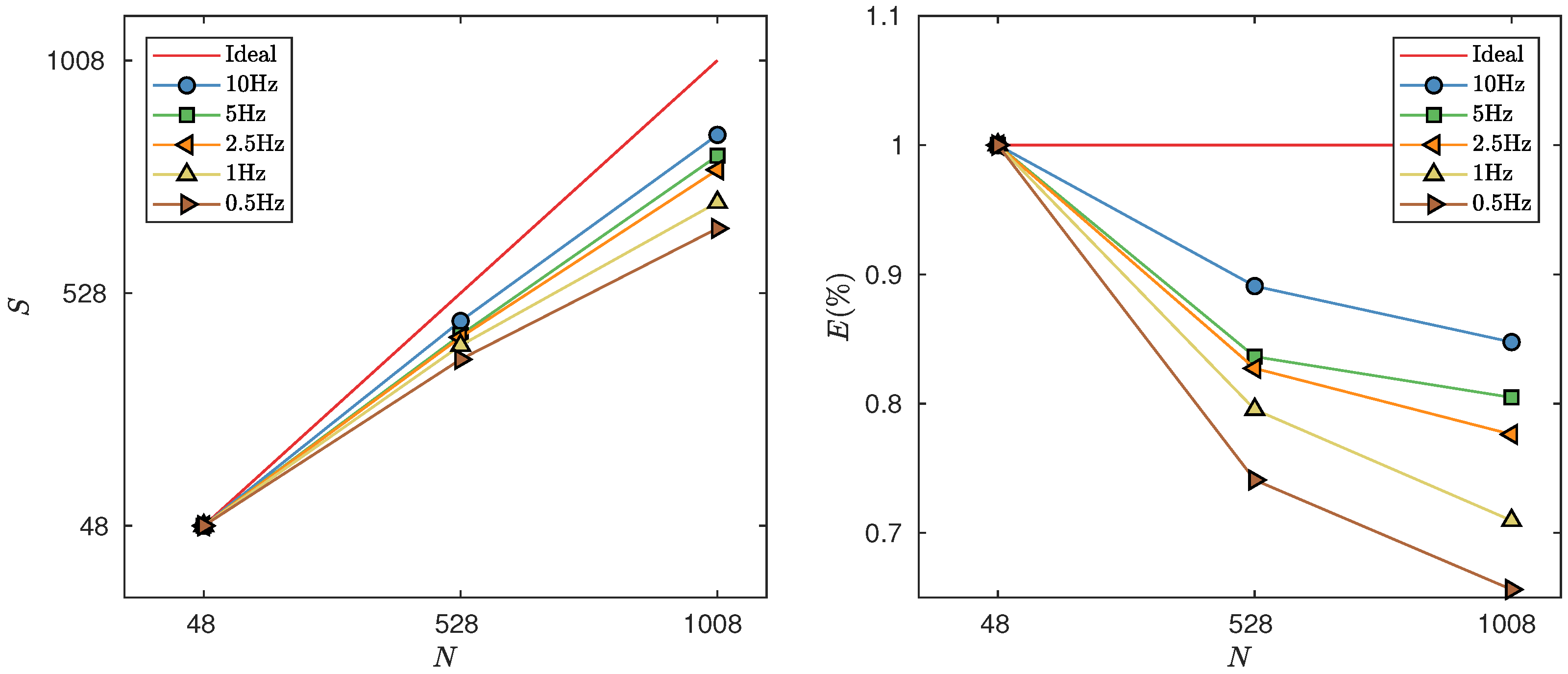
We investigate two main performance metrics on distributed-memory clusters, namely the speed-up ratios and parallel efficiency of the code. We analyze how the run-time varies with the number of CPU N (e.g., 48, 528, 1008 CPUs) for a fixed total problem size. For more details about these performance metrics, we refer to [31]. The obtained performance ratios are shown in Table 1. Figure 7 shows the performance indicators for each target frequency. We achieved a near linear speed-up ratio for up to 528 processors. For a higher number of processors, the performance decreases mainly because the execution becomes dominated by the communication task during the solver phase. However, the scalability ratio keeps increasing up to 1008 CPUs.
Furthermore, in our numerical results, better performance metrics for high-frequency solutions can be observed. We point out that these performance ratios depend primarily on the parallel solver features. Because we employ PETSc solver implementations, no particular work was undertaken to reduce run-time, as this is an completely different goal. However, these numerical results indicate a remarkable benefit when parallel executions are employed (similar conclusions to that described in [31,32]).
5. Discussion
The development and implementation of routines for 3D geo-electromagnetic modeling has expanded within the last decade. Consequently, nowadays, there are diverse tools available to solve arbitrarily models of the 3D geo-electromagnetic modeling. However, most of the existing routines for computation of synthetic EM responses absence an open-source environment, which makes it difficult for other EM modellers or developers to study, adjust, and expand the code capabilities to their own requirements. Furthermore, most of the data-sets are proprietary or not available in open repositories for free use. Previous ideas are the principal motivations for this paper and the introduction of a 3D-VTI-B model.
The proposed model is realistic in terms of dimensions and physical parameters (e.g., resistivity model with high contrasts and large range of fundamental frequencies). We compute the solutions for the 3D-VTI-B model. Overall, we obtain an excellent match between the numerical approximations obtained with custEM and PETGEM. The main purpose of the first test is to study the impact of the reservoir presence on the measured EM responses. The cross-validation between custEM and PETGEM yields a similar EM pattern (the obtained synthetic EM responses have mostly a relative misfit of less than 1–3%). Thus, we consider these numerical results correct because comparing different modeling routines that use different numerical schemes is proper to address the topic of verification.
The 3D-VTI-B model simulations performed on tailored meshes yields a positive impact in terms of number of dofs required to satisfy a quality criterion (e.g., threshold error in synthetic EM responses). In compliance with one of the principal outcome of this paper, the grid design is a difficult and laborious task, but its expertise is critical for time to come modeling rouyine developments (e.g., implementation of 3D EM inversion algorithms). We design tailored meshes based on the skin-depth parameter as the principal quality factor to decide the characteristic grid sizes. Such griding strategy consider the behavior of EM fields computation with its diffusive pattern. The main findings of this work corroborate that tailored meshes are required to improve the algorithm’s adaptability and supply accurate EM responses in a viable computation time. The numerical results of the 3D-VTI-B model corroborate that the strict employment of tailored griding rules can be effective for 3D geo-electromagnetic modeling (e.g., the number of unknows and run-time is constant for each fundamental frequency, see Table 1). On top of that, we encourage the design and use of tailored meshes by the EM modellers.
We state that although the model we present is synthetic, it is relevant for the geo-electromagnetic community and can be used as benchmark for new modeling routines. We also point out that, given the results of the numerical tests, there is no reason to think that the proposed algorithm does not work well with real data beyond the model limitations.
Regarding the computational performance, the chosen solver is the principal discriminator. We employ the iterative GMRES solver to compute the numerical solutions for the introduced resistivity model. In general, a considerable run-time improvement can be seen by performing a strong scaling test. We state that the improvement of reported run-time has been achieved through HPC, a differentiating PETGEM feature concerning the rest of EM modeling tools. Our performance study shows that high-frequencies achieve better performance ratios than low-frequencies.
6. Conclusions
We have presented a new 3D VTI model (3D-VTI-B) that includes significant conductivity contrast and a challenging bathymetry profile. We, carried out several simulations to analyze the EM field behavior and the code performance. The relevance of these studies is based on two main arguments. First, the solution to the next generation of geoscience problems requires accurate, flexible, and efficient modeling routines. Thus, to address the validation of the computational tools, models that exhibit realistic setups are needed. Second, it is well known the scarcity of more open and reproducible numerical approximations in the realm of geophysical EM. The challenges mentioned above are the principal motivations of this work.
Because the proposed model has no semi-analytical solution, we validate our numerical approximations by comparing different synthetic EM responses. Then, we compare the computed fields of two different open-source 3D EM modeling routines. We study the resistivity unit effect by considering homogeneous and non-homogeneous configurations. The cross-validation of both synthetic EM responses shows a NRMSD of a few per cent (1–2%). For an in-depth analysis, we have generated 3D views of the EM field pattern. Numerical approximations corroborate that reservoir presence strongly alters EM fields, but its impact is restricted to the near region of the resistivity unit. Furthermore, in our experiments, the vertical EM field is more sensitive to the variations of the resistivity model and, in consequence, more informative than the in-line EM responses. Still, the pattern of EM fields should be investigated and analyzed to avoid misunderstanding conclusions.
PETGEM code offers excellent computational performance ratios. The obtained performance metrics are consistent with previously published results. Furthermore, our previously published tailored gridding strategy has been proved in the presence of complex bathymetry and for modeling different fundamental frequencies. Our mesh design approach demonstrated that can deal with challenging bathymetry and realistic physical parameters.
The whole set of these numerical results presented in this work show that PETGEM code features fulfill modeling requisites of practical setups in the context of HPC geophysical electromagnetics. We acknowledge that validating and testing 3D algorithms and codes are difficult tasks. Then, it is fundamental to have benchmark models that are developed under an open-source scheme that promotes easy access to data and reproducible solutions. Therefore, in the corresponding PETGEM website and Zenodo, the dataset and all results can be download for comparison purposes. We trust that these numerical dataset may be helpful for the geophysical community interested in HPC geoelectromagnetics. We stir the community to design more models, modeling tools, and numerical experiments under an open-source approach.
Author Contributions
O.C.-R. Conceived the study, Contributed to the parallel implementation, math background, mesh generation, PETGEM simulations, Wrote the manuscript. J.d.l.P.: Analyzed and interpreted the modeling results, Super vised the overall study, Critically revised the manuscript. J.M.C.: Analyzed and interpreted the modeling results, Critically revised the manuscript. All authors have read and agreed to the published version of the manuscript.
Funding
This research received no external funding.
Institutional Review Board Statement
Not applicable.
Informed Consent Statement
Not applicable.
Data Availability Statement
The resulting CSEM responses of the PETGEM code for the 3D-VTI-B model, as well as all files to rerun the model with the PETGEM and reproduce the shown results are available at Zenodo (10.5281/zenodo.5842270). The PETGEM code is freely available at the home page project (https://petgem.bsc.es), at the PyPI repository (https://pypi.org/project/petgem), at the GitHub site (https://github.com/ocastilloreyes/petgem), or by requesting it from the author ([email protected]). In all cases, the code is supplied to ease the immediate execution on Linux platforms. User’s manual and technical documentation (developer’s guide) are provided in the PETGEM archive.
Acknowledgments
The work of O.C-R., conducted in the frame of PIXIL project, has been 65% cofinanced by the European Regional Development Fund (ERDF) through the Interreg V-A Spain-France-Andorra program (POCTEFA2014–2020). POCTEFA aims to reinforce the economic and social integration of the French-Spanish-Andorran border. Its support is focused on developing economic, social and environmental cross-border activities through joint strategies favouring sustainable territorial development. BSC authors have received funding from the European Union’s Horizon 2020 programme under the Marie Sklodowska-Curie grant agreement N 777778. Furthermore, the development of PETGEM has received funding from the European Union’s Horizon 2020 programme, grant agreement N 828947, and from the Mexican Department of Energy, CONACYT-SENER Hidrocarburos grant agreement N B-S-69926. We would like to thank Jazmin Ester Gell for plotting of block diagram overview of PETGEM.
Conflicts of Interest
The authors declare no conflict of interest.
References
- Castillo-Reyes, O.; Modesto, D.; Queralt, P.; Marcuello, A.; Ledo, J.; Amor-Martin, A.; de la Puente, J.; García-Castillo, L.E. 3D magnetotelluric modeling using high-order tetrahedral Nédélec elements on massively parallel computing platforms. Comput. Geosci. 2022, 1, 105030. [Google Scholar] [CrossRef]
- Raiche, A.P. An integral equation approach to three-dimensional modelling. Geophys. J. Int. 1974, 1, 363–376. [Google Scholar] [CrossRef] [Green Version]
- Hursán, G.; Zhdanov, M.S. Contraction integral equation method in three-dimensional electromagnetic modeling. Radio Sci. 2002, 1, 1–13. [Google Scholar] [CrossRef] [Green Version]
- Zhdanov, M.S.; Lee, S.K.; Yoshioka, K. Integral equation method for 3D modeling of electromagnetic fields in complex structures with inhomogeneous background conductivity. Geophysics 2006, 71, G333–G345. [Google Scholar] [CrossRef]
- Tehrani, A.M.; Slob, E. Fast and accurate three-dimensional con- trolled source electromagnetic modelling. Geophys. Prospect. 2010, 58, 1133–1146. [Google Scholar]
- Kruglyakov, M.; Bloshanskaya, L. High-performance parallel solver for integral equations of electromagnetics based on Galerkin method. Math. Geosci. 2016, 49, 751–776. [Google Scholar] [CrossRef] [Green Version]
- Wang, T.; Hohmann, G.W. A finite-difference, time-domain solution for three-dimensional electromagnetic modeling. Geophysics 1993, 58, 797–809. [Google Scholar] [CrossRef] [Green Version]
- Druskin, V.; Knizhnerman, L. Spectral approach to solving three-dimensional Maxwell’s diffusion equations in the time and frequency domains. Radio Sci. 1994, 1, 937–953. [Google Scholar] [CrossRef]
- Mackie, R.L.; Smith, J.T.; Madden, T.R. Three-dimensional electro-magnetic modeling using finite difference equations: The magnetotelluric example. Radio Sci. 1994, 29, 923–935. [Google Scholar] [CrossRef]
- Streich, R. 3D finite-difference frequency-domain modeling of controlled-source electromagnetic data: Direct solution and optimization for high accuracy. Geophysics 2009, 74, F95–F105. [Google Scholar] [CrossRef]
- Commer, M.; Newman, G. A parallel finite-difference approach for 3D transient electromagnetic modeling with galvanic sources. Geophysics 2004, 69, 1192–1202. [Google Scholar] [CrossRef] [Green Version]
- Schwarzbach, C.; Börner, R.-U.; Spitzer, K. Three-dimensional adaptive higher order finite element simulation for geoelectromagnetics—A marine CSEM example. Geophys. J. Int. 2011, 1, 63–74. [Google Scholar] [CrossRef] [Green Version]
- da Silva, N.V.; Morgan, J.V.; MacGregor, L.; Warner, M. A finite element multifrontal method for 3D CSEM modeling in the frequency domain. Geophysics 2012, 77, E101–E115. [Google Scholar] [CrossRef]
- Grayver, A.V.; Streich, R.; Ritter, O. Three-dimensional parallel distributed inversion of CSEM data using a direct forward solver. Geophys. J. Int. 2013, 193, 1432–1446. [Google Scholar] [CrossRef] [Green Version]
- Zhang, Y.; Key, K. MARE3DEM: A three-dimensional CSEM inversion based on a parallel adaptive finite element method using unstructured meshes. In SEG Technical Program Expanded Abstracts; Onepetro: Dallas, TX, USA, 2016; pp. 1009–1013. [Google Scholar]
- Madsen, N.K.; Ziolkowski, R.W. A three-dimensional modified finite volume technique for Maxwell’s equations. Electromagnetics 1990, 10, 147–161. [Google Scholar] [CrossRef]
- Clemens, M.; Weiland, T. Discrete electromagnetism with the finite integration technique. PIER 2001, 32, 65–87. [Google Scholar] [CrossRef] [Green Version]
- Jahandari, H.; Farquharson, C.G. A finite-volume solution to the geophysical electromagnetic forward problem using unstructured grids. Geophysics 2014, 79, E287–E302. [Google Scholar] [CrossRef]
- Newman, G.A.; Commer, M.; Carazzone, J.J. Imaging CSEM data in the presence of electrical anisotropy. Geophysics 2010, 75, F51–F61. [Google Scholar] [CrossRef]
- Sommer, M.; Hölz, S.; Moorkamp, M.; Swidinsky, A.; Heincke, B.; Scholl, C.; Jegen, M. GPU parallelization of a three dimensional marine CSEM code. Comput. Geosci. 2013, 58, 91–99. [Google Scholar] [CrossRef]
- Hong, C.; Sukumaran-Rajam, A.; Nisa, I.; Singh, K.; Sadayappan, P. Adaptive sparse tiling for sparse matrix multiplication. In Proceedings of the 24th Symposium on Principles and Practice of Parallel Programming, Washington, DC, USA, 16–20 February 2019; pp. 300–314. [Google Scholar]
- Rochlitz, R.; Skibbe, N.; Günther, T. custEM: Customizable finite element simulation of complex controlled-source electromagnetic data. Geophysics 2019, 84, F17–F33. [Google Scholar] [CrossRef]
- Werthmüller, D. An open-source full 3D electromagneticmodeler for 1D VTI media in Python: Empymod. Geophysics 2017, 82, WB9–WB19. [Google Scholar] [CrossRef]
- Castillo-Reyes, O.; de la Puente, J.; Cela, J.M. PETGEM: A parallel code for 3D CSEM forward modeling using edge finite elements. Comput. Geosci. 2018, 119, 123–136. [Google Scholar] [CrossRef] [Green Version]
- Heagy, L.J.; Cockett, R.; Kang, S.; Rosenkjaer, G.K.; Olden-burg, D.W. A framework for simulation and inversion in electromagnetics. Comput. Geosci. 2017, 107, 1–19. [Google Scholar] [CrossRef]
- Zhdanov, M.S. Geophysical Electromagnetic Theory and Methods; Elsevier: Amsterdam, The Netherlands, 2009; Volume 43, ISBN 9780444529633. [Google Scholar]
- Nam, M.J.; Kim, H.J.; Song, Y.; Lee, T.J.; Son, J.; Suh, J. 3D magnetotelluric modelling including surface topography. Geophys. Prospect. 2007, 55, 277–287. [Google Scholar] [CrossRef]
- Constable, S. Ten years of marine CSEM for hydrocarbon exploration. Geophysics 2010, 5, 75A67–75A81. [Google Scholar] [CrossRef] [Green Version]
- Kerry, K.; Ovall, J. A parallel goal-oriented adaptive finite element method for 2.5-D electromagnetic modelling. Geophys. J. Int. 2011, 1, 137–154. [Google Scholar]
- Jin, J. The Finite Element Method in Electromagnetics, 2nd ed.; Wiley: New York, NY, USA, 2002. [Google Scholar]
- Castillo-Reyes, O.; de la Puente, J.; García-Castillo, L.E.; Cela, J.M. Parallel 3-D marine controlled-source electromagnetic modelling using high-order tetrahedral Nédélec elements. Geophys. J. Int. 2019, 1, 39–65. [Google Scholar] [CrossRef]
- Castillo-Reyes, O.; Queralt, P.; Marcuello, A.; Ledo, J. Land CSEM Simulations and Experimental Test Using Metallic Casing in a Geothermal Exploration Context: Vallès Basin (NE Spain) Case Study. IEEE Trans. Geosci. Remote Sens. 2021, 60, 1–13. [Google Scholar] [CrossRef]
Figure 1.
Environment overview. This work-flow supports both 3D CSEM and MT survey setups.

Figure 2.
Block diagram overview of PETGEM code.

Figure 3.
Synthetic 3D VTI marine model with bathymetry. A 3D view of the complex seabed and the reservoir unit are provided. The resistivity values for each material are also given.
Figure 3.
Synthetic 3D VTI marine model with bathymetry. A 3D view of the complex seabed and the reservoir unit are provided. The resistivity values for each material are also given.

Figure 4.
Electric field responses for in-line profile of the synthetic 3D-VTI-B model depicted in Figure 3. Details of the seabed profile with transmitter and receivers positions are depicted in the top row. The amplitude and phase are depicted in the middle and bottom row, respectively. Homogeneous and non-homogeneous medium are compared.

Figure 5.
NRMSD for amplitude and phase depicted in Figure 4. Non-homogeneous setup of 3D-VTI-B model is compared.
Figure 5.
NRMSD for amplitude and phase depicted in Figure 4. Non-homogeneous setup of 3D-VTI-B model is compared.

Figure 6.
Electric field amplitude response of the 3D-VTI-B model around the reservoir unit. Three view profiles of the vector electric field components are given.
Figure 6.
Electric field amplitude response of the 3D-VTI-B model around the reservoir unit. Three view profiles of the vector electric field components are given.

Figure 7.
Performance results for the 3D-VTI-B model. For each fundamental frequency, the number of CPU N is plotted versus speed-up S (left-panel) and parallel efficiency ratio E (right-panel). The solid red line shows the theoretical ideal performance supposing 100% parallel efficiency.
Figure 7.
Performance results for the 3D-VTI-B model. For each fundamental frequency, the number of CPU N is plotted versus speed-up S (left-panel) and parallel efficiency ratio E (right-panel). The solid red line shows the theoretical ideal performance supposing 100% parallel efficiency.


Table 1.
Statistics of adapted meshes and performance results for 3D-VTI-B model. The frequency (Hz), number of elements, number of dof, run-time (minutes), speed-up S, and parallel efficiency E (%) for five relevant simulations are given.
Table 1.
Statistics of adapted meshes and performance results for 3D-VTI-B model. The frequency (Hz), number of elements, number of dof, run-time (minutes), speed-up S, and parallel efficiency E (%) for five relevant simulations are given.
| Frequency | Elements | Dof | Run-Time | S | E | ||||||
|---|---|---|---|---|---|---|---|---|---|---|---|
| 48 | 528 | 1008 | 48 | 528 | 1008 | 48 | 528 | 1008 | |||
| 10 | 602,593 | 3,678,324 | 88.85 | 9.06 | 4.99 | - | 9.8 | 17.79 | - | 89.09 | 84.76 |
| 5.0 | 615,378 | 3,737,031 | 76.85 | 8.35 | 4.54 | - | 9.2 | 16.90 | - | 83.63 | 80.47 |
| 2.5 | 611,482 | 3,714,628 | 68.37 | 7.51 | 4.19 | - | 9.1 | 16.29 | - | 82.72 | 77.61 |
| 1.0 | 613,247 | 3,721,364 | 61.45 | 7.02 | 4.12 | - | 8.74 | 14.89 | - | 79.54 | 70.95 |
| 0.5 | 608,577 | 3,864,769 | 49.78 | 6.10 | 3.61 | - | 8.15 | 13.77 | - | 74.09 | 65.61 |
Publisher’s Note: MDPI stays neutral with regard to jurisdictional claims in published maps and institutional affiliations. |
© 2022 by the authors. Licensee MDPI, Basel, Switzerland. This article is an open access article distributed under the terms and conditions of the Creative Commons Attribution (CC BY) license (https://creativecommons.org/licenses/by/4.0/).
Share and Cite
MDPI and ACS Style
Castillo-Reyes, O.; de la Puente, J.; Cela, J.M. HPC Geophysical Electromagnetics: A Synthetic VTI Model with Complex Bathymetry. Energies 2022, 15, 1272. https://0-doi-org.brum.beds.ac.uk/10.3390/en15041272
AMA Style
Castillo-Reyes O, de la Puente J, Cela JM. HPC Geophysical Electromagnetics: A Synthetic VTI Model with Complex Bathymetry. Energies. 2022; 15(4):1272. https://0-doi-org.brum.beds.ac.uk/10.3390/en15041272
Chicago/Turabian StyleCastillo-Reyes, Octavio, Josep de la Puente, and José María Cela. 2022. "HPC Geophysical Electromagnetics: A Synthetic VTI Model with Complex Bathymetry" Energies 15, no. 4: 1272. https://0-doi-org.brum.beds.ac.uk/10.3390/en15041272
Note that from the first issue of 2016, this journal uses article numbers instead of page numbers. See further details here.