
L0 and L1 Guidance and Path-Following Control for Airborne Wind Energy Systems


SYSTEC, Department of Electrical and Computer Engineering, Faculty of Engineering, Universidade do Porto, 4099-002 Porto, Portugal
*
Author to whom correspondence should be addressed.
Energies 2022, 15(4), 1390; https://0-doi-org.brum.beds.ac.uk/10.3390/en15041390
Submission received: 2 November 2021
/
Revised: 25 January 2022
/
Accepted: 8 February 2022
/
Published: 14 February 2022
(This article belongs to the Special Issue Airborne Wind Energy Systems)
Abstract
:For an efficient and reliable operation of an Airborne Wind Energy System, it is widely accepted that the kite should follow a pre-defined optimized path. In this article, we address the problem of designing a trajectory controller so that such path is closely followed. The path-following controllers investigated are based on a well-known nonlinear guidance logic termed L1 and on a proposed modification of it, which we termed L0. We have developed and implemented both L0 and L1 controllers for an AWES. The two controllers have an easy implementation with an explicit expression for the control law based on the cross-track error, on the heading angle relative to the path, and on a single parameter L ( or , depending on each controller) that we are able to tune. The L0 controller has an even easier implementation since the explicit control law can be used without the need to switch controllers. Since the switching of controllers might jeopardize stability, the L0 controller has an important theoretical advantage in being able to guarantee stability on a larger domain of attraction.The simulation study shows that both nonlinear guidance logic controllers exhibit appropriate performance when the L parameter is adequately tuned, with the L0 controller showing a better performance when measured in terms of the average cross-track error.
1. Introduction
The energy demand to satisfy human needs has been growing consistently along with the technological development. Nowadays, the majority of the available energy comes from fossil fuels, which are facing increasing societal concerns of environmental sustainability. To overcome the drawbacks of the use of such fuels, energy policies in several countries are being enacted to encourage electrification of energy demand, as well as to encourage the use of renewable energy sources. These steps are vital to reach the environmental goals of limiting the average global temperature to up to 1.5 °C above pre-industrial levels by the end of this century [1]. Among the renewable energy resources, wind is an important large-scale alternative. Currently, wind energy is essentially extracted at low heights (up to a few hundred meters above ground) by wind turbines. However, the kinetic energy of wind is much larger at higher altitudes than in the proximity of the earth’s surface. Despite the significant and growing number of wind farms, most of the existing wind energy remains unexploited [2,3].
Airborne Wind Energy aims at exploiting higher-altitude winds while using a light infrastructure. This technology is being developed by a number of companies and academic groups worldwide. For an overview, see, e.g., the survey [4], the report to the E.U. Commission [5], or the report to the U.S. Congress [6]. Among the several different concepts of Airborne Wind Energy Systems (AWES), some of the most promising and most researched ones are based on tethered aircrafts with rigid wings, flying in a crosswind motion, with the generator on the ground. Some examples are Kitemill [7], Ampyx Power [8], TwingTec [9], the University of Porto UPWIND project [10], among others. In these systems, during the production phase, the kite follows a fast crosswind motion performing typically elliptical or 8-shaped trajectories with a low elevation angle. This crosswind flight increases the apparent wind speed and withdraws as much mechanical power from the wind as possible, forcing the tether to reel out and the generator to produce electricity [11]. An adequate kite motion is paramount to ensure a positive energy balance and have an efficient system, since it must maximize the tether tension force and power production during the reel-out phase and as the tether is reeled back in during the recovery phase. The kite should then follow a trajectory that maximizes power production. This goal can be attained by solving two subproblems: (i) first, we should find a path or trajectory that corresponds to a power maximizing motion and then (ii) design a trajectory-tracking or path-following controller to follow this path.
Regarding the first subproblem, there are several papers related to the optimization of the kite trajectory and optimal control has been one of the main techniques applied [12,13,14,15,16,17]. The work in [12] solves an optimal control problem aiming at maximizing the average power of a complete cycle with periodic boundary conditions in order to guarantee that the final state is equal to the initial one and with free cycle duration. The works in [13,14] use an adaptive mesh-refinement strategy to enhance the optimization speed in order to solve energy maximizing optimal control problems in a cycle in both 2D and 3D kite models. In [15], the authors propose a path parameterization method on top of an optimal control trajectory solution, thus solving an offline path optimization to serve as a reference for a path-following controller. There are also data-driven solutions for finding a reference path, such as those provided in [16,17]. In particular, the authors of [16] offer an iterative learning approach to adapt the width and height of an 8-shaped path described as a Lemniscate of Gerono. Similarly, the authors of [17] use a Bayesian optimization method to alter the Lemniscate width and height parameters and define the positions of the waypoints that outline the figure of eight.
Regarding subproblem (ii), we aim at designing a kite controller capable of following a predefined, power maximizing trajectory or path. Path Following, instead of Trajectory Tracking, offers several benefits in systems in which the velocity does not need to follow a given reference or, as is the case of AWES, in systems in which the velocity is dependent on an uncontrolled or external input, such as the wind. Therefore, stating this problem as a Path-Following problem instead of a Trajectory-Tracking problem offers potential performance improvements [18]. We can find several non-optimization-based path-following controllers, with a focus on robustness and safety, that have been proposed in recent years. These follow mainly hierarchical control architectures in which an outer loop serving as a general guidance logic feeds reference values towards some steering controller. The works in [19,20] follow switching target points strategies in order to steer a kite to perform figure-of-eight trajectories, aiming towards a more simple path-following strategy. In [21], the authors introduce a path-following strategy with an adaptive filter that predicts future states in order to compensate input delays and thus improve the performance of the path-following controller. More recently, in [22], a control architecture focused on modularity was presented. Its modular nature allows it to be augmented in the future with performance improvement control modules, such as adaptive controllers. The work in [23] focus on the control of the ground station module to be integrated with a path-following kite controller. In [24], the authors propose a control scheme with two loops, with the outer loop using an offline-optimized trajectory to generate a reference for the inner loop, which controls the turning angle via feedback linearization. The work [25] addresses the optimization problem of selecting the parameters of two decentralized control schemes (for the wing flight and for the ground winch) that maximize the cycle power.
Here, we study two controllers that aim at following a geometric path, independent of time, outlined on the surface of a spherical surface, with radius equal to the tether length, and centered at the ground station. One of the controllers, termed L1, is based on a well-known nonlinear guidance logic [26]; the other controller is a modification of the L1 that we have termed L0, for which the stabilizing properties have been investigated in [27]. We have developed and implemented both L0 and L1 controllers for an AWES. We show that the two controllers can be easily implemented, having an explicit expression for the control law. Such expressions are functions of the cross-track error, of the heading angle relative to the path, and of a single parameter that we should tune: the parameter L (parameter L0 or L1, depending on the controller). It will be apparent that the L0 controller has an even easier implementation. This is because in its control law there is no need to switch controllers depending on the current position of the kite. We compare the performance of the two path-following guidance methods for different parameters, through simulation.
This paper is organized as follows. Section 2 introduces the several models used—the dynamical kite model used in simulations, the turning dynamics model, the path-following model, as well as the reference path specification. In Section 3, we describe and compare the two methods of control (L0 and L1 control) by tackling the main differences. In Section 4, we discuss the simulation results of the two controllers, including a comparison of their performances. Finally, some conclusions are drawn in Section 5. For the reader convenience, we provide at the end of the article a table gathering the nomenclature used.
2. Kite Dynamics and Path
In this section, we describe the kite dynamics for the 3D model used in simulations, as well as for the simpler models of the turning dynamics and the model of distance to the reference path. We also detail how the path is represented.
2.1. Simulation Model
The model used in simulations is based on a 3D mass-point model for the kite in the Local Coordinate System—L, a non-inertial, spherical coordinate system , with basis , similar to the one used in [27,28,29]. We consider also a Global Coordinate System—G, an inertial Cartesian coordinate system , with basis , where the origin is the point of attachment of the tether to the ground station, the x axis is horizontal and points towards the main wind direction, z points vertically upwards, and y completes the right-hand coordinate system. See Figure 1. In these coordinate systems, the position of the kite is
The wind velocity , the apparent wind velocity , and the kite velocity satisfy
In addition, it is convenient to define the Body Coordinate System—B, a non-inertial Cartesian coordinate system attached to the kite body and with the origin at its center of gravity, with basis . The axis is the kite longitudinal axis pointing forward, points towards its left wing, and is in the kite vertical axis pointing upwards.
Newton’s second law of motion equation for the kite system is
where represents the tether force acting on the kite, —the gravity force, and —the resultant aerodynamic force. The gravity force is , and the tether force is with T being the tether force measured at the ground station (when the tether is assumed to be inelastic and massless). The aerodynamic force acting on the kite is dependent on the angle of attack and on the roll angle . It comprises the Lift (aligned with ) and Drag (aligned with ) components satisfying . Here, and are the Lift and Drag coefficients, respectively, which are characteristics of the airfoil design and dependent on . In the local coordinate system we can write
where represents the inertial forces (centrifugal and Coriolis) in the non-inertial coordinate system.
We assume that the tether acceleration can be controlled directly with the winch by , and that we can also control directly the angle of attack and the roll angle . Defining the state and the control , the dynamic equation is
which is the state-space model used in simulations of the kite trajectory.
2.2. Turning Dynamics Model
During crosswind flight, with the kite speed much larger than the wind speed, we can assume that aligns with the apparent wind velocity and is in the plane, tangent to the sphere of radius r. Let be the roll angle, measuring rotations around the longitudinal axis . Define when is also contained within the plane and is orthogonal to the surface of the sphere pointing outside. As we increase the roll angle, a larger component of is in this plane, which means that as we alter the roll angle, we convey a lateral component to the lift force—the Turning Lift, as shown in Figure 2. This turning lift causes a lateral acceleration responsible for turning the kite within the plane, which is the acceleration that allows us to steer the kite to follow the predefined path. The lateral acceleration caused by the turning lift is given by
2.3. Path-Following Model
The path-following model is the model used in the controller to steer the kite towards the reference path. It is a local 2D model, defining the pose of the kite on the sphere of radius r relative to the path. It has coordinates , in , where d is the cross-track error and is the angle between the kite velocity vector and the tangent to the path at the nearest point (Q); see Figure 3.
The goal of the path-following controller is to steer the kite, by changing the roll angle, in order to drive towards .
2.4. Reference Path Specification
The path is specified as a closed curve on the surface of the sphere of radius r. It can be parameterized in the space, giving a 2D reference to be followed, independently of the tether length r. As a simplification, we represent the space as a plane.
We note also that the path is time-independent, and not a specified trajectory to be followed at each time instant. Nevertheless, it is often obtained initially as a trajectory resulting from the solution of an optimal control problem, a map ; see, e.g., [12,13,14,15,16,17]. This map is then converted into a curve in the space by eliminating the parameter t.
Here, the path is defined by two straight lines and two arcs of circle. This specification is quite general, allowing closed curves without intersections (similar to an elliptical shape) and also allowing closed curves with one intersection (similar to a figure-of-eight shape). In [30], the authors detail how to obtain the equations of straight lines and arcs of circle when projected on the surface of a sphere.
3. L1 and L0 Guidance Logics
A technique for path-following and trajectory-tracking control proposed in [26] has been widely used in the control of nonholonomic vehicles, namely in autopilot devices such as ArduPilot [31], where it is known as “L1 controller”. This guidance logic relies on the calculation of the required centripetal acceleration needed for the vehicle to converge to the desired trajectory, making this logic more adequate to nonlinear systems than the commonly used linear controls.
As represented in Figure 4, in order to apply the guidance logic, we need to find a reference point by finding the point in the desired path that is at a distance ahead of the vehicle. Then, the required lateral acceleration for the vehicle to follow a curved trajectory, with radius R, from its current position to the reference point is given by
where V is the vehicle current speed and is the angle between the vehicle velocity and the vector joining the vehicle position and the reference point. Applying a controller that confers this required acceleration will make the velocity vector converge to the vector and make the vehicle converge to the desired path. The distance is a design parameter we are able to tune in order to obtain a quicker or smoother convergence to the path. (A remark on the notation used is opportune here: we refer to the controller as L1, to the vector between the aircraft and the reference point as , and to its length as ). It was shown in [26] that this guidance logic is asymptotically stable through a Lyapunov invariant set theorem analysis. A downside of this controller is the fact that it can only be used when the vehicle is in a neighborhood of the path, at a distance lower than to the path, thus requiring another control strategy for the cases in which it is farther away. It is known that switching of controllers might jeopardize stability, therefore, the guarantees of stability are only valid in that neighborhood of the path.
In the implementation of this controller in Ardupilot, three different regions, A, B, and C, are defined and different control laws are used in each region. When the aircraft is in region A, far behind the desired path (more than units of length), a waypoint in the path is defined and a waypoint controller is used. When the aircraft is in region B, outside the rectangle distancing more than to the path, the reference point to follow in this case is the point on the path slightly ahead of the nearest point in the path. Finally, in region C, when the aircraft is in the neighborhood of the path, the L1 control law described earlier is used: the reference point is the point on path at a distance of ahead of the aircraft. In [32], there is a detailed description of this implementation.
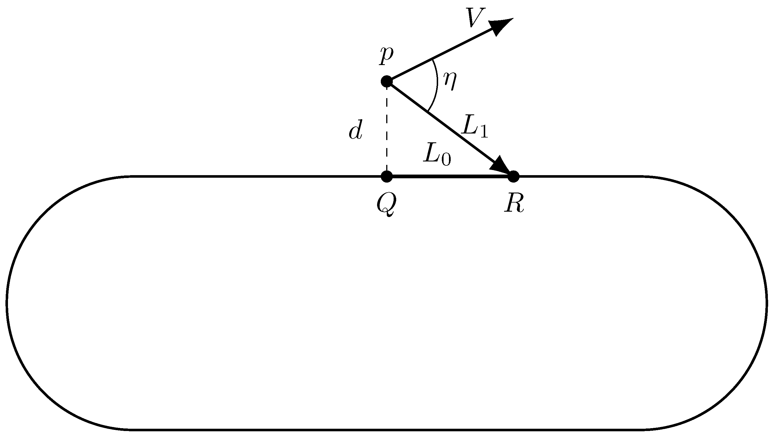
A modified version of the L1 controller that addresses the difficulties when the vehicle is far from the path is reported in [27]. We call such scheme the “L0 controller”. In the L0 controller, the parameter is no longer the design parameter to select, but rather, it is determined after selecting the new design parameter . The procedure is as follows. Firstly, the closest point to the vehicle in the path (Q) is computed, defining the cross-track error d. Then, a reference point is defined to be the point in the path that distances a given pre-defined jump from Q. Therefore, varies and it is equal to , being the controller design parameter. See Figure 5. This controller has been shown to be asymptotically stable and with a domain of attraction that is much larger than the domain of attraction of the L1 controller. In fact, it was shown that the L0 controller has a global domain of attraction even when the saturation of the actuators is considered (i.e., the stabilizing properties are valid in the same region where the dynamic model is considered valid).
Guidance Logic for AWES
Following both L1 and L0 guidance schemes presented before, the kite control acts on the roll angle in order to confer the lateral acceleration that is required to follow the path, i.e., the acceleration conferred to the kite computed in Equation (4) must be equal to the required centripetal acceleration of Equation (5). Then, solving for , we obtain an explicit expression for the reference roll angle:
Having a limited range for the values of the roll angle, , the guidance logic control with saturation is given by:
When the kite is far from the desired point, the controller can follow the path without additional approach logic (as is required in the case of L1 controller), with only the roll angle saturation.
In the simulations presented ahead, to model the fact that the roll angle cannot be changed instantaneously, we act on its time derivative using a proportional gain and taking into account the kite moment of inertia I around its longitudinal axis:
4. Simulation, Results, and Discussion
4.1. Kite and Flight Path Specification
The kite is set to follow a cyclic path on the surface of a sphere of radius r. The path is a closed curve parameterized in the space and can be of elliptical shape or figure-of-eight shape, for example. We have considered a closed curve, with similarities to an elliptical shape, divided by two curves and two straight lines in the space (see Figure 6).
This reference path has the parameters and , representing variations around the center of the curve . This curve in the space serves as a reference to be followed even when the tether length r varies. When projecting this reference path in the surface of the sphere, the path has four segments of constant curvature in the space. Finally, the roll angle limits imposed in the simulations are .
Figure 7 shows a 3D depiction of the trajectory of the kite over one of the simulations. The black line shows the kite position over time and allows us to observe the increasing tether length, while the red line shows the reference path projected onto a spherical surface with radius equal to the final tether length of the simulation and centered in the ground station.
4.2. Numerical Results
The dynamical model used in the simulations is the one described in Section 2.1 (see also [27,29]), and it was implemented in Simulink. We set the parameters of simulation for the AWES as in Table 1, which correspond to a small dimension prototype with a fixed angle of attack .
The initial conditions, as well as the results for each case of study, are presented in Table 2. The columns of the table are divided by the initial condition used for the simulation, the various sets of and values used (L is used when referring different sets of values) and finally the average (absolute) value, computed along time, of the cross-track error (d). The initial value of the simulations is defined in reference to the middle of the path curve .
There is one initial condition for each set of related and values. For each simulation, there are two values of : and . When and the kite is positioned exactly on the path, the reference point will be at the same distance for both L0 and L1 guidance schemes. When and the distance d from the kite to the closest point in the path Q is equal to , i.e., when , both the original and the resultant from the L0 controller will be equal, since the latter is computed as . These relations between the two parameters were chosen as they allow for an adequate comparison between methods, based on which we can retrieve quantitative performance measures such as the average value of the cross-track error.
The average value of the the cross-track error, , was computed for (including the initial transit behavior) and (steady-state error), and it is reported in Table 2. The latter was computed to better show the steady-state behavior of the cross-track error when there are large values of the error in the initial part. The minimum average error for each initial condition is highlighted in bold.
4.3. Performance Analysis
The results of the simulations are displayed in the next subsections, as well as with the Figure 8, Figure 9, Figure 10 and Figure 11. The results are organized for each set of . The figures present the kite position and the reference path in 2D, in a plane. Finally, an analysis using the cross-track error is performed in Section 4.3.5.
4.3.1.
In this case, the L value is small, compared with the other cases (see Figure 8). It forces the kite to have a sharp approximation to the path, which causes overshoot in various parts of the path. The kite is able to quickly decrease the distance to the path in the beginning by having a low L value. Low efficiency when following the path results in overshoot accumulation, with oscillating behavior around the path. In the case of , the kite loses track of the path and even inverts the flight direction. These L values result in a growth of the cross track error, mainly caused by the overshoots. Although this set of results is not the one that presents the worst error values, it presents qualitatively bad results for following the path, either when using the L1 controller or when using the L0 controller.
4.3.2.
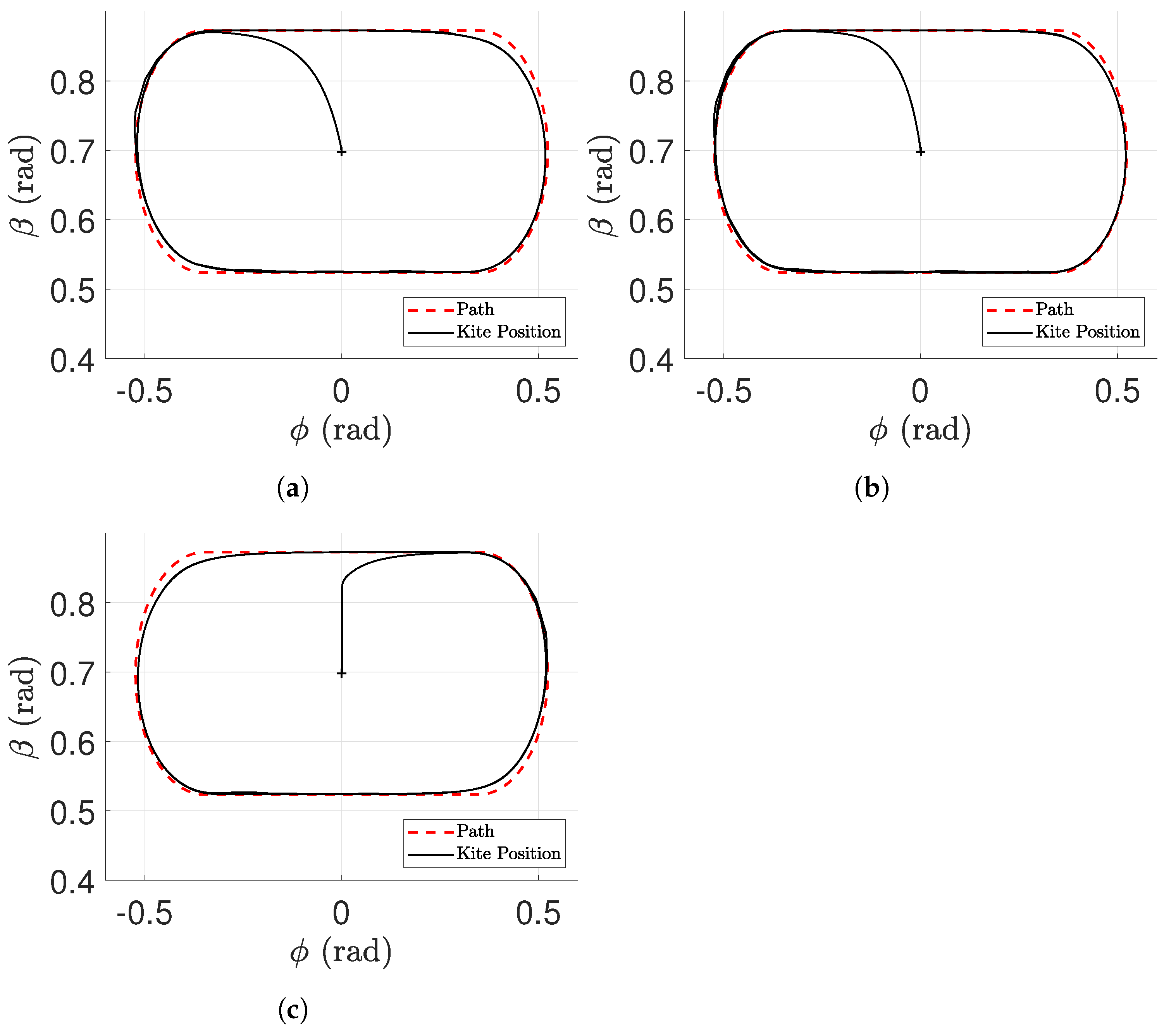
This set of results portrays the best performance overall, being the controller with the lowest cross-track error.
In Figure 9 it can be seen that, since the L1 controller only acts when the kite is close to the path and , the kite takes a sharper turn compared to the L0 controllers which start turning the kite as soon as the simulation starts. This behavior causes sharper turns than needed, which has as a consequence a larger required control actuation and can reduce the kite speed and thus cause a worse performance in terms of power production. Moreover, seems to feature a sharper turn during the initial approximation to the path than the case of , as expected due to its smaller parameter.
4.3.3.
In terms of the simulation error, the controller with has a smaller error than the others, thus being able to follow the path more closely (see Figure 10), as shown in Table 2.
Both and seem to have a small overshoot in the initial approximation to the path, being the former larger. This is due to the fact that the controller only begins to turn when and due to a smaller value of in the second case.
Overall these simulations remain showing fairly satisfying results with a small increase in error compared to the previous set of simulations .
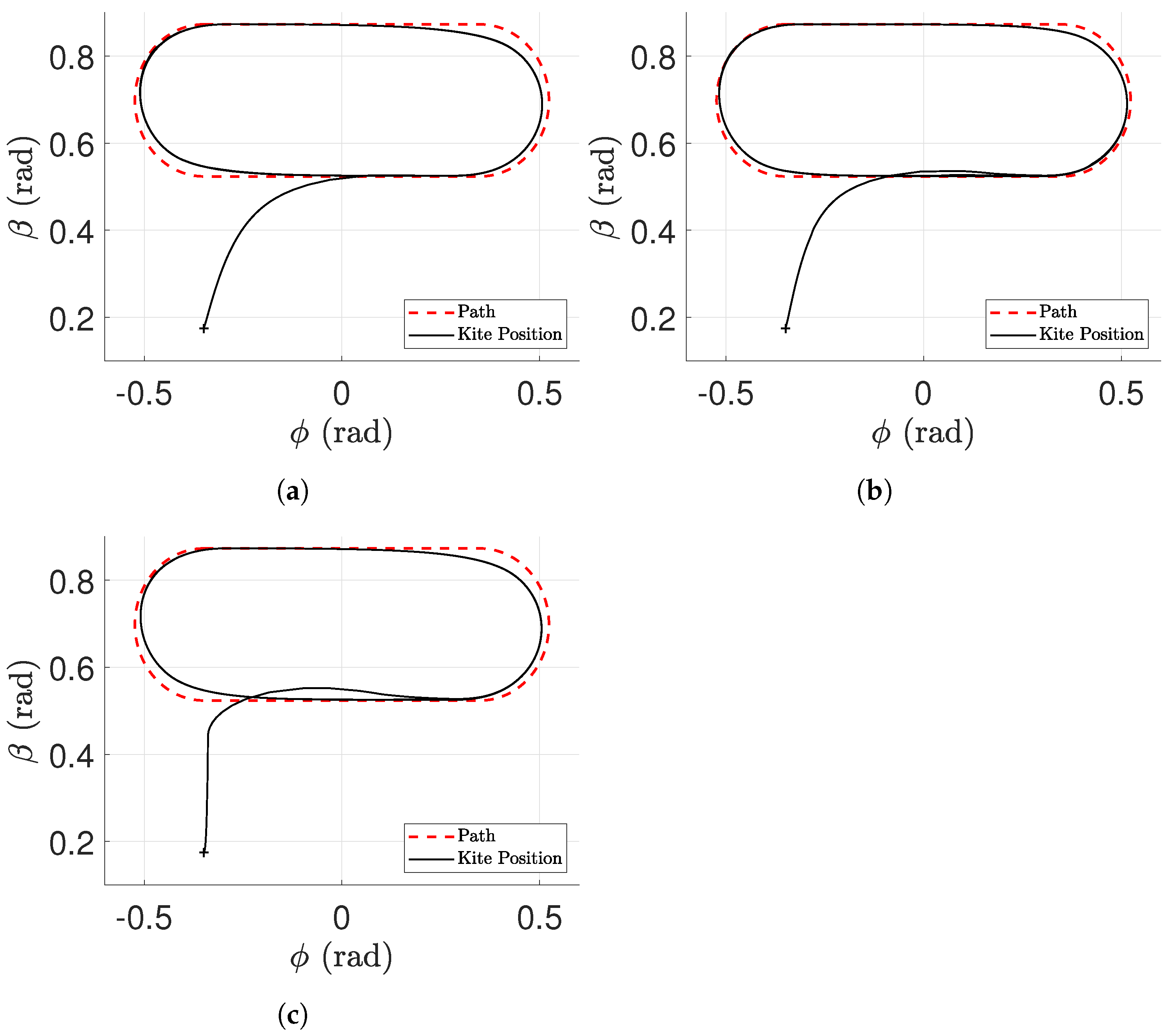
4.3.4.
This set of simulations shows the worst overall result in terms of error measurements, due to large L parameters. Therefore, the lowest L0 controller shows the best performance (see Figure 11). Since these parameters are too large, the controller picks up reference points that are far away from the current kite position which causes the kite to deviate from the path.
4.3.5. Cross-Track Error
Figure 12 shows two graphs portraying the evolution of the cross-track error between the kite’s current position and the closest point in the path over time. These are both from simulations taken from the L0 controller, one with and another with . The average cross-track error to the path over the full simulation is shown in red dotted lines, while the average cross-track error when the kite is already close to the path (steady-state error) is shown in a dotted black line. These graphs show that after an initial approximation to the path, the distance varies cyclically for both cases with a much larger amplitude in the second case, as expected due to its large parameter. Although this L0 controller was shown to be asymptotically stable in [27], it does not seem to converge to zero in these simulations. This happens since in [27] it is assumed a straight line as a path and not one with periodically varying curvature, as is the case with the path used in these simulations.
5. Conclusions
In this paper, we address the problem of controlling a kite (with fixed rigid wings) of an Airborne Wind Energy System (AWES) to follow a pre-determined path. We analyze, adapt to AWES, and implement two controllers: the widely used L1 guidance logic and a variant of it, which we named L0 guidance logic.
We compare the L1 and L0 guidance logics, with their application to AWES, carrying out both a qualitative and quantitative performance analysis. We considered the average of the absolute values of the cross-track error, computed along time, as a quantitative performance measure. The simulations with increasing L parameters show that for small values, the kite tends to overshoot and deviate from the path when there are larger curvatures. With larger values of L, the kite sets reference points in the path that are farther away from its current position, thus starting to respond earlier and resulting in a larger average distance from the path. Both guidance logics show similar performance overall: in some cases, the L0 controller shows a smaller cross-track error while in qualitative terms, the L1 controller shows sharper turns, since it only starts turning when . The sharper turns and an increased distance to the reference path might be reflected in lower power production performance for the AWES. The slightly better performance, combined with superior theoretical characteristics (larger domain of attraction for the controller and no need to switch control laws when far from the path), might make the L0 guidance logic the controller of choice in AWES.
In real application scenarios, the L parameters must be adjusted according to the wind speed. This is because their values can be considered too small or too large depending on the kite specifications and also its speed, which, in turn, is related with the existing wind conditions. The simulations in this work, however, were conducted with a fixed wind speed of m s−1. The simulation results show that the average cross-track error was an adequate performance measure. In future research, we aim to use this measure to alter the L parameters for varying wind conditions in order to adapt the controller in real time and search for the best possible performance.
Author Contributions
M.C.R.M.F. and S.V. had the major role in the literature review, software implementation, testing, validation and simulation of the concepts proposed; Conceptualization and methodology by M.C.R.M.F., L.T.P. and F.A.C.C.F.; Project administration and funding acquisition by F.A.C.C.F. All authors have contributed to the writing, reviewing and editing. All authors have read and agreed to the published version of the manuscript.
Funding
We acknowledge the support of COMPETE2020/FEDER/PT2020/POCI/MCTES/FCT funds, mainly through grant PTDC/EEI-AUT/31447/2017–UPWIND, but also grants PTDC/MAT-APL/28247/2017-ToChair, POCI-01-0145-FEDER-031821|FCT–FAST, and UID/EEA/00147/2019-SYSTEC.
Institutional Review Board Statement
Not applicable.
Informed Consent Statement
Not applicable.
Data Availability Statement
Not applicable.
Conflicts of Interest
The author declare no conflict of interest.
Nomenclature
| A | wing reference area of kite (m2) |
| tether reel-out acceleration (m s−2) | |
| kite lateral acceleration (m s−2) | |
| aerodynamic drag coefficient | |
| aerodynamic lift coefficient | |
| d | cross-track error (∘),(rad) |
| average cross-track error (∘), (rad) | |
| aerodynamic lift force (N) | |
| inertial forces (N) | |
| tether force (N) | |
| g | gravitational acceleration (m s−2) |
| distance ahead of the vehicle in the path (∘), (rad) | |
| distance ahead of the closest point to the vehicle in the path (∘), (rad) | |
| L | set of related values of and |
| m | mass (kg) |
| kite position (m) | |
| kite velocity (m s−1) | |
| Q | the closest point in the path to the vehicle |
| R | reference point in the path |
| r | tether length (m) |
| T | tether tension (N) |
| V | kite speed (m s−1) |
| apparent wind velocity (m s−1) | |
| tether reel-out speed (m s−1) | |
| wind velocity (m s−1) | |
| control vector | |
| state vector | |
| angle of attack (rad) | |
| azimuthal angle (rad) | |
| elevation angle (rad) | |
| roll angle (rad) | |
| angle between kite heading and heading to the reference target point (rad) | |
| air density (kg m−3) | |
| angle between kite velocity and path tangent (rad) |
References
- International Energy Agency. World Energy Outlook; Technical Report; International Energy Agency: Paris, France, 2021.
- Archer, C.L.; Caldeira, K. Global Assessment of High-Altitude Wind Power. Energies 2009, 2, 307–319. [Google Scholar] [CrossRef] [Green Version]
- Bechtle, P.; Schelbergen, M.; Schmehl, R.; Zillmann, U.; Watson, S. Airborne wind energy resource analysis. Renew. Energy 2019, 141, 1103–1116. [Google Scholar] [CrossRef]
- Vermillion, C.; Cobb, M.; Fagiano, L.; Leuthold, R.; Diehl, M.; Smith, R.; Wood, T.; Rapp, S.; Schmehl, R.; Olinger, D.; et al. Electricity in the Air: Insights From Two Decades of Advanced Control Research and Experimental Flight Testing of Airborne Wind Energy Systems. Annu. Rev. Control 2021. [Google Scholar] [CrossRef]
- European Union. Study on Challenges in the Commercialisation of Airborne Wind Energy Systems; Technical Report; Publications Office of the European Union: Brussels, Belgium, 2018.
- US Department of Energy. Report to Congress—Challenges and Opportunities for Airborne Wind Energy in the United States; Technical Report; US Department of Energy: Washington, DC, USA, 2021. [Google Scholar]
- Kitemill. Available online: https://www.kitemill.com/ (accessed on 5 January 2022).
- Ampyx Power. Available online: https://www.ampyxpower.com/ (accessed on 5 January 2022).
- TwingTec. Available online: https://twingtec.ch/ (accessed on 5 January 2022).
- UPWIND. The University of Porto Airborne WIND Energy Project. Available online: http://www.upwind.pt (accessed on 5 January 2022).
- Loyd, M.L. Crosswind kite power. J. Energy 1980, 4, 106–111. [Google Scholar] [CrossRef]
- Houska, B.; Diehl, M. Optimal control for power generating kites. In Proceedings of the 2007 European Control Conference (ECC), Kos, Greece, 2–5 July 2007; pp. 3560–3567. [Google Scholar] [CrossRef]
- Paiva, L.T.; Fontes, F.A. Mesh-Refinement Strategies for Fast Optimal Control and Model Predictive Control of Kite Power Systems. In Proceedings of the Airborne Wind Energy Conference 2015, Delft, The Netherlands, 15 June 2015. [Google Scholar]
- Paiva, L.T.; Fontes, F.A. Optimal Control Algorithms with Adaptive Time-Mesh Refinement for Kite Power Systems. Energies 2018, 11, 475. [Google Scholar] [CrossRef] [Green Version]
- Fernandes, M.C.R.M.; Paiva, L.T.; Fontes, F.A.C.C. Optimal Path and Path-Following Control in Airborne Wind Energy Systems. In Advances in Evolutionary and Deterministic Methods for Design, Optimization and Control in Engineering and Sciences; Springer International Publishing: Cham, Switzerland, 2021; pp. 409–421. [Google Scholar] [CrossRef]
- Cobb, M.K.; Barton, K.; Fathy, H.; Vermillion, C. Iterative Learning-Based Path Optimization for Repetitive Path Planning, With Application to 3-D Crosswind Flight of Airborne Wind Energy Systems. IEEE Trans. Control Syst. Technol. 2020, 28, 1447–1459. [Google Scholar] [CrossRef]
- Baheri, A.; Vermillion, C. Waypoint Optimization Using Bayesian Optimization: A Case Study in Airborne Wind Energy Systems. In Proceedings of the 2020 American Control Conference (ACC), Denver, CO, USA, 1–3 July 2020; pp. 5017–5102. [Google Scholar] [CrossRef]
- Aguiar, A.; Hespanha, J.; Kokotovic, P. Path-following for nonminimum phase systems removes performance limitations. IEEE Trans. Autom. Control 2005, 50, 234–239. [Google Scholar] [CrossRef] [Green Version]
- Fagiano, L.; Zgraggen, A.; Morari, M.; Khammash, M. Automatic Crosswind Flight of Tethered Wings for Airborne Wind Energy: Modeling, Control Design, and Experimental Results. IEEE Trans. Control Syst. Technol. 2013, 22, 1433–1447. [Google Scholar] [CrossRef] [Green Version]
- Erhard, M.; Strauch, H. Flight control of tethered kites in autonomous pumping cycles for airborne wind energy. Control Eng. Pract. 2015, 40, 13–26. [Google Scholar] [CrossRef] [Green Version]
- Rontsis, N.; Costello, S.; Lymperopoulos, I.; Jones, C. Improved path following for kites with input delay compensation. In Proceedings of the 2015 54th IEEE Conference on Decision and Control (CDC), Osaka, Japan, 15–18 December 2015; pp. 656–663. [Google Scholar] [CrossRef] [Green Version]
- Rapp, S.; Schmehl, R.; Oland, E.; Smidt, S.; Haas, T.; Meyers, J. A Modular Control Architecture for Airborne Wind Energy Systems. In Proceedings of the AWESCO, Shenzhen, China, 1–2 July 2019. [Google Scholar] [CrossRef] [Green Version]
- Uppal, A.A.; Fernandes, M.C.R.M.; Vinha, S.; Fontes, F.A.C.C. Cascade Control of the Ground Station Module of an Airborne Wind Energy System. Energies 2021, 14, 8337. [Google Scholar] [CrossRef]
- Lellis, M.D.; Saraiva, R.; Trofino, A. Turning angle control of power kites for wind energy. In Proceedings of the 52nd IEEE Conference on Decision and Control, Firenze, Italy, 10–13 December 2013; pp. 3493–3498. [Google Scholar] [CrossRef]
- De Lellis, M.; Saraiva, R.; Trofino, A. Optimization of Pumping Cycles for Power Kites. In Airborne Wind Energy: Advances in Technology Development and Research; Schmehl, R., Ed.; Green Energy and Technology; Springer: Singapore, 2018; pp. 335–359. [Google Scholar] [CrossRef]
- Park, S.; Deyst, J.; How, J. A New Nonlinear Guidance Logic for Trajectory Tracking. In Proceedings of the AIAA Guidance, Navigation, and Control Conference and Exhibit, Providence, RI, USA, 16–19 August 2004. [Google Scholar] [CrossRef] [Green Version]
- Silva, G.B.; Paiva, L.T.; Fontes, F.A. A Path-following Guidance Method for Airborne Wind Energy Systems with Large Domain of Attraction. In Proceedings of the 2019 American Control Conference (ACC), Philadelphia, PA, USA, 10–12 July 2019; pp. 2771–2776. [Google Scholar]
- Fernandes, M.C.R.M.; Silva, G.B.; Paiva, L.T.; Fontes, F.A.C.C. A Trajectory Controller for Kite Power Systems with Wind Gust Handling Capabilities. In Proceedings of the 15th International Conference on Informatics in Control, Automation and Robotics, Porto, Portugal, 29–31 July 2018; pp. 533–540. [Google Scholar]
- Fernandes, M.C.R.d.M. Airborne Wind Energy Systems: Modelling, Simulation and Economic Analysis. Master’s Thesis, Universidade do Porto, Porto, Portugal, 2018. [Google Scholar]
- Bechtle, P.; Gehrmann, T.; Sieg, C.; Zillmann, U. AWEsome: An open-source test platform for airborne wind energy systems. arXiv 2017, arXiv:1704.08695. [Google Scholar]
- ArduPilot. Navigation Tuning—Plane Documentation. 2021. Available online: https://ardupilot.org/plane/docs/navigation-tuning.html (accessed on 10 February 2021).
- Plane: L1 Control for Straight and Curved Path Following by brnjones · Pull Request #101 · ArduPilot/Ardupilot. Available online: https://github.com/ArduPilot/ardupilot/pull/101 (accessed on 20 February 2021).
Figure 1.
Global and Local Coordinate Systems representation.

Figure 2.
Roll angle and turning dynamics.

Figure 3.
Path-following model coordinates .

Figure 4.
Guidance logic schematic [26].
Figure 4.
Guidance logic schematic [26].

Figure 5.
L1 and L0 guidance logic scheme.

Figure 6.
Kite path specification.

Figure 7.
3D kite trajectory.

Figure 8.
, . (a) , (b) , (c) .

Figure 9.
, . (a) , (b) , (c) .

Figure 10.
, . (a) , (b) , (c) .

Figure 11.
. (a) , (b) , (c) .

Figure 12.
Cross-Track Error—d. (a) , (b) .


Table 1.
Simulation parameters.
| Parameter | Value |
|---|---|
| 1.2 kg m−3 | |
| 10 m s−1 | |
| g | 9.8 m s−2 |
| m | 0.7 kg |
| A | 0.28 m2 |
| 3.33 m s−1 | |
| 0.112 | |
| 1.3 |
Table 2.
Parameters used in the simulations.
| L | |||
|---|---|---|---|
| 0.0078 | 0.0039 | ||
| ()° | 0.0089 | 0.0052 | |
| 0.0157 | 0.0125 | ||
| 0.0123 | 0.0044 | ||
| ()° | 0.0124 | 0.0043 | |
| 0.0108 | 0.0027 | ||
| 0.0253 | 0.0111 | ||
| 0.0250 | 0.0105 | ||
| 0.0208 | 0.0062 | ||
| 0.0460 | 0.0441 | ||
| 0.0399 | 0.0383 | ||
| 0.0228 | 0.0197 |
Publisher’s Note: MDPI stays neutral with regard to jurisdictional claims in published maps and institutional affiliations. |
© 2022 by the authors. Licensee MDPI, Basel, Switzerland. This article is an open access article distributed under the terms and conditions of the Creative Commons Attribution (CC BY) license (https://creativecommons.org/licenses/by/4.0/).
Share and Cite
MDPI and ACS Style
Fernandes, M.C.R.M.; Vinha, S.; Paiva, L.T.; Fontes, F.A.C.C. L0 and L1 Guidance and Path-Following Control for Airborne Wind Energy Systems. Energies 2022, 15, 1390. https://0-doi-org.brum.beds.ac.uk/10.3390/en15041390
AMA Style
Fernandes MCRM, Vinha S, Paiva LT, Fontes FACC. L0 and L1 Guidance and Path-Following Control for Airborne Wind Energy Systems. Energies. 2022; 15(4):1390. https://0-doi-org.brum.beds.ac.uk/10.3390/en15041390
Chicago/Turabian StyleFernandes, Manuel C. R. M., Sérgio Vinha, Luís Tiago Paiva, and Fernando A. C. C. Fontes. 2022. "L0 and L1 Guidance and Path-Following Control for Airborne Wind Energy Systems" Energies 15, no. 4: 1390. https://0-doi-org.brum.beds.ac.uk/10.3390/en15041390
Note that from the first issue of 2016, this journal uses article numbers instead of page numbers. See further details here.