Numerical Evaluation of the Effect of Fuel Blending with CO₂ and H₂ on the Very Early Corona-Discharge Behavior in Spark Ignited Engines

Abstract

Reducing green-house gases emission from light-duty vehicles is compulsory in order to slow down the climate change. The application of High Frequency Ignition systems based on the Corona discharge effect has shown the potential to extend the dilution limit of engine operating conditions promoting lower temperatures and faster combustion events, thus, higher thermal and indicating efficiency. Furthermore, predicting the behavior of Corona ignition devices against new sustainable fuel blends, including renewable hydrogen and biogas, is crucial in order to deal with the short-intermediate term fleet electric transition. The numerical evaluation of Corona-induced discharge radius and radical species under those conditions can be helpful in order to capture local effects that could be reached only with complex and expensive optical investigations. Using an extended version of the Corona one-dimensional code previously published by the present authors, the simulation of pure methane and different methane–hydrogen blends, and biogas–hydrogen blends mixed with air was performed. Each mixture was simulated both for 10% recirculated exhaust gas dilution and for its corresponding dilute upper limit, which was estimated by means of chemical kinetics simulations integrated with a custom misfire detection criterion.

1. Introduction

Advances in the internal combustion engines design are necessary in order to effectively reduce the carbon dioxide tailpipe emissions while carbon-free technologies for light duty vehicles become mature. With regard to Spark Ignition (SI) engines, two of the main limiting factors against the improvement of fuel economy are the pressure losses during throttled operations, and the very high cycle average temperature compared with that of Compression Ignition (CI) engines, which strongly affect the indicating and the thermal efficiency, respectively. A promising solution to approach those issue is using a high amount of Exhaust Gas Recirculation (EGR) in order to dilute the fresh charge, thus allowing for the cylinder empty-filling at low load with reduced throttling at the intake manifold and the reactive gas to cool down (lower heat losses and knock mitigation) [1,2]. One of the main concerns regarding highly diluted operations is the flame stability, together with the risk of incomplete combustion and ignition failure [3,4]. Therefore, in order to run engine operations richer in EGR while ensuring combustion stability and repeatability, the use of supporting device is compulsory. In this framework, the equipment of the engine with High Frequency Ignition (HFI) spark devices based on the so-called Corona discharge effect [5,6] has proven to be a powerful solution to boost combustion stability and velocity. In [7], Pienda et al. compared classical and Corona spark devices in a research engine implementing a wide Design Of Experiments (DOE). When observing the indicating data, the authors reported that at low speed-low load conditions the Corona discharge is able to speed up combustion, improving diluted operations at given EGR. At moderate speed-high load (turbocharger active), the use of Corona discharge has shown also the ability to extend the engine knock limit. Furthermore, the HFI system allows for a general reduced fuel consumption with respect to the classical spark because of the larger combustion volume. In [8], Marko et al. conducted experiments on an optical accessible engine fueled with methane at stoichiometric conditions emphasizing the influence of the ignition system (Corona or classical spark) on the EGR limit. The authors showed that for both the ignition devices the Coefficient Of Variation (COV) of the engine Indicating Mean Effective Pressure (IMEP) has a steep abrupt increase with respect to EGR, highlighting the existence of an EGR dilution threshold value regardless of the ignition system. However, the experimental results show that the use of the Corona ignition can delay the EGR threshold value from 27% to 32%. Furthermore, reduced standard deviation were reported for both the occurrence of the 50% Mass Fuel Burned (MFB50) and kernel formation at given EGR in the case of Corona ignition. Other relevant literature findings also report the potential of the Corona ignition device as lean limit extender to promote the stabilization of combustion events at very low equivalence ratio ($\varphi$, fuel–air ratio normalized against stoichiometric) [9,10,11,12]. Considering the high attention gained by the use of renewable hydrogen in fuel blends for the next on-road transportation, the exploration of technological solutions to support the ignition of such molecule is of primary interest. Indeed, despite the fact that hydrogen can enhance efficient low load operations at unthrottled conditions due to its larger flammability limit [13,14], there are concerns on its behavior at high loads due to its characteristic very low ignition energy, which results in unacceptable pre-ignition events [13,14]. Since the hydrogen ignition energy is a $\varphi$-dependent steep decreasing function, ignition systems capable of operating reliable ignitions in ultra-lean environment such as Corona devices are compulsory. In this respect, in [9] Cruccolini et al. have published the results of experiments on an optical research engine with port fuel feeding of pure methane, pure hydrogen, and a methane–hydrogen mixture, which were ignited with both classical spark and Corona devices. The authors reported that the advantage of equipping the engine with Corona systems is weaker if hydrogen is concerned with respect to hydrocarbons (gasoline, methane). However, it was detected that the combination of hydrogen fuel and Corona ignition leads to a slight extension of the lean limit of classical ignition systems ($\varphi$ 0.5 vs. 0.52, respectively) and shorter combustion duration. In light of what described on the effect of Corona discharge on ignitable mixtures including significant amount of hydrogen and carbon dioxide, the characterization of Corona-induced ignition at engine relevant conditions can be crucial also to assess the very early ignition behavior of biogas (CH₄ + CO₂)-hydrogen blends in SI engines, in which hydrogen play the role of booster of the combustion properties and mixture dilution limit as reported in [13,14,15,16,17,18,19,20].

This work deals with the use of an in-house developed one-dimensional model for the steady state simulation of Corona discharge able to predict the initial discharge radius and the spatial distribution of the discharge-induced radical species, which was tested on mixtures consistent with next low-carbon fuel blends. The code was presented and discussed in a previous work of the present authors [21]. The additional contribution of this work lies in the fact that the chemical kinetics core integrated in the model was improved to address the simulation of renewable fuel mixtures in CO₂-rich environment. Methane was considered as benchmark, then, different blending with H₂, CO₂, and H₂-CO₂ were tested to represent the effect of adopting hydrogen and biogas. The behavior of the discharge on each mixture is evaluated at fixed dilution with EGR 10%wt as well as at the maximum stable dilution with EGR, which was different for each test mixture. Those upper EGR threshold values were estimated by means of a simplified energetic criterion based on the kernel energy needed to stabilize the combustion after ignition occurs. The latter is proportional to the fuel consumption rate, equal to the adiabatic laminar flame speed, reached inside the kernel, function of thermodynamics conditions and composition. A Gaussian process regressor fitted on laminar flame speed values obtained with detailed chemical kinetics simulations has been adopted for evaluating eight test mixtures with increasing EGR from 10% to 44% by step of 2%.

2. Methodology

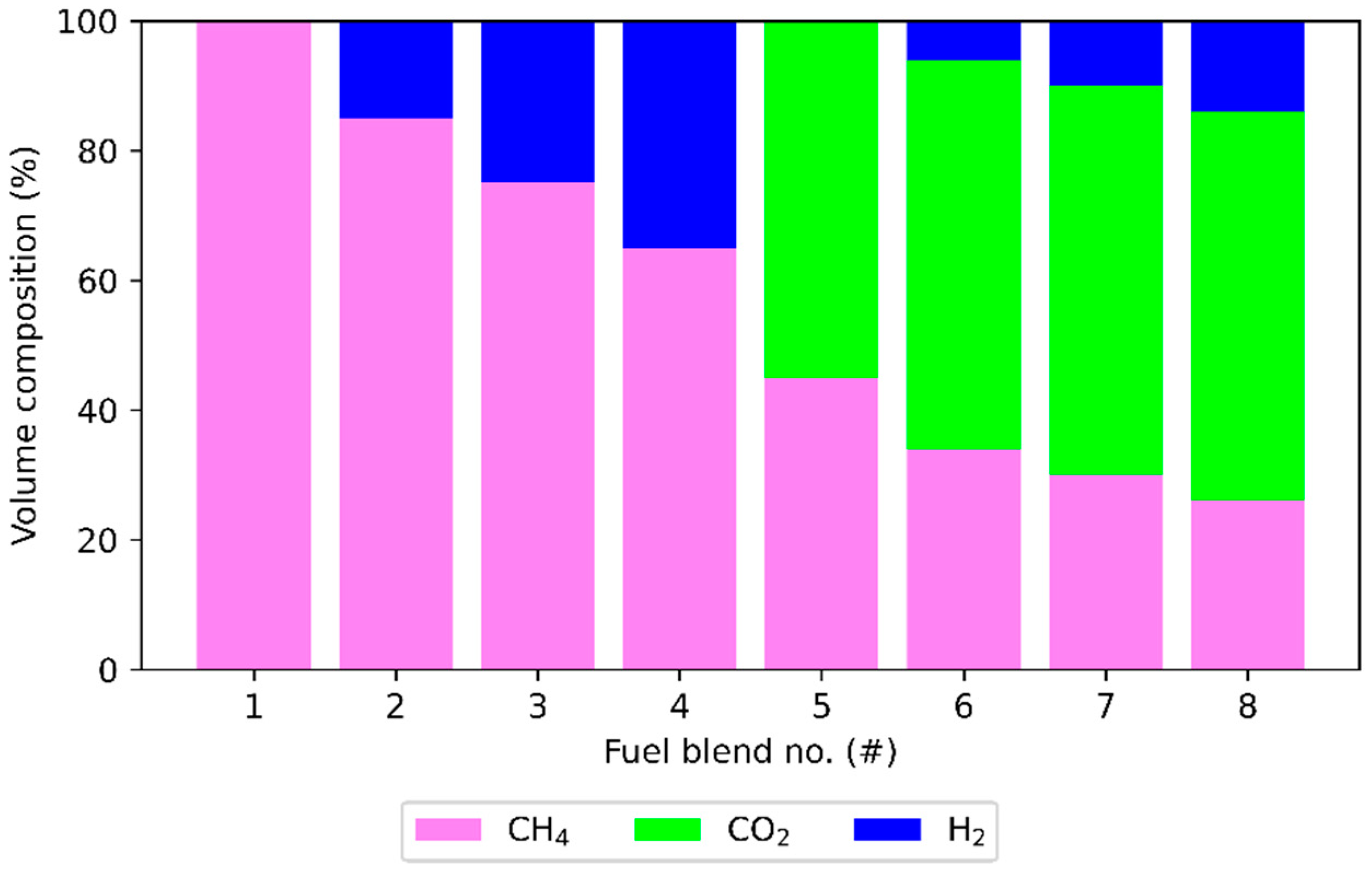
2.1. Test Mixtures

Simulations were run considering eight different test fuels whose composition was set based on literature findings on biogas composition [17,18,19,20,22] and hydrogen blending [9]. The composition of each fuel is shown in Figure 1: fuel no. 1 is pure methane, which was considered to set a benchmark; blends from no. 2 to no. 4 are methane–hydrogen blends; blends from no. 5 to no. 8 are different compositions of biogas characterized by the presence of carbon dioxide.

2.2. Reference Engine Thermodynamic Model

As far as the solution of the plasma physics is concerned, the gas conditions (temperature, density) at which the Corona discharge is simulated are necessary. Therefore, a zero-dimensional engine simulation approach was used in order to determine gas conditions representative of the in-cylinder engine environment during compression stroke. The Diesel power unit-based engine equipped with a Corona tip and operated with SI methane described in [8] was considered as a reference. The main engine data are reported in

Table 1. Main specifications of the reference SI engine from [8].

Engine Geometry
no. Cylinder	1
Displacement	2.47 L
Bore (mm)	139 mm
Stroke (mm)	163 mm
Stroke-Bore ratio (#)	1.17
Compression ratio (#)	13:1
Engine speed (r/min)	1100

. Once the engine was identified, the combustion chamber internal energy balance (Equation (1)) was solved for the gas temperature (T) with the Euler forward method together with the perfect gas law (Equation (2)) for the pressure (P). In Equation (1) $m_{trap}$ is the gaseous mass (air + fuel blend + exhausts) trapped in the cylinder after the intake valve closing, $c_V$ is the gas specific heat at constant volume, $V_C$ is the instantaneous engine displacement volume, $Q_W$ is the energy contribution due to heat losses at the engine walls (head, piston, and cylinder wall were accounted for), R is the mixture gas constant, and $\theta$ is the time variable in crank angle degrees.

It is underlined that in Equation (1) the positive energy contribution due to combustion is not taken into account since the engine thermodynamics simulation was run up to the spark timing. The wall heat losses were modeled according to the widely adopted Woschni’s convective formulation [23], which was tuned by a scaling coefficient in order to capture the in-cylinder pressure curve presented in [8] up to the ignition timing.

$$m_{trap}{c}_V\frac{d T}{d\theta }=-P\frac{d V_C}{d\theta }+\frac{d Q_W}{d\theta }$$

(1)

$$P=\frac{m_{trap} R T}{V_C}$$

(2)

The presented gas conditions and compositions were included in a simulation matrix aimed at evaluating the effect of the charge dilution with EGR. Firstly, the gaseous composition of the fresh mixture for each fuel blend is calculated considering that since the influence of carbon atoms can be neglected as described in Section 1, methane behaves as hydrogen molecules (2H₂). Thus, for methane–hydrogen blends and biogas–hydrogen blends, methane is cumulated in hydrogen during the molar fraction calculation. The presence of oxygen and nitrogen is calculated considering the operated air fuel ratio. In this work, lean operations characterized by $\varphi$ = 0.57 − 0.65 were simulated. Then, compositions were updated by including water vapor, additional carbon dioxide and nitrogen representing EGR, then the molar fractions were re-normalized based on the EGR amount added. It must be underlined that for the reference engine conditions [8], the fuel is provided via external gas injection towards the intake manifold. As a consequence, in spite of the relevance of design factors such as the charge vortex motion intensity (swirl in this case) and the piston bowl shape on the mixture distribution, it was assumed that the use of the nominal mixture compositions is a sufficient representation of the tip local distribution, since considering the present fueling system (no fuel spray direct injection, no wall film), a premixed monophasic uniform mixture should be promoted. Furthermore, it was assumed that the characteristic time scales of the fluid flow are significantly larger than that required to establish the discharge volume with Corona device (1–10 ns). Thus, the species time evolution in this interval due to the vortex-induced mixing was considered negligible with respect to that promoted by the species mutual interactions (chemical kinetics scales) and the species-electrons interactions (electronic collisions scales).

For the sake of comparison, two very different EGR configurations were simulated and discussed: (i) low EGR, in which a fixed amount of 10% EGR is operated, so the charge dilution relies mainly on the lean conditions; (ii) high EGR, in which the exhausts (additional N₂, additional CO₂, H₂O) play a key role in the charge dilution as that of the air excess. It must be considered that the identification of a single value for the high EGR was not viable because relatively high dilution level for methane–hydrogen blends (e.g., around 30% thanks to the presence of hydrogen) is not applicable to biogas mixtures, which are not able to ignite at those EGR also due to the significant presence of CO₂. Therefore, in order to perform a fair comparison, the high EGR configuration of each fuel blend was identified as that corresponding to the higher EGR quantity at which the test fuel burns under stable conditions, i.e., no misfire occurs.

2.3. Maximum Stable EGR Definition by Detailed Chemical Kinetics

In order to identify the mean energy of the initial flame kernel following the hypothesis of the flamelet method, it is necessary to compute the reaction speed of the combustible mixture, the surface of the kernel and the available energy provided by the fuel (i.e., fuel mass times the LHV (Lower Heating Value)). The reaction speed of a mixture characterized by a given composition and pressure–temperature conditions can be computed by resolving a steady planar and adiabatic laminar flame, where the consumption speed, by definition, equals the displacement speed obtained at the domain inlet. To perform these simulations for all the considered conditions, the chemical kinetics library Cantera was used, and a one-dimensional domain with successive refinement was resolved, following the strategy described in [24] for the solution procedure and domain length identification. The chemical kinetics scheme adopted was derived from the NUIGMech 1.1 kinetics scheme [25] developed by the Combustion Chemistry Center NUI Galway, by automatically removing all the species and reactions that were not involved in CH₄ or H₂ pathways, leading to a final mechanism comprising of 40 species and 217 reactions that could be resolved, on average, in 4.7 min on a CPU Intel i7 7700 with 16GB RAM. The validation of the reduced mechanism is shown in Figure 2 for two different conditions (ambient, and P = 10 bar, T = 580 K) against experimental data [26] recorded for the combustion of pure methane and methane-hydrogen in air. Figure 2 displays that the laminar flame speed simulation with the proposed mechanism (lines) is in nice agreement with experimental data (markers), especially considering the lean-branch of the bell-shaped curves (x-axis left-hand side), which is the range of interest for this application.

Based on the above-mentioned reduced mechanism, laminar flame simulations involving the additional presence of inert gases (N₂, CO₂, H₂O) in quantities corresponding to EGR dilution levels from 10% to 44% should be performed in order to detect the limiting EGR value for each of the eight fuel blends. In order to allow for a more rapid evaluation of the laminar flame speed during the successive calculations, a regression algorithm has been developed and trained on the available dataset. After internal evaluations regarding different algorithms, the Gaussian Process regressor with the classic radial basis function prior was selected for its capacity to interpolate exactly the known values and prediction of the confidence interval and given the limited size of the available dataset (155 points in total). The machine learning workflow adopted consisted in: (i) split of the dataset into train and test set with an 80/20 ratio, to evaluate the accuracy of the algorithm on unseen points; (ii) definition of the minimum and maximum values of the train dataset to scale the input data between 0 and 1; and (iii) train of the regression algorithm on the scaled train set and evaluation of the performance on both train and test set. The overall performance, measured by means of the R² (coefficient of determination) value was considered appropriate for this application (R² > 0.991 for both train and test set) without the need for significant optimization effort on the hyperparameters of the model that were left to the default values prescribed in the Scikit-learn open library employed [27], apart from the alpha value, increased to 1 × 10⁻⁵ to prevent overfitting and the choice to scale the target data during training.

Once the algorithm was implemented, a reference initial discharge radius was needed to calculate the kernel volume, furthermore, a lower threshold value of the kernel energy that must be achieved was defined. The reference discharge radius was set to 5 mm according to different experimental data on Corona ignition from the literature [9,10,11]. The minimum energy that must lie in the kernel in order to generate a stable ignition was estimated based on a simplified criterion based on the experimental evidence reported in the experimental reference case [8] for the Corona ignition of methane. Firstly, it was considered that as shown in [8] the Corona ignition of a stoichiometric air–methane mixture in the reference engine can be stably operated with EGR up to 32%, after this value the COV of the IMEP performance index has a steep rise above 2%, which is usually considered the confidence limit in engine experiments. Therefore, assuming a uniform distribution of the mixture around the Corona tip, one can express the minimum energy that must be developed at the ignition time as in Equation (3), in which LHV is 50 MJ/kg for methane, and M_F32 is the fuel mass that is present downstream the Corona tip at the reference stability limiting conditions, i.e., $\varphi$ = 1, EGR = 32%. The latter can be computed as shown in Equation (4), in which w_F32 is the methane mass fraction at the reference stability limiting conditions, ρ is the gas density during compression stroke at the ignition timing. The other terms represent the discharge volume assumed as a sphere of radius equal to the abovementioned reference discharge radius R_D. w_F32 was calculated by means of the in-cylinder mass balance between air, fuel, and EGR considering the air–methane stoichiometric mass ratio (17.2) and the limiting EGR (32% of the trapped air). The gas density was calculated by means of the perfect gas law considering the pressure and the temperature values given by Equations (1) and (2). As a result, a minimum kernel energy of around 600 mJ was defined as the lower energy bound for this case.

$$E_{k,MIN}=M_{F32} LHV$$

(3)

$$M_{F32}=w_{F32} \rho \frac{4}{3}\pi R_D^3$$

(4)

2.4. Corona-Discharge Model

The current paper aims to extend the previous work by the same authors [21] on the characterization of radical species production from Corona discharge generated by a one-tip HFI device under engine-like environmental conditions. In the previous work, a reduced chemical kinetics set accounting for H₂, N₂, and O₂, representing fuel and air, was considered. It is important to remember that interactions involving carbon atoms were neglected because in this type of phenomenon, oxidation events of hydrocarbon molecules are overwhelmed by dissociation reactions that follow a photo-excitation process, acting on a smaller time scale than enthalpy-driven reactions. Therefore, they have a small impact on the cumulative reaction rate of the species. In this work, a more detailed model is proposed implementing the contributions of H₂O, CO₂, and CO species. Furthermore, the extended version of the solver is now focused on the perspective to test conditions richer in air and CO₂, representative of fuel blends comprising biogas and hydrogen. It is underlined that only the pre-flame very early discharge behavior is studied, including observations on the initial discharge volume, while the effects of the follow up combustion event is not taken into consideration. As a result, the code is able to compute the initial discharge radius and every species’ spatial concentration distribution, considering radical recombination given by the additional species.

For the sake of clarity, the complete workflow of the Corona ignition model is schematically represented in Figure 3 with the flow-chart of the algorithm. The code relies on three steps: (i) feeding with swarm transport thermodynamic and electric conditions the electron transport equation for electrons, positive ions and negative ions, coupled with the charge conservation equation; (ii) the Boltzmann equation, which computes the EEDF (Electron Energy Distribution Function) and collision rates based on cross sections data and operative conditions; and (iii) the extended chemical kernel. The whole process exits from the loop when convergence occurs. Convergence is assumed to be reached when the composition update absolute error is less than the absolute tolerance of 1 × 10⁻⁶.

The computational grid is a one-dimensional domain in spherical coordinates, with polar and azimuthal symmetry. Along the radial coordinate, the domain is bounded by the tip of the HFI plug device on the one side, and the piston crown on the other side, which is considered as the grounded surface. The grid independence test, which has already been performed in [21], revealed that the species distribution produced by adopting the typical size used in CFD simulations in the spark plug proximity for classical ignition simulation (around 0.1–0.15 mm) were slightly different from those achieved with grid element size in the range 0.01–0.005 mm, which instead have shown almost overlap results. As a consequence, the size of each element promoting mesh convergence while accurately capturing radial variation of the molar fractions was set to 40 µm with a uniform distribution. For the punctual description of the features of the preexisting physical model, the interested reader can refer to [21].

2.4.1. Electron Transport

Considering polar and azimuthal symmetry, transport equation can be rewritten for electrons, positive and negative ions as in Equations (5)–(8), in which subscripts e, p, n refers to electrons, positive ions and negative ions, respectively. $n$ is the number density (${\mathrm{m}}^{-3}$); $\mu$ is the mobility coefficient (${\mathrm{m}}^2{\mathrm{V}}^{-1}{\mathrm{s}}^{-1}$); $D$ is the diffusion coefficient (${\mathrm{m}}^2{\mathrm{s}}^{-1}$); $\alpha$ is the ionization coefficient (${\mathrm{m}}^{-1}$); $\beta$ is the attachment coefficient (${\mathrm{m}}^{-1}$); ${\beta }_{ep}$ is the recombination coefficient for positive ions and electrons (${\mathrm{m}}^3{\mathrm{s}}^{-1}$); and ${\beta }_{np}$ that for positive and negative ions (${\mathrm{m}}^3{\mathrm{s}}^{-1}$). The electric field is E (V/m), whilst the electric potential electric is $V$ ($\mathrm{V}$), ${ϵ}_0$ is the vacuum permittivity ($\mathrm{F}{\mathrm{m}}^{-1}$), the electron charge is defined with $e$ ($\mathrm{C}$). Finally, the source term $S_{ph}$ describes the photo-ionization effect.

$$\nabla ·\left(D_e\nabla \left(n_e\right)\right)+\nabla ·\left(n_e {\mu }_e E\right)+{\beta }_{ep} n_p n_e-S_{ph}=-\left(\alpha -\beta \right) n_e {\mu }_e E$$

(5)

$$\nabla ·\left(n_p{\mu }_{p}E\right)+{\beta }_{ep}{n}_p{n}_e=\alpha n_e{\mu }_{e}E+S_{ph}$$

(6)

$$\nabla ·\left(n_n{\mu }_{n}E\right)+{\beta }_{np}{n}_n{n}_p=-\beta n_e{\mu }_{e}E$$

(7)

$${\nabla }^{2}V=-e \left(n_p-n_n-n_e\right)/{ϵ}_0$$

(8)

The numerical solution of Equations (5)–(8) is initialized by solving Equation (8) as for a Laplacian field (right hand side equal to zero) and using the theoretical relationship $E=-\nabla V$ to determine the associated initial electric field, which is then used to calculate the initial number density values of charged species according to the system composed of Equations (5)–(7). Once the number density values are calculated, the complete form of Equation (8) is solved.

2.4.2. Boltzmann Equation

The formulation of the Boltzmann equation for electrons and ionized gas is based on the assumption that inside a non-equilibrium plasma, e.g., Corona discharge and electrons elastic collision are mainly promoted. Considering the small inertia of electrons, the energy loss given by their collision is negligible if compared with that of heavier species. Therefore, the mean thermal speed can be considered as the most influencing property, thus, the electron distribution is considered isotropic. As a result, the Boltzmann steady-state equation for EEDF can be rewritten as in Equation (9), in which $f_0$ is the EEDF, $M_h,m_e$ are the mass of electrons and heavier species ($\mathrm{kg}$), respectively. u is the electrons kinetic energy ($\mathrm{eV}$), ${\nu }_m$ is the electron elastic collision frequency (${\mathrm{m}}^3{\mathrm{s}}^{-1}$), and $Q\left(f_0\right)$ is the inelastic integral (${\mathrm{m}}^3\mathrm{k}{\mathrm{g}}^{-1}{\mathrm{s}}^{-1}$). The latter is computed as a sum of four contributions, namely excitation, dissociation, attachment and ionization. The values of the collision frequency were calculated by means of the associated cross sections determined via the LxCat database [28], which must be provided with the gas density and temperature, and the nature and concentration of the species involved in collisions.

$$\frac{2 e}{3 m_e}\frac{d}{du}\left(\frac{u^{3/2}E{ }^2}{{\nu }_m}\frac{d{f}_0}{du}+\frac{3 m_e^{ } u^{3/2} {\nu }_m f_0}{e M_h}\right)+u^{1/2}Q\left(f_0\right)=0$$

(9)

Once the Boltzmann solver has returned the EEDF, the reaction rate $R_{ij}$ of the j-th species interacting with electrons according to the i-th mechanism (excitation, dissociation, attachment, or ionization) was defined as in Equation (10). For the sake of illustration, the EEDF returned by the Boltzmann solver based on the temperature-density-composition data provided by the engine thermodynamics model is shown in Figure 4 for the case one (reference, pure methane). It is visible that at the HFI tip (radius equal to zero) there is an almost equiprobable distribution of the energies in the visible spectra that electrons may have. Then, the longer is the distance from the tip, the more the electrons’ energy is distributed over the lower values (5–20 eV) due to the electric filed magnitude derating. Those results are in line with the evidence shown in [29]. The Boltzmann solver validation has already been performed in the previous work [21], with comparison between the implemented in-house solver and two different open software options. The procedure also compared total ionization and attachment collision rates showing good matching of the results.

$$R_{ij}=x_j{n}_h{n}_e\gamma {{\displaystyle \int }}_0^{u_f}u{\sigma }_{ij}{f}_{0}du, \gamma ={\left(2e/m_e\right)}^{1/2}$$

(10)

2.4.3. Extended Chemical Kernel

In order to describe the kinetic behavior of each reaction, a classical Arrhenius model is assumed, comprehensive of the additional species integrated in this work. In addition to both the radical and molecular forms of nitrogen, oxygen and hydrogen, water vapor (H₂O), carbon dioxide (CO₂), and monoxide (CO) are now considered. The corresponding additional reactions, each one with its kinetic constant k (which is temperature dependent), are expressed by:

• CO + O → CO₂
• H + OH → H₂O

Both can be schematized with a classical kinetic law, leading to the usual definition of recombination rates as in Equations (11) and (12), in which C is the species concentration (mol/m³). Then, the solving equation in steady state regime for the generic species was approached according to the Equation (25) reported in [21].

$$R_{{\mathrm{CO}}_2,chem}=k_{{\mathrm{CO}}_2} C_{\mathrm{CO}} C_{\mathrm{O}}$$

(11)

$$R_{{\mathrm{H}}_2\mathrm{O},chem}=k_{{\mathrm{H}}_2\mathrm{O}} C_{\mathrm{H}} C_{\mathrm{OH}}$$

(12)

The OH radical molar concentration is approximated as $C_{\mathrm{OH}}=1-C_{{\mathrm{H}}_2\mathrm{O},v}$, where $C_{{\mathrm{H}}_2\mathrm{O},v}$ refers to the initial water concentration in the fuel mixture. This assumption was necessary because of the lack of the OH cross section needed for its full implementation in the model. The kinetic coefficient of Equation (11) is set as constant value of $49.6847$ m³/mol/s as reported in [30]. The kinetic coefficient of water vapor in Equation (12) is considered equal to the coefficient of radical hydrogen, based on [31]. As a result, the given chemical model can account for the mutual inference between species considering the impact of recombination events in the pre-flame composition of the mixture.

3. Results

In this section the presentation of the simulation results is divided into three different sections. Firstly, the stable limiting EGR% from the machine learning algorithm supported by the detailed chemical kinetics simulations for the six blends involving hydrogen is shown. As a result, the complete matrix simulation to provide the Corona discharge model is revealed (Section 3.1). Then, for the mixtures representative of lean + internal EGR operations (iE), the effect of using hydrogen as a booster of the ignition properties and that of including CO₂ in the fuel are presented in terms of radial penetration of molecular and radical species (Section 3.2). Finally, the theoretical discharge sphere at the ignition time is plotted for the lean + stable EGR (sE) strategy. Moreover, the mutual influence of hydrogen and dilution is evaluated (Section 3.3).

3.1. EGR Stable Configurations

After running the machine learning algorithm described in Section 2.3, each test fuel was associated with a predicted maximum stable EGR value at lean conditions. The results are shown in Figure 5, in which the stable limiting EGR was shown with respect to the presence of hydrogen in the formed mixture. In this framework, test fuels were grouped into two different curves: (i) methane with different hydrogen blending (orange marker); (ii) biogas with different level of hydrogen (green marker) for fixed amount of carbon dioxide (60%vol). Figure 5 displays that according to the detailed chemical kinetics simulations conducted on methane–hydrogen combustion in air and the chosen simplified kernel energetic criterion, blending pure methane (FID 1) with increasing hydrogen from 15% to 35% (FID 2,3,4, respectively) leads to the extension of the EGR dilution limit at lean conditions from 15% to 30% without significant derating of the kernel stability. Focusing on biogas (FID5, CH₄ + CO₂ only), the use of samples including hydrogen (FID 6,7,8) ensures the increasing of the stable limiting EGR as well. However, due to the presence of the carbon dioxide in the biogas options, the initial stability boost provided by hydrogen is less effective. Indeed, for the lower hydrogen content in biogas, the slope of EGR stable increasing is almost halved. At the highest hydrogen fraction in the ignitable mixture, the EGR stable of biogases is in line with that of methane.

As a result, a simulation matrix of 13 points was created comprising: (i) only the iE (internal residual EGR) dilution for pure methane and biogas CH₄ 40% + CO₂ 60% (cases 1i, 5i, respectively); (ii) both iE and sE (stable limiting EGR value) for the methane-hydrogen blends (cases 2i–2s, 3i–3s, 4i–4s) and for the two biogas options with the higher hydrogen content (7i–7s, 8i–8s); (iii) the internal EGR and the stable EGR conditions for the low-hydrogen biogas (FID 6) were considered as equal (EGR 10%wt) due to the slight differences between the chosen minimum EGR (iE) and the predicted stable EGR. The mixture composition of the 13 simulation cases is resumed in Figure 6 in which, as mentioned before, methane is not shown because its molar fraction is stack in the hydrogen composition. Besides the mixture compositions shown in Figure 6, the Corona discharge code must be provided with the gas temperature and density at the ignition time. The latter values were determined by means of the engine thermodynamics model (Equations (1) and (2)) resulting in gas temperature around 600 K and gas density around 6 kg/m³ for the internal EGR cases (iX), whilst values around 580 K and 7 kg/m³ were found for the stable EGR cases due to the external EGR cooling effect and the increased gas pressure given by the larger trapped mass, respectively.

3.2. Effect of Renewable Fuel Blending on Discharge Radius

In this section two different types of results are presented in double y-axes plots, reporting the molar fractions of radical and molecular forms of hydrogen and carbon dioxide along the radius on the left y-axis, whilst the right y-axis reports their respective reaction rates. Hydrogen and carbon dioxide were chosen among the species of the mixture as representative markers of the behavior of fuel and EGR. It is underlined that for the spatial distribution of the other species, no relevant differences were observed with respect to the previous work [21]. To achieve this, cross-section values for attachment and dissociation events are interpolated, using a spline, on the electrons’ energy spectrum. Then, the reaction rates for each point of the radial domain are computed. The charts also provide information for the successive analysis. In particular, the observations deduced from the following plots can help to identify species expected to show dominant reaction rates in terms of dissociation and attachment events. This kind of approach is chosen to find qualitative correlations between EEDF distribution along the radial domain, electrons population mean energy and cross sections. In particular, the role of hydrogen will be investigated, in terms of penetration power along the radius.

Figure 7 represents the molar fraction (left y-axis) and reaction rates (right y-axis) along radius for the species of interest. Figure 7a,c confirm the greater intrinsic reactivity of hydrogen, in fact, molecular hydrogen is rapidly consumed around the HFI tip for cases 2i and 8i. In both cases the production of diatomic hydrogen begins at an approximate distance of 1.2 mm, this behavior suggests a strong influence of radical recombination of mono-atomic hydrogen.

As a matter of fact, while the molar fraction of H₂ becomes steady, the concentration of the H radical faces two decrease steps due to the simultaneous molecular hydrogen production and water recombination. This behavior is due to the contribution of water formation from radical hydrogen. In fact, water formation reactions develop according to a first order kinetics, whilst molecular hydrogen recombination develops according to second order kinetics. As a confirm, the water production (black curve) in Figure 7a–c arises in association to the second decreasing step of the hydrogen molar fraction occurrence. Thus, hydrogen recombination is slower than water formation, leading to delay between the two mechanism and, also, to the second decrease in radical hydrogen along space in spite of the same values for the kinetics coefficients. In Figure 7b,c the same trend can be noticed for both radical and diatomic configurations of the carbon dioxide in spite of the presence of hydrogen, suggesting that the latter does not affect the overall shape of CO and CO₂ spatial distribution. It is underlined that the single radical hydrogen decreasing step approaching the piston crown, which is the grounded surface, is due to water recombination only.

Focusing on the chemical kinetics kernel aspects, one cause of the difference between H and CO in terms of discharge penetration contribution is due to the high reactivity of hydrogen against carbon dioxide. In fact, the kinetics rate associated with radical hydrogen recombination is about 25 times greater than that of carbon monoxide. Furthermore, radical hydrogen is involved in both molecular hydrogen recombination and water recombination mechanisms, resulting in the further consumption with respect to carbon monoxide. For improved clarity on the H, CO dissociation rates behavior, the Boltzmann solution aspects must be also considered. In this respect, Figure 8 shows the plot of the total dissociation cross section for the two discussed species with respect to the electrons’ energy spectrum. Figure 8 describes that if electrons with a given energy in the spectrum collide with, e.g., hydrogen, the dissociation of the latter may occur or not depending on the y-axis value, which is normalized against the maximum probability of the dissociation event, which is associated with the zero value. Previous results showed that rates $R_{{\mathrm{CO}}_2}$ and $R_{{\mathrm{H}}_2}$ decrease while along radius, even if with different slope, up to an average stable value. This is due to the total dissociation cross sections, the electrons number density, and their mean energy (${\epsilon }_{mean}={{\displaystyle \int }}_0^{{\epsilon }_f}{\epsilon }^{3/2}EEDF\left(\epsilon \right)d\epsilon$ (eV)), that are strongly correlated with the EEDF. As visible in Figure 8, there is a significant difference between hydrogen and carbon dioxide cross-section shape: the former shows a steep increase up to maximum dissociation occurrence probability for energy above 30 eV, corresponding to intense applied electric field, thus of mean electron energy; the latter, due to the more complex molecular structure than that of hydrogen, shows a non-monotonous shape characterized by two peaks due to resonance, i.e., as the electrons’ energy value approaches that required by the molecule to dissociate, the dissociation event becomes more likely. This behavior falls into the energy spectrum from 3 to 10 eV in which the electronic impact-induced CO formations is allowed whilst for both lower and higher energy values in the spectrum, the carbon dioxide maintains the molecular form.

In light of the above, the delayed decrease in CO molar fraction with respect to that of H shown in Figure 7a–c is due to the fact that the carbon dioxide dissociation by electrons collisions is promoted in a wider spatial range from the HFI tip, being the low electrons energy band more likely into the domain along the discharge radius. The simulation results for the other test fuels are in line with the discussion conducted above, thus, they were not reported in the main text. The complete species and dissociation rate distribution results are available in Appendix A for both maximum stable EGR (Figure A1) and internal EGR (Figure A2).

3.3. Discharge Radius at Extended Dilution Limit

The aim of this chapter is the comparison between the different fuel blends ignited at the predicted EGR stable limiting values in terms of discharge radius formed around the Corona tip. It must be underlined that the discharge radius is identified as the distance at which the magnitude of the reduced electric field (electric field/number density of neutrals) is lower than 7.5 Td. The latter was chosen since the simulation results have shown that at such magnitude the energetic content is quite low, indeed, electrons number density around 1 × 10⁶ cm⁻³ were recorded, which are in line with those typical in atmospheric air. Figure 9a,b show the numerical discharge sphere at the ignition timing for the test fuels (methane + hydrogen in Figure 9b, biogas with hydrogen in Figure 9a, respectively) in which hydrogen is included and the mixtures are diluted up to their predicted stable limiting EGR (sE) values. In both Figure 9a or Figure 9b respectively, slight differences can be noticed in the extension of the high energy volume comparing the stable lean EGR-richer ignition conditions. From Figure 9a,b one can deduce that the discharge radius depends on the ratio EGR/H₂, which is around 1.6 (red line), 2.0 (blue line), 2.2 (green line) considering biogas (Figure 9a), and around 0.85 (blue line), 1.04 (green line), 1.07 (red line) considering methane (Figure 9b). Therefore, as discussed, the discharge effect loses performance as more diluted is the fuel (hydrogen in this case) in inert gases. For given fuel–air ratio $\varphi$, the higher is the EGR/H₂, the larger is the amount of inert gases available to grab free electrons, which would contribute to the hydrogen dissociation. As a consequence, the reduction of the electrons’ population mean energy reduction is promoted, thus, the cross-sections in Figure 8 are pushed towards values on the lower branch of the hydrogen dissociation.

4. Discussion

In this work a previously implemented one-dimensional model for simulating Corona discharge was improved focusing on the chemical kernel for allowing increased performance if high content of carbon dioxide and hydrogen are involved in the gas. This step was important applying for the internal combustion engine field, in which the use of renewable fuels including hydrogen and carbon dioxide, and the adoption of highly EGR diluted operations are becoming increasingly important considering the current energetic and climatic scenario. Given the initial gaseous mixture composition, the code is able to return the estimation of the discharge radius, which is representative of the flame kernel size, and its chemical reactivity by means of the calculation of the species free-radical spatial distribution. Firstly, simulations were run to compare different fuel compositions representative of methane–hydrogen blends and biogas giving emphasis to the role of the hydrogen as reactivity booster in lean mixtures associated with internal residual EGR amount (<10%). The spatial penetration of hydrogen and carbon monoxide radicals’ have been assessed and commented with respect to the corresponding electron impact dissociation rate in order to verify the mutual influence of those. It is highlighted that the hydrogen radical (H) is characterized by a two-stage consumption profile along space due to the high molecular hydrogen recombination rate (first stage), and to the water recombination rate (second stage). Moreover, detailed chemical kinetics simulations were run in order to train a machine learning algorithm charged to identify the maximum EGR enrichment at which ignition is stable. Once the machine learning algorithm has been trained, the EGR stability limit was determined for each tested fuel at lean combustion conditions. Results confirm the effect of hydrogen blending above 10% as a driver for the improvement of the mixture ignitability. Furthermore, the hydrogen boost effect derating was observed in biogas fuel blends due to the presence of carbon dioxide in the fuel. The effects of the increasing hydrogen in methane and biogas were observed at lean and EGR maximum dilution conditions in terms of initial discharge radius. The simultaneous presence of hydrogen and high amount of EGR, especially the EGR/H₂ ratio, significantly affects the discharge radii because of the greater concentration in nitrogen which lowers the EEDF and therefore the total dissociation rate of hydrogen.

5. Conclusions

In this work the joint use of a thermodynamics engine approach and detailed chemical kinetics-driven machine learning together with a custom Corona ignition model was presented in the framework of numerical simulation with the focus on next generation engine, being the methodology applied to investigate the role of hydrogen, lean limits, and corona ignition systems in SI engines. The thermodynamics approach and chemical kinetics step was presented as a valuable tool to provide insights on the ignition stability for environmental (lean and EGR rich operations) and technological (hydrogen admixture, Corona device) conditions that will play a key role in the next advances of the transportation sector. In particular, the ability to map the charge dilution limit for given fuel and pressure–temperature conditions trained on the Corona ignition set was shown, thus, guidelines can be provided in the early engine development step on the ignition timing set, EGR intake temperature, and EGR amount for a wide range of operating points in order to address experimental campaigns. Moreover, this numerical methodology step can be used to optimize the hydrogen admixture employment aimed at ensuring the ignition at given conditions since the results displayed in Figure 5 are consistent with experimental observations reported in [9,16]. The complete methodology (thermodynamics approach, chemical kinetics, and Corona ignition model) can be adopted to fill up lookup tables which provide the predicted Corona discharge radius to engine CFD simulations as an equivalent of the spark kernel radius (which is now usually based on past models and then tuned) depending on to the cell values of pressure, temperature, EGR concentration, and hydrogen concentration.

References

- Cha, J.; Kwon, J.; Cho, Y.; Park, S. The effect of Exhaust Gas Recirculation (EGR) on combustion stability, engine performance and exhaust emissions in a gasoline engine. J. Mech. Sci. 2001, 15, 1442–1450. [Google Scholar] [CrossRef]
- Piqueras, P.; De la Morena, J.; Sanchis, E.J.; Pitarch, R. Impact of Exhaust Gas Recirculation on Gaseous Emissions of Turbocharged Spark-Ignition Engines. Appl. Sci. 2020, 10, 7634. [Google Scholar] [CrossRef]
- Galloni, E. Analyses about parameters that affect cyclic variation in a spark ignition engine. Appl. Therm. Eng. 2009, 29, 1131–1137. [Google Scholar] [CrossRef] [Green Version]
- Bermudez, V.; Luján, J.M.; Climent, H.; Campos, D. Assessment of pollutants emission and aftertreatment efficiency in a GTDi engine including cooled LP-EGR system under different steady-state operating conditions. Appl. Energy 2015, 158, 459–473. [Google Scholar] [CrossRef]
- Suess, M.; Guenthner, M.; Schenk, M.; Rottengruber, H.S. Investigation of the potential of corona ignition to control gasoline homogeneous charge compression ignition combustion. Proc. Int. Mech. Eng. D J. Automob. Eng. 2012, 226, 275–286. [Google Scholar] [CrossRef]
- Varma, A.R.; Thomas, S. Simulation, Design and Development of a High Frequency Corona Discharge Ignition System. In Proceedings of the Symposium of International Automotive Technology SIAT 2013, Pune, Maharashtra, India, 16-19 January 2013; SAE International: Warrendale, PA, USA, 2013. [Google Scholar]
- Pineda, D.I.; Wolk, B.; Chen, J.Y.; Dibble, R.W. Application of Corona Discharge Ignition in a Boosted Direct-Injection Single Cylinder Gasoline Engine: Effects on Combustion Phasing, Fuel Consumption, and Emissions. SAE Int. J. Engines 2016, 9, 1970–1988. [Google Scholar] [CrossRef]
- Marko, F.; König, G.; Schöffler, T.; Bohne, S.; Dinkelacker, F. Comparative Optical and Thermodynamic Investigations of High Frequency Corona- and Spark-Ignition on a CV Natural Gas Research Engine Operated with Charge Dilution by Exhaust Gas Recirculation. In Proceedings of the 3rd International Conference on Ignition Systems for Gasoline Engines, Berlin, Germany, 3–4 November 2016. [Google Scholar]
- Cruccolini, V.; Discepoli, G.; Cimarello, A.; Battistoni, M.; Mariani, F.; Grimaldi, C.N.; Dal Re, M. Lean combustion analysis using a corona discharge igniter in an optical engine fueled with methane and a hydrogen-methane blend. Fuel 2020, 259, 116290. [Google Scholar] [CrossRef]
- Cimarello, A.; Grimaldi, C.N.; Mariani, F.; Battistoni, M.; Dal Re, M. Analysis of RF Corona Ignition in Lean Operating Conditions Using an Optical Access Engine. In Proceedings of the WCX™ 17: SAE World Congress Experience, Detroit, MI, USA, 4–6 April 2017. [Google Scholar]
- Cruccolini, V.; Grimaldi, C.N.; Discepoli, G.; Ricci, F.; Petrucci, L.; Papi, S. An Optical Method to Characterize Streamer Variability and Streamer-to-Flame Transition for Radio-Frequency Corona Discharges. Appl. Sci. 2020, 10, 2275. [Google Scholar] [CrossRef] [Green Version]
- Ricci, F.; Petrucci, L.; Cruccolini, V.; Discepoli, G.; Grimaldi, C.N.; Papi, S. Investigation of the Lean Stable Limit of a Barrier Discharge Igniter and of a Sgtreamer-Type Corona Igniter at Different Engine Loads in a Single-Cylinder Research Engine. Proc. First World Energ. Forum Curr. Future Energy Issues 2020, 58, 11. [Google Scholar]
- Schefer, R.W. Hydrogen enrichment for improved lean flame stability. Int. J. Hydrogen Energy 2003, 28, 1131–1141. [Google Scholar] [CrossRef]
- Schefer, R.W.; White, C.; Keller, J. Lean Hydrogen Combustion. In Lean Combustion–Technology and Control, 1st ed.; Dunn-Rankin, D., Ed.; Academic Press: New York, NY, USA, 2008; pp. 213–254. [Google Scholar]
- Park, C.; Park, S.; Lee, Y.; Kim, C.; Sunyoup, L.; Moriyoshi, Y. Performance and emission characteristics of a SI engine fueled by low calorific biogas blended with hydrogen. Int. J. Hydrogen Energy 2011, 36, 10080–10088. [Google Scholar] [CrossRef]
- Park, C.; Park, S.; Kim, C.; Lee, S. Effects of EGR on performance of engines with spark gap projection and fueled by biogas-hydrogen blends. Int. J. Hydrogen Energy 2012, 37, 14640–14648. [Google Scholar] [CrossRef]
- Montoya, J.P.G.; Amell, A.A.; Olsen, D.B.; Diaz, G.J.A. Strategies to improve the performance of a spark ignition engine using fuel blends of biogas with natural gas, propane and hydrogen. Int. J. Hydrogen Energy 2018, 43, 21592–21602. [Google Scholar] [CrossRef]
- Mariani, A.; Unich, A.; Minale, M. Combustion of Hydrogen Enriched Methane and Biogases Containing Hydrogen in a Controlled Auto-Ignition Engine. Appl. Sci. 2018, 8, 2667. [Google Scholar] [CrossRef] [Green Version]
- Kriaučiūnas, D.; Pukalskas, S.; Rimkus, A.; Barta, D. Analysis of the Influcence of CO2 Concentration on a Spark ignition Engine Fueled with Biogas. Appl. Sci. 2021, 11, 6379. [Google Scholar] [CrossRef]
- Amez, I.; Castells, B.; Llamas, B.; Bolonio, D.; Garcìa-Martìnez, M.; Lorenzo, J.L.; Garcìa-Torrent, J.; Ortega, M.F. Experimental Study of Biogas-Hydrogen Mixtures Combustion in Conventional Natural Gas Systems. Appl. Sci. 2021, 11, 6513. [Google Scholar] [CrossRef]
- La Civita, G.; Orlandi, F.; Mariani, V.; Cazzoli, G.; Ghedini, E. Numerical Characterization of Corona Spark Plugs and Its Effects on Radicals Production. Energies 2021, 14, 381. [Google Scholar] [CrossRef]
- Wang, Y.; Liu, X.; Yang, J.; Shen, Y.; Feng, X. Research on Ignition Characteristics and Factors of Biogas Engine. In Proceedings of the 2015 International Symposium on Material, Energy and Environment Engineering, Changsha, China, 28–29 November 2015. [Google Scholar]
- Woschni, G. A Universally Applicable Equation for the Instanteneous Heat Transfer Coefficient in the Internal Combustion Engine; SAE International: Warrendale, PA, USA, 1967. [Google Scholar]
- Pulga, L.; Bianchi, G.M.; Falfari, S.; Forte, C. A machine learning methodology for improving the accuracy of laminar flame simulations with reduced chemical kinetics mechanisms. Comb. Flame 2020, 216, 72–81. [Google Scholar] [CrossRef]
- Chemical Kinetics Scheme. Available online: www.nuigalway.ie/media/researchcentres/combustionchemistrycentre/files/NUIGMech1.1.MECH (accessed on 28 December 2021).
- Boushaki, T.; Dhué, Y.; Selle, L.; Ferret, B.; Poinsot, T. Effect of hydrogen and steam addition on laminar burning velocity of methane-air premixed flame: Experimental and numerical analysis. Int. J. Hydrogen Energy 2012, 37, 9412–9422. [Google Scholar] [CrossRef] [Green Version]
- Pedregosa, F.; Varoquaux, G.; Gramfort, A.; Michel, V.; Thirion, B.; Grisel, O.; Blondel, M.; Prettenhofer, P.; Weiss, R.; Dubourg, V.; et al. Scikit-learn: Machine Learning in Python. J. Mach. Learn. Res. 2011, 12, 2825–2830. [Google Scholar]
- Alves, L. The IST-Lisbon database on LXCat. J. Phys. Conf. Ser. 2014, 565, 012007. [Google Scholar] [CrossRef]
- Hagelaar, G.J.M.; Pitchford, L.C. Solving the Boltzmann equation to obtain electron transport coefficients and rate coefficients for fluid model. Plasma Sources Sci. Technol. 2005, 14, 722. [Google Scholar] [CrossRef]
- Crispim, L.W.S.; Peters, F.C.; Amorim, J.; Hallak, P.H.; Ballester, M.Y. On the CN production through a spark-plug discharge in air-CO2 mixture. Combust. Flame 2021, 226, 156–162. [Google Scholar] [CrossRef]
- Schwenke, D.W. A theoretical prediction of hydrogen molecule dissociation-recombination rates including an accurate treatment of internal state nonequilibrium effects. J. Chem. Phys. 1990, 92, 7267. [Google Scholar] [CrossRef]