
Resorption Thermal Transformer Generator Design


1
Sustainable Thermal Energy Technologies (STET) Research Group, School of Engineering, The University of Warwick, Coventry CV4 7AL, UK
2
TNO Energy Transition, Westerduinweg 3, 1755 LE Petten, The Netherlands
*
Author to whom correspondence should be addressed.
Energies 2022, 15(6), 2058; https://0-doi-org.brum.beds.ac.uk/10.3390/en15062058
Submission received: 31 January 2022
/
Revised: 6 March 2022
/
Accepted: 7 March 2022
/
Published: 11 March 2022
(This article belongs to the Special Issue Advances on Adsorption Heat Pumps, Stores and Systems)
Abstract
:This work takes an empirical and evidence-based approach in the development of a resorption thermal transformer. It presents the initial modelling conducted to understand key performance parameters (coefficient of performance and specific mean power) before discussing a preliminary design. Experimental results from large temperature jump and isosteric heating tests have identified the importance of heat transfer in ammonia-salt systems. Both the heat transfer resistance between the salt composite adsorbent and the tube side wall, and the heat transfer from the heat transfer fluid to the tube side wall are key to realising resorption systems. The successful performance of a laboratory-scale prototype will depend on the reduction in these heat transfer resistances, and improvements may be key in future prototype machines. A sorption reactor is sized and presented, which can be scaled for length depending on the desired power output. The reactor design presented was derived using data on reaction kinetics constants and heat of reaction for calcium chloride reacting with ammonia that were obtained experimentally. The data enabled accurate modelling to realise an optimised design of a reactor, focusing on key performance indicators such as the coefficient of performance (COP) and the system power density. This design presents a basis for a demonstrator that can be used to collect and publish dynamic data and to calculate a real COP for resorption system.
1. Introduction
The UK government has set out a roadmap for transitioning towards a hydrogen economy [1]. When considering the outlook for a hydrogen economy of the future, the challenge will be affordability. Sorption heat-powered cycles present an opportunity for improved utilisation of green combustive fuels, which will be essential for hydrogen to become economical for use in industry and in heating our homes.
Resorption transformers can be used to recover and upgrade low-grade waste heat from industrial processes—which would otherwise be lost—and subsequently reused within the processes on site. This will be essential for many industries where valorising this waste heat in district heating networks will not be possible due to the remoteness of industrial sites. More generally, the simplicity of resorption machines—which lack expensive components such as evaporators and condensers—provide a compelling argument for their development.
The simplicity of a resorption transformer can also reduce the footprint of the technology. Crucial to achieving this will be ensuring a high power density whilst maintaining a suitable coefficient of performance (COP). Ammonia-salt reactions used in resorption transformers are documented to have fast reaction times in the scale of minutes [2,3]; this leads to high power densities, with the potential in a multibed system to produce a continuous high-grade heat output.
Resorption systems are composed of two halide salts in separate reaction vessels with (in this case) ammonia as a refrigerant. The two reactors are permanently connected and are thus at the same pressure. The system, driven by heat inputs and outputs, is cycled between upper and lower pressure limits. For a thermal transformer at the upper limit, ammonia is desorbed from the low-temperature bed and absorbed by the high-temperature bed. At the lower limit, the ammonia flow is in the opposite direction. Such systems are well documented for applications of heat pumping, cooling, and transforming [4,5,6]. This work details an initial design for generators (or reaction vessels) for a resorption transformer. The design is validated by experimental tests, and there is a discussion of the various challenges to be addressed for a machine to be prototyped and to reach production.
1.1. Working Concept
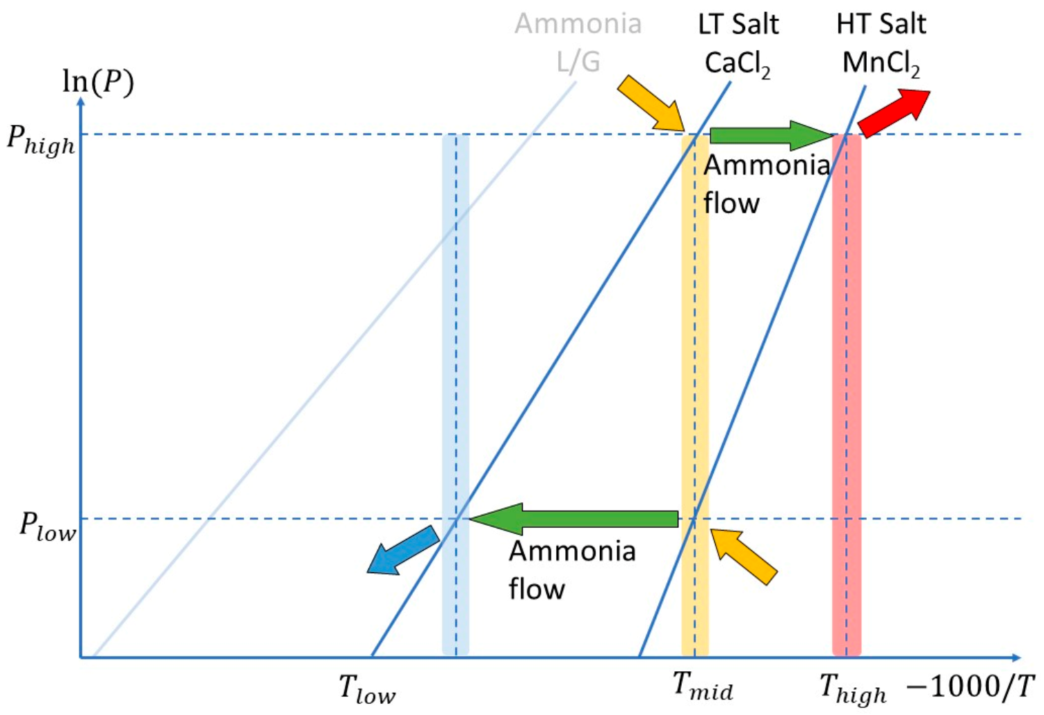
The resorption machine cycle has two main phases of operation and transitions between them. The resorption cycle is explained as followed and illustrated by Figure 1:
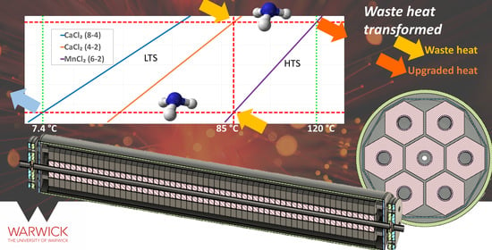
- The first phase is the high-pressure phase. Waste heat is delivered to the low temperature salt, the salt desorbs refrigerant, and the pressure rises in the system. Ammonia begins to adsorb in the high-temperature bed and the temperatures in both beds climb the Clapeyron lines until at the Phigh condition in Figure 2. At this point, high-temperature (useful) heat is recovered and returned to the industrial process. The transition between pressures takes place over a short period, and the heat is delivered over an extensive period.
- The second phase resets the system. Cooling water is delivered to the low-temperature bed initiating ammonia adsorption, and the system pressure begins to fall. The beds drop down the Clapeyron lines to the low-pressure condition. Whilst this occurs, the waste heat is fed to the high-temperature bed to provide endothermic heat. The process continues at low pressure until the exothermic adsorption reaction is complete in the low-temperature salt reactor.
Apart from for instrumentation and controls, little electric power is required in the process. The absence of evaporator and condenser within a resorption system creates the opportunity for cheap manufacture, whilst its operation requires a limited electrical power input.
There are 17 absorption thermal transformers that are operational, as detailed by Cudok et al.; these are mostly in Asia, saving several thousand tonnes of CO2 per year [7]. This highlights the efficacy of heat transformers. They detail the challenges that are especially important when considering a UK market (hydrogen or otherwise). These are: size of technology; high capital cost; and length of cycle times. This work aims to discuss how resorption transformer systems, as presented here, can address those challenges and be part of decarbonising heat.
1.2. Ammonia-Salt Reactions
Reversible reactions between ammonia and halide salts are monovariant equilibrium reactions; this means the operation of a resorption machine can be represented by a Clapeyron diagram such as in Figure 2. Many solid sorbents and adsorbates have been used for sorption applications such as activated carbon-ammonia, salt-methanol, and silica gel-water [8,9,10,11]. Critoph discussed the merits of the adsorbates and highlights the potential efficacy of ammonia and methanol as refrigerants, the challenge with methanol being its working limits. He also highlighted the limits of water as a refrigerant [12]. Water and methanol systems tend to operate at sub-atmospheric pressure due to their boiling temperatures. Consequently, mass transfer phenomena can considerably affect the rates of reaction. Such refrigerants are better suited to refrigeration and energy storage applications.
Ammonia is a better suited refrigerant for thermal transformer applications, and one of the first key papers highlighting its suitability for upgrading heat is by Goetz et al. [6]. The reason halide salts reacting with ammonia are promising for resorption (particularly for thermal transformers) is their high adsorbate uptake and relatively quick reaction rates [13]. Furthermore, resorption systems are able to make use of the extensive variety of salts that can be paired, creating flexibility and enabling tailoring to the applications or temperatures required [14]. Pairings that were suggested by Goetz et al. include calcium chloride (4-2)–barium chloride (8-0) and manganese chloride (6-2)–calcium chloride (8-4) due to the relative reaction temperatures [6]. Work by van der Pal and Critoph suggests that both calcium chloride reactions (8-4-2) can be considered due to the relatively close isosteres [13]. For future applications, it is worth noting that, in the case of pairs of different types of salt (e.g., sulphate and bromide), the equilibrium lines may cross on the Clapeyron diagram; this creates further applications with multiple temperature outputs [6].
1.2.1. Introduction to the Thermodynamic Characteristics and Reaction Kinetics
Key to the effective design of a generator is understanding the reaction kinetics and transport phenomena during a reaction cycle between ammonia and the halide salt (usually within a conductive matrix). A number of approaches were taken in the 1990s to develop a model for the reaction behaviour, which were then evaluated against various experiments. Contemporary experimental work tends to use either a gravimetric suspension balance test cell, or large-temperature-jump testing. This is then applied to a model, often based upon the methods presented in the 1990s. This paper will first consider the material and testing methods before an overview of the methods used to model and understand the reaction behaviour.
1.2.2. Testing Methods from Literature
Moundanga-Iniamy and Touzain studied sorption reactions between magnesium chloride and ammonia [15]; they tested pure magnesium chloride and magnesium chloride-natural graphite powder mix at a molar ratio of 1:5. They observed three equilibrium lines for differing moles of adsorbed ammonia (6–2, 2–1 and 1–0 moles) when testing with gravimetric methods. The production of the composite appears challenging, requiring six hours of heating a mixture of graphite powder and manganese chloride at 580 °C [15]. Touzain and Moundanga-Iniamy build on this work with their colleague Atifi, where they observe that the addition of graphite improves the heat and mass transfer, avoids agglomeration, and report improved reaction cycles of 30 min. Interestingly, they also record X-ray diffraction and neutron diffraction data of the composite and ammoniate and were able to deduce the shape of structure of the lattice when bonded to ammonia [16,17].
Mazet et al. conducted tests for a reaction chamber loaded with nearly 700 g of calcium chloride [18,19]. The simple experiment involved external heating and monitoring the temperature at a number of points across the radius. A notable observation was “…the quasi-simultaneous evolution of the two reactions”. Their conclusion is based on observing smooth temperature profiles. This is interesting, although different stationary temperatures can be seen in some of the more external radial readings during the evolution of the reaction. Additionally, the radial conversion plot has anomalous results, which need to be considered or the tests repeated. The main observations by Mazet et al. were that the size of their reactor bed enabled large temperature gradients to be observed during the process, and they conclude it is key to optimise the thickness of the salt bed [18].
More recently, there have been two main approaches to enable salt characterisation and testing: using gravimetric magnetic suspension balance equipment; and using the large temperature jump (LTJ) technique. A number of tests have been performed using a gravimetric suspension balance [20,21]; typically, this is operated by holding the test cell at a fixed temperature whilst changing the pressure using a liquid ammonia reservoir. The test process is therefore gradual, and the temperature of the material is not monitored [22,23]. This raises questions about its effectiveness for providing empirical data for sorption machine design. The LTJ method appears more effective, as it is designed to mimic the behaviour in sorption machines. Dawoud and Aristov pioneered the LTJ method to observe the evolution of sorption reactions [24], and it has been used many times to observe reaction dynamics [25,26,27].
Adapting this method to test ammonia-salt reactions has proven effective to observe phenomena that would be missed by gravimetric methods. For example, Atkinson et al. observed a peculiar behaviour at low pressures when ammonium chloride reacts with ammonia, with a spike in the temperature and a change in reaction behaviour [3]; furthermore, Hinmers and Critoph observed a superheating effect when barium chloride and ammonia react [2]. The LTJ method utilises large expansion volumes, which ensure the pressure change is low, similar to working sorption machines. The simple design also enables measurement of the material temperature improving understanding of the reaction behaviour.
Sharma et al. deploy a testing method, which essentially employs pressure jumps (rather than temperature jumps, performed by manually opening valves) to test ammonium chloride and potassium iodide [28]. The testing does not appear to be robust; they conclude that different isosteres occur at different concentrations of ammonia within the salt; this conclusion is uncertain due to the test method. They then choose to perform calculations neglecting this finding, which further brings this conclusion into question. Isobaric conditions are used to plot their differing isosteres, but the conditions where construction lines are applied clearly show a graduation in the pressure—so, the isobaric assumption is incorrect (N.B. the plot is a log scale exacerbating the error). This is important, particularly as this obtainment from a construction line is not shown for ammonium chloride, which shows conditions that are far from isobaric. The methodology is also confusing as the material is left to reach equilibrium, but equilibrium state-points are taken when the behaviour is transitory [28]. Values observed are when the equilibrium conditions are changing, and this is why hysteresis is observed. The irreversible effects of hysteresis should not be observed if allowed to equilibrate, since hysteresis and irreversible behaviour is a function of transients of transport phenomena. A better approach would be monitoring the final conditions after the pressure jump (when equilibrium conditions are reached), and not attempting to draw a straight line across dynamic temperature behaviour; this could produce an accurate unified line for the isosteres. Much of their work focuses on the idea that hysteresis always occurs, but an improved practical example that contradicts their work is shown by van der Pal and Critoph.
In the work by van der Pal and Critoph, they step a large reactor up and down the isostere by changing the temperature without hysteresis [13]. The stepping-up effect is to change the conditions and then leave to settle and then change again, thus observing the material under equilibrium conditions. Hinmers et al. also showed that a very slow reaction in a modified LTJ was able to produce cycles with reduced hysteresis for barium chloride and manganese chloride [29]; this led to them recording a single heat of reaction for both adsorption and desorption, rather than the erroneous recording of a different enthalpy of reaction for adsorption and desorption, which is also affected by the concentration of adsorbate [28]. Furthermore, Atkinson et al. observed no hysteresis when testing ammonium chloride in an LTJ, also recording a single heat of reaction [3].
It is clear that LTJ testing is the most effective way to observe the reactions, presenting a simple case that can be modelled and removing uncertainties found with other methods. Gravimetric testing has missed key data, and modelling based on it has often carried large factors of error. The conditions in an LTJ are similar to those in a working system, and a well-designed LTJ can be used to evaluate geometries and material sizes prior to testing at scale.
1.2.3. Modelling Reaction Kinetics
Key to analysing experimental results is constructing an effective model; in the literature, there are a number of approaches that have been taken. Some work has taken the approach to approximate a reaction rate equation, simply by fitting the reaction-rate/advancement to an exponential function. Other approaches have been highly theoretical with considerations of the transport phenomena. An et al. provide possibly the most comprehensive review of the mechanisms and kinetic models used to predict the behaviour of ammonia-halide salt reactions; they detail the methods taken by researchers over the last 30 years and examine their approaches so we can improve our own understanding [30].
An et al. conclude in their review paper that little attention has been paid to reaction kinetics in the years prior to its publication; rather, researchers have focussed on performance results [30]. A prime example of this is the work using an exponential function with a time constant. This was capable of approximating reaction performance [25,31,32], but this black-box-type approach lacks flexibility and is prone to error when scaling up. A theoretical approach was taken by Lebrun and Spinner; this was perhaps one of the first methods used to dimension a working system from dynamic reaction results [33,34,35]. Lebrun and Spinner present reaction kinetics in an analogical form, assuming that the limiting factor is the chemical reaction rate. They base this conclusion on two reactions between methylamine and calcium chloride and derive the following equations [35].
The general form of the equation:
For adsorption
- –
- Reaction (I)
- –
- Reaction (II)
For desorption
- –
- Reaction (I)
- –
- Reaction (II)
The functions can be seen to have pseudo-reaction energies that incorporate the gas constant and contain a pseudo pre-exponential factor; they also include pseudo-orders of reaction that do not correlate to a real order of reaction. They evaluate two consecutive/simultaneous reactions; hence, (I) and (II). The method is very interesting and has inspired much subsequent work including this paper, but the number of constants makes the process unnecessarily complex; too much weight is put on the pseudo-orders of reaction, when they infer that all but one are equal to 1. The kinetic coefficients can be seen to change depending on the packing density and the proportion of binder. The fact that these values have an optimum—and this is presented as a way to optimise the composite performance—suggests perhaps this value is responding to improved conductivity and thus reaction rate, and not actually predicting the kinetics. This suggestion is due to the fact that observations in more contemporary work show heat transfer is a key parameter for performance [2]. The flaw in this method appears to be they: “…consider only the global exchanges between the reacting medium and the heat transfer fluid.” [33]. For such a complex approach to the reaction rate equations, it would have been more instructive and a more accurate test if the model was local. Nonetheless, this work is a key step in design based on dynamic reaction results [33].
Another approach was taken by Mazet et al., again observing the reaction between methylamine and calcium chloride [18,19]. Their approach was to decouple the kinetic and thermal equations and resolve the kinetic equation for , independently of heat transfer. This can then be used in part to derive the local heat transfer effects. They again present two kinetic equations for two reactions, with the potential for simultaneous reactions occurring.
Mazet et al. describe from Equation (9) as a term to weight the expression for reversible heterogeneous reactions by the difference between operating conditions and equilibrium conditions [18]. Therefore, the final kinetic equation is in a similar form to that for surface kinetics for catalytic reactions, as shown in Equation (11) [36]; in Equation (7)—the rate of conversion—is a function of the conversion , to the power of a pseudo-order , multiplied by a rate of reaction term that encompasses kinetic term and the displacement from equilibrium (derived from Equation (11)).
The choice of a displacement from equilibrium term is important when we consider that the preponderant effect on the adsorption reaction is the driving force created by the extent of the negative deviation—or the lower the temperature relative to the equilibrium conditions. During adsorption, in Equation (9), the Arrhenius term would decrease, but an increased reaction rate is observed even as the negative temperature displacement increases (highlighting the dominance of the displacement from equilibrium). Additionally, the preponderance of the deviation from equilibrium can also be seen in the desorption reaction. The choice of to express the deviation from equilibrium conditions rather than temperature ensures the separation of the kinetic and thermal expressions in their model, but still reflects the driving force.
The function describes global advancement and is shown to predict with success. They explain the Arrhenius term has a limited effect, as the rate is dominated by the deviation from equilibrium; furthermore, it is “practically equivalent to a constant”, and it is therefore not possible to extract the parameters and E, from Equation (9). Inadvertently, the global model appears to be replaced with a local (one-dimensional) model, where , , and are a function of the radius [18].
Lu et al. developed a phenomenological model that helps to further our understanding of some of the transport phenomena involved [37,38]. The model evaluates a case where the rate limitation is both heat and mass transfer. The model is presented for a halide salt reacting with ammonia and considers the reactions at grain and pellet level in the form of a shrinking core reaction model. They compare a “simplified” and “general” model for their effectiveness [38]. Their tests on pure salt show cycles that occur over hours. The method is novel and shows some insight into the performance when mass transfer limitations need to be considered [37]. Cycles of this duration are restricted to energy storage processes, and much work has been done showing that ammonia-salt reactions in some form of graphite composite overcome issues with mass transfer and cycle quickly.
More recent work has looked at analogical models to predict the kinetics; An et al. evaluate the effectiveness of an exponential, power function, and a linear model. They conclude that only the linear model is (relatively) reliable in predicting the kinetics [21,22]. The form of this model is similar to that presented by Mazet, discussed earlier in this section. Adsorption is shown in Equation (12) and desorption in Equation (13).
They use the equations to predict the behaviour of a manganese chloride and expanded natural graphite composite, reacting with ammonia. A plot is presented, showing results between ±20% deviation [22]. Furthermore, even within these large bounds, they show that the constants vary between the different tests, i.e., they are not true constants. The challenge when interpreting is that one cannot see the cycle results from the model; if the enthalpy of reaction is calculated from results from the Rubotherm magnetic balance, this could be the source of some of the error.
Hinmers and Critoph developed the Mazet model and were able to effectively predict the behaviour of barium chloride in expanded natural graphite sheet reacting with ammonia. They observed that the rate of heat transfer into the composite was the rate limiting factor [2]. This model was then developed, taking a new mass-based approach wherein they derived new equations to describe the salt/adsorbate composition relative to the conversion of the reaction; this method presents an empirical way to show the consecutive reactions that can occur in salts such as calcium chloride [29]. Their results show an effective method to predict the performance of manganese chloride and barium chloride results, over diverse testing at different scales and with unified constants.
Applying the model by Hinmers et al. presents a method to simulate the multi-reaction behaviour of calcium chloride and appears to be the most effective approach.
2. Materials and Methods
The salts considered in this paper were first proposed by Goetz et al. [6]. The pairing of chloride salts ensures the near-parallel nature of the Clapeyron lines; this is important as the lines are presented as a function of the enthalpy, and optimal performance will come from parallel lines. Identifying which pairs perform best is important in designing a test cell.
The salt adsorbent is hosted in an Expanded Natural Graphite (ENG) matrix (SIGRATHERM® Graphite Lightweight Board, ECOPHIT® L10/1500). This overcomes agglomeration and increases the conductivity. The even distribution of the salt crystals throughout the ENG also ensure that the reaction rate is limited by the rate of heat transfer into the composite [29]. The material is prepared by submerging cut ENG in a saturated solution; this is then placed in a vacuum for 24 h, and the ENG is then dried. Atkinson et al. detail the preparation method [3].
2.1. Clausius-Clapeyron Lines for Envelope of Operation
The operating temperatures and pressures for a resorption system are derived from the isosteres for the selected salt pairs. The variables are the salt pairs and the middle heat temperature. The middle heat (which, in this application, is the waste heat), enables an upgraded heat temperature to be derived from the pressure at which the equilibrium changes for the low-temperature salt (LTS) at ; and the heat sink temperature is derived from the pressure that the equilibrium changes for the high-temperature salt (HTS) at . These form the high and low pressures and temperatures, respectively. This is represented in the ideal cycle shown in Figure 2, where the horizontal lines are the pressures, and the vertical lines are , , and from left to right.
The most evident application for a transformer is the recovery of heat from steam condensate and transforming it to produce further steam; therefore, the waste heat is expected to be provided below 100 °C and is used to raise steam above 100 °C. To ensure heat transfer and a driving force for reactions, heat should be provided 10 °C hotter and emitted to 10 °C lower than the reaction temperatures. Therefore, as a rule of thumb, , the middle temperature at which the waste heat is provided, is taken at ≤85 °C, and must be high enough to raise steam. For a transformer to be applicable in the UK, it needs to be able to expel heat at to cooling water, so for proof of concept, 25 °C is suitable; operating temperatures will be revisited in the discussion section.
Optimal performance in a resorption system will come from paired salts with near parallel reaction isosteres; (di)chloride salts’ isosteres are quasi parallel in nature. If we consider the collation of chloride salt equilibrium lines by Neveu and Castaings for the temperature requirements detailed, we can see that of these salts, barium chloride, calcium chloride, and manganese chloride appear suitable [14]. Goetz et al. also suggest these salts for a variant of the transformer process [6]. The most likely pairing is CaCl2 and MnCl2; the operating pressures and temperatures are in a suitable region, the stoichiometry is proportional, and manganese chloride has already been proven to produce fast cycle rates, whilst van der Pal and Critoph have shown the applicability of calcium chloride [13,29].
2.2. Large Temperature Jump and Experimental Results
An LTJ method previously described has enabled the gathering of reaction data for barium chloride, manganese chloride, and ammonium chloride [3,29]. A diagram of the LTJ experimental set up can be seen in Appendix A.
A resorption machine is likely to use calcium chloride as one of the salts, as previously detailed. Using this approach, it is possible to obtain data for the onset of reaction, and a unified heat of reaction for adsorption and desorption for either calcium chloride reaction with ammonia, creating a basis for modelling.
The calcium chloride and ENG composite is held in a heat exchanger, which is connected to a large expansion volume. The expansion volume reduces the pressure rise, but the pressure rise is substantial enough to observe the evolution of the reaction. The heat exchanger is fed by oil or water from two Huber thermostatically controlled baths, and switching between them causes the temperature jump effect. The temperature of the wall in contact with the material and the centre or outer temperature of the material are measured. An accurate wall temperature is taken using a pair of grounded thermocouples, in which a wire from each is used to measure the induced voltage so that the junction becomes the wall of the heat exchanger itself. LTJ tests have been run in a tube arrangement with the composite within the tube and heat exchanger fluid in the shell, and in a shell arrangement with the composite in the shell and the fluid in the tube [29]. A unified heat of reaction was observed by modifying the experiment to remove the expansion volume, performing an isosteric temperature change (ITC). This was named as such because the method attempts to track the isostere closely by setting a bath to slowly ramp up and down for cycles in excess of 8 h. In an ITC test, the pressure versus temperature plots had reduced hysteresis, and the gradients of the adsorption and desorption Clapeyron lines were very similar (quasi-parallel). An average therefore presents a good estimate for the heat of reaction derived from the Clapeyron relationship.
2.3. Modelling Calcium Chloride Results and Obtaining Parameters for Reaction Kinetics
The calcium chloride reactions from the LTJ can be modelled individually and as a pair so that simulations can be undertaken to optimise performance. This is performed using the model presented by Hinmers et al. [29]. To do this, the results of the individual reactions are fitted first to identify the parameters. These are then compared with tests at different pressures and further evaluated in tests that cross two phase changes.
The modelling objective is to identify the constants and for desorption and adsorption for both reactions. The kinetic equations for desorption of two reactions from state to and from to are presented for desorption for both reactions in Equations (14) and (15). Calcium chloride in state is CaCl2∙8NH3, is CaCl2∙4NH3, and is CaCl2∙2NH3.
3. Analysis and Results
With the information obtained from LTJ testing, it is possible to begin optimising a reactor design. Key performance metrics are the predicted COP and the peak specific mean power (SMP).
3.1. Salt Categorisation and Calcium Chloride Test Results
Calcium chloride LTJ results with a substantial temperature jump () show both individual phase changes for reaction 1 and 2 in one cycle, as shown in Figure 3. These can be seen as the isothermal conditions that coincide with a rise in pressure. In fact, the differing rates of the two reactions can be seen by the change in the rate of the pressure change. In some cases, at lower pressures, an apparent single-phase change occurred across both reactions.
The Clapeyron lines for prediction of the onset of desorption and adsorption are plotted next to Clapeyron lines observed by the ITC testing method (for the heat of reaction ) for calcium chloride-ammonia (8–4) reaction in Appendix B. The resultant values for and are shown in Table 1. and are not values for a heat of reaction; they are derived from the Clapeyron equation and just predict the onset of reaction, and only provides a value heat of reaction. These data provide the basis for predicting the onset of reactions and a single value for adsorption and desorption.
The experimental results show superheating and subcooling effects pre-empting the phase changes that have previously been observed for barium and manganese chloride [29]. A single adsorption reaction (that spans both phase changes) can be seen in Figure 4; the first cycle shows two phase changes, but during the second cycle, only one is observed. At all pressures, it was possible to study each phase change independently by controlling the temperatures to include only one reaction. In Appendix C, the recorded points at which the onset of reaction occurs are plotted to show how the isosteres were derived. When one adsorption reaction appears to occur rather than two, another line has been plotted from the onset conditions, and it appears midway between the two isosteres. The observations generally show an evolution through both reactions one after the other; but on a granular level, different sized grains could be reacting/finishing at different rates. The subcooling effect may present the conditions for the subsequent reaction to also initiate at the same time.
3.2. Model Results and Identified Constants for Reaction Kinetics
Using Equations (14) and (15), it is possible to simulate the reaction data for calcium chloride. The modelled results of calcium chloride LTJ tests can be seen in Figure 5. The kinetic parameters were identified using trial and error following some logical steps. The first step is to derive an active fraction; the salt is assumed to have an active fraction of salt that is accessible to the ammonia and capable of reacting, which is the percentage of the stoichiometric mass reacting that is observable over the cycle time. The argument for this is that it can be observed that there is a clear starting and finishing point (i.e., stationary pressure before and after) when LTJ testing. The active fraction can be identified by matching the pressure rise in the results to a fraction of the reacting mass; the remaining mass (inactive) is accounted for in the model as a thermal mass.
Following this, it is necessary to evaluate the heat transfer resistance. This is calculated as a ‘gap’ of ammonia gas and derived from the conductivity of ammonia over the nominal length of gap to provide a heat transfer coefficient value. This is validated with a temperature jump with no sorption reaction. From this point, and can be identified. These terms have a limited effect on the rate of reactions in this composite, as it is primarily influenced by the rate of heat transfer into the material. However, adjusting the constants produces a better fit of the temperature curve and the pressure curve. The resultant fittings for individual phase changes can be seen in Appendix D, Appendix E, Appendix F and Appendix G. The derived constants were then used to simulate the double reactions, as shown in Figure 5. The derived values for the reaction rate constants from Equations (14) and (15) can be seen in Table 2. The active fraction observed for calcium chloride is 0.8. This aligns with previous findings for the active fraction for manganese chloride and barium chloride [29]; it is also equivalent to the value used when modelling by Lépinasse et al., providing confidence in the value [39].
In Appendix H, the simulated results are presented for the double adsorption reaction with an apparent single phase change. The model performs two reactions; this makes sense when the nature of the lumped parameter model is considered. The actual result may have crystals reacting at different temperatures and the thermocouple reads a regional temperature averaging local effects.
3.3. COP Calculation
The COP can be calculated to assess the thermal efficiency for different sizes of material and tube combinations. To assess this, a unit cell is defined to represent the reactor geometry. The assumption is that the reactor is composed of uniform cells in a bundle arrangement, with an equal ratio of materials per length throughout the bundle. A unit cell is defined in Figure 6. This comprises salt-ENG composite, a stainless-steel tube, and heat transfer fluid per unit length. This mass ratio can be used to observe different pairs when we factor in stoichiometric ratios and uptake of salt into the ENG. This can be used to assess both shell and tube side positions of the composite, but external placement is most likely because inert thermal mass ratio is less.
The heats of reaction calculated from the ITC tests were used for the COP calculation, and equilibrium data for the onset of reaction provided the temperature values. Predicting the COP requires evaluating the heat in and useful heat out, accounting for the thermal masses per mass of salt in the low temperature bed, as shown in Equation (16). The heat in is assumed to be: the sensible heat to heat up the low-temperature salt ; the sensible heat to heat up the mass of ammonia gas desorbed during the high-pressure phase, ; the reaction heat of desorption in the low-temperature bed during the high-pressure phase, ; and the reaction heat of desorption in the high-temperature bed during the low pressure phase, . The useful heat produced is the heat of adsorption recovered from the high-temperature bed during the high-pressure phase of the process, , minus the sensible heat required to heat the high-temperature bed, ; this has to come from the adsorption heat due to the temperatures required. The calculation is conservative, and furthermore, some of the sensible heat in both beds could be recovered by employing heat recovery—this will be visited in the discussion section.
Drawing the Clapeyron diagram for the salt pair helps to clarify how this is calculated. The sensible heating () occurs during the phases where the temperature is changing up and down the isosteres. The key temperature points are identified by the markers seen in Figure 7. In the case of the barium chloride and calcium chloride pairing, the isosteres cross; this is impossible, as the true position of the lines would differ at these conditions. However, the calculations use a unified heat of reaction, which has a much greater value than sensible heating, and so the error relating to the sensible heating will be small. The calculation is just to determine the effectiveness of pairings and sizing. In Figure 7, three combinations are presented. The first two pairs are suggested by Goetz et al. [6], and the final option is for calcium chloride utilising both reactions as they occur closely. Both reactions of calcium chloride cannot be used when it is a high-temperature salt, as recoverable heat would be produced at two temperatures.
The option to use both calcium chloride reactions is preferential; van der Pal and Critoph tested both reactions in a single reactor as part of an adsorption heat pump, and no adverse effects were observed. The use of both reactions enables an increase in the power density of the calcium chloride bed. Corresponding values calculated for the estimated COP for both resorption pairs can be seen in Table 3; this estimate is performed based on a unit cell in Figure 6. This presents an idea of the performance; real COP performance will be lower due to effects of the shell and other thermal masses.
3.4. Specific Mean Power and Peak Delivery
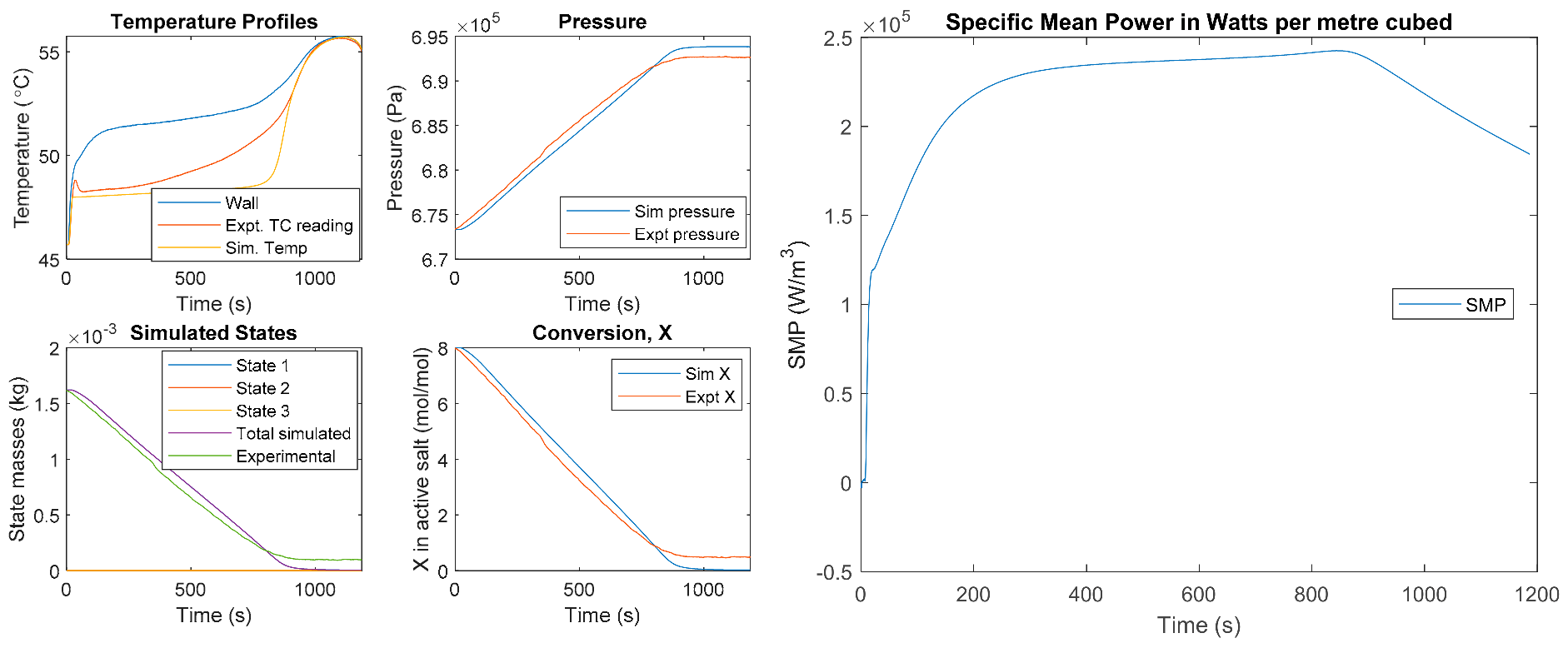
Using the reaction model that applies Equations (14) and (15) and the identified terms [29], it is possible to assess the specific mean power. The model can then be used to predict the power density based on assessing the cumulative heat flow in or out of the boundary node during the cycle. The SMP (W/m3) can be observed over the evolution of the reaction, and the peak value can be used to predict the power density of a machine. The SMP is calculated from the sum of cumulative heat into (or from) the salt-ENG composite and the cumulative heat to the steel and heat transfer fluid, divided by the time and the total volume of the cell (the cell represented in Figure 6). An example of a shell-side test for experimental data of barium chloride is shown in Figure 8, with the resultant SMP plotted.
It was also possible to infer potential power density performances for different tube sizes. This could be performed by creating a ramp in wall temperature in simulation and assessing the different peak SMP values that result for different tube sizes. The calculations do not account for realistic heat transfer from the wall to the tube but give an idea of how different sized tubes can perform. The working machine requires a 10 °C driving temperature to ensure heat transfer. Initially, the program was set to ramp the wall temperature 10 °C and the SMP was observed over a range of standard tube sizes (½” ¾” 1” outer diameter tube) and a range of different sizes of samples (some can be seen in Appendix J). This was then validated with a test in the shell-side large temperature jump to ensure peak SMP performance was acceptable.
The peak SMP in Figure 8 is not high enough to be attractive. During the temperature jump, the bath quickly recovers to its set temperature, but the measured wall temperature is lower than the temperature of the bath, as the laminar flow of the oil reduces the amount of heat delivered to the reactor. The wall temperature is effectively being suppressed, showing there is extensive heat transfer resistance from the fluid to the wall. The reaction is heat-transfer limited, so improving the heat transfer is key to achieving a higher power density, as a faster rate of reaction will increase the power. Another option to increase the rate of heat transfer is to increase the size of the tube. Different sizes of tube were simulated with an artificial ramp in wall temperature, and some results can be seen in Appendix J. This gives an idea of the relative performances of different tube sizes, but the results show a higher SMP than what would be obtainable in practice due to the (unrestricted) rapid rise in the simulated wall temperature. The results from tube size analysis are discussed further in the discussion section, exploring the effect of this on the COP. Improving the peak SMP by increasing heat transfer is important, as a larger size of composite relative to tube can be employed, which would increase the COP of a system. Therefore, improving heat transfer is a primary focus.
To improve the heat transfer from the fluid to the tube, the heat transfer fluid was changed from oil to water, and CALGAVIN hiTRAN® Thermal Systems tube inserts were implemented in the tube to increase turbulence. To improve the heat transfer from the tube to the composite, hole saws were manufactured, and smaller inner diameters were cut and pushed onto the tube, with measures taken to discourage cracking. The efforts to improve heat transfer can be seen in Figure 9.
ENG samples cut to 11.9 mm and dosed with salt were the smallest size of inner diameter that it was possible to push over the 12.7 mm tube [29]. The effect of improving the contact (and the addition of fluid tube inserts) enabled a final sample—32 mm hexagon, 16 mm apothem—to produce a SMP of around 1.4 kW/L, as shown in Figure 10. A hexagon shape was used and modelled as a circle of the same area, with a 33.6 mm diameter. A hexagon shape was decided on to form a tube bundle arrangement in a heat exchanger.
4. Discussion
The LTJ and ITC testing has been successful; the identified parameters enable accurate simulation of salts with potential for a resorption transformer. By identifying a value for the heat of reaction, it is possible to estimate the COP of a working machine and the SMP. Efforts to improve the heat transfer have also proven successful.
4.1. Optimisation
When analysing the COP and the peak SMP, there is a trade-off between the two. When considering the COP, the thermal masses become very important. The ratio of active material (composite) to stainless steel and water directly affects the COP, and by increasing the former, a higher COP is obtained. The SMP is a function of the material volume and the rate it reacts. On the outside of a tube when varying the radius, the results suggest the thinner the composite the faster it cycles, and the higher the peak specific mean power; this tends towards a larger tube with a thinner composite layer due to the increase in heat transfer area. An initial conclusion could be that increasing the tube size is beneficial as a higher heat transfer area would increase the heat transfer (assuming the same heat flux). Alas, increasing the tube size increases the thermal mass of the fluid and steel, and so a higher SMP is marred by a drop in COP. Results reviewing the COP for different tube sizes can be seen in Appendix K, showing that the larger tubes suffer reduced COP values. From evaluating the effects of tube size and material size on COP and SMP, a final size was settled upon for a 16 mm apothem hexagon over a ½” tube. This was then used to consider the different salt pairs’ COP performance in Table 3.
The final value for the power density is more than 1 kW/L for one bed; improving the heat transfer from the fluid to tube and reducing the contact resistance were therefore successful. It is worth noting that the SMP will effectively be halved when paired with another reactor. Future work should look to improve the heat transfer further to increase the SMP. The improvement of heat transfer to the composite gave rise to a smooth SMP, suggesting constant heat flux, which is beneficial for system design due to continuous heat delivery.
The 33.6 mm circle (hexagon with a 16 mm apothem) was used to calculate the COP values in Table 3. The COP estimate is a reasonable result, but the calculation does not account for the added thermal masses of the shell and end plates of a reactor, so although conservative in terms of the sensible heating of the tubes and material, it is an over-estimate. In practice, some of the sensible heat may be recovered by pairing two pairs of beds and applying heat recovery.
When looking at the Clapeyron relationship plots for the paired salts, the effect of the hysteresis can be observed. The hysteresis does lower the COP, but marginally through increasing sensible heating. The main challenge of the hysteresis is it reduces the temperature lift, and the sink temperature also drops lower. This could cause the system to be ineffective, and cooling water could not provide the heat sink required. Results from van der Pal and Critoph, however, showed their reactor had reduced hysteresis in operation [13]; whether this can be replicated in resorption will be key to conception of resorption transformers in industry.
The SMP improvements were performed with barium chloride, using water and inserts in the tube. Only barium chloride was analysed as the reaction temperatures for manganese chloride and calcium chloride are typically too high to be used with water as the heat transfer fluid (within this experimental set up). All salts were tested for contact, however, and the samples did not break throughout. Using empirical data for salt uptake and stoichiometric molar ratios for the reaction, it is possible to estimate the lengths of paired reactors—this provides a relative understanding of potential power densities. Based on the peak SMP of 1.4 kW/L, a 3 kW reactor would require a volume of 4.29 L of barium chloride composite and tube—the SMP value is halved to account for driving the second bed. Based on the moles of desorbed ammonia from this mass, masses of other salts can be calculated, and empirical data for the mass of salt/composite enables a length to be calculated. The results can be seen in Table 4, calculated from the MATLAB file attached in the Data Availability Statement.
These results present relative reactor lengths shown in Appendix K. This illustrates that the pairing of barium chloride (8-0) and calcium chloride (4-2)—which had an apparent high potential COP—is not viable, as the power density is very low. The best pairing is calcium chloride (8-4-2) and manganese chloride (6-2).
4.2. Design Remarks
Based on the lengths presented, it is possible to form a reactor design. The calcium chloride (8-4-2) data from Table 4 is taken as a basis, and the rest of the design is considered as follows. The low pressures that are noted in the calcium chloride and manganese chloride pair, which can be seen in the Clapeyron diagram in Figure 8, suggest that the mass velocity at low pressure could cause damage to the ENG matrix. To address this, a design is proposed with gas channels to enable flow. The samples also swell on adsorption, so this must be considered. To minimise sensible heating to the shell, a folded aluminium plate is proposed: not only does this create a stagnant layer of gas against the shell to reduce heat loss, it forms triangular channels for the gas flow. This is held in place by a spot fitted ring of aluminium at each end. The proposed design can be seen in Figure 11. A gap of 2 mm is sized between the composites; this ensures space for swelling and a gas channel.
The ends of the reactor also incorporate a void to provide gas passage. The extra void volume in the reactor is a relatively small increase, as the ENG has a high void volume. The sizing also incorporates some space for the swelling of samples. A comprehensive design is presented, showing a cutaway of a reactor, incorporating end voids for flow sized internally to a ½” pipe; the addition of one at each end can half the flow rates. The ends shown here also incorporate a manifold to distribute the flow between the seven tubes with the same flow rate, using an orifice and machined channels.
The MATLAB file attached in the Data Availability Statement calculates the reactor size for two salt reactors based on the choice of pairs and depending on the power specified; the file assumes equivalent geometry for both and scales based on length required for a seven tube bundle. The model then calculates the COP based on a unit cell—which forms the data in Table 3. Within the program, there is a calculation for the full shell and other components specified in Figure 12, including masses and a calculation of thermal masses . Thermal masses are typically under-reported, as alluded to in the literature review section and described by Gluesenkamp et al. [40]. The thermal mass output can be used to consider how the shell could affect the COP. Simple calculations can be taken using it, such as one described in the attached txt file, but accurate COP estimates are not possible without a reaction model for two beds incorporating the heat transfer.
4.3. Challenges and Next Steps
The primary challenge to the successful use of the composite was the rate of heat transfer. The contact with the material and the tube was improved using tighter fitting samples over the tube, as explained in Section 3.4. Prior to improving the heat transfer, initial testing used silicone oil, as this offers a wide range of testing temperatures. Some later tests with barium chloride used water as the thermal fluid, but temperatures are restricted, so it was not possible to test manganese chloride or calcium chloride. The final resorption generators will be used with high-pressure water; this will enable operating temperatures suitable for the reactions of the salts. Furthermore, steam condensate is the most practical feed fluid for a resorption system and is a high-pressure water feed, so emulating this in experiments is useful. The generator design proposed here will be installed in a resorption test bed and will be evaluated using the ThermExS rig (built by Spirax Sarco) at the University of Warwick. This can supply hot water at up to 250 °C and glycol down to −50 °C. The heat transfer is key to the performance of the system and may require further enhancement. The COP results are promising, but they are relatively low. This means real systems will need to employ a greater (radial) size of sample and need to cycle faster. Therefore, it is imperative to reduce the heat transfer resistance. This will be key to the realisation of resorption systems attractive to market. At this stage, it is apparent that working systems will require two beds out of phase to be employed. This enables heat recovery between beds out of phase (the HTS bed that needs cooling will heat the HTS bed that needs heating as both systems transition). This would raise the COP to reasonable levels by improving heat utilisation.
5. Conclusions
LTJ testing has identified the reaction kinetics and equilibrium data for calcium chloride reacting with ammonia, as per the two reactions: CaCl2∙8NH3 ⇌ CaCl2∙4NH3; and CaCl2∙4NH3 ⇌ CaCl2∙2NH3. An accurate heat of reaction was also estimated for both reactions. Using these data, it was possible to formulate simulations to discuss the design of a reactor for a transformer. The results show that, from the salts discussed, the only viable pair is calcium chloride (8-4-2) and manganese chloride (6-2). A proposed initial reactor design for calcium chloride has been presented with anticipated sizing. The design presented is for the measured SMP or power density of 1.4 kW/L observed with barium chloride in the LTJ. Future testing of the design will be successful if the reactors produce the expected power delivery of 3 kW and a COP in the range of 0.3. The dynamically measured COP can then be assessed with modelling to calculate how heat recovery could further enhance this value. The experimental results show that improving heat transfer is the best way to further enhance the prospect of resorption systems, and this will be necessary to achieve a marketable heat transformer.
Author Contributions
Conceptualization, S.H., G.H.A., R.E.C. and M.v.d.P.; methodology, S.H., G.H.A., R.E.C. and M.v.d.P.; validation, S.H.; formal analysis, S.H., G.H.A. and R.E.C.; investigation, S.H. and G.H.A.; resources, S.H., G.H.A. and R.E.C.; data curation, S.H.; writing—original draft preparation, S.H.; writing—review and editing, S.H., G.H.A., R.E.C. and M.v.d.P.; visualization, S.H.; supervision, R.E.C. and M.v.d.P.; project administration, S.H.; funding acquisition, R.E.C. All authors have read and agreed to the published version of the manuscript.
Funding
This work has been supported by two EPSRC projects: EP/V011316/1, “Sorption Heat Pump Systems” in support of Mission Innovation Challenge 7: Affordable Heating and Cooling, and EP/R045496/1, Low Temperature Heat Recovery and Distribution Network Technologies (LoT-NET). Further capital investment support was provided by the Energy Research Accelerator funded by InnovateUK.
Institutional Review Board Statement
Not applicable.
Informed Consent Statement
Not applicable.
Data Availability Statement
Supporting MATLAB® files are attached in the open access Warwick Research Archive Portal (WRAP) and are accessible through the following link: http://wrap.warwick.ac.uk/162466/ (accessed on 5 March 2022). The files with an attached text file present the MATLAB® file for the COP calculation and calculate the thermal masses of any reactors designed based on specified power and the geometries presented in this paper. The text file breaks down the sections of the MATLAB® file and presents how it could also be altered.
Acknowledgments
The authors would like to acknowledge their gratitude to Charles Joyce, technician for the Sustainable Thermal Energy Technology group, for technical support and extensive widget manufacturing.
Conflicts of Interest
The authors declare no conflict of interest.
Nomenclature and Abbreviations
| Arrhenius factor (varies) | |
| COP | coefficient of performance |
| concentration of component A (mol m−3) | |
| kinetic coefficient (s−1) | |
| 𝐸,𝐸′ | pseudo-activation energy (K−1) |
| ENG | expanded natural graphite |
| HT, HTS | high temperature, high-temperature salt |
| ∆𝐻 | enthalpy term (J/kmol) |
| ITC | isosteric temperature change |
| 𝑘, 𝑘0 | kinetic coefficient (s−1) |
| LT, LTS | low temperature, low-temperature salt |
| LTJ | large temperature jump |
| 𝑛, 𝑛′ | pseudo-order of reaction, and second reaction |
| 𝑚, 𝑚′ | pseudo-order of reaction, and second reaction |
| 𝑚𝑆𝐴𝐿𝑇 | mass of salt (kg) |
| 𝑃, 𝑝 | pressure (Pa) |
| 𝑄 | heat (J) |
| 𝑅 | gas constant (J K−1 mol−1) |
| ∆𝑆 | entropy term (J kmol−1 K−1) |
| SMP | specific mean power (W m−3) |
| 𝑇 | temperature (K) |
| 𝑡 | time (s) |
| 𝑋 | conversion |
| 𝑌 | conversion of 2nd reaction |
Subscripts
| salt in form A | |
| 𝐴𝐵 | change from form A to B |
| 𝑎𝑑𝑠., 𝑎𝑑𝑠𝑜𝑟𝑝𝑡𝑖𝑜𝑛 | adsorption reaction term |
| 𝐵 | salt in form B |
| 𝐵𝐶 | change from form B to C |
| 𝐶 | salt in form C |
| 𝑑 | desorption |
| 𝑑𝑒𝑠., 𝑑𝑒𝑠𝑜𝑟𝑝𝑡𝑖𝑜𝑛 | desorption reaction term |
| 𝑒 | equilibrium conditions |
| ℎ, high | higher conditions (temperature or pressure) |
| ℎ𝑒𝑎𝑡 | reaction heat term |
| ℎ𝑒𝑎𝑡𝑖𝑛𝑔 | sensible heating term |
| 𝑙, low | lower conditions (temperature or pressure) |
| 𝑚 | middle conditions (temperature), waste heat temperature |
| 𝑅𝐸𝐴𝐶𝑇 | reaction term (heat of reaction) |
| 𝑠 | adsorption |
Appendix A
Figure A1.
Initial LTJ reactor process flow diagram. Reprinted from Ref. [2].
Figure A1.
Initial LTJ reactor process flow diagram. Reprinted from Ref. [2].

Figure A2.
Shell side reactor process flow diagram. Reprinted from Ref. [29].
Figure A2.
Shell side reactor process flow diagram. Reprinted from Ref. [29].

Appendix B
Isosteres plotted from LTJ results. These are compared to those from literature presented by Neveu and Castaings [14].
Figure A3.
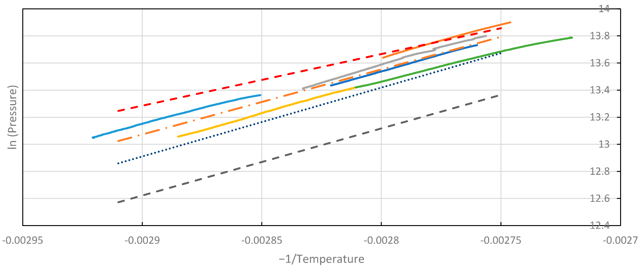
ITC Isostere plots for the calcium chloride 8−4 mol reaction with ammonia Exp. Are for the experimental lines plotted from the onset of reaction in the LTJ after any peak or superheat behaviour. Whereas the low hysteresis lines were performed by the slow reactions with the reduced volume and hour long cycle times. Note the reduced hysteresis.
Figure A3.
ITC Isostere plots for the calcium chloride 8−4 mol reaction with ammonia Exp. Are for the experimental lines plotted from the onset of reaction in the LTJ after any peak or superheat behaviour. Whereas the low hysteresis lines were performed by the slow reactions with the reduced volume and hour long cycle times. Note the reduced hysteresis.

Figure A4.
Plots for the 4−2 ammoniation reaction of calcium chloride: solid lines are for ITC isostere plots; dashed lines are the onset of adsorption and desorption (top and bottom, respectively); the dotted line is for the equilibrium line cited by Neveu and Castaings); the dot and dashed orange line is an isostere from plotting the average intercepts and gradients of the solid line ITC isosteres to illustrate the final result. It was difficult to obtain the values for this reaction, hence the number of plots, linear sections of the looping cycles were taken over a number of tests, and the average was calculated to estimate an enthalpy of reaction.

Appendix C
Equilibrium data points collected for calcium chloride adsorption at the onset of reaction (after any superheating/subcooling effect). The data is labelled based on the change in the number of adsorbed moles. During adsorption, seemingly, a single-phase change occurred; these were plotted, and the trend line can be seen in the middle of the two reactions.
Figure A5.
Equilibrium lines for calcium chloride adsorption, including the data for the apparent single phase change across 2–8 moles.
Figure A5.
Equilibrium lines for calcium chloride adsorption, including the data for the apparent single phase change across 2–8 moles.

Appendix D
Further examples of desorption simulation results from LTJ tests at 7 and 4 bar for (8–4) CaCl2 reaction.
Figure A6.
Desorption simulation results from LTJ tests at 7 and 4 bar for (8–4) CaCl2 reaction.

Appendix E
Further desorption simulation results from LTJ tests at 6 and 4 bar for (4–2) CaCl2 reaction.
Figure A7.
Desorption simulation results from LTJ tests at 6 and 4 bar for (4−2) CaCl2 reaction.

Appendix F
Further adsorption simulation results from LTJ tests at 7 and 4 bar for (4–8) CaCl2 reaction.
Figure A8.
Adsorption simulation results from LTJ tests at 7 and 4 bar for (4–8) CaCl2 reaction.

Appendix G
Further adsorption simulation results from LTJ tests at 6 and 8 bar for (2-4) CaCl2 reaction.
Figure A9.
Adsorption simulation results from LTJ tests at 6 and 8 bar for (2-4) CaCl2 reaction.

Appendix H
Simulation of adsorption reactions where the LTJ appears to show only one phase change.
Figure A10.
Simulation of adsorption reactions where the LTJ appears to show only one phase change.

Appendix I
Ramping simulations that provide basic evidence for deciding on sample dimensions before
Figure A11.
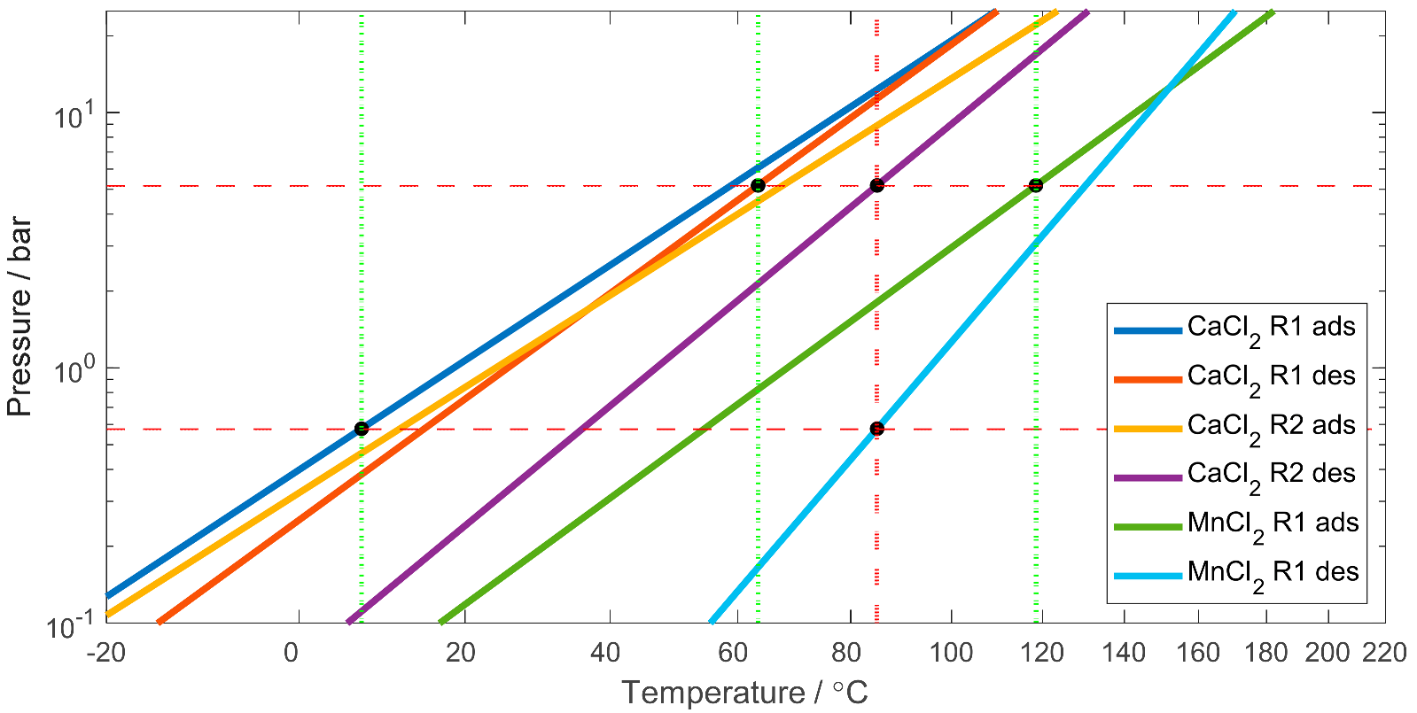
Clapeyron relationship plot for calcium chloride (8-4-2) and magnesium (6-2) pair, showing all lines. The adsorption line of the (4-2) reaction intersects the (8-4) reaction.
Figure A11.
Clapeyron relationship plot for calcium chloride (8-4-2) and magnesium (6-2) pair, showing all lines. The adsorption line of the (4-2) reaction intersects the (8-4) reaction.

Appendix J
Ramping simulations that provide basic evidence for deciding on sample dimensions before validation with an LTJ test. Simulated using empirical data equivalent to that in Figure 8.
Figure A12.
Simulation of 35 mm outer diameter disk over a 12.7 mm tube with rapid wall ramp in temperature.
Figure A12.
Simulation of 35 mm outer diameter disk over a 12.7 mm tube with rapid wall ramp in temperature.

Figure A13.
Simulation of 36 mm outer diameter disk over a 25.4 mm tube with rapid wall rapid change in temperature.
Figure A13.
Simulation of 36 mm outer diameter disk over a 25.4 mm tube with rapid wall rapid change in temperature.

Appendix K

Table A1.
COP evaluations for different sizes, all cases are manganese chloride (6–2) and calcium chloride (–4) pair at 85 °C waste heat temperature, with the equilibrium data from the LTJ. * final selected sizing.
Table A1.
COP evaluations for different sizes, all cases are manganese chloride (6–2) and calcium chloride (–4) pair at 85 °C waste heat temperature, with the equilibrium data from the LTJ. * final selected sizing.
| Index | Tube OD (Cell ID mm) | Composite OD (mm) | COP | Volume of Composite (m3) |
|---|---|---|---|---|
| (a) | 25.4 (1”) | 36 | 0.197 | 0.00051 |
| (b) | 25.4 (1”) | 40 | 0.238 | 0.00075 |
| (c) | 19.05 (3/4”) | 36 | 0.293 | 0.00073 |
| (d) | 19.05 (3/4”) | 40 | 0.317 | 0.00097 |
| (e) | 12.7 (1/2”) | 33.6 * | 0.356 | 0.00076 |
References
- BEIS. UK Hydrogen Strategy. 2021. Available online: https://assets.publishing.service.gov.uk/government/uploads/system/uploads/attachment_data/file/1011283/UK-Hydrogen-Strategy_web.pdf (accessed on 5 March 2022).
- Hinmers, S.; Critoph, R.E. Modelling the Ammoniation of Barium Chloride for Chemical Heat Transformations. Energies 2019, 12, 4404. [Google Scholar] [CrossRef] [Green Version]
- Atkinson, G.H.; Hinmers, S.; Critoph, R.E.; van der Pal, M. Ammonium Chloride (NH4Cl)—Ammonia (NH3): Sorption Characteristics for Heat Pump Applications. Energies 2021, 14, 6002. [Google Scholar] [CrossRef]
- Vasiliev, L.; Mishkinis, D.; Antukh, A.; Kulakov, A. Resorption heat pump. Appl. Therm. Eng. 2004, 24, 1893–1903. [Google Scholar] [CrossRef]
- Bao, H.; Wang, R.; Oliveira, R.; Li, T. Resorption system for cold storage and long-distance refrigeration. Appl. Energy 2012, 93, 479–487. [Google Scholar] [CrossRef]
- Goetz, V.; Elie, F.; Spinner, B. The structure and performance of single effect solid-gas chemical heat pumps. Heat Recover. Syst. CHP 1993, 13, 79–96. [Google Scholar] [CrossRef]
- Cudok, F.; Giannetti, N.; Ciganda, J.L.C.; Aoyama, J.; Babu, P.; Coronas, A.; Fujii, T.; Inoue, N.; Saito, K.; Yamaguchi, S.; et al. Absorption heat transformer-state-of-the-art of industrial applications. Renew. Sustain. Energy Rev. 2021, 141, 110757. [Google Scholar] [CrossRef]
- Metcalf, S.; Critoph, R.; Tamainot-Telto, Z. Optimal cycle selection in carbon-ammonia adsorption cycles. Int. J. Refrig. 2012, 35, 571–580. [Google Scholar] [CrossRef]
- Korhammer, K.; Neumann, K.; Opel, O.; Ruck, W.K. Micro-scale Thermodynamic and Kinetic Analysis of a Calcium Chloride Methanol System for Process Cooling. Energy Procedia 2017, 105, 4363–4369. [Google Scholar] [CrossRef]
- Offenhartz, P.O.; Rye, T.; Malsberber; Schwartz, D. Methanol-Based Heat Pump for Solar Heating, Cooling and Storage, Phase III; EIC Laboratories, Inc.: Newton, MA, USA, 1981. [Google Scholar]
- Aristov, Y. Optimal adsorbent for adsorptive heat transformers: Dynamic considerations. Int. J. Refrig. 2009, 32, 675–686. [Google Scholar] [CrossRef]
- Critoph, R. Activated carbon adsorption cycles for refrigeration and heat pumping. Carbon 1989, 27, 63–70. [Google Scholar] [CrossRef]
- van der Pal, M.; Critoph, R.E. Performance of CaCl2-reactor for application in ammonia-salt based thermal transformers. Appl. Therm. Eng. 2017, 126, 518–524. [Google Scholar] [CrossRef]
- Neveu, P.; Castaing, J. Solid-gas chemical heat pumps: Field of application and performance of the internal heat of reaction recovery process. Heat Recover. Syst. CHP 1993, 13, 233–251. [Google Scholar] [CrossRef]
- Moundanga-Iniamy, M.; Touzain, P. The Reaction between Ammonia and Magnesium Chloride Graphite Intercalation Compounds. Mater. Sci. Forum 1992, 91–93, 823–828. [Google Scholar] [CrossRef]
- Touzain, P.; Moundanga-Iniamy, M. Thermochemical Heat Transformation: Study of The Ammonia/Magnesium Chloride-Gic Pair in A Laboratory Pilot. Mol. Cryst. Liq. Cryst. Sci. Technol. Sect. A Mol. Cryst. Liq. Cryst. 1994, 245, 243–248. [Google Scholar] [CrossRef]
- Touzain, P.; El Atifi, A.; Moundanga-Iniamy, M. Reaction of Metal Chloride Graphite Intercalation Compounds with Ammonia. Mol. Cryst. Liq. Cryst. Sci. Technol. Sect. A Mol. Cryst. Liq. Cryst. 1994, 245, 231–236. [Google Scholar] [CrossRef]
- Mazet, N.; Amouroux, M.; Spinner, B. Analysis and Experimental Study of the Transformation of a Non-Isothermal Solid/Gas Reacting Medium. Chem. Eng. Commun. 1991, 99, 155–174. [Google Scholar] [CrossRef]
- Mazet, N.; Amouroux, M. Analysis of Heat Transfer in a Non-Isothermal Solid-Gas Reacting Medium. Chem. Eng. Commun. 1991, 99, 175–200. [Google Scholar] [CrossRef]
- Zhong, Y.; Critoph, R.; Thorpe, R.; Tamainot-Telto, Z. Dynamics of BaCl2–NH3 adsorption pair. Appl. Therm. Eng. 2009, 29, 1180–1186. [Google Scholar] [CrossRef] [Green Version]
- An, G.; Wang, L.; Zhang, Y. Overall evaluation of single- and multi-halide composites for multi-mode thermal-energy storage. Energy 2020, 212, 118756. [Google Scholar] [CrossRef]
- An, G.; Li, Y.; Wang, L.; Gao, J. Wide applicability of analogical models coupled with hysteresis effect for halide/ammonia working pairs. Chem. Eng. J. 2020, 394, 125020. [Google Scholar] [CrossRef]
- Zhong, Y.; Critoph, R.; Thorpe, R.; Tamainot-Telto, Z.; Aristov, Y. Isothermal sorption characteristics of the BaCl2–NH3 pair in a vermiculite host matrix. Appl. Therm. Eng. 2007, 27, 2455–2462. [Google Scholar] [CrossRef]
- Dawoud, B.; Aristov, Y. Experimental study on the kinetics of water vapor sorption on selective water sorbents, silica gel and alumina under typical operating conditions of sorption heat pumps. Int. J. Heat Mass Transf. 2003, 46, 273–281. [Google Scholar] [CrossRef]
- Veselovskaya, J.V.; Tokarev, M.M. Novel ammonia sorbents “porous matrix modified by active salt” for adsorptive heat transformation: 4. Dynamics of quasi-isobaric ammonia sorption and desorption on BaCl2/vermiculite. Appl. Therm. Eng. 2011, 31, 566–572. [Google Scholar] [CrossRef]
- Aristov, Y.I. Experimental and numerical study of adsorptive chiller dynamics: Loose grains configuration. Appl. Therm. Eng. 2013, 61, 841–847. [Google Scholar] [CrossRef]
- Metcalf, S.; Rivero-Pacho, A.; Critoph, R. Design and Large Temperature Jump Testing of a Modular Finned-Tube Carbon–Ammonia Adsorption Generator for Gas-Fired Heat Pumps. Energies 2021, 14, 3332. [Google Scholar] [CrossRef]
- Sharma, R.; Kumar, E.A.; Dutta, P.; Murthy, S.S.; Aristov, Y.; Tokrev, M.; Li, T.; Wang, R. Ammoniated salt based solid sorption thermal batteries: A comparative study. Appl. Therm. Eng. 2021, 191, 116875. [Google Scholar] [CrossRef]
- Hinmers, S.; Atkinson, G.; Critoph, R.; van der Pal, M. Modelling and Analysis of Ammonia Sorption Reactions in Halide Salts. Int. J. Refrig. 2022. [Google Scholar] [CrossRef]
- An, G.; Wang, L.; Gao, J.; Wang, R. A review on the solid sorption mechanism and kinetic models of metal halide-ammonia working pairs. Renew. Sustain. Energy Rev. 2018, 91, 783–792. [Google Scholar] [CrossRef]
- Veselovskaya, J.; Critoph, R.; Thorpe, R.; Metcalf, S.; Tokarev, M.; Aristov, Y. Novel ammonia sorbents “porous matrix modified by active salt” for adsorptive heat transformation: 3. Testing of “BaCl2/vermiculite” composite in a lab-scale adsorption chiller. Appl. Therm. Eng. 2010, 30, 1188–1192. [Google Scholar] [CrossRef]
- Veselovskaya, J.V.; Tokarev, M.M.; Grekova, A.D.; Gordeeva, L.G. Novel ammonia sorbents ‘‘porous matrix modified by active salt” for adsorptive heat transformation: 6. The ways of adsorption dynamics enhancement. Appl. Therm. Eng. 2012, 37 (Suppl. C), 87–94. [Google Scholar] [CrossRef]
- Lebrun, M.; Spinner, B. Models of heat and mass transfers in solid—gas reactors used as chemical heat pumps. Chem. Eng. Sci. 1990, 45, 1743–1753. [Google Scholar] [CrossRef]
- Lebrun, M.; Spinner, B. Simulation for the development of solid—gas chemical heat pump pilot plants Part I. simulation and dimensioning. Chem. Eng. Process. Process Intensif. 1990, 28, 55–66. [Google Scholar] [CrossRef]
- Lebrun, M. Simulation for the development of solid—gas chemical heat pump pilot plants Part II. simulation and optimization of Discontinuous and pseudo-continuous operating cycles. Chem. Eng. Process. Process Intensif. 1990, 28, 67–77. [Google Scholar] [CrossRef]
- Levenspiel, O. Chemical Reaction Engineering, 3rd ed.; John Wiley & Sons: New York, NY, USA, 1999. [Google Scholar]
- Lu, H.-B.; Mazet, N.; Spinner, B. Modelling of gas-solid reaction—Coupling of heat and mass transfer with chemical reaction. Chem. Eng. Sci. 1996, 51, 3829–3845. [Google Scholar] [CrossRef]
- Lu, H.-B.; Mazet, N.; Coudevylle, O.; Mauran, S. Comparison of a general model with a simplified approach for the transformation of solid-gas media used in chemical heat transformers. Chem. Eng. Sci. 1997, 52, 311–327. [Google Scholar] [CrossRef]
- Lepinasse, E.; Goetz, V.; Crosat, G. Modelling and experimental investigation of a new type of thermochemical transformer based on the coupling of two solid-gas reactions. Chem. Eng. Process. Process Intensif. 1994, 33, 125–134. [Google Scholar] [CrossRef]
- Gluesenkamp, K.R.; Frazzica, A.; Velte, A.; Metcalf, S.; Yang, Z.; Rouhani, M.; Blackman, C.; Qu, M.; Laurenz, E.; Rivero-Pacho, A.; et al. Experimentally Measured Thermal Masses of Adsorption Heat Exchangers. Energies 2020, 13, 1150. [Google Scholar] [CrossRef] [Green Version]
Figure 1.
Simplified resorption machine, at low- and high-pressure phases of operation.

Figure 2.
Resorption machine Clapeyron diagram.

Figure 3.
Calcium chloride LTJ result at around 7 bar, the ammoniate phase changes can be seen: first 8–4 and then 4–2; 2–4 and 4–8 reactions follow after around 370 s. ENG denotes the salt-ENG composite. Pressure is plotted on the right-hand scale.
Figure 3.
Calcium chloride LTJ result at around 7 bar, the ammoniate phase changes can be seen: first 8–4 and then 4–2; 2–4 and 4–8 reactions follow after around 370 s. ENG denotes the salt-ENG composite. Pressure is plotted on the right-hand scale.

Figure 4.
Calcium chloride LTJ result at around 4 bar. In adsorption, the first cycle shows the subcooling effect and the returning to the phase change temperature of the 8–4 reaction; the second cycle under the same conditions instead appears to show a single phase change. Exp V is expansion vessel central temperature, Exp V Wall is expansion vessel wall temperature, and ENG is the ENG/composite temperature. Pressure is recorded against the right-hand axis.

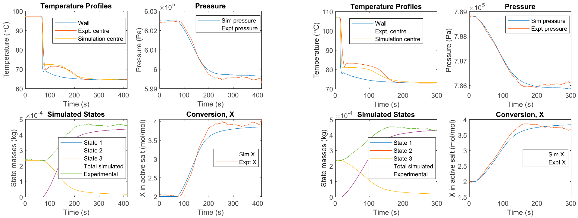
Figure 5.
Calcium chloride simulation results: (a) shows desorption over the two states, both isothermal changes can be seen; (b) shows the reverse cycle of adsorption.
Figure 5.
Calcium chloride simulation results: (a) shows desorption over the two states, both isothermal changes can be seen; (b) shows the reverse cycle of adsorption.

Figure 6.
Figure of a unit cell of a resorption generator: the central cylinder is water (heat transfer fluid), the middle grey tube is stainless steel, and the outer ring is ENG-salt composite. Key to assessing performance is the ratio of component diameters.
Figure 6.
Figure of a unit cell of a resorption generator: the central cylinder is water (heat transfer fluid), the middle grey tube is stainless steel, and the outer ring is ENG-salt composite. Key to assessing performance is the ratio of component diameters.

Figure 7.
Clapeyron diagrams for resorption pairs with hysteresis: (a) is calcium chloride (8-4) and magnesium (6-2) pair; (b) is the barium chloride (8-0) and calcium chloride (4-2) pair; (c) is calcium chloride (8-4-2) and magnesium (6-2) pair. Only the desorption line of the (4-2) calcium chloride reaction is shown for clarity; a plot including it can be seen in Appendix I.

Figure 8.
Shell side LTJ test for barium chloride and SMP plotted versus time. The peak value of SMP was 0.24 kW/L. The sample had a 35 mm outer diameter and was fitted over a 12.7 mm tube.
Figure 8.
Shell side LTJ test for barium chloride and SMP plotted versus time. The peak value of SMP was 0.24 kW/L. The sample had a 35 mm outer diameter and was fitted over a 12.7 mm tube.

Figure 9.
Heat transfer improvements: (a) shows a machined ‘bullet’ to enable a tighter fit of sample to be pushed over the tube, with the salt composite shown on the tube; (b) shows hexagonal samples inside the shell side LTJ, CALGAVIN insert can be seen within the tube.
Figure 9.
Heat transfer improvements: (a) shows a machined ‘bullet’ to enable a tighter fit of sample to be pushed over the tube, with the salt composite shown on the tube; (b) shows hexagonal samples inside the shell side LTJ, CALGAVIN insert can be seen within the tube.

Figure 10.
Result and simulation plot, and then SMP plot against time for 32 mm hexagonal sample of barium chloride. The simulation can be seen from a result by Hinmers et al. [29]. The initial spike in SMP is prior to the reaction occurring, the peak SMP ≈ 1.4 kW/L.
Figure 10.
Result and simulation plot, and then SMP plot against time for 32 mm hexagonal sample of barium chloride. The simulation can be seen from a result by Hinmers et al. [29]. The initial spike in SMP is prior to the reaction occurring, the peak SMP ≈ 1.4 kW/L.

Figure 11.
Engineering drawing of cross section of reactor, 3D form of reactor end with spot fitted ring.
Figure 11.
Engineering drawing of cross section of reactor, 3D form of reactor end with spot fitted ring.

Figure 12.
Reactor sizing and cutaway, distribution manifolds on the end. The longitudinal cutaway is shown from point B to B; it dissects the centre hexagonal sample. A cross section and end view are also shown. All measurements in mm.
Figure 12.
Reactor sizing and cutaway, distribution manifolds on the end. The longitudinal cutaway is shown from point B to B; it dissects the centre hexagonal sample. A cross section and end view are also shown. All measurements in mm.

Table 1.
Measured values for the Clapeyron relation for the onset of adsorption and desorption reactions, and the heat of reaction from tests with low hysteresis.
Table 1.
Measured values for the Clapeyron relation for the onset of adsorption and desorption reactions, and the heat of reaction from tests with low hysteresis.
| Salt | BaCl2 | CaCl2 | MnCl2 | |
|---|---|---|---|---|
| NH3 mole change | 8-0 | 8-4 | 4-2 | 6-2 |
| (J/kmol) | 48,924,790 | 36,365,790 | 41,202,320 | 58,196,253 |
| (J/kmol) | 37,360,200 | 32,844,620 | 31,699,720 | 36,611,107 |
| (J/kmol K) | 263,993 | 217,432 | 224,432 | 253,641 |
| (J/kmol K) | 229,454 | 208,302 | 202,390 | 202,865 |
| (J/kmol) | 40,745,437 | 42,080,324 | 39,948,772 | 42,523,900 |
| Reference | [29] | (This paper) | [29] | |
Table 2.
Constants for kinetic reaction models for the relevant salts reacting with ammonia.
| Salt | MnCl2 | BaCl2 | CaCl2 | CaCl2 |
|---|---|---|---|---|
| NH3 mole change | 6–2 | 8–0 | 8–4 | 4–2 |
| adsorption | 2 | 2 | 2 | 2 |
| adsorption | 3 | 0.1 | 1.5 | 3 |
| desorption | 3 | 2 | 2 | 1.5 |
| desorption | 3 | 3 | 3 | 2.5 |
| Active fraction | 0.8 | 0.78 | 0.8 | 0.8 |
| Source | [29] | [29] | (This paper) | (This paper) |
Table 3.
COP estimate for resorption pairs, values are estimated based on 33.6 mm outer diameter circular samples for the unit cell in Figure 8, neglecting any shell material.
Table 3.
COP estimate for resorption pairs, values are estimated based on 33.6 mm outer diameter circular samples for the unit cell in Figure 8, neglecting any shell material.
| Sorption Pair (mols NH3 Reacting) | Corresponding Diagram Figure 9 | COP |
|---|---|---|
| Calcium chloride (8-4) + Magnesium chloride (6-2) | (a) | 0.20 |
| Barium chloride (8-0) + Calcium chloride (4-2) | (b) | 0.34 |
| Calcium chloride (8-4-2) + Magnesium chloride (6-2) | (c) | 0.36 |
Table 4.
Number of discs (hexagon with 16 mm apothem) calculated based on barium result for SMP, and stoichiometry and uptake data. Disc numbers are rounded the nearest whole disc.
Table 4.
Number of discs (hexagon with 16 mm apothem) calculated based on barium result for SMP, and stoichiometry and uptake data. Disc numbers are rounded the nearest whole disc.
| Salt | Number of Discs | Number of Discs per Tube | Mass of Salt (kg) | Moles of Salt (kmol) | Stoichiometric Reaction Ratio |
|---|---|---|---|---|---|
| BaCl2 * | 509 | 73 | 0.787339 | 0.003781 | 8 |
| CaCl2 (4-2) | 1266 | 181 | 1.678507 | 0.015124 | 2 |
| CaCl2 (8-4) | 633 | 90 | 0.839254 | 0.007562 | 4 |
| CaCl2 (8-4-2) | 422 | 60 | 0.559502 | 0.005041 | 6 |
| MnCl2 | 501 | 72 | 0.951628 | 0.007562 | 4 |
* basis calculation from which the rest are determined.
Publisher’s Note: MDPI stays neutral with regard to jurisdictional claims in published maps and institutional affiliations. |
© 2022 by the authors. Licensee MDPI, Basel, Switzerland. This article is an open access article distributed under the terms and conditions of the Creative Commons Attribution (CC BY) license (https://creativecommons.org/licenses/by/4.0/).
Share and Cite
MDPI and ACS Style
Hinmers, S.; Atkinson, G.H.; Critoph, R.E.; van der Pal, M. Resorption Thermal Transformer Generator Design. Energies 2022, 15, 2058. https://0-doi-org.brum.beds.ac.uk/10.3390/en15062058
AMA Style
Hinmers S, Atkinson GH, Critoph RE, van der Pal M. Resorption Thermal Transformer Generator Design. Energies. 2022; 15(6):2058. https://0-doi-org.brum.beds.ac.uk/10.3390/en15062058
Chicago/Turabian StyleHinmers, Samuel, George H. Atkinson, Robert E. Critoph, and Michel van der Pal. 2022. "Resorption Thermal Transformer Generator Design" Energies 15, no. 6: 2058. https://0-doi-org.brum.beds.ac.uk/10.3390/en15062058
Note that from the first issue of 2016, this journal uses article numbers instead of page numbers. See further details here.