
Automated Detection of Electric Energy Consumption Load Profile Patterns


1
Sustainability and Energy Efficiency Area, Fundación Valenciaport, Building III, Avda. Muelle del Túria s/n, 46023 Valencia, Spain
2
Instituto Universitario de Automática e Informática Industrial, Universitat Politècnica de València, Camino de Vera s/n, 46023 Valencia, Spain
*
Author to whom correspondence should be addressed.
Energies 2022, 15(6), 2176; https://0-doi-org.brum.beds.ac.uk/10.3390/en15062176
Submission received: 17 January 2022
/
Revised: 21 February 2022
/
Accepted: 14 March 2022
/
Published: 16 March 2022
(This article belongs to the Special Issue Planning, Modelling, Operation and Assessment of Renewable Energy Power Systems)
Abstract
:Load profiles of energy consumption from smart meters are becoming more and more available, and the amount of data to analyse is huge. In order to automate this analysis, the application of state-of-the-art data mining techniques for time series analysis is reviewed. In particular, the use of dynamic clustering techniques to obtain and visualise temporal patterns characterising the users of electrical energy is deeply studied. The performed review can be used as a guide for those interested in the automatic analysis and groups of behaviour detection within load profile databases. Additionally, a selection of dynamic clustering algorithms have been implemented and the performances compared using an available electric energy consumption load profile database. The results allow experts to easily evaluate how users consume energy, to assess trends and to predict future scenarios.
1. Introduction
The electricity sector liberalisation process led to investments both in improving existing measurement and communications infrastructure, and taking the measurement and actuation capacity to a more significant number of points in medium and low voltage networks. Therefore, the availability of data that informs about the state of the network is increasingly higher and more complete. All these systems are part of the so-called Smart Grids, or intelligent networks of the future, a future which is not so far. An important source of information comes from the energy consumption of customers, measured regularly (every hour, half hour or quarter hour) and sent to the Distribution System Operators from the Smart Meters making use of Advanced Metering Infrastructure (AMI). In this way, there is an increasing amount of information on the energy consumption of customers, being stored in Big Data systems. This growing source of information demands specialised data mining techniques which can take benefit from it, extracting automatically helpful and summarised knowledge.
Data mining techniques have been described as the intermediate step within a bigger process, called Knowledge Discovery in Databases or KDD, described as “the nontrivial process of identifying valid, novel, potentially useful and ultimately understandable patterns in data” [1]. This process covers the whole sequence of knowledge extraction in large datasets or, in recent years, in large amounts of data from the Internet of Things (IoT) [2] and from Big Data systems [3]. The KDD process comprehends the following steps [4]:
- Initially, the expert or data analyst studies the dataset and makes an assumption or states a hypothesis regarding the objective of the knowledge discovery process, or the model or relationship that may be found among the different variables or features of the data objects. The subsequent analysis of the data will be based on these initial hypotheses, which would at the end be validated upon the results obtained, or not. If the results are not satisfactory, the expert will perform new assumptions or hypotheses, therefore starting the KDD process again.
- Then, the data warehousing process [5] is performed. This step of the analysis comprises all the techniques and procedures to process erroneous or missing values in the data, filter noise, produce specific queries to access the data, and rearrange the information in the desired format to be analysed.
- Then, the selected data mining technique or techniques are applied, with the objective of extracting valuable relations or information from the data, in the form of patterns, models, association rules or other things.
- The next step is the visualisation of results, along with numerical and/or categorical indicators and information to help the expert to identify and evaluate the results.
- Finally, the expert has to perform an interpretation of the results. In this step, the expert will validate the initial hypothesis made concerning the underneath models or patterns able to summarize the data, obtain conclusions and extract knowledge from the results. In the case these results are not satisfactory, new hypotheses can be formulated, which will imply the need for further data mining analyses, therefore starting the KDD process again.
The KDD process makes use of many different algorithms and techniques from different research fields: Pattern recognition and classification, statistics, data visualisation, machine learning and artificial intelligence [6]. According to Mitra et al. [1], the issue that makes KDD different from other areas is that it is focused on knowledge discovery from large sets of data, including the overall process of “storage and accessing such data, scaling of algorithms to massive datasets, interpretation and visualisation of results, and the modelling and support of the overall human-machine interaction”. In recent years, the research field on KDD and data mining has started to move towards the analysis of data in Big Data systems using Big Data Analytics tools [7]. The objectives are kept the same, but the techniques have been adopted and have gone through an evolution process to be able to manage large amounts of unordered data from distributed sources, especially in the case of stream data mining, where the amount of available data per unit of time makes unavailable the traditional schema of loading the data and then performing a centralised analysis on them [7].
According to Mitra et al. [1], there are two main tasks performed by data mining algorithms: Descriptive and predictive tasks. The first deals with the description of the data, using patterns, for example, and the other with obtaining models that establish input–output relations among variables and predict future outcomes given the initial conditions and values of inputs. Beyond this division, further classifications can be given according to Han and Kamber [4], based on the type of data to be mined (and the type of database), and the specific objectives of the data mining process, or the kind of knowledge being mined. Regarding the types of databases, a detailed description can be found in the book by Han and Kamber [4] with the main types being: Relational, transactional, repositories, etc. Regarding the objectives of data mining, Han and Kamber group the techniques according to two main objectives: The static analysis of the data and the dynamic analysis of the data.
Static analysis includes all the techniques that aim to analyse data from a particular period, but without taking into account the temporal record in which the data were acquired as the objective of the analysis. The authors subdivide these techniques depending on the objective: Techniques for description and techniques for prediction. The description objective includes: The automated preparation of summaries of the resulting classes (summaries and class description); mining or obtaining frequent patterns (frequent pattern mining); the classification of objects clustering or segmentation analysis; and out-of-range data detection (outliers). As part of the prediction objective, the techniques included are: Association between variables, correlation and the development of prediction models, through regression, neural networks or other techniques.
Regarding dynamic analysis, the objective is to evaluate and analyse the trend of the data series, whether they are temporal or sequential. The same objectives described for the static analysis can also be applied to the dynamic case. However, it should be taken into account that the inclusion of the temporal dimension as an objective of the analysis may imply the modification of the techniques used in the static analysis, increasing its complexity (and its difficulty for an understandable visualisation of the results).
This work studies the application of state-of-the-art techniques for dynamic clustering of available databases of load profiles from Smart Meters energy consumption data. In particular, the use of data mining techniques to obtain and visualise temporal patterns characterising the users of electrical energy (grouping them according to these patterns in a small number of groups or clusters) is the main aim. This will allow the evaluation by experts of how users consume energy, both during the day and during a sequence of days, then it will be possible to assess trends and predict future scenarios.
The paper is structured as follows. First, a review is done about the most common clustering techniques (Section 2), describing both the most used similarity measures for static (Section 2.2), and dynamic (Section 2.3) data analysis. Secondly, the static clustering techniques (Section 3) are presented as an introduction. Then, the dynamic clustering techniques are further described (Section 4) in three subsections, taking into account the classification of the algorithms according to how the data are analysed: The direct analysis on the raw time series (Section 4.1), the analysis applied on a transformation of the original dataset (Section 4.2), and the analysis applied on the parameters of models obtained from the original data (Section 4.3). In Section 5, a set of these techniques is selected and applied to a database of hourly energy consumption values for a sample of residential customers, comparing the results among algorithms by defining quantitative indicators of validity and observing the resulting patterns (Section 5.2). Finally, Section 6 includes a summary with the main conclusions obtained. Table 1 summarises the notation used throughout this document.
2. Clustering Techniques
Clustering is the “unsupervised learning task whose objective is to decompose a set of objects into subsets or clusters, based on a measure of similarity” [8]. The resulting classes or clusters are therefore groups of objects according to a mathematical measure of similarity (the most similar objects are grouped together). From each resulting class, an object is usually obtained that is the pattern, prototype or characteristic object of the class, and represents all the objects that belong to that class. This object is called centroid, and it can be calculated as the mean value of all the objects that belong to the class, or by other formulations. Figure 1 presents an example of clustering into classes a set of objects with two dimensions or characteristics, and their corresponding centroids, calculated in this case as the center of gravity of each class.
However, before choosing a specific clustering algorithm, it is essential to perform some selections according to the type of data to be analysed. The decisions are related to the static or dynamic nature of the data, and how similarity between the data must be understood. Section 2.1–Section 2.3 will give hints concerning this previous selection.
2.1. Taxonomy of Clustering Techniques
Clustering algorithms can be classified according to different criteria:
- The dynamic nature of data and classes. This criterion classifies algorithms based on whether they are designed for dynamic or static data, and for a fixed or time-varying number of classes.
- The way the data are analysed. This criterion classifies the algorithms according to the strategy or technique they use to analyse the data, and specifically if they carry out an initial transformation of the same into another set of data on which they perform the analysis.
- The number of dimensions or characteristics of the data. This criterion classifies algorithms according to the number of dimensions of the data they analyse.
The first criterion, the dynamic nature of the data and the resulting classes, classifies the segmentation algorithms into four types, as can be seen in Table 2, described by Weber [8] and they are the following:
- The data, although they can be time series, are treated as static. The segmentation algorithms are therefore focused on static analysis. This is the case of the example shown in Figure 1.
- While they can be time series, the data are treated as static. The number of classes, however, is variable. This is the case when the database is partitioned and batch processed sequentially, as the example in Figure 2 indicates. With each batch the number of classes may vary, showing a variation in the trend of the data and its composition. Therefore, it is necessary to implement techniques that make a correspondence between the classes of one batch and the next [9], taking into account the possibility of the formation of new classes, the disappearance of classes that had been formed previously, the merge of two or more classes, and the separation of a class into smaller classes.
- The data is treated as dynamic, varying with time; therefore the objects become trajectories of each characteristic of the object or data. The number of classes is fixed. The resulting centroids are defined by the trajectories of their dimensions, which represent the evolution in time of the objects belonging to each class. An example of this segmentation analysis is shown in Figure 3.
- The data is treated as dynamic, varying over time, as in Type 3. The number of classes is not fixed, and can vary with each batch or cycle. Therefore, the same techniques for Type 2 must be taken into account. Figure 4 shows an example of this type of analysis.
In a simplified way, the clustering techniques can be divided into static (types 1 and 2) and dynamic (types 3 and 4); then the basic techniques for types 1 and 3 are defined, and they are applied repeatedly (in batches) for types 2 and 4. Thus, Section 2 focuses on type 1 static techniques for the analysis of data in a particular time period, but without considering the analysis of the time variable of the data. Section 2.3 presents type 3 dynamic analysis techniques to analyse time trends in data series, both batch or time continuous.
2.2. Similarity for Static Data
In order to select the most appropriate distance as a measure of similarity to compare two objects in a particular problem, the nature of the data and its characteristics or dimensions must be considered:
- If the objects include qualitative features or values selected from a list of categories, then previously described quantitative distances are not suitable to evaluate the similarity among the objects. In this case, a specific distance for qualitative data similarity must be used. For example, a measure can be used from the matching or coincident coefficient family of distances, which can only take two possible values (0 or 1) if the characteristics of both objects are coincident or not. Two of these distance measures are the simple matching coefficient [10], and the Jaccard distance [11].
- If all the characteristics or dimensions of the objects are quantitative or numerical, then quantitative similarity measures can be used, and the two more used are described next.
2.2.1. The Minkowski Metric
This measure of similarity for two objects and is described in (1), where d is the number of characteristics or dimensions of both objects, and r is a parameter that determines variants of this metric. The most known of these variants, defined in (2), is obtained when = 2, and is known as Euclidean distance. The Euclidean distance is the shortest distance among two points, and is one of the most used quantitative measures of similarity in literature clustering algorithms.
2.2.2. The Mahalanobis Distance
The Mahalanobis distance normalises each one of the data characteristics of the objects to zero mean and unity variance. In order to do so the distance (3) includes the covariance matrix of the objects (4) in the term .
If the case is given that is the identity matrix, then the result is the previously described square of the Euclidean distance.
2.2.3. Selection of a Suitable Distance Measure
Therefore, to compare numerical characteristics of objects, like in the case of energy consumption load profiles, one of the measures defined above (or any of the others described in the literature) can be used.
The choice can be made based on the scale of the values in the different dimensions. If all the characteristics of the objects have a similar order of magnitude, the Euclidean distance can be applied directly to the data without normalising. In contrast, the Mahalanobis distance including the matrix of covariances must be used to apply automatically a normalisation of the values in all the dimensions of the objects.
In any case, it is always recommended to normalise the data before analysing it. If normalising is not possible, there are distance measures that allow clustering data without normalisation, although its dimensions have very different orders of magnitude. In this case, clusters with various geometrical forms [12] are obtained: The Euclidean distance lead to hyperspherical clusters, the Mahalanobis distance hyperellipsoidal clusters, and adaptive norms (as those of the GK Gustafson-Kessel [13] algorithm) obtain clusters with varying forms but constant volume.
2.3. Similarity for Dynamic Data: Time Series Clustering
Next, the three more common similarity measures used in the literature for time series clustering are presented: The coefficient of correlation (Section 2.3.1), the DTW distance (Section 2.3.2), and the Kullback–Leibler distance (Section 2.3.3).
2.3.1. Correlation
The analysis of correlation gives a measure of linear relation among two series of data. The more common coefficient of correlation for comparing two series of data i and k of the same longitude p, is the coefficient Pearson of linear correlation, described in (5), where is the mean value of the series of data and s is the standard deviation of the corresponding series (6).
The correlation coefficient can take values between −1 and 1; 1 shows a perfect correlation between the two data series; −1 also indicates that the two objects are correlated, but his trend is reverse (if the value of an object increases, the value of the other is reduced in the same proportion). A coefficient of correlation 0 indicates that there is no correlation between the series of data, and therefore it can be said that both series are linearly independent.
2.3.2. Dynamic Time Warping
Dynamic Time Warping or DTW [14,15] is a technique used to compare two time series that can have different longitudes or sampling periods. DTW looks for the optimal correspondence between the two time series regarding this shape.
Given two time series, R and S, of length n and m, respectively, the matrix of distances is defined, where each element corresponds with the distance among and (calculated using the Euclidean distance, for example). It defines the warping path as a vector of distances among R and S that has to fulfil some conditions [16]:
- Delimitation: This condition establishes the principle and the end of the alignment in the vertices of the matrix , i.e., and .
- Continuity: Given and , then 1 and 1. This condition ensures that the elements of the alignment are adjacent.
- Monotonicity: Given and , then and , having to fulfil at least a strict inequality. This condition forces the alignment to advance towards the vertex of the matrix of distances.
The path of optimum alignment is the one that, fulfilling the previously described conditions, minimises the sum of the square distances for the complete path, as can be seen in (7).
This optimised sequence of distances can be obtained through the accumulated matrix D method [16], following the formulation in (8).
From this matrix D, the points of optimum alignment are obtained recursively, starting from the last point () and following the formulation described in (9).
2.3.3. Kullback–Leibler Distance
Given two distributions p and q in a series T, the relative entropy or distance of Kullback–Leibler [17] is defined as the divergence among two distributions of probability calculated using (10).
The Kullback–Leibler distance is used as a dissimilarity measure. In [18], for example, it is used as a measure of the increase in divergence that would be produced when two clusters are merged.
2.3.4. Other Similarity Measures for Dynamic Data
There are other distances used as similarity measures in the literature to compare time series, and also distances very specific to application can be developed like those presented in [19] or [20]. The work of [21] is a good review, and the authors present an empirical evaluation of seven groups of similarity measures applied to 45 different time series. In any case, the distance selection requires a previous analysis of the nature of the available data by following the same rules explained for static data (Section 2.2) with this initial. In both cases, as will be seen next, the distance is one of the main characteristics within the static (Section 3) or dynamic clustering (Section 4), together with the clustering algorithm and the optimisation techniques.
3. Clustering Algorithms for Static Analysis
While the aim of the paper is the use of dynamic clustering techniques for time series load profiles as dynamic data, most dynamic algorithms are briefly described next. Most clustering algorithms for static analysis described in the literature are variations or modifications of these two algorithms: The K-means and the FCM. A complete review of clustering algorithms for static data in the literature is presented in the works of [22] or [4].
3.1. K-Means
The K-means algorithm [23] is one of the first and more used clustering algorithms. Its name refers to the number k of classes to look for in the set of data, and it is an input parameter for the algorithm. The algorithm minimises the cost function defined in (11). This cost function is calculated as the sum of all the sums of the distances of the centroids of the classes to the objects that belong to them. Therefore, the lower these distances, the more compact the clusters, and the lower the value of the function of cost. The algorithm procedure to achieve this aim is as follows:
- Select c objects of the dataset, which will be the initial centroids. This selection influences the final result. Therefore, a suitable representation of the existing patterns must be done for the algorithm convergence to a global optimum [6]. In order to do so, a heuristic selection or based on previous knowledge of the patterns must be done, or algorithms adapted for the initial selection of prototypes can be used, such as the algorithm K-means ++ [24].
- Compute all the Euclidean distances of the remaining objects to the centroids, and assign each object to the cluster with a lower distance.
- Recompute centroids as the mean value of all the objects belonging to each class.
- Go back to step 2, until some ending condition is fulfilled, like achieving a maximum number of iterations, or that the value of the cost function does not vary above some predefined threshold between two consecutive iterations.
3.2. Fuzzy C-Means (FCM)
Bezdek and Dunn developed the FCM algorithm [25,26]. It applies fuzzy logic [27] to the K-means algorithm. The cost function defined in (11) is modified as presented in (12), so that the sum of distances is weighted by the fuzzy membership () of each object to each cluster subject to (13), i.e., the sum of all the fuzzy memberships of an object to all the clusters has to be 1.
The expression is a measure of similarity described in (14), where matrix B defines the geometry of the clusters. If B is the identity matrix, then the similarity measure is the Euclidean distance (2). In contrast, if B is the inverse of the objects covariance, then the result is the Mahalanobis distance (3).
The iterative minimisation of the objective function gives two formulas for centroids and fuzzy membership calculation described in (15) and (16). The procedure of the FCM algorithm is described next:
- Initialise fuzzy membership matrix U with random values.
- Calculate the centroids as described in (16).
- Calculate the distances of objects to the centroids of each class, according to the measure of similarity described in (14).
- Recompute fuzzy membership matrix U, according to (15).
- Go back to step 2, until some ending condition is fulfilled, like achieving a maximum number of iterations, or that the value of the fuzzy memberships do not vary above some predefined threshold between two consecutive iterations.
3.3. Selection of the Static Clustering Algorithm According to the Application
In general, the algorithm (or set of algorithms) to apply depends on the nature of the data to analyse. This previous study of the objects and their characteristics will lead to a good selection among the algorithms described in the literature, and the decision will depend on whether the employed similarity measure (distance) allows comparing the objects in the set of data. For example, in [12], the authors use fuzzy clustering algorithms for the identification of local models of non-linear processes. The algorithms implemented are the FCM, the GK, and other algorithms, like the AFCRC (Adaptive Fuzzy C-Regression models with Convexity enhancement) [28], which makes use of a weighted combination of distances including the minimisation of a prediction error of the model. In [29], the authors present a clustering algorithm for the online identification of fuzzy models. The algorithm is called the Method of Evolutionary–Agglomerative Clustering, and the Euclidean distance is used for each step of the incremental clustering every time new data are available for the analysis, and allowing merging and eliminating clusters.
The authors [30] use the K-means algorithm over an SOM (Self-Organizing Map) [31] classification of profiles of energetic consumption of 24 daily values in a sample of domestic clients. In this case, all the dimensions present the same scale (energy data with the same order of magnitude), and therefore the Euclidean distance can be applied as a measure of similarity to clusters concerningthe spatial distribution given by theSOM net.
In [32], K-means is applied on a set of quantitative indicators weighted by importance to detect possible sources of water pollution. Jeong, H. et al. [33] uses K-means clustering on load profiles of residential customers in combination with extreme points and demographic characteristics. On the other hand, in [34] presents a fuzzy clustering algorithm based in the Fuzzy K-Partition [35] that employs a specific measure to make possible the clustering of categorical or qualitative data.
For the analysis of visual information, the authors [36], for example, apply the MeanShift algorithm clustering [37] to identify and group three-dimensional objects of a cloud of points obtained by a LIDAR (Laser Imaging Detection and Ranging) sensor. The algorithm MeanShift clusters the objects according to probability density functions that explain the set of data. In [38] the Multi-Objective Fast Generalized Fuzzy C-Means or MOFGFCM clustering is used to analyse SAR (Synthetic Aperture Radar) images. This algorithm optimises two cost functions specifically defined for the analysis of images: The FGFCM algorithm [39] and the Xie-Beni or XB [40] index.
4. Clustering Algorithms for Dynamic Analysis
In this section, clustering algorithms with the aim of dynamic analysis of the data are presented, including among them time series data. These techniques are more complex than those presented in the previous section, although they are based on them, and the understandable visualisation of the results is much more difficult in this case.
Dynamic techniques can be classified depending on the number of characteristics or dimensions of the objects, and algorithms are typically classified into two types: Those that make segmentation of objects of only one dimension (like the values of an electrocardiogram), and those that make segmentation in objects of n dimensions. A more suitable classification of the algorithms is based on how the data are processed. Liao [41] detects three different methods of analysis in the clustering algorithms for dynamic analysis: Process the time series in its original form, transform the data into a reduced representation according to its characteristics and clustering, or obtain models that represent the data prior to the segmentation.
Next, the literature algorithms are described according to the way that the data are processed. Nevertheless, in the description of the algorithms this classification is also included according to the dynamic nature of the data and the clusters, and whether the algorithm is designed for data of one dimension or more. The following information has been extracted from previous reviews made by several authors, such as [41,42,43,44].
4.1. Raw Time Series Data Clustering
The algorithms that perform the clustering of the time series in its original (raw) form are in most cases modifications of an equivalent algorithm for static analysis, where the similarity measure is substituted by a distance suitable to compare two series on the data.
The first developments were done in the decade of 1990. In [45] the Ward Generalised criterion [46] was used to develop a procedure of cluster reorganization for the time where, from an initial partition, the objects were reassigned to the clusters in each iteration applying a measure of similarity by minimising the Ward function (, with p being a function representing the objects’ adequacy concerning the clusters they belong to). This process is repeated for all the characteristics or dimensions of the objects at each iteration, having therefore a matrix of similarity measures and obtaining a global value of similarity as the weighted sum of all matrix values. Other authors have used this approach [47] but applying other clustering techniques (for example, K-means, FCM or genetic algorithms) to analyse multivariable time series with different lengths.
In [48] modified FCM is presented where the correlation Pearson is used as a similarity measure to compare fMRI (functional images of magnetic resonance) time series. On the other hand, [49] uses two similarity measures (the distance Kullback–Leibler and the Chernoff measure) to classify time series with different patterns.
In [50] hierarchical clustering is applied to identify patterns and trends in different time periods (days, weeks, seasons) in one-dimensional time series, and it is applied to a laboratory energy consumption. The Euclidean distance is used to calculate similarities among load profiles and classify them into clusters.
The authors [51] develop a similarity measure to be used in the case of time series with noise. The measure is based on the seasonality concept: A normalised load profile is defined for each cluster as a function of the date (along the year) after deleting any external factors other than those that can influence the data evolution. The result is a distance equivalent to a weighted Euclidean distance where elements with high standard deviation have less importance in the calculation of the distance.
Other authors propose developing specific algorithms for time series clustering. In [52], for example, Vector Quantization (VQ) is presented for obtaining clusters in data fRMI. The algorithm, similar to SOM (Self-Organizing Map), gets representative patterns of the evolution of the data in greyscale.
In [53], the Computational Verb Theory [54] is used for stock market time series. The authors define three computational verbs: Increase, decrease and remain. The clustering algorithm calculates the distances among the series of data and these three verbs, and then makes the clustering.
In [55], the STS Short Time Series distance is used as a similarity measure to catch differences in the shape of time series. The authors develop the FSTS (fuzzy short time series) algorithm by modifying FCM with STS distance. This distance is defined as the square difference of the slopes of two time series in an interval of temporary series, and it is, therefore, a measure of the rate of change in the evolution of both time series.
In [56], a two-step clustering method is proposed. In the first step, multivariable data are converted into one-dimensional time series by applying a static clustering algorithm, like the K-means. This result is somehow similar to state variables of a process. In the second step, the clustering algorithm is applied again to cluster the variables in several classes. In the first step, the author uses the Euclidean distance, and, in the second step, different similarity measures are used, like DTW or the Kullback–Leibler distance [41].
Moreover, for the case of Type 3 clustering algorithms described in Table 2, Weber [8] describes the algorithm called FFCM or Functional Fuzzy C-Means. This algorithm is presented as a generalisation of FCM for the dynamic analysis. In the algorithm, the distance d between two trajectories, f and g, is computed as follows:
- Define the fuzzy membership function “almost zero” . This membership function is symmetric, and achieves the maximum value of 1 when x equals zero. The form of the function can vary, although Weber defines a Gaussian function whose value rapidly decreases as the value of x increases.
- Compute the similarity function between two trajectories f and g, as the fuzzification of the difference between them, i.e., .
- Compute the distance between the two trajectories f and g as the inverse of the similarity, i.e., 1.
The FFCM algorithm calculates the membership of an object i to a class j for each iteration using (17), where represents the feature vector of the object i, and and are the centroids of the classes j and k, respectively.
In the description of the algorithm FFCM, Weber indicates that, if the trajectories are defined as sets of series of real values, a numerical distance can be applied, like the Euclidean distance, substituting, therefore, the operator of distance d.
Some interesting works for raw data analysis are those that present developments that look for a better interpretation of the time evolution of the identified patterns. For example, Meesrikamolkul et al. [57] propose a modified K-means clustering algorithm for time series, the Shape-Based Clustering, where the Euclidean distance is replaced by a Dynamic Time Warping (DTW) alignment between time series. Since the computational cost of the DTW is high, the authors present a method to obtain the representative element from each cluster called Ranking Shape-based Template Matching Framework (RSTMF), which can average a group of time series effectively but take as much as 400 times less computational time than that of a previous method called STMF (Shape-based Template Matching Framework).
In [58], the authors present a modification of the FCM algorithm for time series data, defining the key points in a time series as the group of points that describe, implicitly, how a series changes at a particular time. These points usually represent specific events, such as the start or the end in a tendency of upward or downward, the peak or the bottom of the series. The key points reveal the dynamic aspect of a given time series. The authors present a study of the dynamic switching of the time series among a fixed number of clusters, over time, based on the membership coefficient at each step.
In [59], the authors present a clustering algorithm for clustering spatio-temporal data where the Euclidean distance is replaced by an augmented distance, which is the weighted sum of two Euclidean distances: The comparison of the spatial components, and the comparison of the temporal features. This modification is later extended in [60] to n features or dimensions with the concept of blocks or groups of similar features, computing a weighted sum of Euclidean distances where the different weights are obtained by Particle Swarm Optimisation (PSO) [61].
A new modification is presented in [62], where the algorithms FCM, Fuzzy C-Medoids [63], and a third hybrid technique that uses both, are modified, and a DTW distance is used as the similarity measure to cluster one-dimensional time series data. The authors indicate that the use of the DTW is appropriate only in those cases when the similarity is sought between the shapes of the data objects, and depending on the nature of the data themselves.
Finally, Benítez, I. [64] proposes a framework where different static clustering techniques can be employed for dynamic analysis using the modification/substitution of the similarity measures by others, then allowing comparison between time series. The aim is to obtain clusters (and prototypes) showing the evolution of the data dimensions along time.
4.2. Feature-Based Time Series Data Clustering
As stated by Fu, T.C. [44], one of the objectives of time series processing is the transformation of the data to a reduced dimensionality or a summary or reduced amount of representative values before the clustering process.
In this sense, Wilpon, J. et al. [65] obtains clusters of spoken sentences by the combination of word patterns. The clusters evolve, combining different patterns. Different techniques to get the cluster centers such as minmax computation or averaging, are presented. A modified K-means algorithm is presented, where the similarity between time series is computed applying the log-likelihood distance proposed by Itakura [66], based on autocorrelation coefficients.
In [67], the authors perform clustering on vibration sensor time measures from industrial machine tools to serve as a predictive maintenance diagnosis. First, the time transients are identified from the raw data, by comparison with regular use steady state patterns. Then, this information is used to compute Self Organizing Feature Maps (SOFM).
Ref. [68] performs feature-based clustering on fMRI data, based on the cross-correlation function, presented in a previous work in [69]. The raw data are reduced in size by a selection process of only relevant data from the magnetic resonance that can be representative to form the different clusters. Cross-correlation is applied between the fMRI data and a function defined as the “excitation paradigm”. The resulting correlation indices are used for the clustering process, along with features or indices such as the strength of activation or the response delay.
Ref. [70] compresses the input patterns by a perceptually important point (PIP) identification algorithm, replacing the original data by a group of PIPs, thus reducing dimensionality. Then, the authors identify patterns making use of SOM applied to data sequences segmented by a sliding window, to mine frequent patterns in the temporal series.
The work in [71] applies dimensionality reduction on the time series data making use of the Haar wavelet transform. The authors present a modified incremental K-means clustering, where the Haar wavelet is applied to the data, and the centers from the clustering results are used as inputs for another clustering at a more satisfactory resolution level, proceeding this way until the termination criterion is met. The same approach, although with different techniques, is presented in the work of [72]: An incremental clustering for time series is shown, based on the identification of the Longest Common Subpaths (LCSS) from dimensionality reduced time series picked randomly. Then, a fuzzy clustering, such as the FCM, is applied, to create new classes dynamically, modify existing ones, and/or remove unchanged clusters. Ref. [73] finds groups in commercial and industrial weekly load patterns for long-term energy planning with a similar wavelet approach.
In [74], the multi-solution piecewise aggregate approximation (MPAA) transform is presented. The technique is an iterative segmentation of a time series in lower dimension sequences of the average values. In each level of dimensionality reduction, K-means clustering is applied, and the intra-cluster error is compared with the Hoeffding bound [75], as a stopping condition. The clustering algorithm is then used in this work for data stream clustering, by applying the nearest neighbour assignment of new incoming sequences to existing clusters, and then re-computing the MPAA clustering process only on the affected cluster.
The authors [76] propose clustering time series using kernel density-based clustering. The kernel-based clustering method comprises two parts: A nonlinear transformation that maps data points from a low-dimensional input space to a high-dimensional feature space induced by an inner product kernel or a Mercer kernel, and a learning algorithm to find linear patterns in that feature space. The use of a density-based clustering algorithm, such as DBSCAN (Density-Based Spatial Clustering of Applications with Noise) [77] avoids defining the number of clusters to be found as an input parameter. Ref. [78] performs a dimensionality reduction of the raw time series data by applying the Independent Component Analysis (ICA), a statistical method similar to Principal Component Analysis (PCA) [79] and Factor Analysis. This similarity measure is then used in a modified K-means algorithm.
In [80], the Symbolic Aggregate Approximation (SAX) is used to compute summaries of the time series in the form of histograms of SAX values, inspired by the bag-of-words summarisation of text documents [81]. The resulting summaries are then clustered by a hierarchical clustering algorithm.
Autocorrelation function coefficients are employed by [82] to determine similarity between time series data, computing the Euclidean distance between these coefficients. A modified fuzzy C-means is then applied iteratively to assign the cluster membership of the time series data dynamically.
In [83], a clustering process in two levels of granularity analysis is proposed. In a first level, the data is processed and summarised by applying the SAX. Then, these summaries are clustered, by applying the density-based CAST clustering algorithm [84]. On the resulting clusters, a second CAST clustering is then applied, making use of the DTW similarity to compare sequences of unequal length. A similar approach is presented in [85] to cluster vehicle trajectories in two steps: First by start-destination coordinates, and then applying DTW to cluster the entire trajectories by similarity.
The authors in [86] propose the Piecewise Cloud Approximation function (PWCA) to reduce the dimensionality of time series. The time series is first segmented into frames, and each frame is transformed into a cloud model representation, defined by three variables: Ex (the Expected value, or mean of the segment), En, which is the Entropy, or uncertainty in the measurements, and Hex, which is a hyper-entropy, or an uncertainty measurement of the entropy En, and reflects the cloud’s thickness.
The most interesting works regarding feature-based clustering are those focused on obtaining summaries for a better description (and therefore, interpretation) of the clusters. Fulcher and Jones [87] develop summaries from the analysis of the data object features applying a suite of techniques—correlation, entropy, etc.—to later perform a selection of the most representative features for the classification. In [88], the authors also compute summaries of the time series data by obtaining histogram representations of each feature or dimension. The data are then compared by applying a specific similarity measure for histograms, based on the Wasserstein distance [89]. The Wasserstein distance between two univariate distribution functions can be expressed as (18), where and are the cumulative distribution functions (CDFs) associated with the i and j histograms, and the functions and are the corresponding quartile functions (qfs).
4.3. Model-Based Time Series Data Clustering
These clustering techniques obtain, first of all, models representing the data, and then clustering techniques are applied to the models. For example, in [90] Hidden Markov Models (HMMs) for clustering temporal data. The HMM clustering method proposed by the authors can be summarised in terms of four levels of nested searches:
- The number of clusters in a partition.
- The structure for a given partition size.
- The HMM structure for each cluster.
- The parameters for each HMM structure.
Ref. [91] also models each cluster as an HMM, able to generate the temporal sequences that belong to that cluster; the first partition of the data (and also the number of clusters) is obtained by applying a hierarchical clustering algorithm which applies DTW as the dissimilarity distance. The result from this partition is used as the initialisation to train the HMM.
The authors in [92] fit the two time series to be compared to Auto-Regressive (AR) models of order k, and then compares the difference between the resulting AR models. An agglomerative hierarchical clustering algorithm is applied to the AR estimates to group them by similarity.
The paper [93] presents a Bayesian method for clustering dynamic processes. The method models dynamics as Markov chains and then applies an agglomerative clustering procedure to discover the most probable set of clusters capturing different dynamics. To increase efficiency, the method uses an entropy-based heuristic search strategy. The authors have also developed multivariate clustering dynamics [94], applying an average of the Kullback–Leibler distance between transition states to compute similarity.
In [95], the authors perform a classification of time series data into patterns using mixtures of autoregressive moving average (ARMA) models. Both mixing coefficients and model parameters are computed applying the Expectation Maximisation (EM) algorithm, by defining the probabilities of a time series as a mixture of several models. Ref. [96] also compares the coefficients from ARMA models of the time series data, but transforms first the time series into a discretised clipped data representation, where the new values are equal to 1 if the original time series is above the median, and 0 otherwise. The authors indicate that this discretisation removes outliers from the data, thus resulting in better clusters.
The authors in [97] propose to analyse the similarity between time series based on their cepstral coefficients, obtained from the spectral density functions of the equivalent ARMA models of two time series. Kalpakis et al. [98] perform clustering on time series by computing the similarity between parameters of the ARIMA models obtained of the data making use of a Linear Predictive Coding (LPC) cepstrum distance. The cepstrum is defined as the inverse Fourier transform of the short-time logarithmic amplitude spectrum. The dissimilarity between time series is measured using the Euclidean distance between their LPC cepstral coefficients. The Partitioning Around Medoids (PAM) clustering algorithm is used. The results show that cepstral coefficients have a high discriminatory power to separate time series generated by different models. A similar approach is presented by Maharaj and D’Urso [99], where the cepstral coefficients are obtained, and the fuzzy C-means is applied.
In [100], gene expressions are modelled as splines, thus reducing the size of the time series data, filtering noise and loss of information, and then applying an energy based similarity measure, called SimilB, described in [101]. This distance measures the non-linear interactions between two real-time functions, taking their first and second derivatives into account. Its formula is described in (19) and (20), given two curves, and . The bigger the value of the distance SimilB, the higher the similarity between the functions, taking a value of 1 when .
The authors in [102] perform clustering of trajectories by developing complex-valued linear dynamical systems (CLDSs) to handle time lags and joint dynamics among trajectories. The system parameters are estimated following a procedure similar to the Expectation Maximisation (EM) algorithm [103].
Ref. [104] performs similarity between time series data by computing the Mahalanobis distance between regression coefficients and the Euclidean distance between Autoregressive weights. This metric is applied to time series hydrology observations from different locations.
4.4. Selection of the Dynamic Clustering Algorithm According to the Application
The review done confirms that the expert has a huge number of techniques to use for dynamic clustering. The method selection depends first on the decision of using the raw data for clustering or to reduce/model the data before clustering.
In the first case, the nature of the data and objective to achieve with the analysis are the keys for a correct choice. For example, if dynamic clustering is applied to biomedical signals, like fMRI, specifically developed techniques for analysing this type of signal can be used, as presented in [48] or [52]. The same applies to clustering the stock market time series [53]. If a specific method for the application does not exist and data is one dimensional, the FFCM ([53] algorithm can be applied, or [56] in the case of several dimensions. However, if the objective of the analysis is to observe data clusters with different time granularity, then hierarchical clustering described in [50] can be used.
In the case where reduced dimensionality of data is preferred, there exist specific algorithms for diagnostic in predictive maintenance [67] or for the analysis of biomedical signals [68]. For general applications, probabilistic models, as in [90] or in ([91]), are good options. For the comparison and clustering of one-dimensional data, the algorithms described in [80] or [82] can be used, whereas for multi-dimensional data, [83] or [85] are good choices. If the aim is the detection of frequent patterns in the time series, then the algorithms described in [70] or [72] can be used.
5. Comparative Analysis of Clustering Algorithms for Load Profile Pattern Analysis
In recent years, the visualisation and interpretation requirements of load profile patterns have increased to give the user a better understanding of results, and therefore to support decisions. The algorithm chosen will, of course, depend on the defined objective, the available data, and the expert opinion (Section 4.4). While new clustering approaches are constantly published, current dynamic clustering tendencies based on raw data analysis, feature-based dimensionality reduction, or models are quite similar to those previously described.
However, most of them are specific modifications of the seminal ideas presented in K-means or FCM. Therefore, to make a general and comprehensive comparison among techniques about their performances in the automated detection of electric energy consumption load profile patterns, the more generic approaches have been selected next.
The dynamic clustering methodology presented in [64], named END (Equal N-Dimensional), allows a common framework for the use of available algorithms and similarity measures. Then, the raw time series can be compared, clusters and prototypes obtained, and evolution of the data dimensions along the time visualised. Therefore, it is considered that a performance comparison between all the combinations of the dynamic versions of most used algorithms (K-means and FCM) and the most used distances (Euclidean, correlation and Hausdorff, using END) will be interesting for an expert needing information for a good clustering technique selection.
Therefore, in the following subsections, the END framework is first presented. Then, the available electric energy consumption load profile data are described, and the comparative analysis is presented. Finally, the results of the comparative analysis are shown.
5.1. Framework for Similarity Measures Comparison
END (Equal N-Dimensional) deals with objects with n dimensions and time series with similar or the same magnitude. Similarity measures used are “augmented” as described in [59] or in [60]. It can also be seen as an FFCM [8] modification where the d operator is substituted by other similarity measures, allowing to compare two time series along time. The author presents two modified similarity measures of the Euclidean distance and the correlation, and four clustering algorithms are modified for dynamic analysis: END-FCME (END FCM Euclidean-based), END-FCMC (END FCM Correlation-based), END-KME (END K-Means Euclidean-based), and END-KMC (END K-Means Correlation-based). The modified similarity measure to compare time series can be seen in (21), where B is the norm (identity matrix is used in the case of the Euclidean distance).
If the correlation is used, the modified similarity measure based on the Pearson correlation can be seen in (22) and (23). The result is a measure of the linear relation between the two time series with values between −1 and 1, and this is then transformed into a similarity measure in (24).
In addition to the modified distances, a clustering algorithm is presented that is able to compare two n-dimensional dynamic objects by considering them as two surfaces, and using a similarity measure based on the Hausdorff distance [106]. The algorithm is applied in two steps: First, the surfaces are decomposed into smaller linear surfaces, and then the Hausdorff distances between these surfaces are computed. The number of linear surfaces to be obtained is an input parameter, and is based on the expert’s previous knowledge about the data. The linear surfaces are obtained by least squares (25) in matrix form (26), where are the observations, and each value can be obtained as the linear combination of independent variables x and its coefficients w, and an error term (the difference between the estimated and the observed value).
The least-squares method minimises error function as the sum of the squared differences between the estimated and the observed values (27). From the minimisation of this expression, the coefficients of the linear function are obtained (28).
Next, the linear surfaces obtained are compared by the Hausdorff distance as defined in [107]: Given a distance operator d, as the Euclidean distance, the distance of a generic point x to a closed subset (belonging both, x and , to the p-dimensional subset of ℜ subsets) is obtained as the minimum of all the possible distances of x concerning all the points belonging to , as can be seen in (29).
The Hausdorff metric between two no empty subsets, and B, is defined as the maximum of all the possible distances of a point of to B (30). Since this relation is not necessarily symmetrical, the Hausdorff distance between two subsets and B is defined as the maximum of the two metric Hausdorff between them, and , as described in (31).
5.2. Data and Analysis Description
The database analysed comprises the values of time electrical energy consumed by a sample of 708 real residential clients in Spain during the two years that followed, 2009 and 2010.
The dataset used in this analysis is obtained from two consecutive years of data, 2008 and 2009. After eliminating those load profiles with noise and erroneous (disproportionately high) values, a final dataset with 516,132 load profiles from 708 clients was analysed (i.e., hourly smart metering energy consumption values from 708 clients during 729 days). The dataset is organised as 708 temporary objects of 24 dimensions (corresponding to the 24 h of the day) and 729 measures (one per day during two years).
The algorithms compared are the following: A modified version of the K-means algorithm making it possible to compare two objects at each time instant [108], six classic algorithms implemented in the END platform (including variations of K-means and FCM, and two-step clustering using Hausdorff distance), and FFCM. The algorithms have a similar computational cost. K-means complexity is (where n represents the number of data points, d is the dimension, c is the number of clusters, and i is the number of iterations), and fuzzy C-means complexity is (see [109]). FFCM complexity is , because only a change in the distance of FCM (two steps instead of one step) is performed, and the same applies for the END framework (only adding an extra c complexity to the base algorithm). A summary of the tested algorithms is presented in Table 3.
The eight algorithms have been tested on the same database ten times each. The goodness of the clustering results is calculated by computing the Davies–Bouldin or DB [110] clustering validity index. This index is commonly used for evaluating quantitatively the clustering performance, and it has been used recently for residential load profiles (see, for example, [111] or [112]). The maximum number of iterations for each algorithm, if no other stop condition is fulfilled previously, has been limited to 10.
The number of clusters is an input parameter for this type of algorithm. As the number of classes increases then the clustering algorithm can identify more behaviours clustering them as different clusters, although an excessive number of clusters can cause the formation of two or more very similar or even identical clusters. In contrast, a very low number of clusters will decrease the algorithm capacity to detect uncommon behaviours of small groups of clients. The optimal number of clusters is usually determined by cluster validity indices (CVIs) [113] in combination with experts’ knowledge (if available). A CVI represents two indicators, namely compactness and separation. Compactness indicates the concentration of data points (pattern) in a specific cluster, and it is measured by the distance between each data point (pattern) and its centroid (prototype) in the same cluster. The smaller the distance, the better the compactness of the cluster. Separation indicates the degree of separation between clusters; it is measured by the distance between cluster centroids (prototypes). In this case, the larger the distance, the stronger the separation of clusters. Therefore, the balance between the two indicators is important for designing CVIs. A review of CVIs used in different clustering contexts can be found in different publications [114,115], and the Bayesian information criterion (BIC) [116] performed well in a previous classification work of the authors on the same dataset [30]. BIC gave good compactness/separation ratios in the range from 6 to 12 clusters. This information, combined with the expert’s knowledge and taking into account the human perception (a reasonable number of clusters must be chosen to observe global results at a glance to extract conclusions from the resulting patterns) led to 10 clusters as a balanced selection.
For those algorithms using the Hausdorff distance, the objects are first decomposed in several linear surfaces. The authors’ knowledge in the usual low voltage residential consumers in Spain suggests dividing the daily load profiles into 7 regions: The first region is from 0:00 to 5:00; the second from 5:00 to 8:00, when the first peak of the morning is expected (getting up for going to work); the third from 8:00 to 10:00, when the consumption decreases; the fourth from 10:00 to 15:00, when the second peak of energy consumption is expected (due to lunchtime in Spain); the fifth is from 15:00 to 18:00, when the energy consumption decreases again; the sixth is from 18:00 to 22:00, when the third (and maximum) peak of energy consumption in Spanish dwellings is reached; and finally the seventh is from 22:00 to 24:00. The time axis has been divided into 24 sections equal in length, corresponding to the 24 months during two consecutive years. The result is, therefore, the decomposition of each surface into () linear surfaces.
5.3. Results
Table 4 shows the numerical results obtained for the DB validity index for all the tested algorithms (10 times each). The lower the DB value, the better the performed clustering.
It can be observed that the best results are obtained by the END-KME and the END-KMH algorithms, in all the 10 cycles. The worst result is obtained for the END-FCMC algorithm, where a NaN value in all the cycles indicates a division by zero or an error in numerical precision, probably due to the algorithm’s inability to produce well defined and separated clusters. The FCM-based algorithms, END-FCME and END-FCMH algorithms, provide worse results than K-means. Finally, the FFCM and the Extended K-means yield NaN values in some cycles and, therefore, their proficiency would be less trustworthy than the clustering algorithms with no NaN values. It can be concluded that, regarding the DB index, K-means-based dynamic clustering algorithms with Euclidean or Hausdorff-based distances provide the best results.
Figure 5 allows the visualisation of the results. Seasonality effects can be clearly observed, with generalised higher consumption in winter, lower energy consumption in summer, and the lowest values from autumn and spring.
The resulting clusters and how the partition should be is unknown. The expected results, however, should follow previous experiences concerning the classification of load profiles from residential or domestic electric energy users in Spain. There are mainly three types of energy consumption users according to their load profile patterns or prototypes, which are explained next:
- The first type of client (see classes 1, 5, 6 and 8 in the Figure) represents the majority of energy consumption residential users in Spain. It is characterised by a daily profile of energy consumption with three ascending peaks of energy consumption: One in the morning (about 8:00), another one at lunchtime (about 15 h), and the highest one at night, at approximately 22:00. The clustering technique groups these clients according to the shape of these peaks and the energy consumption level. Therefore this type of clients can be represented by two or more clusters that group clients of low and medium energy consumption (500–1500 Wh maximum).
- The second type of client (see classes 4, 7, and 9) represents a minority of users with a high level of energy consumption through the day. There are two different patterns in this type of client: One with the typical shape of energy consumption, described above, but with higher energy levels (from 2500 to 7000 Wh), and another group of users that present (more or less) an elevated energy consumption through the day, or other non-typical patterns of energy use.
- The third type comprehends a small group of clients with a higher consumption of energy at night, due to thermal energy accumulators used mainly at night, or in valley hours where the price of the energy is cheaper.
Therefore, an automatic global summarised description of different electric energy consumption load profiles of domestic clients with respect to time, day, and year is obtained.
6. Conclusions
The main aim of the paper was to provide a detailed review of automated detection of electric energy consumption load profile patterns by means of state-of-the-art techniques for clustering. More than one hundred references were analysed and reviewed, then an organized compilation of those data mining techniques was provided using clustering that can obtain and visualise temporal patterns characterising the users of electrical energy. Given the characteristics of the time series, only dynamic clustering techniques are applicable. However, the dynamic techniques are based on modified static techniques, so the more common static clustering techniques have also been presented.
The review confirms that there is a vast number of techniques to use for dynamic clustering (and new ones are constantly published) and that the method selected depends on the objective, the available data, and the expert opinion. This work can be used as a guide for those interested in the automated analysis and groups of behaviour detection within energy consumption load profile databases from Smart Meters. This will allow the evaluation by experts of how users consume energy, both during the day and during a sequence of days, it then being possible to assess trends and predict future scenarios.
While specific algorithms can be more suitable in a particular case, modifications of the seminal approaches (K-means or FCM) are usually applicable and give good results. Therefore, this work has also compared their performances in the automated detection of electric energy consumption load profiles patterns. The comparison was done using the END framework, which allows the use of any algorithm to cluster raw time series and compare results. The final algorithms have similar computational costs, allowing results comparison just looking at their performance.
A real database (data from 708 residential clients in Spain during two years) has been used to test performance, and algorithm performance has been measured using a quantitative index commonly used in clustering. Results showed that K-means-based dynamic clustering algorithms with Euclidean or Hausdorff-based distances provide the best results. Visualisation of the three-dimensional automatically detected prototypes of these algorithms provide a global summarised description of the different electric energy consumption load profiles of domestic clients, and the profile patterns make sense from the expert point of view.
Author Contributions
Conceptualization, I.B. and J.-L.D.; methodology, I.B. and J.-L.D.; software, I.B.; validation, I.B. and J.-L.D.; formal analysis, I.B. and J.-L.D.; investigation, I.B. and J.-L.D.; resources, I.B. and J.-L.D.; data curation, I.B.; writing—original draft preparation, I.B.; writing—review and editing, J.-L.D.; visualisation, I.B. and J.-L.D.; supervision, J.-L.D.; project administration, I.B. and J.-L.D.; funding acquisition, I.B. and J.-L.D. All authors have read and agreed to the published version of the manuscript.
Funding
This research received no external funding.
Institutional Review Board Statement
Not applicable.
Informed Consent Statement
Not applicable.
Data Availability Statement
Data sharing not applicable.
Acknowledgments
The data analysed has been facilitated by the Spanish Distributor Iberdrola Electrical Distribution S.A. as part of the research project GAD (Active Management of the Demand), national project by DEVISE 2010 funded by the INGENIIO 2010 program and the CDTI (Centre for Industrial Technology Development), Business Public Entity dependent of the Ministry of Economy and Competitiveness of the Government of Spain.
Conflicts of Interest
The authors declare no conflict of interest.
References
- Mitra, S.; Pal, S.K.; Mitra, P. Data Mining in Soft Computing Framework: A Survey. IEEE Trans. Neural Netw. 2002, 13, 3–14. [Google Scholar] [CrossRef] [PubMed] [Green Version]
- Tsai, C.W.; Lai, C.F.; Chiang, M.C.; Yang, L. Data Mining for Internet of Things: A Survey. Commun. Surv. Tutor. 2014, 16, 77–97. [Google Scholar] [CrossRef]
- Herland, M.; Khoshgoftaar, T.M.; Wald, R. A review of data mining using Big Data in health informatics. J. Big Data 2014, 1, 2. [Google Scholar] [CrossRef] [Green Version]
- Han, J.; Kamber, M. Data Mining: Concepts and Techniques; Morgan Kaufmann: Burlington, MA, USA, 2006. [Google Scholar]
- Chaudhuri, S.; Dayal, U. An overview of data warehousing and OLAP technology. SIGMOD Rec. 1997, 26, 65–74. [Google Scholar] [CrossRef]
- Bishop, C.M. Pattern Recognition and Machine Learning (Information Science and Statistics); Springer New York, Inc.: Secaucus, NJ, USA, 2006. [Google Scholar]
- Wu, X.; Zhu, X.; Wu, G.Q.; Ding, W. Data mining with Big Data. Knowl. Data Eng. IEEE Trans. 2014, 26, 97–107. [Google Scholar]
- de Oliveira, J.V.; Pedrycz, W. (Eds.) Advances in Fuzzy Clustering and Its Applications; John Wiley & Sons, Ltd.: Hoboken, NJ, USA, 2007. [Google Scholar]
- Benítez, I.; Díez, J.L.; Albertos, P. Applying Dynamic Mining on Multi-Agent Systems. In Proceedings of the 17th World Congress, The International Federation of Automatic Control (IFAC), Seoul, Korea, 6–11 July 2008. [Google Scholar]
- Sokal, R.; Michener, C. A statistical method for evaluating systematic relationships. Univ. Kans. Sci. Bull. 1958, 38, 1409–1438. [Google Scholar]
- Sneath, P. Some thoughts on bacterial classification. J. Gen. Microbiol. 1957, 17, 184–200. [Google Scholar] [CrossRef] [Green Version]
- Díez, J.L.; Navarro, J.L.; Sala, A. Algoritmos de Agrupamiento en la Identificación de Modelos Borrosos. RIAII 2004, 1, 32–41. [Google Scholar]
- Gustafson, E.E.; Kessel, W.C. Fuzzy clustering with a fuzzy covariance matrix. In Proceedings of the IEEE Conference on Decision and Control, San Diego, CA, USA, 10–12 January 1979; pp. 761–766. [Google Scholar]
- Berndt, D.; Clifford, J. Using dynamic time warping to find patterns in time series. In Proceedings of the AAAI 1994 Workshop on Knowledge Discovery in Databases, Seattle, WA, USA, 31 July–1 August 1994. [Google Scholar]
- Górecki, T.; Luczak, M. Non-isometric transforms in time series classification using {DTW}. Knowl.-Based Syst. 2014, 61, 98–108. [Google Scholar] [CrossRef]
- Capitani, P.; Ciaccia, P. Warping the time on data streams. Data Knowl. Eng. 2007, 62, 438–458. [Google Scholar] [CrossRef]
- Kullback, S.; Leibler, R.A. On Information and Sufficiency. Ann. Math. Statist. 1951, 22, 79–86. [Google Scholar] [CrossRef]
- McClean, S.; Scotney, B.; Greer, K.; Páircéir, R. Conceptual Clustering of Heterogeneous Distributed Databases. In Workshop on Distributed and Parallel Knowledge Discovery; ACM: New York, NY, USA, 2000. [Google Scholar]
- Kim, N.; Park, S.; Lee, J.; Choi, J.K. Load Profile Extraction by Mean-Shift Clustering with Sample Pearson Correlation Coefficient Distance. Energies 2018, 11, 2397. [Google Scholar] [CrossRef] [Green Version]
- Mares, J.J.; Navarro, L.; Quintero M., C.G.; Pardo, M. Dynamic Time Warp as a similarity measure integrated with Artificial Neural Networks. Clustering. Energies 2020, 13, 4040. [Google Scholar]
- Serrà, J.; Arcos, J.L. An empirical evaluation of similarity measures for time series classification. Knowl.-Based Syst. 2014, 67, 305–314. [Google Scholar] [CrossRef] [Green Version]
- Jain, A.K.; Murty, M.N.; Flynn, P.J. Data Clustering: A Review. ACM Comput. Surv. 1999, 31, 264–323. [Google Scholar] [CrossRef]
- MacQueen, J.B. Some methods for classification and analysis of multivariate observations. In Proceedings of the 5th Berkeley Symposium on Mathematical Statistics and Probability, Los Angeles, CA, USA, 21 June–18 July 1967; University of California: Los Angeles, CA, USA, 1967; pp. 281–297. [Google Scholar]
- Arthur, D.; Vassilvitskii, S. K-means++: The advantages of careful seeding. In Proceedings of the Eighteenth Annual ACM-SIAM Symposium on Discrete Algorithms, SODA’07, New Orleans, LA, USA, 7–9 January 2007; Society for Industrial and Applied Mathematics: Philadelphia, PA, USA, 2007; pp. 1027–1035. [Google Scholar]
- Bezdek, J.C. Fuzzy Mathematics in Pattern Classification. Ph.D. Thesis, Faculty of the Gradual School of Cornell University, Ithaca, NY, USA, 1973. [Google Scholar]
- Dunn, J. A Fuzzy Relative of the ISODATA Process and Its Use in Detecting Compact Well-Separated Clusters. J. Cybern. 1974, 3, 32–57. [Google Scholar] [CrossRef]
- Zadeh, L. Fuzzy Sets. J. Inf. Control 1965, 8, 338–353. [Google Scholar] [CrossRef] [Green Version]
- Díez, J.L. Técnicas de Agrupamiento para Identificación y Control por Modelos locales. Ph.D. Thesis, Universidad Politécnica de Valencia, Valencia, Spain, 2003. (In Spanish). [Google Scholar]
- Martínez, B.; Herrera, F.; Fernández, J.; Marichal, E. Método de Agrupamiento en Línea para la Identificación de Modelos Borrosos Takagi-Sugeno. Rev. Iberoam. De Automática E Inform. Ind. 2008, 5, 63–69. [Google Scholar] [CrossRef] [Green Version]
- Benítez Sánchez, I.; Delgado Espinós, I.; Moreno Sarrión, L.; Quijano López, A.; Navalón Burgos, I. Clients segmentation according to their domestic energy consumption by the use of self-organizing maps. In Proceedings of the EEM 2009, 6th International Conference on the European Energy Market, Lodz, Poland, 27–29 May 2009; pp. 1–6. [Google Scholar]
- Kohonen, T. Self-Organizing Maps; Springer: Berlin/Heidelberg, Germany, 2001. [Google Scholar]
- Li, C.; Sun, L.; Jia, J.; Cai, Y.; Wang, X. Risk assessment of water pollution sources based on an integrated K-means clustering and set pair analysis method in the region of Shiyan, China. Sci. Total Environ. 2016, 557, 307–316. [Google Scholar] [CrossRef]
- Jeong, H.; Jang, M.; Kim, T.; Joo, S.K. Clustering of Load Profiles of Residential Customers Using Extreme Points and Demographic Characteristics. Electronics 2021, 10, 290. [Google Scholar] [CrossRef]
- Yanto, I.T.R.; Ismail, M.A.; Herawan, T. A modified Fuzzy k-Partition based on indiscernibility relation for categorical data clustering. Eng. Appl. Artif. Intell. 2016, 53, 41–52. [Google Scholar] [CrossRef]
- Yang, M.S.; Chiang, Y.H.; Chen, C.C.; Lai, C.Y. Theme: Information Processing A fuzzy k-partitions model for categorical data and its comparison to the GoM model. Fuzzy Sets Syst. 2008, 159, 390–405. [Google Scholar] [CrossRef]
- Ramírez-Pedraza, A.; González-Barbosa, J.J.; Ornelas-Rodríguez, F.J.; García-Moreno, A.I.; Salazar-Garibay, A.; González-Barbosa, E.A. Detección de Automóviles en Escenarios Urbanos Escaneados por un Lidar. Rev. Iberoam. De Autom. E Inform. Ind. 2015, 12, 189–198. [Google Scholar] [CrossRef] [Green Version]
- Fukunaga, K.; Hostetler, L. The estimation of the gradient of a density function, with applications in pattern recognition. IEEE Trans. Inf. Theory 1975, 21, 32–40. [Google Scholar] [CrossRef] [Green Version]
- Gao, B.; Wang, J. Multi-Objective Fuzzy Clustering for Synthetic Aperture Radar Imagery. IEEE Geosci. Remote Sens. Lett. 2015, 12, 2341–2345. [Google Scholar] [CrossRef]
- Cai, W.; Chen, S.; Zhang, D. Fast and robust fuzzy c-means clustering algorithms incorporating local information for image segmentation. Pattern Recognit. 2007, 40, 825–838. [Google Scholar] [CrossRef] [Green Version]
- Xie, X.L.; Beni, G. A validity measure for fuzzy clustering. IEEE Trans. Pattern Anal. Mach. Intell. 1991, 13, 841–847. [Google Scholar] [CrossRef]
- Liao, T.W. Clustering of time series data—A survey. Pattern Recognit. 2005, 38, 1857–1874. [Google Scholar] [CrossRef]
- Rani, S.; Sikka, G. Recent Techniques of Clustering of Time Series Data: A Survey. Int. J. Comput. Appl. 2012, 52, 1–9. [Google Scholar] [CrossRef]
- Esling, P.; Agon, C. Time-series Data Mining. ACM Comput. Surv. 2012, 45, 1–34. [Google Scholar] [CrossRef] [Green Version]
- Fu, T.C. A review on time series data mining. Eng. Appl. Artif. Intell. 2011, 24, 164–181. [Google Scholar] [CrossRef]
- Kosmelj, K.; Batagelj, V. Cross-sectional approach for clustering time varying data. J. Classif. 1990, 7, 99–109. [Google Scholar] [CrossRef]
- Batagelj, V. Generalized Ward and Related Clustering Problems. In Classification and Related Methods of Data Analysis; Bock, H.H., Ed.; NorthHolland: Amsterdam, The Netherland, 1988; pp. 67–74. [Google Scholar]
- Liao, T.; Bolt, B.; Forester, J.; Hailman, E.; Hansen, C.; Kaste, R.; O’May, J. Understanding and projecting the battle state. In Proceedings of the 23rd Army Science Conference, Orlando, FL, USA, 2–5 December 2002. [Google Scholar]
- Golay, X.; Kollias, S.; Stoll, G.; Meier, D.; Valavanis, A.; Boesiger, P. A new correlation-based fuzzy logic clustering algorithm for FMRI. Magn. Reson. Med. 1998, 40, 249–260. [Google Scholar] [CrossRef] [PubMed]
- Kakizawa, Y.; Shumway, R.; Taniguchi, M. Discrimination and Clustering for Multivariate Time Series. J. Am. Stat. Assoc. 1998, 93, 328–340. [Google Scholar] [CrossRef]
- van Wijk, J.; van Selow, E. Cluster and calendar based visualization of time series data. In Proceedings of the 1999 IEEE Symposium on Information Visualization (Info Vis’99), San Francisco, CA, USA, 24–29 October 1999; 140, pp. 4–9. [Google Scholar]
- Kumar, M.; Patel, N.R.; Woo, J. Clustering Seasonality Patterns in the Presence of Errors. In Proceedings of the Eighth ACM SIGKDD International Conference on Knowledge Discovery and Data Mining, KDD’02, Edmonton, AB, Canada, 23–26 July 2002; ACM: New York, NY, USA, 2002; pp. 557–563. [Google Scholar]
- Wismüller, A.; Lange, O.; Dersch, D.; Leinsinger, G.; Hahn, K.; Pütz, B.; Auer, D. Cluster Analysis of Biomedical Image Time-Series. Int. J. Comput. Vis. 2002, 46, 103–128. [Google Scholar] [CrossRef]
- Zhang, M.; Yang, T. Application of computational verb theory to analysis of stock market data. Anti-Counterfeiting Security and Identification in Communication (ASID). In Proceedings of the 2010 International Conference on Machine Learning, Haifa, Israel, 21–24 June 2010; pp. 261–264. [Google Scholar]
- Yang, T. Computational Verb Theory: From Engineering, Dynamic Systems to Physical Linguistics; YangSky.com (Yang’s); Yang’s Scientific Research Institute: Yangjiang, China, 2002. [Google Scholar]
- Möller-Levet, C.S.; Klawonn, F.; Cho, K.H.; Wolkenhauer, O. Fuzzy Clustering of Short Time-Series and Unevenly Distributed Sampling Points. In Advances in Intelligent Data Analysis V; Lecture Notes in Computer Science; Berthold, R.M., Lenz, H.J., Bradley, E., Kruse, R., Borgelt, C., Eds.; Springer: Berlin/Heidelberg, Germany, 2003; Volume 2810, pp. 330–340. [Google Scholar]
- Liao, T.W. A clustering procedure for exploratory mining of vector time series. Pattern Recognit. 2007, 40, 2550–2562. [Google Scholar] [CrossRef]
- Meesrikamolkul, W.; Niennattrakul, V.; Ratanamahatana, C. Shape-Based Clustering for Time Series Data. In Advances in Knowledge Discovery and Data Mining; Lecture Notes in Computer Science; Tan, P.N., Chawla, S., Ho, C., Bailey, J., Eds.; Springer: Berlin/Heidelberg, Germany, 2012; Volume 7301, pp. 530–541. [Google Scholar]
- Ji, M.; Xie, F.; Ping, Y. A Dynamic Fuzzy Cluster Algorithm for Time Series. Abstr. Appl. Anal. 2013, 2013, 183410. [Google Scholar] [CrossRef] [Green Version]
- Izakian, H.; Pedrycz, W.; Jamal, I. Clustering Spatiotemporal Data: An Augmented Fuzzy C-Means. Fuzzy Syst. IEEE Trans. 2013, 21, 855–868. [Google Scholar] [CrossRef]
- Izakian, H.; Pedrycz, W. Agreement-based fuzzy C-means for clustering data with blocks of features. Neurocomputing 2014, 127, 266–280. [Google Scholar] [CrossRef]
- Kennedy, J.; Eberhart, R. Particle swarm optimization. Neural Networks. In Proceedings of the IEEE International Conference on Robotics and Automation, Nagoya, Japan, 21–27 May 1995; Volume 4, pp. 1942–1948. [Google Scholar]
- Izakian, H.; Pedrycz, W.; Jamal, I. Fuzzy clustering of time series data using dynamic time warping distance. Eng. Appl. Artif. Intell. 2015, 39, 235–244. [Google Scholar] [CrossRef]
- Krishnapuram, R.; Joshi, A.; Nasraoui, O.; Yi, L. Low-complexity fuzzy relational clustering algorithms for Web mining. Fuzzy Syst. IEEE Trans. 2001, 9, 595–607. [Google Scholar] [CrossRef] [Green Version]
- Benítez, I. Dynamic Segmentation Techniques Applied to Load Profiles of Electric Energy Consumption from Domestic Users. Ph.D. Thesis, Universitat Politècnica de València, Valencia, Spain, 2015. [Google Scholar]
- Wilpon, J.; Rabiner, L. A modified K-means clustering algorithm for use in isolated word recognition. Acoust. Speech Signal Process. IEEE Trans. 1985, 33, 587–594. [Google Scholar] [CrossRef]
- Itakura, F. Minimum prediction residual principle applied to speech recognition. Acoust. Speech Signal Process. IEEE Trans. 1975, 23, 67–72. [Google Scholar] [CrossRef]
- Owsley, L.; Atlas, L.; Bernard, G. Self-organizing feature maps and hidden Markov models for machine-tool monitoring. Signal Process. IEEE Trans. 1997, 45, 2787–2798. [Google Scholar] [CrossRef]
- Goutte, C.; Hansen, L.; Liptrot, M.; Rostrup, E. Feature-space clustering for fMRI meta-analysis. Hum. Brain Ma 2001, 13, 165–183. [Google Scholar] [CrossRef] [PubMed]
- Goutte, C.; Toft, P.; Rostrup, E.; Nielsen, F.; Hansen, L. On clustering fMRI time series. Neuroimage 1999, 9, 298–310. [Google Scholar] [CrossRef] [Green Version]
- Fu, T.; Chung, F.; Ng, V.; Luk, R. Pattern Discovery from Stock Time Series Using Self-Organizing Maps. In Proceedings of the KDD 2001 Workshop on Temporal Data Mining, San Francisco, CA, USA, 26–29 August 2001; pp. 27–37. [Google Scholar]
- Vlachos, M.; Lin, J.; Keogh, E.; Gunopulos, D. A wavelet based anytime algorithm for K-means clustering of time series. In Proceedings of the Third SIAM International Conference on Data Mining, San Francisco, CA, USA, 1–3 May 2003. [Google Scholar]
- Aghabozorgi, S.; Saybani, M.R.; Wah, T.Y. Incremental clustering of time-series by fuzzy clustering. J. Inf. Sci. Eng. 2012, 28, 671–688. [Google Scholar]
- Nystrup, P.; Madsen, H.; Blomgren, E.M.V.; de Zotti, G. Clustering commercial and industrial load patterns for long-term energy planning. Smart Energy 2021, 2, 100010. [Google Scholar] [CrossRef]
- Lin, J.; Vlachos, M.; Keogh, E.; Gunopulos, D.; Liu, J.; Yu, S.; Le, J. A MPAA-Based Iterative Clustering Algorithm Augmented by Nearest Neighbors Search for Time-Series Data Streams. In Advances in Knowledge Discovery and Data Mining; Lecture Notes in Computer Science; Ho, T., Cheung, D., Liu, H., Eds.; Springer: Berlin/Heidelberg, Germany, 2005; Volume 3518, pp. 333–342. [Google Scholar]
- Hoeffding, W. Probability Inequalities for Sums of Bounded Random Variables. J. Am. Stat. Assoc. 1963, 58, 13–30. [Google Scholar] [CrossRef]
- Chandrakala, S.; Sekhar, C. A density based method for multivariate time series clustering in kernel feature space. In Proceedings of the IJCNN 2008, (IEEE World Congress on Computational Intelligence), IEEE International Joint Conference on Neural Networks, Hong Kong, China, 1–8 June 2008; pp. 1885–1890. [Google Scholar]
- Ester, M.; Kriegel, H.P.; Sander, J.; Xu, X. A Density-Based Algorithm for Discovering Clusters in Large Spatial Databases with Noise. In Proceedings of the KDD’96, Portland, OR, USA, 2–4 August 1996; pp. 226–231. [Google Scholar]
- Guo, C.; Jia, H.; Zhang, N. Time Series Clustering Based on ICA for Stock Data Analysis. In Proceedings of the Wireless Communications, Networking and Mobile Computing, 2008, WiCOM ’08, 4th International Conference on Information and Automation for Sustainability, Washington, DC, USA, 20–22 October 2008; pp. 1–4. [Google Scholar] [CrossRef]
- Pearson, K. LIII. On lines and planes of closest fit to systems of points in space. Philos. Mag. Ser. 6 1901, 2, 559–572. [Google Scholar] [CrossRef] [Green Version]
- Lin, J.; Li, Y. Finding Structural Similarity in Time Series Data Using Bag-of-Patterns Representation. In Scientific and Statistical Database Management; Lecture Notes in Computer Science; Winslett, M., Ed.; Springer: Berlin/Heidelberg, Germany, 2009; Volume 5566, pp. 461–477. [Google Scholar]
- Keogh, E.; Lin, J.; Truppel, W. Clustering of time series subsequences is meaningless: Implications for previous and future research. In Proceedings of the Data Mining, 2003, ICDM 2003, Third IEEE International Conference on Data Mining, Washington, DC, USA, 19–22 November 2003; pp. 115–122. [Google Scholar] [CrossRef]
- D’Urso, P.; Maharaj, E.A. Autocorrelation-based fuzzy clustering of time series. Fuzzy Sets Syst. 2009, 160, 3565–3589. [Google Scholar] [CrossRef]
- Lai, C.P.; Chung, P.C.; Tseng, V.S. A novel two-level clustering method for time series data analysis. Expert Syst. Appl. 2010, 37, 6319–6326. [Google Scholar] [CrossRef]
- Ben-Dor, A.; Shamir, R.; Yakhini, Z. Clustering gene expression patterns. J. Comput. Biol. 1999, 6, 281–297. [Google Scholar] [CrossRef]
- Benítez, I.; Blasco, C.; Mocholí, A.; Quijano, A. A Two-Step Process for Clustering Electric Vehicle Trajectories. In Proceedings of the IEEE International Electric Vehicle Conference (IEVC 2014), Florence, Italy, 16 December 2014. [Google Scholar]
- Li, H.; Guo, C. Piecewise cloud approximation for time series mining. Knowl.-Based Syst. 2011, 24, 492–500. [Google Scholar] [CrossRef]
- Fulcher, B.; Jones, N. Highly comparative feature-based time-series classification. In Proceedings of the IEEE Transactions on Knowledge and Data Engineering, Piscataway, NJ, USA, 2–5 January 2014; pp. 3026–3037. [Google Scholar]
- Irpino, A.; Verde, R.; de A.T. De Carvalho, F. Dynamic clustering of histogram data based on adaptive squared Wasserstein distances. Expert Syst. Appl. 2014, 41, 3351–3366. [Google Scholar] [CrossRef] [Green Version]
- Rüschendorf, L. The Wasserstein distance and approximation theorems. Z. Für Wahrscheinlichkeitstheorie Und Verwandte Geb. 1985, 70, 117–129. [Google Scholar] [CrossRef]
- Li, C.; Biswas, G. Temporal Pattern Generation Using Hidden Markov Model Based Unsupervised Classification. In Proceedings of the Third International Symposium on Advances in Intelligent Data Analysis, Amsterdam, The Netherlands, 9–11 August 1999; Springer: London, UK, 1999; IDA ’99, pp. 245–256. [Google Scholar]
- Oates, T.; Firoiu, L.; Cohen, P. Clustering time series with hidden Markov models and dynamic time warping. In Proceedings of the IJCAI-99 Workshop on Neural, Symbolic and Reinforcement Learning Methods for Sequence Learning, Stockholm, Sweden, 31 July–2 August 1999. [Google Scholar]
- Maharaj, E. Cluster of Time Series. J. Classif. 2000, 17, 297–314. [Google Scholar] [CrossRef]
- Ramoni, M.; Sebastiani, P.; Cohen, P. Bayesian Clustering by Dynamics. Mach. Learn. 2002, 47, 91–121. [Google Scholar] [CrossRef] [Green Version]
- Ramoni, M.; Sebastiani, P.; Cohen, P. Multivariate clustering by dynamics. In Proceedings of the 2000 National Conference on Artificial Intelligence (AAAI 2000), Austin, TX, USA, 30 July–3 August 2000; pp. 633–638. [Google Scholar]
- Xiong, Y.; Yeung, D.Y. Time series clustering with ARMA mixtures. Pattern Recognit. 2004, 37, 1675–1689. [Google Scholar] [CrossRef]
- Bagnall, A.J.; Janacek, G.J. Clustering Time Series from ARMA Models with Clipped Data. In Proceedings of the Tenth ACM SIGKDD International Conference on Knowledge Discovery and Data Mining, KDD’04, Seattle, WA, USA, 22–25 August 2004; ACM: New York, NY, USA, 2004; pp. 49–58. [Google Scholar]
- Savvides, A.; Promponas, V.J.; Fokianos, K. Clustering of biological time series by cepstral coefficients based distances. Pattern Recognit. 2008, 41, 2398–2412. [Google Scholar] [CrossRef]
- Kalpakis, K.; Gada, D.; Puttagunta, V. Distance measures for effective clustering of ARIMA time-series. In Proceedings of the ICDM 2001, IEEE International Conference on Data Mining, San Jose, CA, USA, 29 November–2 December 2001; pp. 273–280. [Google Scholar]
- Kaufman, L.; Rousseeuw, P.J. Finding Groups in Data: An Introduction to Cluster Analysis; John Wiley & Sons: Hoboken, NJ, USA, 1990. [Google Scholar]
- Zhang, W.F.; Liu, C.C.; Yan, H. Clustering of Temporal Gene Expression Data by Regularized Spline Regression and an Energy Based Similarity Measure. Pattern Recogn. 2010, 43, 3969–3976. [Google Scholar] [CrossRef]
- Boudraa, A.O.; Cexus, J.C.; Groussat, M.; Brunagel, P. An Energy-based Similarity Measure for Time Series. EURASIP J. Adv. Signal Process 2008, 2008, 135892. [Google Scholar] [CrossRef] [Green Version]
- Li, L.; Prakash, B.A. Time Series Clustering: Complex is Simpler ICML; Getoor, L., Scheffer, T., Eds.; Omnipress: Madison, WI, USA, 2011; pp. 185–192. [Google Scholar]
- Dempster, A.P.; Laird, N.M.; Rubin, D.B. Maximum Likelihood from Incomplete Data via the EM Algorithm. J. R. Stat. Soc. Ser. B (Methodol.) 1977, 39, 1–38. [Google Scholar]
- Corduas, M. Clustering streamflow time series for regional classification. J. Hydrol. 2011, 407, 73–80. [Google Scholar] [CrossRef]
- Maharaj, E.A.; D’Urso, P. Fuzzy clustering of time series in the frequency domain. Inf. Sci. 2011, 181, 1187–1211. [Google Scholar] [CrossRef]
- Hausdorff, F. Grundzüge der Mengenlehre; Veit and Company: Leipzig, Germany, 1914. [Google Scholar]
- Palumbo, F.; Irpino, A. Multidimensional interval-data: Metrics and factorial analysis. In Proceedings of the ASMDA, Brest, France, 17–20 May 2005; pp. 689–698. [Google Scholar]
- Benítez, I.; Quijano, A.; Díez, J.L.; Delgado, I. Dynamic clustering segmentation applied to load profiles of energy consumption from Spanish customers. Int. J. Electr. Power Energy Syst. 2014, 55, 437–448. [Google Scholar] [CrossRef]
- Gosh, S.; Dubey, S.K. Comparative Analysis of K-Means and Fuzzy C-Means Algorithms. Int. J. Adv. Comput. Sci. Appl. 2013, 4, 35–39. [Google Scholar] [CrossRef] [Green Version]
- Davies, D.L.; Bouldin, D.W. Cluster Separation Measure. IEEE Trans. Pattern Anal. Mach. Intell. 1979, 1, 95–104. [Google Scholar] [CrossRef]
- Toussaint, W.; Moodley, D. Comparison of Clustering Techniques for Residential Load Profiles in South Africa. of the South African Forum for Artificial Intelligence Research (FAIR), Cape Town, South Africa, 4–6 December 2019. [Google Scholar]
- Damayanti, R.; Abdullah, A.G.; Purnama, W.; Nandiyanto, A.B.D. Electrical Load Profile Analysis Using Clustering Techniques. In Proceedings of the 1st Annual Applied Science and Engineering Conference, Dubai, United Arab Emirates, 21–22 November 2017. [Google Scholar] [CrossRef] [Green Version]
- Gan, W.; Ma, C.; Wu, J. Data Clustering: Theory, Algorithms, and Applications; ASA-SIAM Series on Statistics and Applied Probability; Society for Industrial and Applied Mathematics: Philadelphia, PA, USA, 2007. [Google Scholar]
- Gordon, A.D. Data Science, Classification, and Related Methods; Springer New York, Inc.: Secaucus, NJ, USA, 1998; Chapter Cluster Validation; pp. 22–39. [Google Scholar]
- Li, H.; Zhang, S.; Ding, X.; Zhang, C.; Dale, P. Performance evaluation of cluster validity indices (cvis) on multi/hyperspectral remote sensing datasets. Remote Sens. 2016, 8, 295. [Google Scholar] [CrossRef] [Green Version]
- Jang, M.; Jeong, H.C.; Kim, T.; Joo, S.K. Load Profile-Based Residential Customer Segmentation for Analyzing Customer Preferred Time-of-Use (TOU) Tariffs. Energies 2021, 14, 6130. [Google Scholar] [CrossRef]
Figure 1.
Example of type 1 segmentation. Two clusters or classes (A and B) and their respective centroids, and , are formed on a two-dimensional dataset.
Figure 1.
Example of type 1 segmentation. Two clusters or classes (A and B) and their respective centroids, and , are formed on a two-dimensional dataset.

Figure 2.
Example of type 2 dynamic segmentation.

Figure 3.
Example of type 3 dynamic clustering.

Figure 4.
Example of type 4 dynamic clustering.

Figure 5.
Results of the END-KMH clustering algorithm for segmentation of time series.


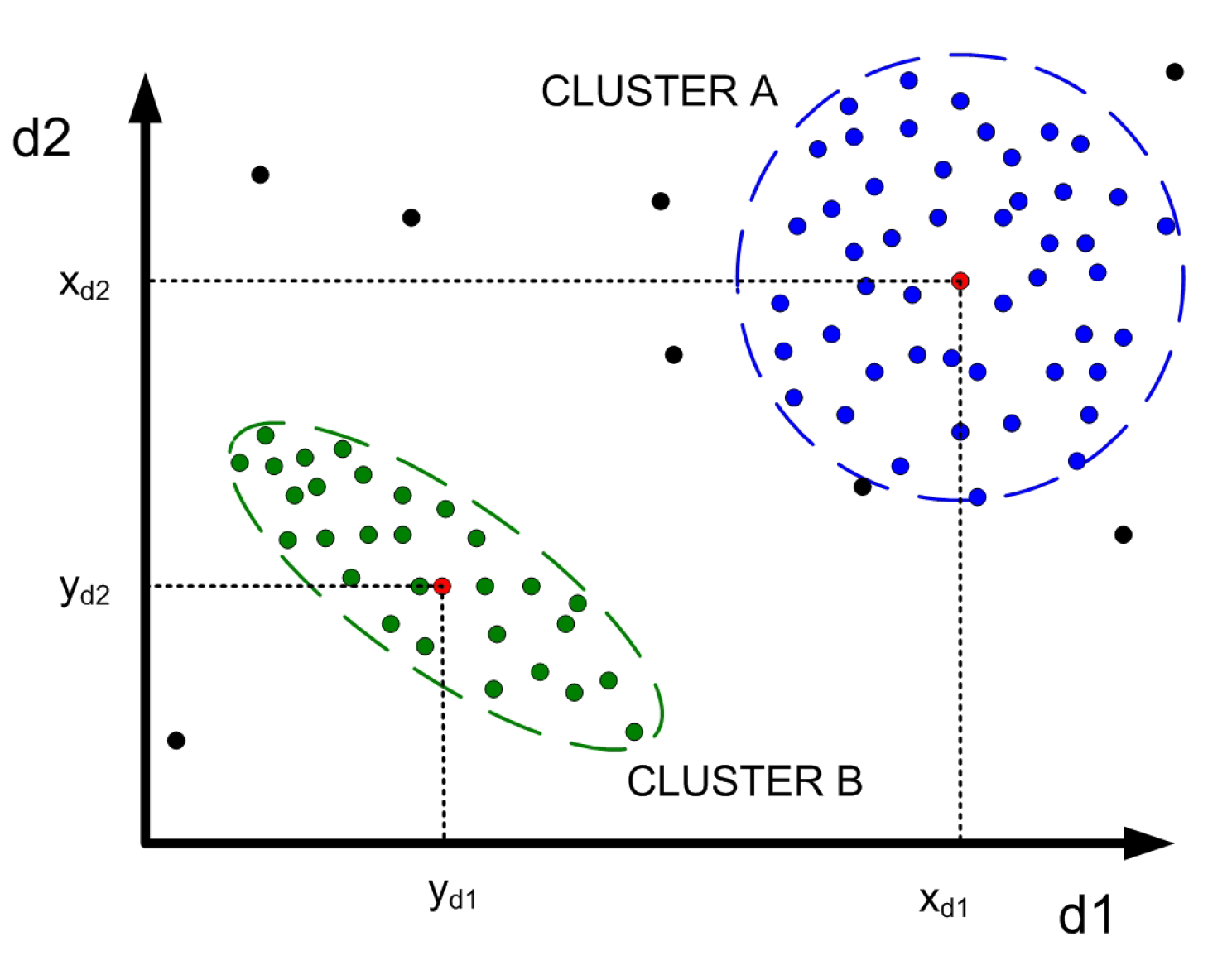
Table 1.
Notation.
| characteristic j of object i | |
| characteristic j of centroid k | |
| N | number of objects |
| c | numer of centroids |
| function distance among two objects, i and k | |
| d | number of characteristics (dimension) of the objects |
| fuzzy membership of the object i to the cluster k | |
| U | fuzzy membership matrix, with c rows and N columns |
| m | fuzziness index, higher than 1 (usually 2) |
| J | cost index to minimize |
| p | total number of samples or time instants |
| mean value (or vector of mean values per dimension) of a series x of objects or data |
Table 2.
Types of segmentation algorithms according to the dynamic nature of the data and classes.
| Type | Data | Classes | Segmentation Type |
|---|---|---|---|
| 1 | Static | Static | Static (classic) |
| 2 | Static | Dynamic | Dynamic. Centroids and classes are updated with each new cycle |
| 3 | Dynamic | Static | Dynamic. The centroids are represented by trajectories of their dimensions. Fixed number of classes |
| 4 | Dynamic | Dynamic | Dynamic. The centroids are represented by trajectories of their dimensions. The number of classes is updated with each new cycle |
Table 3.
Tested clustering algorithms for time series.
| No. | Base Clustering Technique | Dynamic Similarity Measure | Clustering Algorithm |
|---|---|---|---|
| 1 | K-means | Euclidean distance | END-KME |
| 2 | K-means | Correlation | END-KMC |
| 3 | K-means | Distance Hausdorff | END-KMH |
| 4 | K-means | Euclidean distance | K-means (modified) |
| 5 | FCM | Euclidean distance | END-FCME |
| 6 | FCM | Correlation | END-FCMC |
| 7 | FCM | Hausdorff Distance | END-FCMH |
| 8 | FCM | Fuzzy membership functions | FFCM |
Table 4.
DB index clustering test results (best performance in bold).
| Cycle | END-KME | END-KMC | END-KMH | K-Means | END-FCME | END-FCMC | END-FCMH | FFCM |
|---|---|---|---|---|---|---|---|---|
| 1 | 2.348 | 5.918 | 3.204 | NaN | 4.131 | NaN | 6.181 | 8.114 |
| 2 | 3.151 | 5.650 | 2.680 | 2.285 | 3.848 | NaN | 7.449 | 7.050 |
| 3 | 2.314 | 5.836 | 3.039 | 1.594 | 2.792 | NaN | 5.201 | NaN |
| 4 | 1.894 | 5.674 | 3.759 | NaN | 5.801 | NaN | 5.103 | NaN |
| 5 | 2.967 | 5.674 | 3.136 | 2.421 | 3.699 | NaN | 4.184 | NaN |
| 6 | 2.589 | 5.267 | 3.049 | NaN | 3.175 | NaN | 6.444 | 6.527 |
| 7 | 2.336 | 5.951 | 3.497 | 2.183 | 8.750 | NaN | 6.552 | NaN |
| 8 | 2.501 | 5.854 | 3.202 | NaN | 4.143 | NaN | 5.881 | NaN |
| 9 | 2.483 | 5.758 | 3.204 | 1.390 | 4.866 | NaN | 16.863 | 9.270 |
| 10 | 2.689 | 5.878 | 2.995 | NaN | 2.909 | NaN | 4.738 | NaN |
Publisher’s Note: MDPI stays neutral with regard to jurisdictional claims in published maps and institutional affiliations. |
© 2022 by the authors. Licensee MDPI, Basel, Switzerland. This article is an open access article distributed under the terms and conditions of the Creative Commons Attribution (CC BY) license (https://creativecommons.org/licenses/by/4.0/).
Share and Cite
MDPI and ACS Style
Benítez, I.; Díez, J.-L. Automated Detection of Electric Energy Consumption Load Profile Patterns. Energies 2022, 15, 2176. https://0-doi-org.brum.beds.ac.uk/10.3390/en15062176
AMA Style
Benítez I, Díez J-L. Automated Detection of Electric Energy Consumption Load Profile Patterns. Energies. 2022; 15(6):2176. https://0-doi-org.brum.beds.ac.uk/10.3390/en15062176
Chicago/Turabian StyleBenítez, Ignacio, and José-Luis Díez. 2022. "Automated Detection of Electric Energy Consumption Load Profile Patterns" Energies 15, no. 6: 2176. https://0-doi-org.brum.beds.ac.uk/10.3390/en15062176
Note that from the first issue of 2016, this journal uses article numbers instead of page numbers. See further details here.