1. Introduction
Most small-to-medium office buildings and residential buildings in India use ceiling fans and/or room air conditioners (RACs), such as split and variable-refrigerant-volume air conditioners to maintain thermal comfort (satisfaction) [
1,
2]. Such buildings are usually called mixed-mode buildings, where a distinct period for natural ventilation and air-conditioning exists. Often, simple occupant controls are used, such as opening and closing the windows and adjusting the AC (cooling) set point temperature and ceiling fan speed [
3,
4,
5]. The use of RACs results in significant energy consumption for space cooling and is expected to increase manifold in the coming decade due to factors such as the huge potential for RAC sales, increasing income levels and expectations of thermal comfort, and increasing outdoor temperatures [
1,
6,
7].
To reduce space cooling energy consumption in buildings, key policy instruments in India include energy codes for commercial buildings (Energy Conservation Building Code—ECBC) and residential buildings (ECO NIWAS SAMHITA), which specify minimum performance requirements for building envelope and technical systems [
8,
9]; minimum energy performance standards (MEPS) for RACs and ceiling fans, which are regulated by the mandatory and voluntary Bureau of Energy Efficiency (BEE) (energy) star labelling scheme, respectively [
10,
11]; the Super-Efficient Equipment Programme (SEEP), which aims to introduce and deploy super-efficient 35W ceiling fans against a market average of 70 W ceiling fans [
12,
13]; and Energy Efficiency Services Limited’s (EESL) EESL Super-Efficient Air-conditioner Program (ESEAP), which has sold over 1300 Super-Efficient 1.5 TR (approximately 5.3 kW) capacity air conditioners (ACs) that are at least 15% more efficient than the BEE’s five-star labelled ACs.
In addition to energy efficiency, appliance usage (i.e., user behaviour) plays a vital role in energy consumption [
14,
15,
16]. For example, behavioural aspects, such as AC (cooling) set point temperature and its operating duration, influence energy consumption [
17,
18]. In addition, simulation studies indicate that the simultaneous use of ACs with elevated air speed results in energy savings [
19] because similar levels of thermal comfort satisfaction can be felt at a higher AC set point temperature in the former case compared with the latter case. However, in Indian buildings, the effect of AC usage behaviour on space cooling energy consumption, and the effect of elevated air speed through the use of ceiling fans on indoor operative temperature (a critical parameter for determining thermal comfort) during AC usage are not widely studied, especially through field studies (see
Section 1.3).
To comprehend the objectives of the study, it is important to understand the methods used to define thermal comfort in mixed-mode buildings, how to enhance thermal comfort and achieve energy savings with elevated air speed, and key gaps in the current research. Therefore, in the following sub-sections of this introduction, thermal comfort models in mixed-mode buildings, the enhancement of thermal comfort and energy savings with elevated air speed, gaps in the current research, the objectives of the study and the structure of the paper are presented.
1.1. Thermal Comfort Satisfaction in Mixed-Mode Buildings
Thermal comfort satisfaction is crucial for the wellbeing and productivity of occupants. Establishing ‘thermal comfort for all’ through sustainable and smart space cooling technologies, aligned with the greenhouse gas reduction goals, is a priority for the Government of India [
20]. Thermal comfort in buildings is usually defined by using static models, such as Fanger’s predicted mean vote-predicted people dissatisfied (PMV-PPD) model, and variable models, such as the adaptive thermal comfort (ATC) model [
21,
22,
23]. Because of their wider acceptance, e.g., in international thermal comfort standards and national building energy codes and their fundamental differences, both the PMV-PPD model and an ATC model for India are considered in this study.
PMV is expressed in relation to the various thermal loads in the space by considering four environmental variables: air temperature (
), mean radiant temperature (
), air velocity (
), and relative humidity (
), as well as two occupant variables: clothing resistance (
clo) and the activity level of the occupants (
met). PMV is then expressed as an index that predicts the mean value of thermal sensation votes on a sensation scale between −3 and +3, which correspond to cold and hot, respectively. PPD is an index that estimates the percentage of thermally dissatisfied people and is expressed as a function of the PMV based on an empirical relation [
24].
The ATC model assumes that the occupants’ thermal comfort preferences are shaped by their past and present experiences in relation to the outdoor environmental conditions and behavioural adaptations. Furthermore, it assumes that thermal discomfort is mitigated through appropriate actions, such as opening the windows, adjusting ambient air velocity and AC set point temperature, and wearing appropriate clothing. Adaptive models are developed based on thermal comfort field surveys and are usually specific to climate, region, and building typology and operating mode (i.e., naturally ventilated, mixed-mode or air-conditioned). Indoor operative temperature,
, is a key parameter for expressing thermal comfort satisfaction using ATC models. It is defined as the weighted average of the air temperature and mean radiant temperature, and weighed by their respective heat transfer coefficients,
(see Equation (1)) [
25].
Usually,
is taken as 0.5 for practical purposes; however, technically, this is only valid when
. The ATC model expresses thermal comfort satisfaction in categories of acceptability bands around a neutral operative temperature,
.
is a function of the chosen outdoor environmental parameter, such as the mean monthly outdoor air temperature, which is given by the following [
26]:
where
is the indoor neutral operative temperature,
and
are constants that are specific to the ATC model and
is the chosen outdoor environmental parameter, which is usually valid for a limited range of
. Thermal comfort satisfaction is expressed in bands of acceptability between which 90, 85, and 80% of the occupants are satisfied. The bands are given by
, where
are the bands of acceptability between which 90, 85, and 80% of the occupants are satisfied, respectively. Thermal comfort conditions in the chosen acceptability band are met when
is within the range of
.
1.2. Elevated Air Speed for Enhancing Thermal Comfort in Mixed-Mode Buildings and Resulting Energy Savings
In warm and hot climates, air movement near the skin enhances the evaporation of sweat, reduces heat stress, and helps in maintaining thermal comfort. Studies conducted through the use of thermal mannequins [
27], human subjects [
27,
28,
29], and transient computational fluid dynamics [
30,
31,
32] consistently show that compared to a certain temperature that provides thermal comfort, similar levels of thermal comfort can be felt at higher temperatures with a corresponding increase in air velocity (i.e., due to elevated air speed).
Various empirical indices and normographs are used to assess the effects of elevated air speed on thermal comfort [
33,
34]. This study uses a widely accepted method, the Standard Effective Temperature (SET) method provided in the international standard, ASHRAE standard 55 Thermal Environmental Conditions for Human Occupancy. As per ASHRAE standard 55, if air velocity,
, is increased by
, the maximum operative temperature,
(
), in a comfort band, can be increased correspondingly, by
(cooling effect), to a new adjusted maximum operative temperature,
[
25]. However, as per ASHRAE standard 55, this is only applicable to enhance thermal comfort in buildings with natural ventilation. It further recommends limiting indoor air speed to 1.2 m/s when local control over airspeed is enabled. Without control, the limits for air speed are 0.8 m/s and 0.15 m/s for operative temperatures above 25.5 °C and below 22.5 °C, respectively [
25]. The latter limit is to avoid cold draughts [
35]. However, in warm climates, field studies indicate a clear preference for higher air speeds than the limits prescribed by ASHRAE standard 55 [
28,
36,
37], including in India [
5,
38,
39,
40,
41]. Studies indicate that air velocity limits may be appropriate for functional reasons, but they have a limited effect on thermal comfort conditions and behavioural adaptation [
28].
In mixed-mode buildings, the cooling effect (
) due to elevated air speed reduces space cooling energy by maximizing
, which enables extending the natural ventilation period, and increasing the cooling set point temperature (during air-conditioning period). This is often substantiated by building energy performance simulation studies [
42] and limited field studies exist [
43]. However, the application and benefits of the cooling effect due to elevated air speed through the use of ceiling fans in Indian mixed-mode buildings is unclear, especially through field studies.
1.3. Gaps in Current Research
In research on AC usage behaviour, detailed recordings of AC set point temperatures are not usually available [
44,
45,
46,
47]. Limited studies in India report AC and ceiling fan usage behaviour (e.g., preferences for AC set point temperature and fan speed) and its impact on energy consumption [
4,
48]. However, these are based on ‘right here and right now’ thermal comfort surveys and the behavioural parameters are not continuously monitored.
The effect of elevated air speed on thermal comfort is usually studied in controlled laboratory settings (typically in thermal comfort chambers) and via thermal comfort surveys. However, in the real world, the use of ceiling fans may increase indoor air temperature because convective surface heat transfer from the interiors (internal mass) and interior building surfaces increases with air velocity. The convective heat flux (exchange) (
) between a surface
and the air is given by the equation:
where
is the surface convective heat transfer coefficient between air and the surface
,
is the air temperature, and
is the surface temperature.
Peeters et al. analysed the effect of an unsteady flow on convection coefficient induced by various factors such as walking in the space, due to fans or the closing or opening of doors; obstructions within the zone such as furniture and window blinds; and internal gains. They observed that unsteady flow due to fan-induced air movement (air velocity in the range of 0.2 m/s to 1.2 m/s) leads to a considerable mixing of air in the space and resulted in a uniform space temperature, which only takes a short time (approx. 5 min) to stabilize [
49]. Choosing appropriate surface heat transfer coefficients is important for accurately calculating space cooing and heating loads while conducting dynamic building energy performance simulations [
50,
51]. In thermally insulated buildings and during air-conditioned periods, a sensitivity study shows that increasing the surface heat transfer coefficient from 8.3 Btu/h-ft2 (47.12 W/m
2K) to 12.0 Btu/h-ft2 (68.13 W/m
2K) (44% increase) changes cooling loads by less than 2%, which is negligible [
52]. However, most buildings in India do not have thermal insulation, which may lead to higher indoor surface temperature for external surfaces compared with building with thermal insulation. Moreover, building simulation studies that show energy savings due to elevated air speed often simply change the AC set point temperature with a corresponding increase in the air speed (e.g., by using the SET method). It is unclear whether the static or dynamic values for surface heat transfer coefficients assumed in such studies sufficiently represent the actual values. In addition, heat is dissipated from the motor of the ceiling fan (although, the motors are increasingly becoming efficient). These factors may result in an increase in the operative temperature and may reduce the benefits of the cooling effect due to elevated air speed. This phenomenon is not widely studied and is not clearly captured in thermal comfort chambers and surveys.
1.4. Objective of the Study
This paper analysed the impact of AC usage behaviour on energy consumption and the effect of elevated air speed, through the use of a ceiling fan, on operative temperature. This helps to increase the understanding on how to achieve an optimum AC set point temperature and air velocity, which would allow us to maintain thermal comfort while achieving energy conservation in mixed-mode buildings in India.
2. Methods and Materials
AC usage behaviour as a measure of thermal comfort and energy consumption and the effect of elevated air speed, through the use of ceiling fans, on indoor operative temperature are investigated through field studies. For monitoring and collecting key parameters, such as AC set point temperature (including on/off state), operative temperature and energy consumption, the study uses custom-built and low-cost micro-controller devices.
Three separate field studies were conducted. In the field study 1, AC usage behaviour was studied. In the other two field studies, 2a and 2b, the effect of elevated air speed through the use of ceiling fans on indoor operative temperature was studied.
The location and procedure of the field studies, instruments used in the study and their accuracy, and data collection and cleaning procedures are explained in the following sub-sections.
2.1. Location and Procedure of the Field Studies
All the three field studies were conducted in typical Indian residential bedrooms. The pictures have not been presented for privacy reasons. In general, the bedrooms contain items of furniture, such as furnished double beds, dressing tables, and wardrobes (either free standing or built into the wall). Further specifications of the rooms, such as dimensions and occupancy and their geographical location, can be found in the following sub-sections.
2.1.1. Field Study 1: AC Usage Behaviour
Field study 1 was conducted in the bedroom of a typical high-rise two-bedroom residential unit (2BHK) (middle floor) in the city of Ahmedabad, India, which has a hot-dry climate as per ECBC. The room was equipped with a remote-controlled wall-mounted split AC with a capacity of 1.5 TR (5.3 kW approximately) and a ceiling fan with a diameter of 1200 mm. The dimensions of the room are 3 m × 3.5 m × 3 m (height) and a window (single glazed and UPVC frame) of approximately 9 m
2 is located on one of the two external walls. Typically, the room is occupied during the nights (08:00 p.m.–06:00 a.m.) by two adults (30–40 years old) and one child (5-year-old) and intermittently occupied during the day on weekends or holidays. The volunteers of the study use the bedroom in mixed-mode operation. That is, they turn on the AC only when they feel that the thermal comfort conditions are not met, e.g., through natural ventilation. Windows are usually kept closed and the curtains are drawn over when the AC is turned on. The field study was conducted between 28 June 2021 and 8 August 2021. Key parameters that influence AC usage behaviour, i.e., air and globe temperature and relative humidity in the bedroom, were continuously recorded. Each time AC was used, the infrared (IR) signal from the remote control was recorded. A smart plug was used to measure the daily energy consumption of the AC (see
Section 2.2 for more details on instruments).
2.1.2. Field Study 2a: Effect of Elevated Air Speed through Ceiling Fan Operation on Indoor Operative Temperature
This is a pilot study to verify and explain, in principle, the phenomenon of ‘cooling effect reduction’. Field study 2a was conducted in a ground-floor bedroom of a three-storey residential building in the city of Hyderabad, India, which has a composite climate as per ECBC. The room was equipped with a remote-controlled wall-mounted split AC of 1.5 Ton (5.3 kW approximately) and a ceiling fan. The dimensions of the room are 3 m × 3.5 m × 3 m (height) and two windows (single glazed and wooden frame) of approximately 1.8 m2 are located on each of the two external walls. During the experiment, textile curtains were drawn over the window. The experiment was conducted for one day (on 30 April 2021), during the afternoon. The room was never occupied during the experiment. The ceiling fan was operated for approximately 4.5 h at each of the available four speed settings for half an hour, in descending and ascending orders of speed, with zero speed setting in between them. The AC set point temperature was set to 24 °C. Before beginning the experiment, the room was maintained at the AC set point temperature of 24 °C and fan speed setting of five for half an hour to one hour to achieve thermal stabilization. During the experiment, the air and globe temperatures and relative humidity were recorded.
2.1.3. Field Study 2b: Effect of Elevated Air Speed through Ceiling Fan Operation on Indoor Operative Temperature
This study is in continuation of field study 2a to analyse the principle of cooling effect reduction at various AC set point temperatures. Field study 2b was conducted in a top-floor bedroom of a three-storey residential building in the city of Hyderabad, India, which has a composite climate as per ECBC. The room was equipped with a remote-controlled wall-mounted split AC of 1.5 Ton (5.3 kW approximately) and a ceiling fan. The dimensions of the room are 4 m × 3.5 m and a window of approximately 4 m2 is located on one of the two external walls. The experiment was conducted for four days, mostly during the afternoon. During the experiment, textile curtains were drawn over the window. The room was intermittently occupied during the experiment by an adult (34 years old) and one child (eight years old). On all four days, the ceiling fan was operated for approximately 5.5 h at each of the available five speed settings for half an hour, in descending and ascending orders of speed, with zero speed setting in between them. The AC set point temperature was set to 24, 26 and 28 °C on days one, two and three, respectively. On day four, the room was naturally ventilated. Before beginning the experiment for the day, the room was maintained at the AC set point temperature of the day and fan speed setting five for half an hour to one hour to achieve thermal stabilization. During the experiment, the air and globe temperatures and relative humidity were recorded.
2.2. Instruments and Accuracy
For data collection, two modules were developed and used. One is a comfort module that records the air temperature, globe temperature and relative humidity, and the second is an IR module that records the AC IR signals (
Figure 1). The comfort module was carefully placed to avoid any proximate heat sources or heat sinks. Both modules use suitable sensors that are connected to Arduino-based Wi-Fi microcontroller boards with 4MB flash based on ESP-8266EX microchip and are powered by a micro-USB cable. For measuring globe temperature, a DS18B20 temperature sensor was inserted into a 40 mm diameter ping-pong ball and was sealed so it was air-tight. At lower airspeeds and radiant loads (such as in this study), such a small globe thermometer can provide reliable results [
53,
54,
55]. The data were recorded at specified intervals on an on-board micro-SD card and additionally sent to a remote MySQL database [
56]. A smart plug was placed between the AC power plug and mains socket to record the AC energy consumption.
Table 1 shows the details of various sensors and components used in the modules.
Prior to the field studies, a prototype of the comfort module was assembled and tested for its accuracy. However, the prototype used an SHT31 sensor, which is technically similar to the SHT30 sensor that was used in the comfort module in the study. For assessing its accuracy, the readings from the prototype were compared with a reference instrument, an accurate ALMEMO board in a rapid assessment approach. The measurements from the prototype and ALMEMO were taken by placing them side-by-side for approximately three hours in a centrally heated open hall (
Figure 2). For brief durations, a variety of ambient temperature and humidity and air velocity (AV) conditions were maintained by opening and shutting the external shutters of the hall, and by using a pedestal fan (see
Table 2). Self-heating in the sensors, and localized heating due to the heat emitted by the micro-controller located at the base of the prototype may affect the accuracy of the measurements from the sensors, which are approximately 10 cm above the base. To study the influence of self-heating, the prototype base was covered with aluminium foil during the first half and the foil was removed during the second half of the procedure. In addition, infrared images of the equipment were taken at different intervals.
Although all comfort modules that are used in the field studies were not tested in this manner, the results from prototype testing showed they can be reliably used. Especially, the changes in the air and globe temperatures and relative humidity were measured at sufficient resolution to reliably study the difference (delta) in values and patterns. Furthermore, uncertainty analysis was carried out to analyse the results by considering errors in measurements, where analyses with absolute values are necessary (e.g., in thermal comfort PMV-PPD and ATC). The results of the testing are presented in
Appendix A. Programming language R [
63] was used to analyse the results of testing and plotting was carried out by using R package ggplot2 [
64].
2.3. Data Collection and Cleaning
In the comfort module, air temperature and relative humidity were recorded at two-second intervals, and the globe temperature was recorded at an interval of 10 s on the on-board micro-SD card. In addition, all these parameters were sent to the remote MySQL database by using the HTTP protocol via Wi-Fi in 10-minute intervals. The IR module recorded the AC IR signals on the on-board micro-SD card and transmitted it to the MySQL database whenever a signal was received. Outdoor weather data were taken from OpenWeatherMap [
65].
For field study 1, data from the MySQL database were used and for field study 2, data from the on-board micro-SD card were used. An insignificant number of corrupt entries of the date–time format were found and removed from the data on comfort modules. Data from the IR remote required extensive parsing, visual inspection, and cleaning. Discrepancies in the data primarily include duplicate, stray and missing signals. Data of interest from the IR module include the timestamp of the signal, AC set point temperature including on and off signals, and AC fan speed. Signals for each day were plotted with temperature and humidity data and visually inspected for their accuracy and were slightly adjusted, if necessary, to correctly reflect the temperature and humidity profile. For field study 1, data from 17 days with complete and accurate data from both comfort and IR modules were considered for the study. Data from smart plug were collected via a smartphone app. Although the app shows instantaneous values of power voltage, current and power consumption, these values could not be recorded. Only daily energy consumption was recorded. Primarily, programming language Python [
66] was used for data analysis and plotting, including the packages Pandas [
67], SciPy [
68] and statsmodels [
69] for data analysis, and packages Matplotlib [
70] and Seaborn [
71] for plotting.
3. Results
3.1. Field Study 1: AC Usage Behaviour
In the following sub-sections, AC on/off behaviour is studied by analysing three features. The first feature considers air temperature and relative humidity, as these can be easily measured, and can be used for controlling the AC. The second and third features are based on two thermal comfort standards, which consider more parameters than air temperature and relative humidity. Thermal comfort satisfaction was analysed by using a static temperature model, i.e., Fanger’s PMV-PPD model, and an adaptive model, i.e., Indian Model for Adaptive Comfort (IMAC).
3.1.1. Air Temperature and Relative Humidity
Figure 3 (left) shows the instantaneous values of air temperature and relative humidity when turning the AC on and off. Because the distributions of air temperature and relative humidity are not normal, and assuming that both these parameters are paired, a Wilcoxon Signed-Rank test was performed to assess whether these values are distinct when turning the AC on and off. The p-values for air temperature and humidity for turning the AC on and off are 4 × 10
−9 and 0.00149, respectively, indicating that the values are from different distributions and are distinct.
Figure 3 (right) shows the (periodic) time-weighted average of air temperature and relative humidity for each period, i.e., the period between whenever the AC set point temperature changed. The usual preference for AC set point temperature is between 25 and 29. The mean and median values of air temperature and relative humidity that result in turning the air conditioner on and off are shown in
Table 3. The difference between the mean/median air temperatures and relative humidity values that result in turning the air conditioner on and off are 1.95/2.14 K and 5.62/4.92%, respectively.
Figure 4 shows the drop in air temperature and relative humidity for each cycle, i.e., cycle between whenever the AC is turned on and off (on/off cycle), and the duration of the cycle. The mean/median values for drop in air temperature and relative humidity for on/off cycle are −2.09/−1.95 K and −5.63/4.77%, respectively. The mean/median values for the duration of the on/off cycle are 2.95/1.9 h. The drop in air temperature increases with the running time of the air conditioner up to approximately four hours of continuous running time. However, the continuous running time (duration) of the on/off cycle does not necessarily result in a corresponding and proportionate decrease in the room air temperature and relative humidity. Beyond six hours of continuous running time of the air conditioner, the drop in air temperature does not significantly increase with running time, although a certain drop is maintained as per the AC set point temperature. This is expected as the rate of change of air temperature is high initially when the AC is turned on or set point temperature is changed, and later, the air temperature is maintained accordingly.
3.1.2. Thermal Comfort: PMV-PPD
For calculating PMV-PPD, environmental variables—air temperature and relative humidity—were measured and mean radiant temperature was calculated using the measurements of globe temperature; air velocity was assumed to be approximately 0.2 m/s based on the occupant reported regulator speed of the ceiling fan, which is one; occupant variables—clo and met values—were taken as 0.96 and 0.7, respectively, which are suitable for sleeping activity. PMV-PPD indices were calculated using the Python package pythermalcomfort, as per the ASHRAE standard 55 [
72].
Figure 5 shows the relationship between the PMV and PPD indices corresponding to turning the AC on and off. The graph on the top right shows the PMV-PPD values based on field measurements. Because the comfort module was not calibrated, an uncertainty analysis was conducted to build confidence in the results obtained from recorded measurements. For this purpose, an error band was assigned for all the variables based on the results of prototype testing and the literature (see
Table 4) and the resultant PMV-PDD values corresponding to turning the AC on and off were plotted as boxplots adjacent to the results from measurements. For the uncertainty analysis, 14,336 samples were generated and analysed using the Python package SALib [
73]. Furthermore, a
z-test test was performed to assess whether the values of PMV and PPD are distinct for turning the AC on and off. The
p-values of the
z-test for both PMV and PPD are almost equal to zero, indicating that the values are from different distributions and are distinct.
The PMV-PPD results from both measured and uncertainty analyses show that most instances (i.e., interquartile range between 25 and 75 percentiles) of turning on the AC can be found between sensation votes one and two and most instances of turning off the AC can be found between sensation votes zero and one (
Figure 5). Similarly, the AC is mostly turned on when the PPD is above 30%. This indicates that up to 70% of the occupants are satisfied with the thermal comfort conditions between PMV of zero and one and that they do not require AC usage at these conditions.
Figure 6 shows the probability of the AC being turned on and off at various values of PPD from uncertainty analysis binned in 5% values. The probability of the AC being turned off is very high when the PPD is between 5and 10% and it reduces considerably in the next two bins of PPD between 10–15% and 15–20%, although the probability of the AC being turned on is still higher than the AC being turned off in those bins. Between a PPD of 30 and 40%, the probability of the AC being turned on was almost equal to that of the AC being turned off, and beyond a PPD of 40%, the probability of the AC being turned on increased compared with that of the AC being turned off.
3.1.3. Thermal Comfort: ATC Model Using Indian Model for Adaptive Comfort (IMAC)
For analysing thermal comfort as per ATC, this study used IMAC for mixed-mode office buildings, due to the lack of an alternative and authoritative adaptive model for thermal comfort in Indian residential buildings [
27]. IMAC is expressed as a function of neutral operative temperature (thermal neutrality) and 30-day outdoor mean air temperature (see
in Equation (2)). IMAC proposes temperature acceptability bands for 80%, 85% and 90% when the occupants are satisfied.
Figure 7 shows the relation between thermal comfort as per IMAC for mixed-mode buildings and turning the AC on and off. The graph shows the recorded measurements as points. Because the comfort module used in the study was not calibrated, an uncertainty analysis was conducted to build confidence in the results obtained from recorded measurements. For this purpose, an error band was assigned for all the variables (see
Table 5) and the resultant values of indoor operative temperature corresponding to turning the AC on and off were plotted as boxplots adjacent to the results from measurements. For the uncertainty analysis, a total of 8192 samples were generated using the Python package SALib.
The results from measurements and uncertainty analysis show that most instances of turning on the AC are near to and beyond the upper bound of 85% acceptable limit band, while the AC was mostly turned off between the neutral operative temperature and upper bound of 90% acceptable limit band (
Figure 7). Furthermore, a
z-test test was performed to assess whether the values of indoor operative temperature are distinct for turning the AC on and off. The
p-value of the
z-test is almost equal to zero, indicating that the values are from different distributions and are distinct.
Figure 8 shows the probability of the AC being turned on and off within various bands of thermal comfort as per IMAC model. The probability of the AC being turned off is very high within the bounds of 90% limit band. Beyond the upper bound of 85% limit band, the instances of AC turned on increase significantly.
3.1.4. Energy Consumption of the Air Conditioner
The measurements obtained from the field study that influence energy consumption of the air conditioner include: indoor relative humidity; AC set point temperature; outdoor relative humidity; difference between indoor and outdoor temperatures; difference between indoor and outdoor relative humidity; outdoor temperature; drop in indoor relative humidity during each period of change in AC set point temperature; difference between indoor air temperature and AC set point temperature; drop in indoor air temperature during each period of change in AC set point temperature; drop in indoor globe temperature during each period of change in AC set point temperature; indoor globe temperature; indoor air temperature; and the total running time of the air conditioner.
As the energy consumption values are only available as daily values, the time-weighted averages were considered for all the parameters, except for the total running time of the air conditioner.
Energy consumption with respect to the most influential parameters shows that the data are not always normally distributed and is possibly non-linear and non-monotonic. However, it has a monotonic relationship with the total running time of the air conditioner. Therefore, a linear and second-order polynomial regression was conducted between energy consumption and total running time and other parameters. This was conducted for a dataset of total 17 days, and another dataset of 11 days without the outliers. Energy consumption (in kWh) showed a significant linear relationship with the total running time (in hours) and AC set point temperature (typically, in °C or simply set point number). The standardized regression coefficients (SRC) for these influential parameters are shown in
Table 6. There is almost no difference in SRC between data with and without outliers. The
p-values for both data are <0.05. However, the R-squared, and adjusted R-squared values are 0.845 and 0.806, and 0.649 and 0.651 for data with and without outliers, respectively, which implies the difference in the predictive capability of the model with and without outliers, respectively.
Figure 9 shows the relationship between the two influential parameters on a scatterplot for all values of daily energy consumption (including the outliers). The energy consumption increases with total running time and decreases with AC set point temperature. A residual analysis was conducted to further determine the significance of the results from linear regression, which are provided in
Appendix B.
3.2. Field Study 2a: Effect of Elevated Air Speed through the Use of Ceiling Fans on Indoor Operative Temperature
Figure 10 shows the indoor operative temperature at AC set point temperature 24 °C at various fan speeds and the mean operative temperature for each fan speed. Compared with the operative temperature at fan speed one, the operative temperature increased by up to a maximum of 2.33 °C at fan speed four.
The cooling effect (
) and rise in operative temperature because of elevated air speed at various fan speeds compared to the operative temperature at fans speed two are shown in
Figure 11 (left). The cooling effect from elevated air speed was derived theoretically using the SET method. The fan speeds were not measured and are assumed conservatively (on the higher side) at the height of a working plane (900–1200 mm) based on the values in the literature [
27,
74,
75,
76]. When the fan speed was increased from one to two, the cooling effect predicted that the operative temperature can be increased by 1.09 °C to 1.75 °C to retain a similar thermal sensation that can be felt at the operative temperature at fan speed one. However, an increase in the fan speed from one to two increased the operative temperature and thereby reduced the predicted benefit of the cooling effect by 1.2 °C. Although the cooling effect reduction was higher when the fan speed increases from one to five than it decreases from five to one, cumulatively, the effect is still substantial as at least 60% of the benefits of the cooling effect are reduced due to rise in operative temperature (see
Figure 11 (right)).
3.3. Field Study 2b: Effect of Elevated Air Speed through the Use of Ceiling Fan Operation on Indoor Operative Temperature
Figure 12 shows the indoor operative temperature and its mean at AC set point temperatures of 24 °C, 26 °C, and 28 °C and during natural ventilation and at various fan speeds (FS). In addition, the acceptable increase in operative temperature as predicted by the cooling effect at various air speeds as compared to the operative temperature at fan speed zero is shown. At all AC set point temperatures, the operative temperature increases with fan speed, although, the increase in operative temperature is higher at lower AC set point temperature. During natural ventilation, an increase in fan speed had a insignificant effect on operative temperature. Our analysis showed that intermittent occupancy did not have any significant impact on indoor operative temperature.
Figure 13 shows the percentage of cooling effect reduction due to the rise in operative temperature during the second experiment. In general, the cooling effect reduction decreases with fan speed and AC set point temperature. For all AC set point temperatures, the cooling reduction effect is significant when the fan speed increases from zero to one and from one to two, i.e., from seemingly still conditions to slight air movement compared with the increase in subsequent fan speed steps.
4. Discussion
4.1. AC Usage Behaviour and Thermal Comfort Satisfaction
It appears that turning the AC on and off is significantly driven by air temperature and relative humidity. However, while both air temperature and relative humidity are significant parameters for turning on the AC, only air temperature appears to be a significant parameter for turning off the AC (see
Figure 3 and
Figure 4). Furthermore, the AC usage behaviour in the field study suggests a clear need for the use of AC to achieve thermal comfort satisfaction and can be considered as energy-conscious behaviour. While the PMV-PPD model predicts that the probability of the AC being turned on and off within the bounds of 90% people being satisfied is approximately 12% and 55%, respectively (see
Figure 6, cumulative value of probability of PPD bins five and 10), the IMAC model predicts these values to be 20% and 89%, respectively (see
Figure 8, cumulative value of probability of upper 85%–upper 90% and upper 90%–lower 90%). Although, the AC usage behaviour correlates with the PMV-PPD thermal comfort model, the PPD value is as high as 30% when the AC is turned off (usually, <20% is considered desirable). Considering that the AC is turned on when there was thermal discomfort and turned off when the thermal comfort satisfaction was met, the thermal comfort predictability of the IMAC model is higher than the PMV-PPD model.
4.2. AC Usage Behaviour and Energy Consumption
As the total running time of AC increases the energy consumption, the results were further analysed to find the parameters that influence the total running time of AC, such as indoor and outdoor temperatures. However, there were no clear patterns or significant correlations found. Reasonably, a key aspect that determines the total running time is turning off the AC, which has a strong correlation with indoor air temperature. The drop in air temperature, for each cycle of turning the AC on and off, increases with the running time (at least up to first four hours; see
Figure 4) and consequently, the running time increases the AC energy consumption.
Figure 14 shows the empirical cumulative distributive function of drop in air temperature between each on and off cycle. The probability of drop in air temperature of at least −3 °C is 79%, and the percentage of hours the air conditioner runs to achieve a temperature drop of at least −3 °C is 67.5%. This indicates that there is a 79% probability that comfort conditions can be maintained by achieving a temperature drop of 3K. If this drop can be achieved, as much as possible, through passive measures (e.g., improved shading, thermal insulation, etc.), the running time of the air conditioner can be reduced by 67.5%, and consequently at least 58.4% of AC energy can be saved at a constant set point temperature based on the SRC value of 0.8655 for the relation between running time and energy consumption (see
Table 6). Similarly, even a 1K drop in temperature could reduce the running time by 32.2% and energy consumption by at least 27.8%. As the occupants have a clear preference for air speed during the operation of the air conditioner, additional energy savings due to elevated air speeds are not possible. Similarly, there is a 70% probability that comfort conditions can be maintained by achieving a relative humidity drop of 15% with a running time of 70.9%. However, as a drop in air temperature is more significant than relative humidity for turning off the air conditioner, reducing relative humidity may not significantly impact the AC running duration.
4.3. Optimum AC Set Point Temperature and Air Velocity for Energy Conservation While Maintaining Thermal Comfort
In
Figure 10, from field study 2a, a similar thermal comfort sensation can be felt at an operative temperature of 24.6 °C and at fan speed one, and at an operative temperature of 27 °C and at fan speed two (due to cooling effect). Although ceiling fan energy consumption increases with its speed, the net energy consumption of both the AC and ceiling fan is, presumably, lesser in the latter conditions, because, typically, cooling energy saving due to increase in the AC set point by approximately 2 °C, to achieve an operative temperature of 27 °C, is higher than the additional energy consumption of the ceiling fan by increasing its speed by one step (to fan speed two). Although it appears that elevated air speed results in energy savings, despite the cooling effect reduction, further questions arise:
Is the operative temperature of 27 °C maintained at an AC set point temperature of 27 °C and fan speed 2?
What would be the profile of the cooling effect and cooling effect reduction at various AC set point temperatures and air speeds?
What would be, and how do we choose, an optimum combination of AC set point temperature and fan speed to optimize energy savings due to elevated air speeds?
These questions can be answered with the results of field study 2b, which was conducted to observe the effects of elevated air speeds on indoor operative temperature at three different AC set point temperatures, 24 °C, 26 °C, and 28 °C, and in addition, during natural ventilation (see
Figure 12). The band at operative temperature 26 ± 0.5 °C (band 1) can be taken as an example, say, as the desired temperature band that can be achieved because of elevated air speed relative to the operative temperature at AC set point temperature of 24 °C and fan speed zero. Theoretically, at an AC set point temperature of 24 °C and fan speed zero, the operative temperature in the range in band 1 can be achieved by increasing the fan speed to three or four. Logically, as a consequence, the AC set point temperature can be increased to 26 °C and fan speed to three or four to maintain the conditions in band 1. In agreement with this, the results show that band 1 can be achieved at AC set point temperature to 26 °C and at fan speeds to 2, 3 and 4. However, band 1 can also be achieved more energy efficiently at an AC set point temperature of 28 °C and at fan speeds 0, 1, 2, and possibly 3. Moreover, when the operative temperature is within the desired temperature band, it is efficient to maintain the fan speed at zero or at lowest possible fan speed, if a certain air speed is desired. Similarly, to maintain a desired temperature band of 28 ± 0.5 °C, say band 2, from a base AC set point temperature of 26 °C, theoretically, the AC set point temperature and fan speed can be at 28 °C and five. However, practically, there is a clear opportunity to increase the AC set point temperature beyond 28 °C, which will be more energy efficient.
In general, in air-conditioned environment, beyond 26 °C, thermal comfort satisfaction is a complex phenomenon influenced by a combination of air temperature, relative humidity and air velocity [
27,
28,
31], although the acceptance of a high temperature may be higher at high air speeds [
77]. Alternatively, as seen from field study 1, occupants may have a preferred air speed setting while using the air conditioner, which is mostly one in this case. In addition, beyond an operative temperature of 30 °C, thermal comfort studies in naturally ventilated buildings indicate that preference for air speed usually plateaus at about 0.6 m/s [
40] or a preference for air velocity of up to 1 m/s was noticed [
78]. Furthermore, this allowable increase in AC set point temperature is, however, case specific, and depends on multiple factors that affect heat load in the space. In addition, when there is a high cooling effect reduction, increasing the fan speed with or without increasing the AC set point temperature can be counterproductive.
In mixed-mode buildings, the expectation of energy savings and thermal comfort satisfaction due to elevated air speed through the use of ceiling fans could be case specific and could present an unfulfilled potential if a SET model is used to determine the allowable increase in operative temperature for a corresponding increase in air velocity. Therefore, in mixed-mode buildings, during air-conditioned periods, it is recommended to set the AC set point to maintain the desired temperature band and set the ceiling fan to the minimum speed setting, at least until the operative temperature of 28 °C is reached. This is especially true for buildings that are prone to having high internal surface temperatures, e.g., in buildings without thermal insulation.
4.4. Limitations of the Study and Perspectives for Future Work
A key limitation of the study is the limited number of field studies. In field studies 2a and 2b, the actual energy consumption of the AC and fan at various AC set point temperatures and fan speed settings was not measured. In addition, the actual indoor air velocity was not measured in all field studies. However, this study is supported by reasonable assumptions, sufficient statistical analyses and discussion to illustrate the often overlooked and less studied aspects of AC usage behaviour and elevated air speed for thermal comfort. Moreover, the cheap cost of setting up the experiment and expanding its scope to include other observations, such as collecting energy consumption data in better time resolution, e.g., through the use of cost-effective energy metering modules [
79] and measuring supply and condenser air temperature of the air conditioner, can provide further significant insights into real-world AC energy consumption. The results of this study could be applicable to office buildings of similar size and construction.
Although the thermal comfort models show strong correlation with turning the AC on and off, they usually require precise measurements of air and globe temperatures and air velocity. However, challenges in taking accurate measurements can be overcome, for example, through machine learning techniques that are able to learn patterns for control, instead of relying on accurate measurements. Such data could be used to train machine learning models that can automatically control the air conditioner to maximize comfort and reduce energy consumption. They can further help in the predictive maintenance of ACs by using automatic fault detection and diagnostics management. For example, as bedroom AC is typically operated during night-time, and for longer durations, users may not be inclined to turn off the AC until they feel cold. Although most modern ACs are equipped with a timer function to automatically turn on/off the AC, the on/off function could be linked to influential parameters such as indoor air temperature and relative humidity to enhance thermal comfort and reduce energy wastage. Moreover, users can be provided with real-time feedback on energy consumption that motivates them to use AC judiciously and at high set point temperature. For example, in the present study, the automatic control of the AC can be accomplished by the addition of an IR LED to the IR module and providing it with a control logic [
80]. Furthermore, such devices can be easily integrated into homes, thus making them smart homes, and help smart grids to improve demand-side management, such as the Dispatchable Air-Conditioning Pilot Project (DAC) project in Auroville, India [
81,
82].
5. Conclusions
This study shows the significance of two critical parameters that influence the energy consumption of air conditioners, i.e., the AC set point temperature and running time, which is substantiated by a field study. In the current study, an indoor air temperature drop of 1–3 K, if achieved by passive means, resulted in significant energy savings with regard to space cooling. This range of temperature decreases is easy to achieve through passive means, such as improved shading, adding thermal insulation, improving the solar reflective index of walls and roof, and through optimum ventilation (e.g., night-time ventilation). Furthermore, we attempted to identify the phenomenon of cooling effect reduction due to the use of ceiling fans in mixed-mode buildings. The results indicate that it is energy efficient to use ACs at a high set point temperature and use ceiling fans at the lowest possible speed setting, especially at indoor operative temperatures of less than 28 °C, approximately. Although this study identifies the existence and potential for ‘cooling effect reduction’, further studies are required to reliably confirm this phenomenon. Especially, cooling effect reduction should be looked at holistically by considering its impact on space cooling energy consumption and thermal comfort satisfaction in various building typologies and construction types, e.g., in residential and office buildings; building with and without thermal insulation; and buildings with varying number of external surfaces.
Author Contributions
Conceptualization, methodology, formal analysis, investigation, visualization, and writing—original draft preparation, S.G.; writing—review and editing, methodology, and supervision—C.v.T. and R.R. All authors have read and agreed to the published version of the manuscript.
Funding
This project received a grant for purchase of the instruments and travel expenses from The Friends of the Wuppertal Institute (Die Vereinigung der Freunde des Wuppertal Instituts), a non-profit association. We acknowledge financial support from Wuppertal Institut für Klima, Umwelt, Energie gGmbH within the funding programme Open Access Publishing.
Institutional Review Board Statement
Not applicable.
Informed Consent Statement
Informed consent was obtained from all subjects involved in the study.
Acknowledgments
We are grateful to the volunteers Ankit Kumar, for participation in field study 1, and Budampati V S Sowmya and Gabbita Lakshmi Alankrutha, for conducting field study 2b. Many thanks also go to Stefan Thomas from Wuppertal Institute for his advice and feedback on the experiment and manuscript and supporting the research and grant application. Thanks are also due to Marc Syndicus and Rainer Ehrt from E3D—Institute of Energy Efficiency and Sustainable Building, RWTH University, Aachen, for their support in the testing of the prototype. We also thank Rainer Ehrt, especially for taking the time to share detailed and valuable information on electronics and other suggestions that helped in developing the modules, as well as Peri Kalyan Ram for discussions on the analysis of the results.
Conflicts of Interest
The authors declare no conflict of interest.
Nomenclature
| Item | Description | Unit |
| Clo | Clothing thermal insulation | clo |
| Internal Surface heat transfer coefficient | W/m2K |
| Met | Metabolic rate (metabolic equivalent of task) | met |
| Convective heat flux | W |
| Relative humidity | % |
| Air temperature | °C |
| Mean radiant temperature | °C |
| Operative temperature | °C |
| Maximum operative temperature | °C |
| Adjusted maximum operative temperature | °C |
| Neutral temperature | °C |
| Surface temperature | °C |
| Increase in operative temperature | °C |
| Air velocity | m/s |
| Adjusted (heat transfer) coefficient | - |
| Thermal comfort bands of acceptability for adaptive thermal comfort models | °C |
Appendix A. Results of the Rapid Assessment Testing of the Comfort Module Prototype
For assessment, the readings from the comfort module prototype were compared with an accurate reference instrument, ALMEMO. The measurements from the prototype and ALMEMO were taken by placing them side by side for approximately three hours in a centrally heated open hall (
Figure 2). For brief durations, a variety of ambient temperature and humidity, and air velocity (AV) conditions were maintained by opening and shutting the external shutters of the hall, and by using a pedestal fan.
Table 2 describes the ambient conditions maintained during the comparison procedure. The following sub-sections discuss the results of the testing process for ait temperature, relative humidity, globe temperature and infrared thermography.
Appendix A.1. Air Temperature
The graph and boxplot below show the measurements of air temperature and difference in air temperature between both devices, respectively (
Figure A1 and
Figure A2). During the steady-state conditions, when the rate of change of temperature is less than 0.2 K/min, the mean difference between air temperature measurements from both devices is 0.09 K. The difference increases during dynamic conditions (0.2–0.6 K/min) caused by the opening and closing of the external shutters, with mean and maximum differences of 0.2 K and 0.37 K, respectively. The difference is also lower when the aluminium foil covers the base, and when the air velocity is higher. During the entire period of the testing procedure, the mean difference was 0.07 K, and the error (difference) between the measurements was systematic, suggesting that the measurements of the prototype are reliable.
Figure A1.
Air temperature recorded by the Arduino prototype and Almemo instrument during various ambient conditions.
Figure A1.
Air temperature recorded by the Arduino prototype and Almemo instrument during various ambient conditions.
Figure A2.
Difference in air temperature recorded by the Arduino prototype and Almemo instrument during various ambient conditions.
Figure A2.
Difference in air temperature recorded by the Arduino prototype and Almemo instrument during various ambient conditions.
Appendix A.2. Relative Humidity
The graph and boxplot below show the measurement of relative humidity and difference in relative humidity between both devices, respectively (
Figure A3 and
Figure A4). The difference in relative humidity measurement by both devices increased during the dynamic period when the external shutters were opened and closed. However, the mean relative humidity values during the dynamic and steady-state conditions are close to each other, at 4.14 and 4.11, respectively, and the error (difference) is systematic. The aluminium foil at the base of the prototype and the change in air velocity did not have an impact on the measurements of relative humidity.
Figure A3.
Relative humidity recorded by the Arduino prototype and Almemo instrument during various ambient conditions.
Figure A3.
Relative humidity recorded by the Arduino prototype and Almemo instrument during various ambient conditions.
Figure A4.
Difference in relative humidity recorded by the Arduino prototype and Almemo instrument during various ambient conditions.
Figure A4.
Difference in relative humidity recorded by the Arduino prototype and Almemo instrument during various ambient conditions.
Appendix A.3. Globe Temperature/Mean Radiant Temperature (MRT)
The graph and boxplot below show the measurement of globe temperature and difference in globe temperature between both devices, respectively (
Figure A5 and
Figure A6). MRT was calculated using the globe temperature in accordance with ISO 7726:1998 using the python package pythermalcomfort. The difference in the measurement of globe temperature is almost twice that of the MRT. Similar to air temperature, the difference in measurements between both devices increases during dynamic periods. As the rate of change of MRT increased from 0.01 K/min to 0.3 K/min, the difference increased from approximately 0.5 K to 1.4 K. Although insignificant, this difference was lower when the aluminium foil was removed from the base and when the air velocity was increased. During the entire measurement period, and during the dynamic periods, the mean MRT differences were very close to each other, at 0.58 K, and 0.55 K., respectively, and the error (difference) between the measurements was systematic, suggesting that the measurements from the prototype are reliable.
Figure A5.
Air (ta), globe (tg) and mean radiant temperature (mrt) recorded by the Arduino prototype and Almemo instrument during various ambient conditions.
Figure A5.
Air (ta), globe (tg) and mean radiant temperature (mrt) recorded by the Arduino prototype and Almemo instrument during various ambient conditions.
Figure A6.
Difference in globe (tg) and mean radiant temperature (mrt) recorded by the Arduino prototype and Almemo instrument during various ambient conditions.
Figure A6.
Difference in globe (tg) and mean radiant temperature (mrt) recorded by the Arduino prototype and Almemo instrument during various ambient conditions.
Appendix A.4. Infrared Thermography
Infrared images show the surface temperatures of both devices (
Figure A7). Overall, the images show that the influence of localized heating due to the heat emitted from the micro-controller is negligible when the base of the prototype is covered with aluminium foil and when it is removed. For example, during the ambient condition ‘external gate opened’ and when the base was covered, the difference between the surface temperatures of globes of both instruments was 0.7 K. When the cover was removed and the surrounding air velocity was increased, the board appeared to have considerably cooled down, almost to the level of surface temperatures of the spheres. The difference in the surface temperatures of the spheres is 0.2 K.
Figure A7.
Infrared images of both devices during ambient condition ‘external gate opened’ (left) and ‘fan on’ (right).
Figure A7.
Infrared images of both devices during ambient condition ‘external gate opened’ (left) and ‘fan on’ (right).
Appendix B. Residual Analysis of Linear Relationship between AC Energy Consumption and Total Running Time of the Air Conditioner and Periodic Average of AC Set Point Temperature
A residual analysis was conducted to further determine the significance of the linear relationship between AC energy consumption and the total running time of the air conditioner and periodic average of the AC set point temperature (see section Energy consumption of the air conditioner) (
Figure A8). The residuals from the linear regression show a normal distribution (a), and the residuals are randomly distributed around zero against the fitted values (b). This suggests that the linear model satisfactorily explains the relationship.
Figure A8.
Residual analysis of linear relationship between AC energy consumption and total running time of the air conditioner and periodic average of AC set point temperature: (a) residuals showing normal distribution; (b) residuals randomly distributed around zero against the fitted values.
Figure A8.
Residual analysis of linear relationship between AC energy consumption and total running time of the air conditioner and periodic average of AC set point temperature: (a) residuals showing normal distribution; (b) residuals randomly distributed around zero against the fitted values.
References
- Kumar, S.; Kachhawa, A.; Goenka, A.; Kasamsetty, S.; George, G. Demand Analysis for Cooling by Sector in India in 2027; Alliance for an Energy Efficient Economy (AEEE): New Delhi, India, 2018; Available online: http://www.aeee.in/wp-content/uploads/2018/10/Demand-Analysis-for-Cooling-by-Sector-in-India-in-20271.pdf (accessed on 7 February 2022).
- Bhatnagar, M.; Mathur, J.; Garg, V. Development of reference building models for India. J. Build. Eng. 2019, 21, 267–277. [Google Scholar] [CrossRef]
- Honnekeri, A.N. Indoor Environmental Quality, Adaptive Action and Thermal Comfort in Naturally Ventilated and Mixed-Mode Buildings. Master’s Thesis, University of California, Berkley, CA, USA, April 2014. Available online: https://escholarship.org/uc/item/2br3c58b (accessed on 12 August 2018).
- Indraganti, M.; Ooka, R.; Rijal, H.B.; Brager, G.S. Drivers and barriers to occupant adaptation in offices in India. Arch. Sci. Rev. 2015, 58, 77–86. [Google Scholar] [CrossRef]
- Manu, S.; Shukla, Y.; Rawal, R.; Thomas, L.; de Dear, R. Field studies of thermal comfort across multiple climate zones for the subcontinent: India Model for Adaptive Comfort (IMAC). Build. Environ. 2016, 98, 55–70. [Google Scholar] [CrossRef] [Green Version]
- Planning Commission Government of India. The Final Report of the Expert Group on Low Carbon Strategies for Inclusive Growth; Planning Commission Government of India: New Delhi, India, 2014.
- International Energy Agency. India Energy Outlook 2021—Analysis; International Energy Agency: Paris, France, 2021; Available online: https://www.iea.org/reports/india-energy-outlook-2021 (accessed on 16 October 2021).
- Bureau of Energy Efficiency. Energy Conservation Building Code; Bureau of Energy Efficiency: New Delhi, India, 2017. Available online: https://beeindia.gov.in/content/buildings (accessed on 7 February 2022).
- Bureau of Energy Efficiency. Eco-Niwas Samhita 2018 (Energy Conservation Building Code for Residential Buildings) Part I: Building Envelope; Bureau of Energy Efficiency: New Delhi, India, 2018. Available online: https://www.beeindia.gov.in/sites/default/files/ECBC_BOOK_Web.pdf (accessed on 7 February 2022).
- Bureau of Energy Efficiency. BEE Mandatory Scheme. Available online: https://www.beestarlabel.com/Home/EquipmentSchemes?type=M (accessed on 27 January 2022).
- Bureau of Energy Efficiency. BEE Voluntary Scheme. Available online: https://www.beestarlabel.com/Home/EquipmentSchemes?type=V (accessed on 27 January 2022).
- Bureau of Energy Efficiency. SEEP. Available online: https://beeindia.gov.in/content/seep-0 (accessed on 7 February 2022).
- Kanchwala, H. Bijli Bachao. BLDC Fans (Super Efficient Fans) in India 2020—Market Analysis. 2020. Available online: https://www.bijlibachao.com/fans/bldc-fans-super-efficient-fans-in-india-market-analysis.html (accessed on 7 February 2022).
- Gram-Hanssen, K. Efficient technologies or user behaviour, which is the more important when reducing households’ energy consumption? Energy Effic. 2013, 6, 447–457. [Google Scholar] [CrossRef]
- Chen, S.; Zhang, G.; Xia, X.; Chen, Y.; Setunge, S.; Shi, L. The impacts of occupant behavior on building energy consumption: A review. Sustain. Energy Technol. Assess. 2021, 45, 101212. [Google Scholar] [CrossRef]
- Paone, A.; Bacher, J.-P. The Impact of Building Occupant Behavior on Energy Efficiency and Methods to Influence It: A Review of the State of the Art. Energies 2018, 11, 953. [Google Scholar] [CrossRef] [Green Version]
- Ghawghawe, K.; Manu, S.; Shukla, Y. Determining the Trade-offs between Thermal Comfort and Cooling Consumption in Indian Office Buildings. In Proceedings of the 30th International PLEA Conference, Ahmedabad, India, 16–18 December 2014. [Google Scholar] [CrossRef]
- Hoyt, T.; Arens, E.; Zhang, H. Extending air temperature setpoints: Simulated energy savings and design considerations for new and retrofit buildings. Build. Environ. 2014, 88, 89–96. [Google Scholar] [CrossRef] [Green Version]
- He, Y.; Chen, W.; Wang, Z.; Zhang, H. Review of fan-use rates in field studies and their effects on thermal comfort, energy conservation, and human productivity. Energy Build. 2019, 194, 140–162. [Google Scholar] [CrossRef] [Green Version]
- Sustainable and Smart Space Cooling Coalition. Thermal Comfort For All; Sustainable and Smart Space Cooling Coalition: New Delhi, India, 2017; Available online: https://shaktifoundation.in/wp-content/uploads/2017/09/Thermal-Comfort-for-All.pdf (accessed on 1 March 2022).
- Fanger, P.O. Thermal Comfort: Analysis and Applications in Environmental Engineering; Danish Technical Press: Copenhagen, Denmark, 1970. [Google Scholar]
- de Dear, R.; Brager, G.; Cooper, D. ASHRAE RP-884; Developing an Adaptive Model of Thermal Comfort and Preference; University of California: Berkley, CA, USA, 1997; Available online: http://www.cbe.berkeley.edu/research/other-papers/de%20Dear%20-%20Brager%201998%20Developing%20an%20adaptive%20model%20of%20thermal%20comfort%20and%20preference.pdf (accessed on 7 February 2022).
- Nicol, F.; Humphreys, M.; Roaf, S. Adaptive Thermal Comfort: Principles and Practice; Routledge: London, UK, 2012. [Google Scholar]
- van Hoof, J. Forty years of Fanger’s model of thermal comfort: Comfort for all? Indoor Air 2008, 18, 182–201. [Google Scholar] [CrossRef]
- ANSI/ASHRAE Standard 55-2010; Thermal Environmental Conditions for Human Occupancy; Ashrae: Atlanta, GA, USA, 2010.
- de Dear, R.; Brager, G.S. The adaptive model of thermal comfort and energy conservation in the built environment. Int. J. Biometeorol. 2001, 45, 100–108. [Google Scholar] [CrossRef] [Green Version]
- Luo, M.; Zhang, H.; Wang, Z.; Arens, E.; Chen, W.; Bauman, F.S.; Raftery, P. Ceiling-fan-integrated air-conditioning: Thermal comfort evaluations. Build. Cities 2021, 2. [Google Scholar] [CrossRef]
- Zhai, Y.; Zhang, Y.; Zhang, H.; Pasut, W.; Arens, E.; Meng, Q. Human comfort and perceived air quality in warm and humid environments with ceiling fans. Build. Environ. 2015, 90, 178–185. [Google Scholar] [CrossRef]
- Rohles, F.H.; Konz, S.A.; Jones, B.W. Enhancing Thermal Comfort with Ceiling Fans. Proc. Hum. Factors Soc. Annu. Meet. 1982, 26, 118–120. [Google Scholar] [CrossRef]
- Lin, H.-H. Improvement of Human Thermal Comfort by Optimizing the Airflow Induced by a Ceiling Fan. Sustainability 2019, 11, 3370. [Google Scholar] [CrossRef] [Green Version]
- de Faria, L.C.; Romero, M.D.A.; Porras-Amores, C.; Pirró, L.F.d.S.; Saez, P.V. Prediction of the Impact of Air Speed Produced by a Mechanical Fan and Operative Temperature on the Thermal Sensation. Buildings 2022, 12, 1010. [Google Scholar] [CrossRef]
- Ho, S.H.; Rosario, L.; Rahman, M.M. Thermal comfort enhancement by using a ceiling fan. Appl. Therm. Eng. 2009, 29, 1648–1656. [Google Scholar] [CrossRef]
- Givoni, B. Man, Climate and Architecture; Applied Science Publishers: London, UK, 1976. [Google Scholar]
- Epstein, Y.; Moran, D.S. Thermal Comfort and the Heat Stress Indices. Ind. Health 2006, 44, 388–398. [Google Scholar] [CrossRef] [Green Version]
- Fanger, P.; Melikov, A.K.; Hanzawa, H.; Ring, J. Air turbulence and sensation of draught. Energy Build. 1988, 12, 21–39. [Google Scholar] [CrossRef]
- Brager, G.; Baker, L. Occupant satisfaction in mixed-mode buildings. Build. Res. Inf. 2009, 37, 369–380. [Google Scholar] [CrossRef] [Green Version]
- Candido, C.; de Dear, R.; Lamberts, R.; Bittencourt, L. Air movement acceptability limits and thermal comfort in Brazil’s hot humid climate zone. Build. Environ. 2010, 45, 222–229. [Google Scholar] [CrossRef]
- Kumar, S.; Singh, M.K.; Loftness, V.; Mathur, J.; Mathur, S. Thermal comfort assessment and characteristics of occupant’s behaviour in naturally ventilated buildings in composite climate of India. Energy Sustain. Dev. 2016, 33, 108–121. [Google Scholar] [CrossRef] [Green Version]
- Indraganti, M.; Ooka, R.; Rijal, H.B. Thermal comfort in offices in India: Behavioral adaptation and the effect of age and gender. Energy Build. 2015, 103, 284–295. [Google Scholar] [CrossRef]
- Manu, S.; Shukla, Y.; Rawal, R.; Thomas, L.E.; De Dear, R.; Dave, M.; Vakharia, M. Assessment of Air Velocity Preferences and Satisfaction for Naturally Ventilated Office Buildings in India. In Proceedings of the 30th International PLEA Conference, Ahmedabad, India, 16–18 December 2014; p. 8. Available online: http://www.plea2014.in/wp-content/uploads/2014/12/Paper_7C_2720_PR.pdf (accessed on 7 February 2022).
- Honnekeri, A.; Brager, G.; Dhaka, S.; Mathur, J. Comfort and adaptation in mixed-mode buildings in a hot-dry climate. In Proceedings of the 8th Windsor Conference: Counting the Cost of Comfort in a Changing World Cumberland Lodge, Windsor, UK, 10–13 April 2014; Available online: https://escholarship.org/uc/item/0j6884m0 (accessed on 28 January 2022).
- Schiavon, S.; Melikov, A.K. Energy saving and improved comfort by increased air movement. Energy Build. 2008, 40, 1954–1960. [Google Scholar] [CrossRef] [Green Version]
- Miller, D.; Raftery, P.; Nakajima, M.; Salo, S.; Graham, L.T.; Peffer, T.; Delgado, M.; Zhang, H.; Brager, G.; Douglass-Jaimes, D.; et al. Cooling energy savings and occupant feedback in a two year retrofit evaluation of 99 automated ceiling fans staged with air conditioning. Energy Build. 2021, 251, 111319. [Google Scholar] [CrossRef]
- Xia, D.; Lou, S.; Huang, Y.; Zhao, Y.; Li, D.H.; Zhou, X. A study on occupant behaviour related to air-conditioning usage in residential buildings. Energy Build. 2019, 203, 109446. [Google Scholar] [CrossRef]
- An, J.; Yan, D.; Hong, T. Clustering and statistical analyses of air-conditioning intensity and use patterns in residential buildings. Energy Build. 2018, 174, 214–227. [Google Scholar] [CrossRef]
- Ramos, G.; Lamberts, R.; Abrahão, K.C.F.J.; Bandeira, F.B.; Teixeira, C.F.B.; de Lima, M.B.; Broday, E.E.; Castro, A.P.A.S.; Leal, L.D.Q.; De Vecchi, R.; et al. Adaptive behaviour and air conditioning use in Brazilian residential buildings. Build. Res. Inf. 2021, 49, 496–511. [Google Scholar] [CrossRef]
- Schweiker, M.; Shukuya, M. Comparison of theoretical and statistical models of air-conditioning-unit usage behaviour in a residential setting under Japanese climatic conditions. Build. Environ. 2009, 44, 2137–2149. [Google Scholar] [CrossRef]
- Indraganti, M. Behavioural adaptation and the use of environmental controls in summer for thermal comfort in apartments in India. Energy Build. 2010, 42, 1019–1025. [Google Scholar] [CrossRef]
- Peeters, L.; Beausoleil-Morrison, I.; Griffith, B.; Novoselac, A. Internal Convection Coefficients for Building Simulation. In Proceedings of the 12th Conference of the International Building Performance Simulation Association, Sydney, Australia, 14–16 November 2011; pp. 2370–2377. [Google Scholar]
- Peeters, L.; Beausoleil-Morrison, I.; Novoselac, A. Internal convective heat transfer modeling: Critical review and discussion of experimentally derived correlations. Energy Build. 2011, 43, 2227–2239. [Google Scholar] [CrossRef]
- Wu, Y.; Jian, W.; Yang, L.; Zhang, T.; Liu, Y. Effects of Different Surface Heat Transfer Coefficients on Predicted Heating and Cooling Loads towards Sustainable Building Design. Buildings 2021, 11, 609. [Google Scholar] [CrossRef]
- James, P.; Sonne, J.K.; Vieira, R.K.; Parker, D.S.; Anello, M.T. Are Energy Savings Due to Ceiling Fans Just Hot Air? In Proceedings of the ACEEE Summer Study on Energy Efficiency in Buildings; 1996; p. 7. Available online: https://www.aceee.org/files/proceedings/1996/data/papers/SS96_Panel8_Paper10.pdf (accessed on 7 February 2022).
- de Dear, R. Ping-pong globe thermometers for mean radiant temperatures. H V Eng. 1998, 60, 10–11. [Google Scholar]
- Humphreys, M.A. The optimum diameter for a globe thermometer for use indoors. Ann. Occup. Hyg. 1977, 20, 135–140. [Google Scholar] [CrossRef] [PubMed]
- Alfano, F.D.; Ficco, G.; Frattolillo, A.; Palella, B.; Riccio, G. Mean Radiant Temperature Measurements through Small Black Globes under Forced Convection Conditions. Atmosphere 2021, 12, 621. [Google Scholar] [CrossRef]
- MySQL. Available online: https://www.mysql.com/ (accessed on 15 March 2022).
- Github. Arduino Library for the WEMOS SHT30 Shiled; Github: San Francisco, CA, USA, 2021; Available online: https://github.com/wemos/WEMOS_SHT3x_Arduino_Library (accessed on 15 December 2021).
- Hansen, M.M. DS18B20; Github: San Francisco, CA, USA, 2021; Available online: https://github.com/matmunk/DS18B20 (accessed on 15 December 2021).
- RTClib; Adafruit Industries: New York, NY, USA, 2021; Available online: https://github.com/adafruit/RTClib (accessed on 15 December 2021).
- Arduino Libraries. SD Library for Arduino. 2021. Available online: https://github.com/arduino-libraries/SD (accessed on 15 December 2021).
- Conran, D. crankyoldgit/IRremoteESP8266; Github: San Francisco, CA, USA, 2021; Available online: https://github.com/crankyoldgit/IRremoteESP8266 (accessed on 15 December 2021).
- Helea Shop. Helea Compact 16A Smart Plug—High Power Appliances. Available online: https://www.helea.in/product-page/helea-compact-16a-smart-plug-high-power-appliances (accessed on 15 December 2021).
- R Core Team. R: A Language and Environment for Statistical Computing; R Foundation for Statistical Computing: Vienna, Austria, 2013; Available online: http://www.R-project.org/ (accessed on 7 February 2022).
- Wickham, H. ggplot2: Elegant Graphics for Data Analysis; Springer: New York, NY, USA, 2016; Available online: https://ggplot2.tidyverse.org (accessed on 7 February 2022).
- OpenWeatherMap. Available online: https://openweathermap.org/ (accessed on 15 December 2021).
- Van Rossum, G.; Drake, F.L. Python 3 Reference Manual; CreateSpace: Scotts Valley, CA, USA, 2009. [Google Scholar]
- Reback, J.; McKinney, W.; Van den Bossche, J.; Augspurger, T.; Cloud, P.; Klein, A.; Roeschke, M.; Hawkins, S.; Tratner, J.; She, C.; et al. Pandas-dev/Pandas: Pandas 1.0.3; Zenodo: Geneva, Switzerland, 2020. [Google Scholar] [CrossRef]
- Virtanen, P.; Gommers, R.; Oliphant, T.E.; Haberland, M.; Reddy, T.; Cournapeau, D.; Burovski, E.; Peterson, P.; Weckesser, W.; Bright, J.; et al. SciPy 1.0: Fundamental Algorithms for Scientific Computing in Python. Nat. Methods 2020, 17, 261–272. [Google Scholar] [CrossRef] [Green Version]
- Seabold, S.; Perktold, J. Statsmodels: Econometric and Statistical Modeling with Python. In Proceedings of the 9th Python in Science Conference, Austin, TX, USA, 28 June–3 July 2010; pp. 92–96. [Google Scholar]
- Hunter, J.D. Matplotlib: A 2D graphics environment. Comput. Sci. Eng. 2007, 9, 90–95. [Google Scholar] [CrossRef]
- Waskom, M.; Botvinnik, O.; O’Kane, D.; Hobson, P.; Lukauskas, S.; Gemperline, D.C.; Augspurger, T.; Halchenko, Y.; Cole, J.B.; Warmenhoven, J.; et al. Mwaskom/Seaborn; v0.8.1; Zenodo: Geneva, Switzerland, 2017. [Google Scholar] [CrossRef]
- Tartarini, F.; Schiavon, S. pythermalcomfort: A Python package for thermal comfort research. SoftwareX 2020, 12, 100578. [Google Scholar] [CrossRef]
- Herman, J.; Usher, W. SALib: An open-source Python library for Sensitivity Analysis. J. Open Source Softw. 2017, 2, 97. [Google Scholar] [CrossRef]
- Babich, F.; Cook, M.; Loveday, D.; Rawal, R.; Shukla, Y. Transient three-dimensional CFD modelling of ceiling fans. Build. Environ. 2017, 123, 37–49. [Google Scholar] [CrossRef] [Green Version]
- Wang, H.; Luo, M.; Wang, G.; Li, X. Airflow pattern induced by ceiling fan under different rotation speeds and blowing directions. Indoor Built Environ. 2020, 29, 1425–1440. [Google Scholar] [CrossRef]
- Bassiouny, R.; Korah, N.S. Studying the features of air flow induced by a room ceiling-fan. Energy Build. 2011, 43, 1913–1918. [Google Scholar] [CrossRef]
- He, Y.; Li, N.; Zhang, H.; Han, Y.; Lu, J.; Zhou, L. Air-conditioning use behaviors when elevated air movement is available. Energy Build. 2020, 225, 110370. [Google Scholar] [CrossRef]
- Kumar, S.; Mathur, J.; Mathur, S.; Singh, M.K.; Loftness, V. An adaptive approach to define thermal comfort zones on psychrometric chart for naturally ventilated buildings in composite climate of India. Build. Environ. 2016, 109, 135–153. [Google Scholar] [CrossRef] [Green Version]
- Mandula, J. PZEM-004T; v3.0; Github: San Francisco, CA, USA, 2022; Available online: https://github.com/mandulaj/PZEM-004T-v30 (accessed on 28 February 2022).
- ESP8266 Shop. ESP8266 IR-Remote Control of Air Conditioners. Available online: https://esp8266-shop.com/blog/esp8266-ir-remote-control-of-air-conditioners/ (accessed on 22 December 2021).
- Iqbal, S.; Sarfraz, M.; Ayyub, M.; Tariq, M.; Chakrabortty, R.; Ryan, M.; Alamri, B. A Comprehensive Review on Residential Demand Side Management Strategies in Smart Grid Environment. Sustainability 2021, 13, 7170. [Google Scholar] [CrossRef]
- Dispatchable Air-Conditioning Pilot Project. Available online: http://avcdac.aurovilleconsulting.com/dac.html (accessed on 16 October 2021).
Figure 1.
Comfort module (on the left side in the above picture); IR module (on the right side in the above picture). A ballpoint pen was placed in the front for scale.
Figure 1.
Comfort module (on the left side in the above picture); IR module (on the right side in the above picture). A ballpoint pen was placed in the front for scale.
Figure 2.
Testing configuration with the prototype base covered by aluminium foil.
Figure 2.
Testing configuration with the prototype base covered by aluminium foil.
Figure 3.
Relation between air temperature and relative humidity and AC on and off status (left); relation between periodic average of air temperature and relative humidity and AC set point temperature (right).
Figure 3.
Relation between air temperature and relative humidity and AC on and off status (left); relation between periodic average of air temperature and relative humidity and AC set point temperature (right).
Figure 4.
The drop in temperature and relative humidity for each cycle when the air conditioner is turned on and off.
Figure 4.
The drop in temperature and relative humidity for each cycle when the air conditioner is turned on and off.
Figure 5.
Relation between thermal comfort indices PMV-PPD and AC on and off status.
Figure 5.
Relation between thermal comfort indices PMV-PPD and AC on and off status.
Figure 6.
AC on/off probability at various PPD values from uncertainty analysis.
Figure 6.
AC on/off probability at various PPD values from uncertainty analysis.
Figure 7.
Relation between thermal comfort as per IMAC for mixed-mode building and AC on and off status.
Figure 7.
Relation between thermal comfort as per IMAC for mixed-mode building and AC on and off status.
Figure 8.
AC on/off probability within various IMAC comfort bands.
Figure 8.
AC on/off probability within various IMAC comfort bands.
Figure 9.
Relationship between AC energy consumption and total running time of the air conditioner and periodic average of AC set point temperature.
Figure 9.
Relationship between AC energy consumption and total running time of the air conditioner and periodic average of AC set point temperature.
Figure 10.
Indoor operative temperature and fan speeds during the experiment.
Figure 10.
Indoor operative temperature and fan speeds during the experiment.
Figure 11.
Cooling effect and rise in indoor operative temperature due to elevated air speed (left); percentage of negated cooling effect due to rise in indoor operative temperature (right).
Figure 11.
Cooling effect and rise in indoor operative temperature due to elevated air speed (left); percentage of negated cooling effect due to rise in indoor operative temperature (right).
Figure 12.
Indoor operative temperature, set point temperatures and fan speeds during the second experiment. Please see discussion for explanation of bands one and two. FS = Fan Speed.
Figure 12.
Indoor operative temperature, set point temperatures and fan speeds during the second experiment. Please see discussion for explanation of bands one and two. FS = Fan Speed.
Figure 13.
Percentage of negated cooling effect due to rise in indoor operative temperature (right).
Figure 13.
Percentage of negated cooling effect due to rise in indoor operative temperature (right).
Figure 14.
ECDF of air temperature drop between each on/off cycle.
Figure 14.
ECDF of air temperature drop between each on/off cycle.
Table 1.
Sensors and components.
Table 1.
Sensors and components.
| Module | Sensor/Component and Library | Parameter to Be Measured or Recorded |
|---|
| Comfort module | SHT30 [57] | Air temperature |
| | | Relative humidity |
| | DS18B20 [58] | Globe temperature |
| | RTC module [59] | Real time clock module to record time |
| | SD card module [60] | Data logging |
| IR module | VISHAYTSOP4838:38KHz [61] | IR signal receiver |
| | RTC module [59] | Real time clock module to record time |
| | SD card module [60] | Data logging |
| Smart plug | Helea 16Amp smart plug [62] | Daily energy consumption |
Table 2.
Ambient conditions during the comparison procedure.
Table 2.
Ambient conditions during the comparison procedure.
| Time | Ambient Condition | Description |
|---|
| 11:34:00 | Calibration begins | The experiment began after achieving steady-state conditions. |
| 12:05:00 | External shutter opened | The shutters of the testing hall were opened to let in cold air. |
| 12:21:00 | External shutter closed | The shutters of the testing were closed. They remained closed for all subsequent periods. |
| 12:40:00 | Fan on (mean AV~1.1 m/s) | Air velocity was increased using a pedestal fan. |
| 12:50:00 | Fan on (mean AV~0.7 m/s) | Change in air velocity. |
| 12:58:00 | Fan off (foil off) | Pedestal fan was turned off to maintain still air conditions and the aluminium foil was removed from the base of the prototype. The foil was removed for all subsequent periods. |
| 13:57:00 | Fan on (mean AV~1.3 m/s, alu foil off) | Change in air velocity. |
| 14:11:00 | Fan on (mean AV~1.7 m/s, alu foil off) | Change in air velocity. |
Table 3.
Instantaneous conditions that result in turning the air conditioner on and off.
Table 3.
Instantaneous conditions that result in turning the air conditioner on and off.
| Conditions | AC Turned On | AC Turned Off |
|---|
| Mean air temperature | >31.49 °C | <29.54 °C |
| Median air temperature | >31.66 °C | <29.35 °C |
| Mean relative humidity | >67.19% | <61.57% |
| Median relative humidity | >69.96% | <62.27% |
Table 4.
Assumed ranges of values for calculating uncertainty in PMV-PPD.
Table 4.
Assumed ranges of values for calculating uncertainty in PMV-PPD.
| Parameter | Recorded Measurement/Assumed Value | Range of Error Band |
|---|
| Air temperature | Measured value on comfort module | −0.5–+0.5 °C |
| Mean radiant temperature | Measured value on comfort module | −1.5–+1.5 °C |
| Air velocity | 0.2 m/s | −0.1–+0.1 m/s |
| Relative humidity | Measured value on comfort module | −5–+5% |
| Clothing resistance | 0.96 | −0.2–+0.2 clo |
| Activity level | 0.7 | −0.1–+0.1 met |
Table 5.
Assumed ranges of values for calculating uncertainty in IMAC.
Table 5.
Assumed ranges of values for calculating uncertainty in IMAC.
| Parameter | Recorded Measurement/Assumed Value | Range of Error Band |
|---|
| Air temperature | Measured value on comfort module | −0.5–+0.5 |
| Mean radiant temperature | Measured value on comfort module | −1.5–+1.5 |
| Air velocity | 0.2 m/s | −0.1–+0.1 |
Table 6.
SRC and p-values of linear relationship between AC energy consumption and total running time of the air conditioner and periodic average of AC set point temperature.
Table 6.
SRC and p-values of linear relationship between AC energy consumption and total running time of the air conditioner and periodic average of AC set point temperature.
| Influential Parameter | SRC with Outliers | SRC without Outliers |
|---|
| Total running time of air conditioner | 0.8655 | 0.8321 |
| AC set point temperature | −0.4027 | −0.4265 |
| Publisher’s Note: MDPI stays neutral with regard to jurisdictional claims in published maps and institutional affiliations. |
© 2022 by the authors. Licensee MDPI, Basel, Switzerland. This article is an open access article distributed under the terms and conditions of the Creative Commons Attribution (CC BY) license (https://creativecommons.org/licenses/by/4.0/).


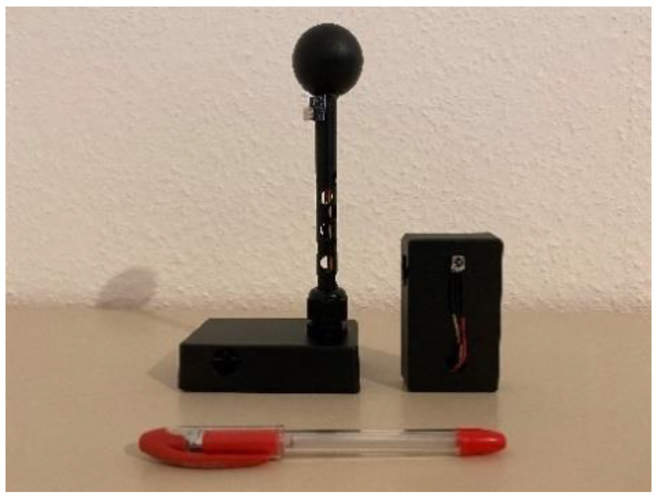
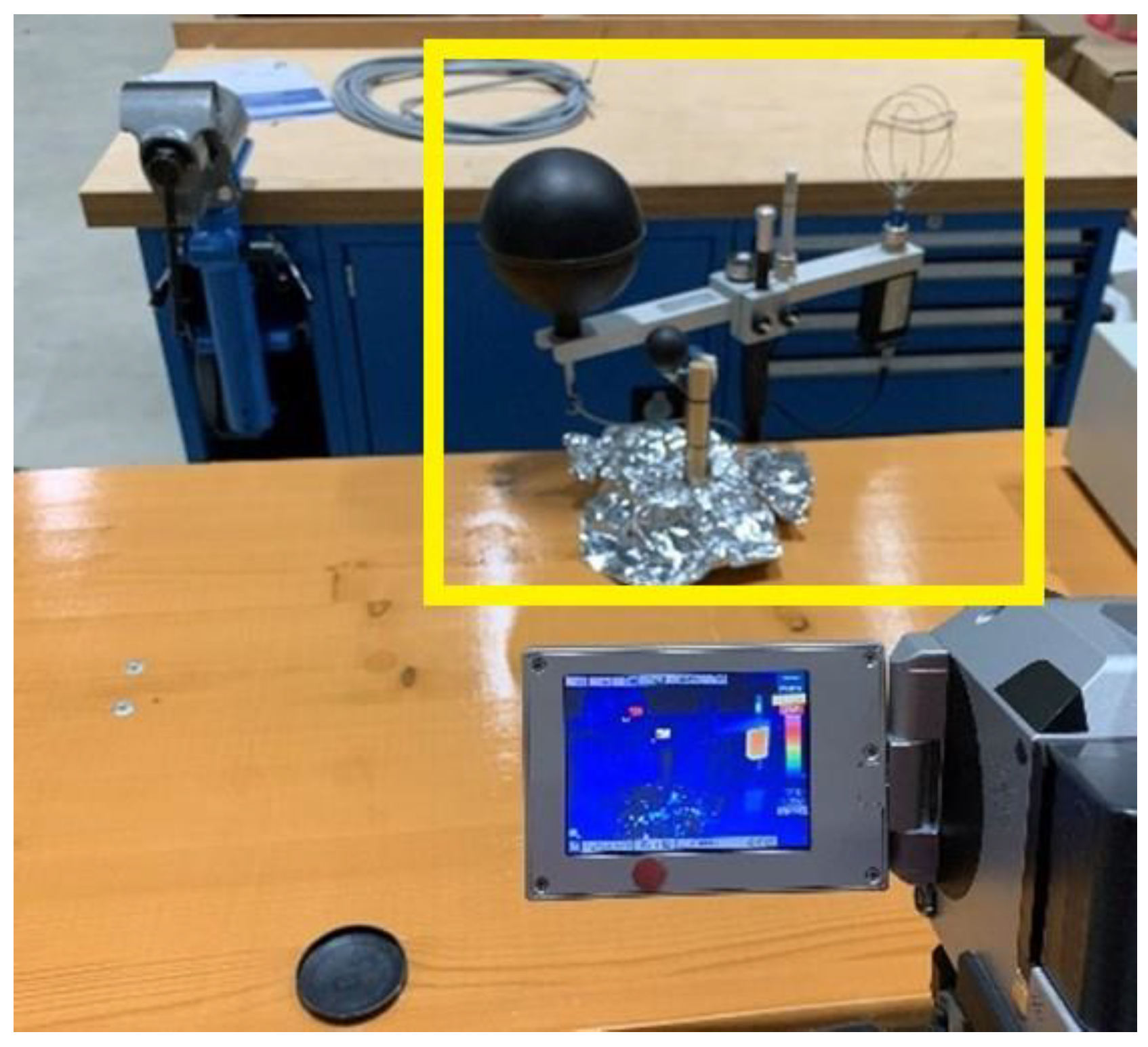
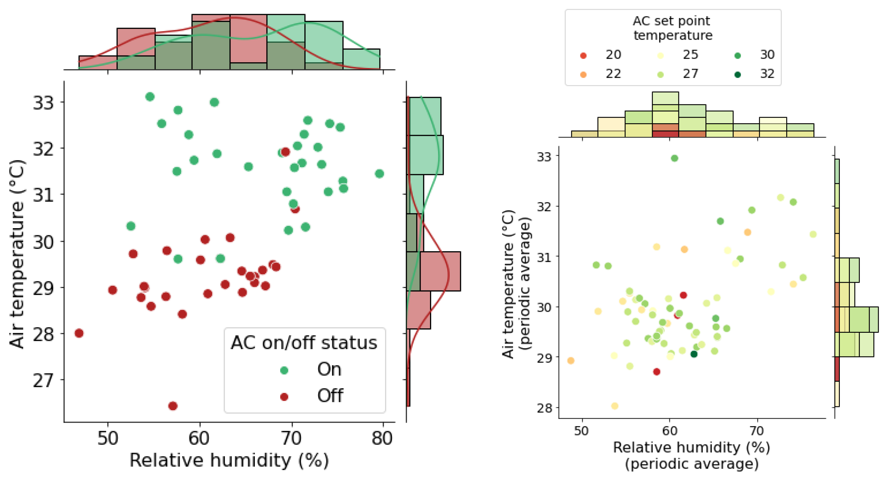
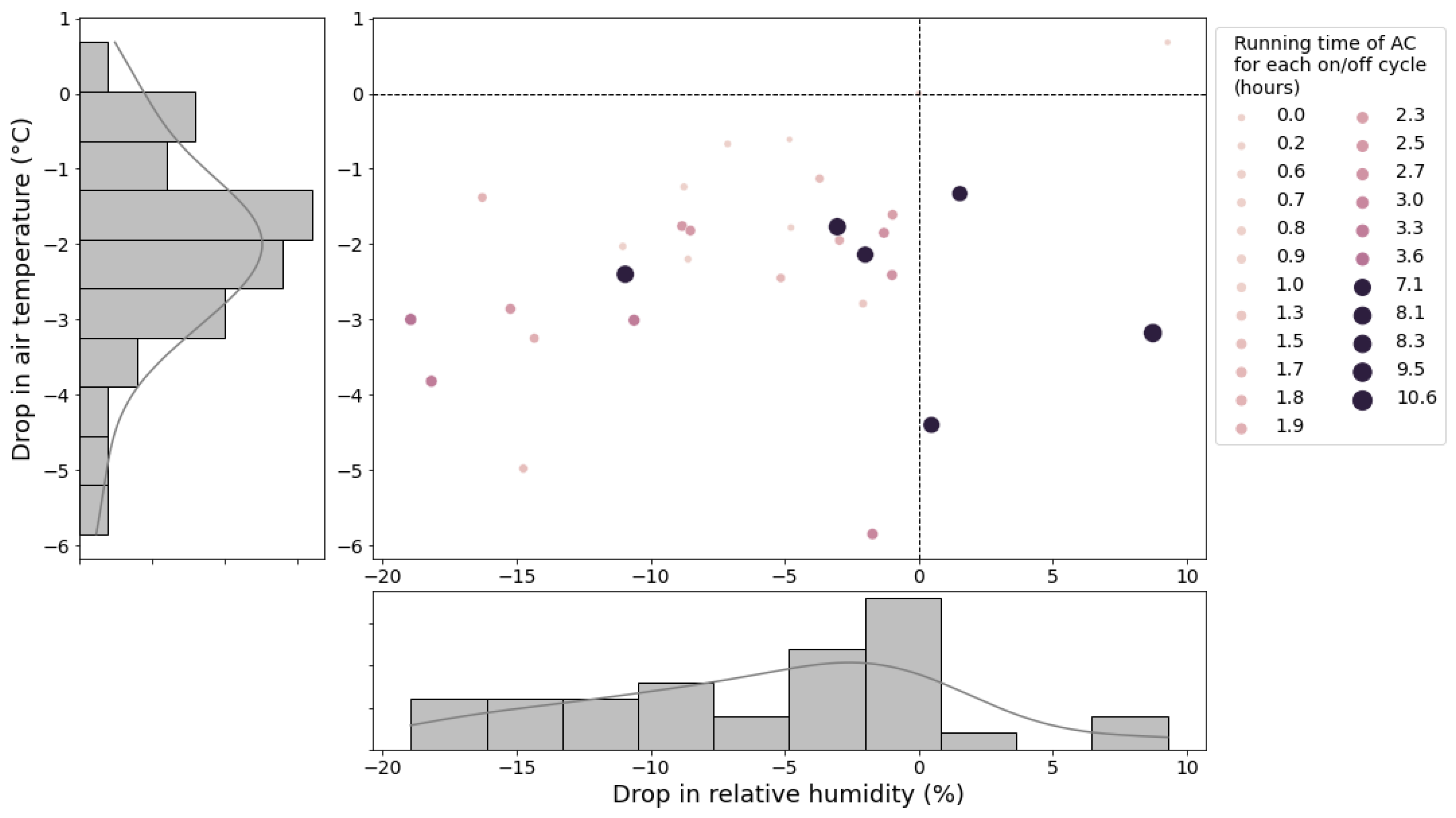
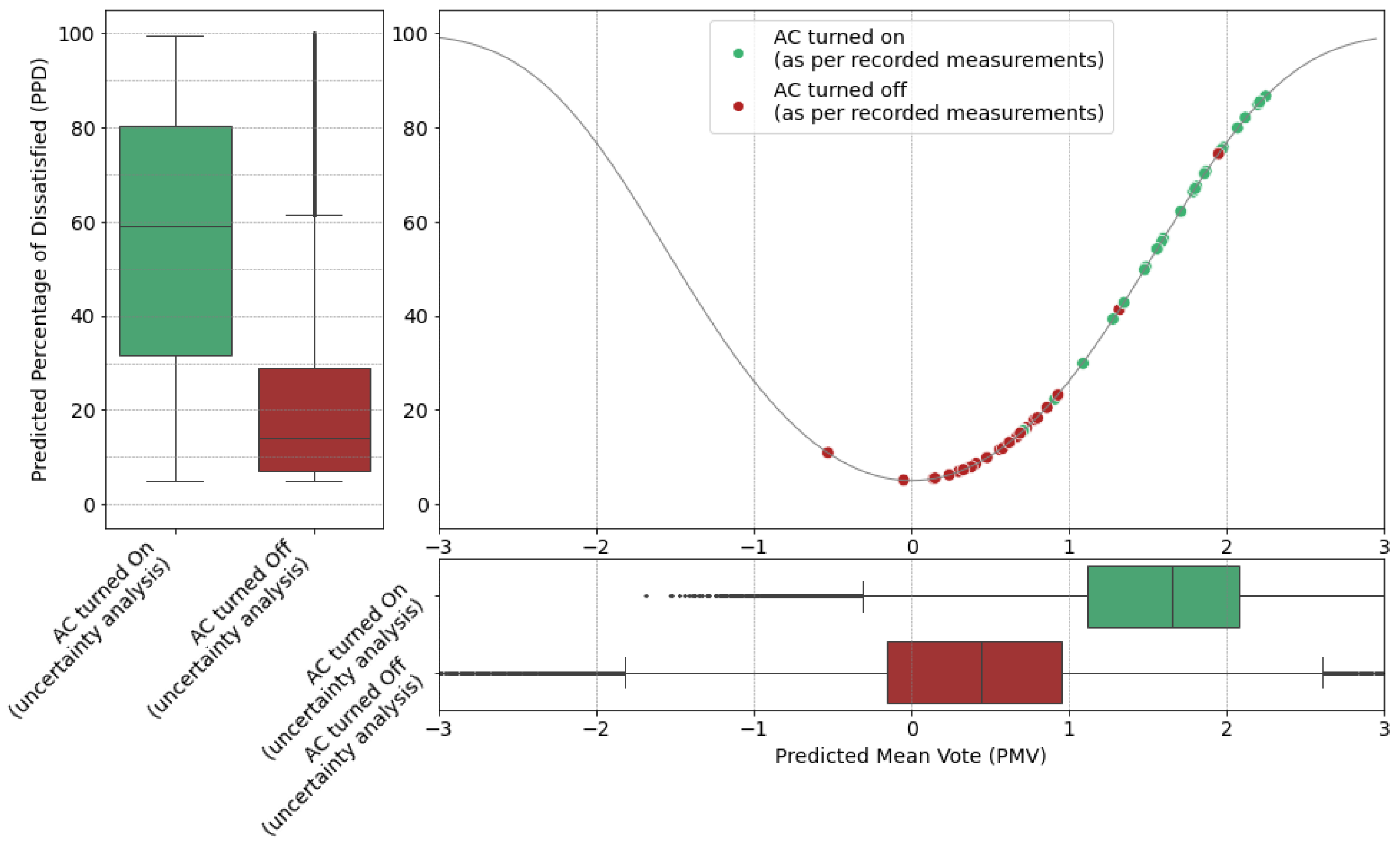
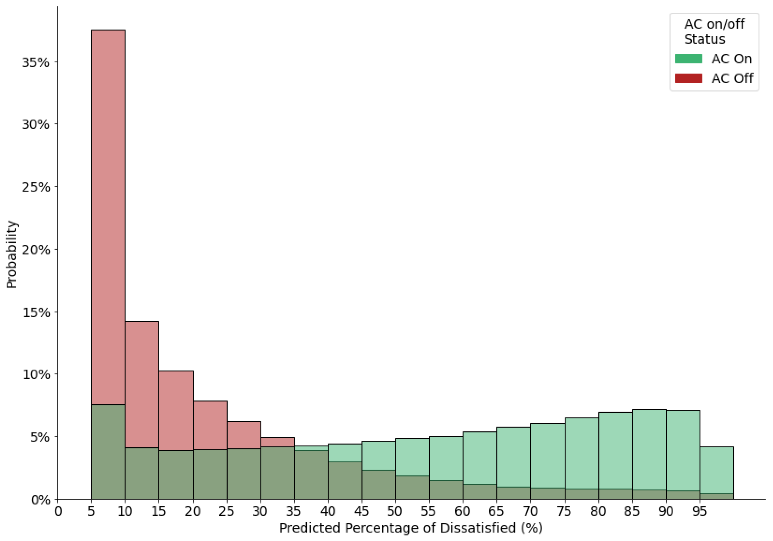
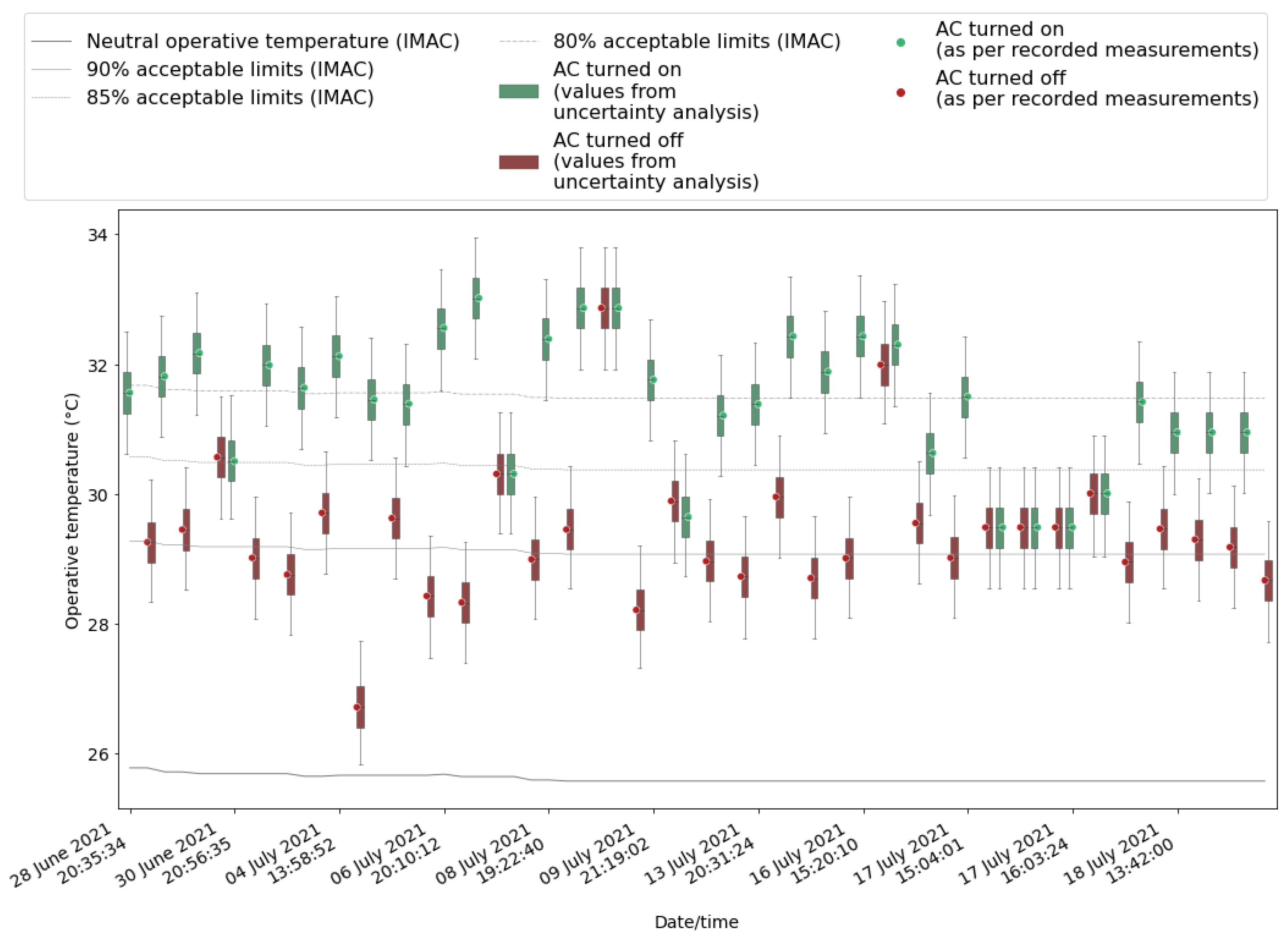
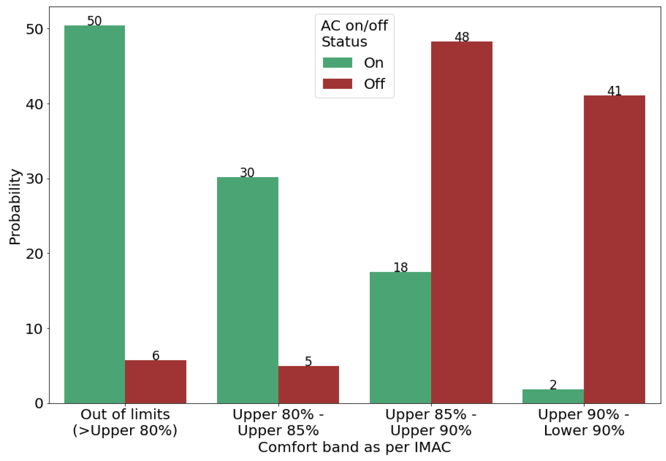
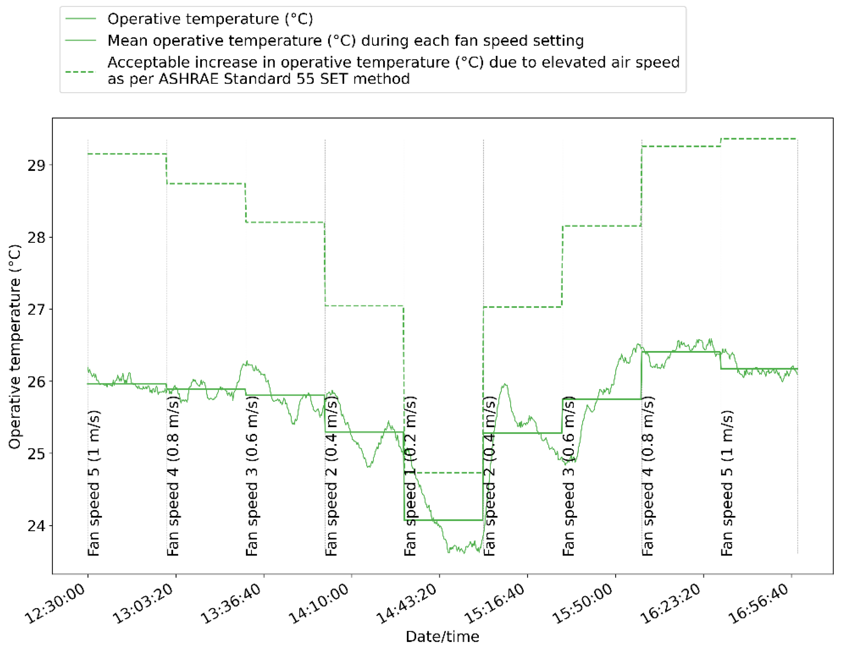
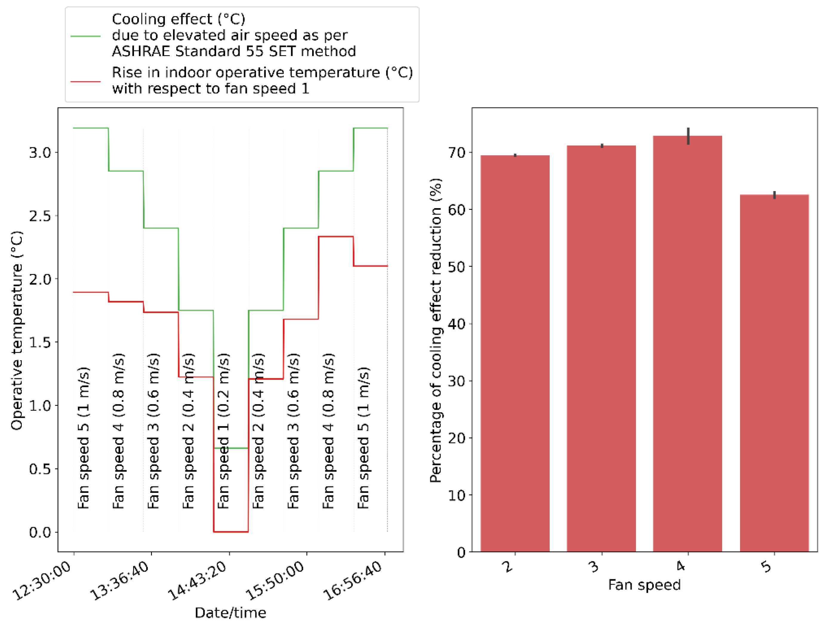
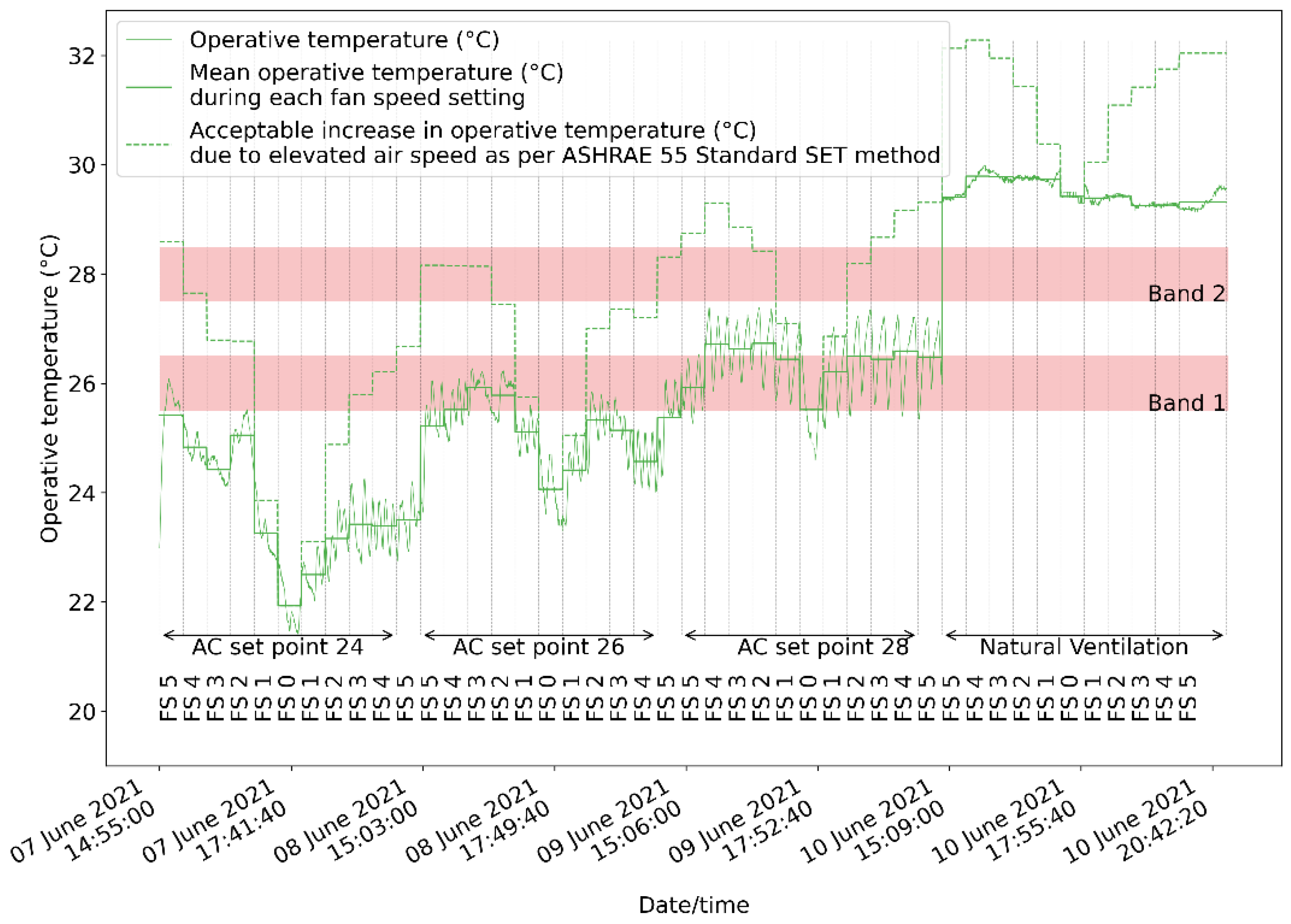
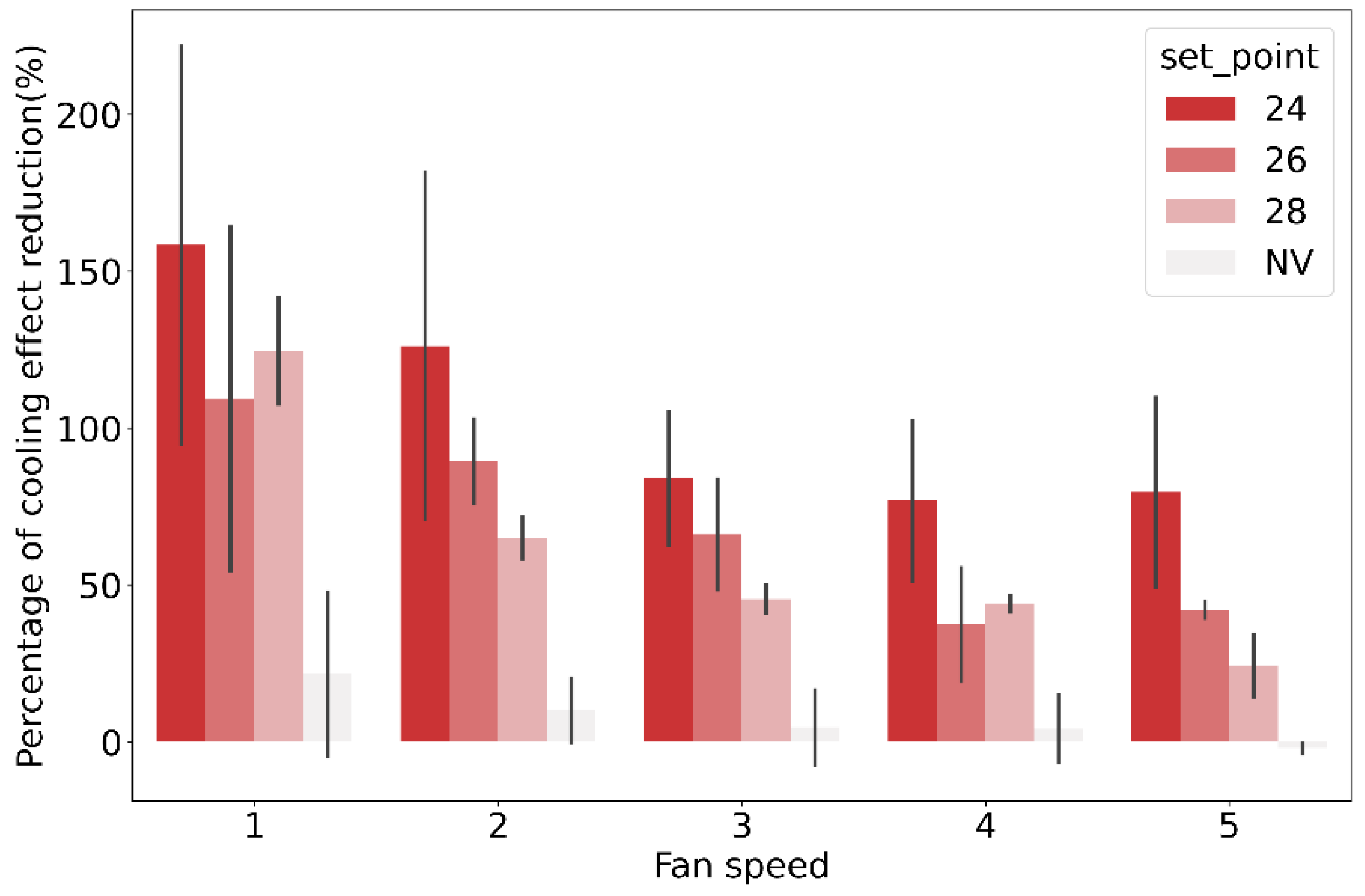
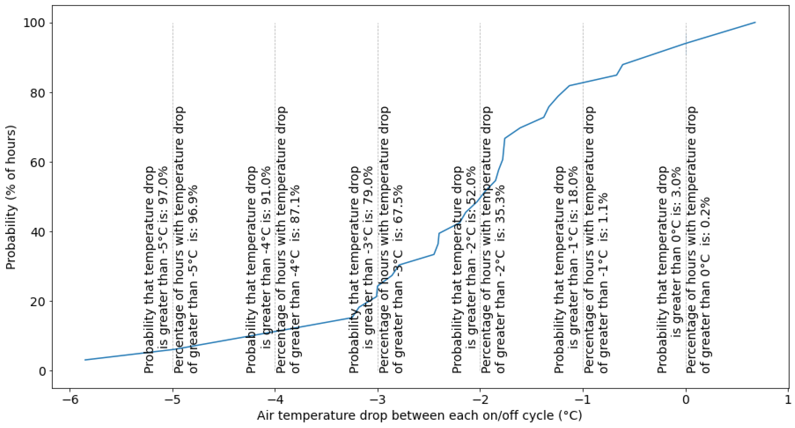
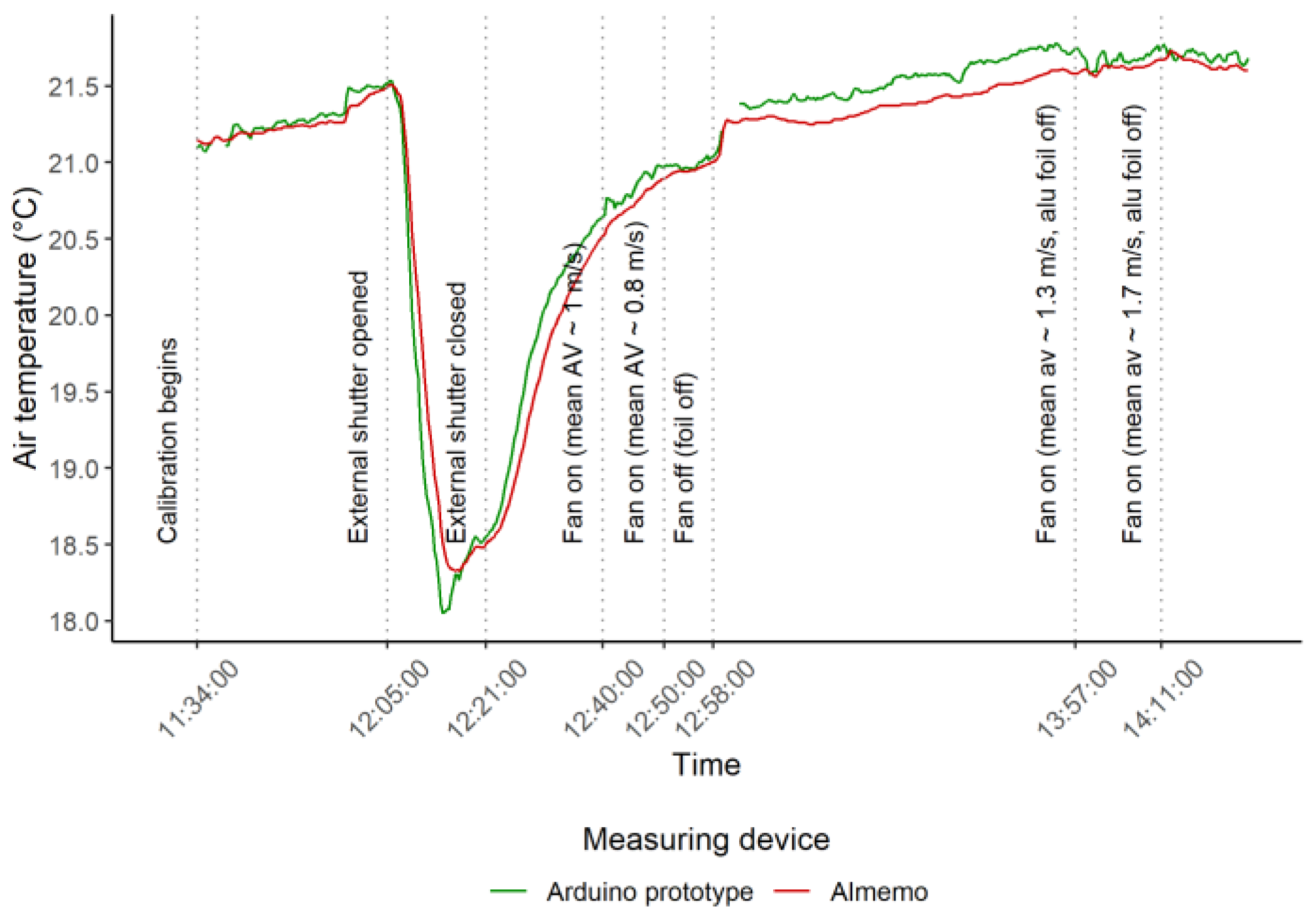
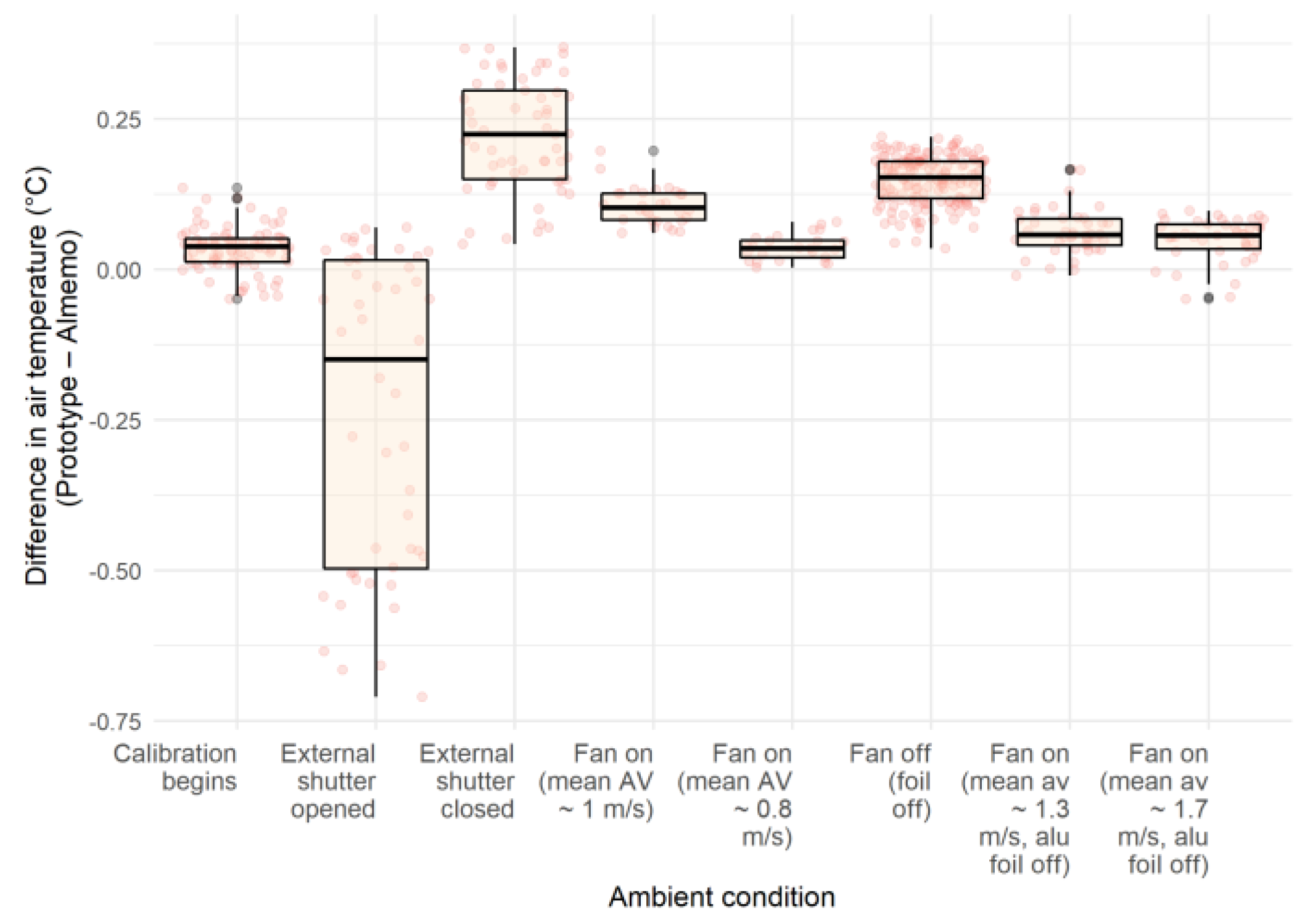
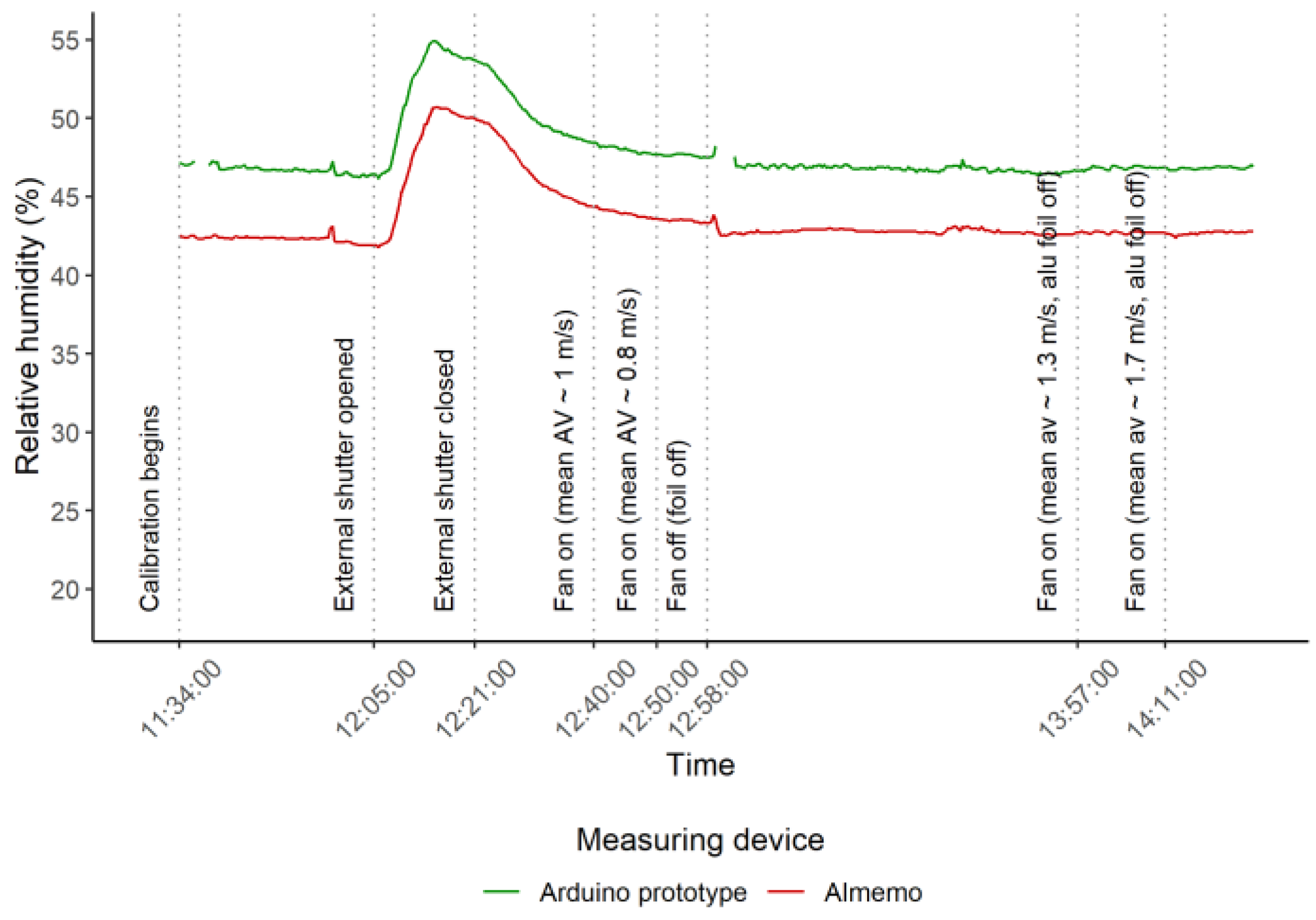
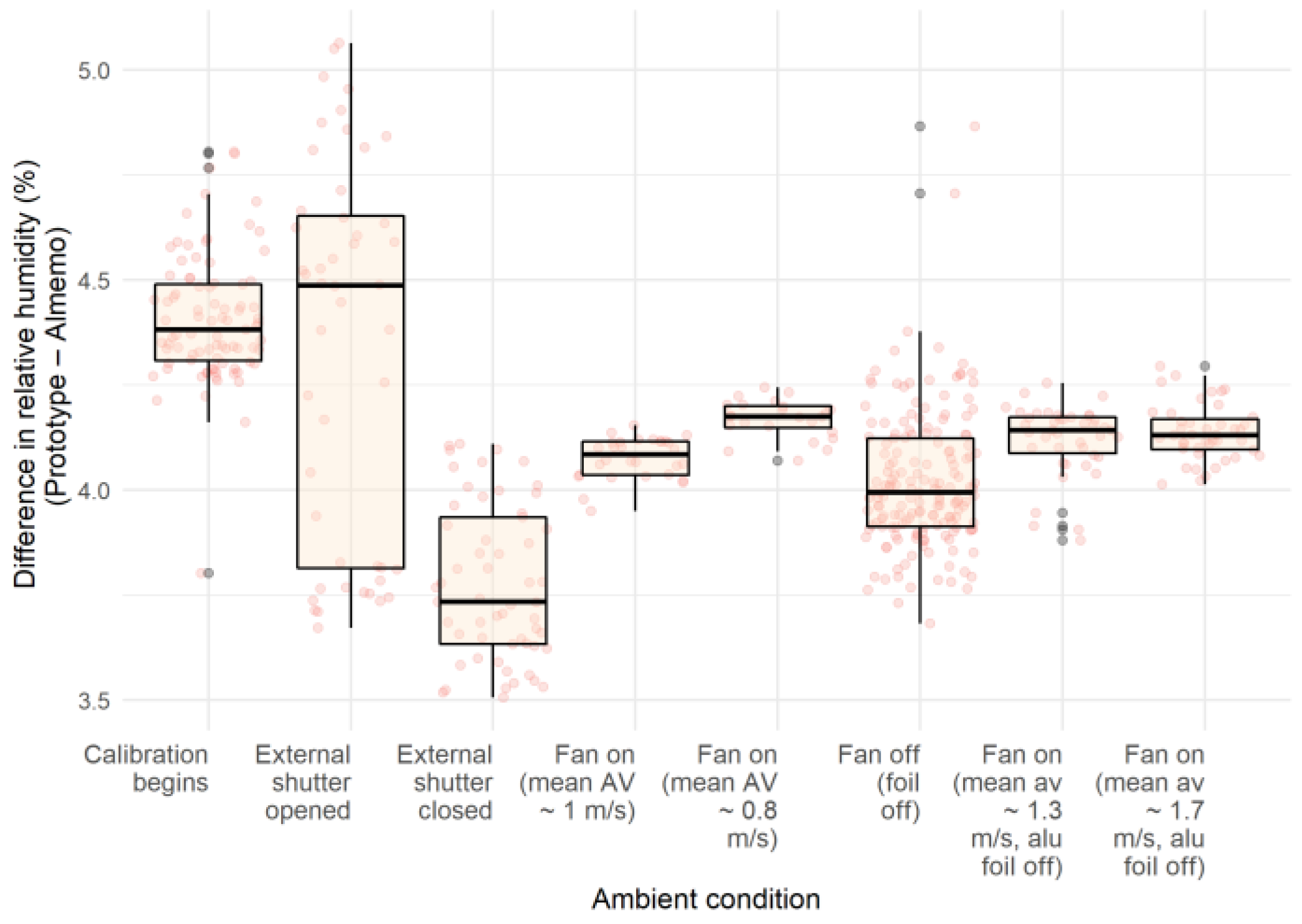
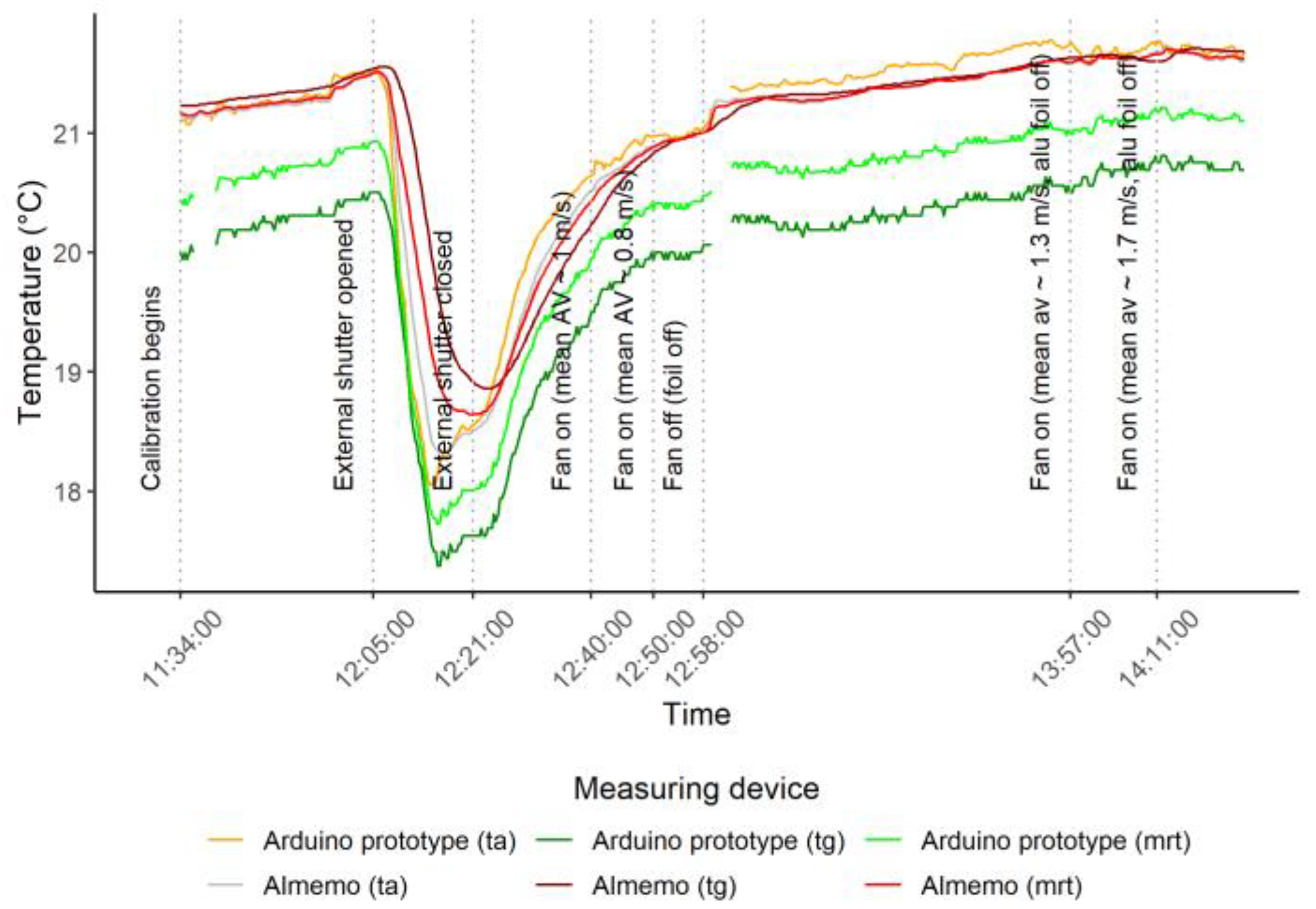
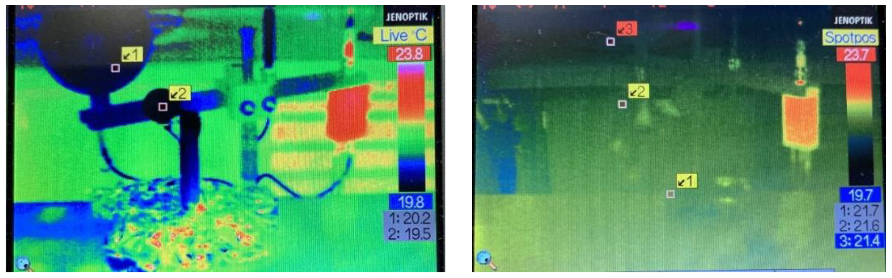
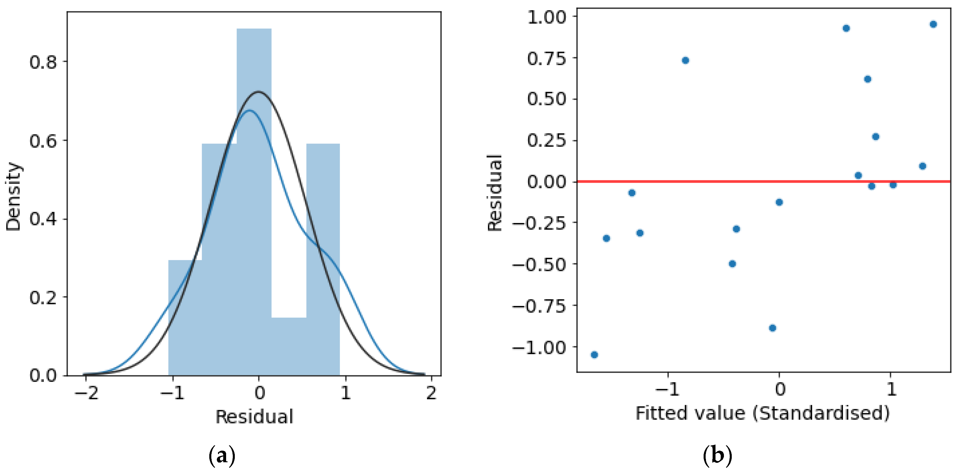